Applied Quantitative Analysis and Practices

LECTURE#11

By

Dr. Osman Sadiq Paracha

Previous Lecture Summary Scatter Plotting methods in SPSS Covariance Coefficient of Correlation Application in SPSS

Features of theCoefficient of Correlation

The population coefficient of correlation is referred as ρ. The sample coefficient of correlation is referred to as r. Either ρ or r have the following features:

Unit free Range between –1 and 1 The closer to –1, the stronger the negative linear relationship The closer to 1, the stronger the positive linear relationship The closer to 0, the weaker the linear relationship

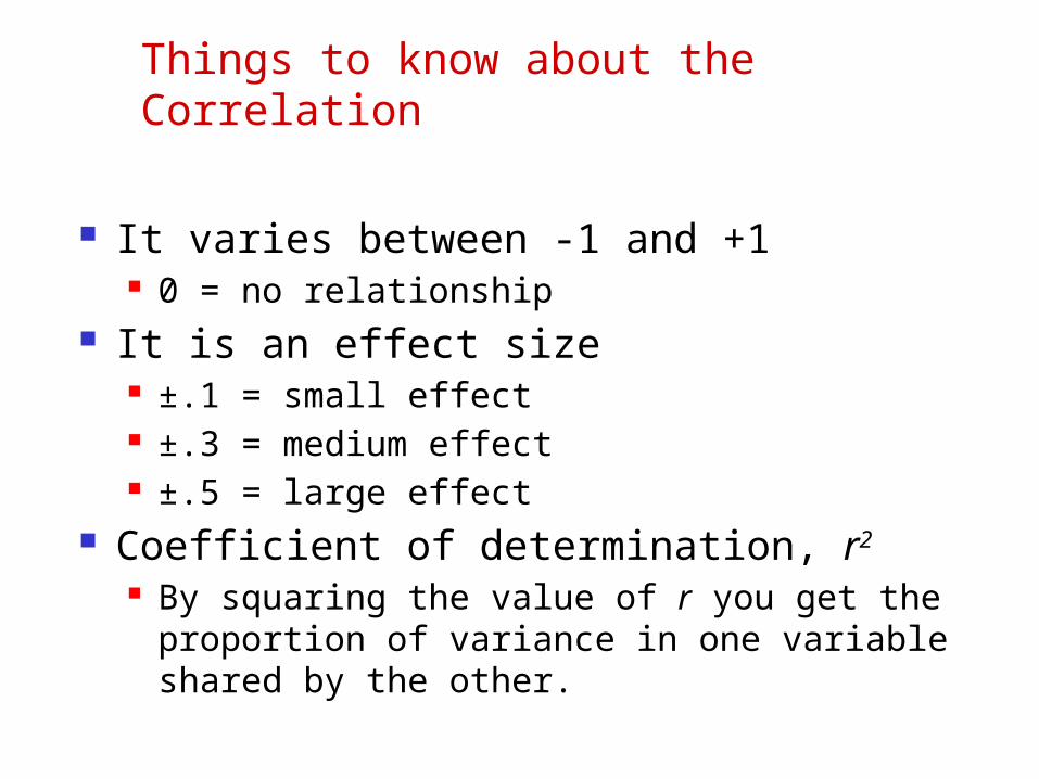
Things to know about the Correlation

It varies between -1 and +1 0 = no relationship

It is an effect size ±.1 = small effect ±.3 = medium effect ±.5 = large effect

Coefficient of determination, r2 By squaring the value of r you get the proportion of

variance in one variable shared by the other.

Correlation and Causality

The third-variable problem: in any correlation, causality between two variables

cannot be assumed because there may be other measured or unmeasured variables affecting the results.

Direction of causality: Correlation coefficients say nothing about which

variable causes the other to change

Correlation

Spearman’s Rho Pearson’s correlation on the ranked data

Kendall’s Tau Better than Spearman’s for small samples

Partial Correlations

Partial correlation: Measures the relationship between two variables,

controlling for the effect that a third variable has on them both

Scatter Plots of Sample Data with Various Coefficients of Correlation

Y

X

Y

X

Y

X

Y

X

r = -1 r = -.6

r = +.3r = +1

Y

Xr = 0

Pitfalls in Numerical Descriptive Measures

Data analysis is objective Should report the summary measures that best

describe and communicate the important aspects of the data set

Data interpretation is subjective Should be done in fair, neutral and clear manner

Ethical Considerations

Numerical descriptive measures:

Should document both good and bad results Should be presented in a fair, objective and

neutral manner Should not use inappropriate summary

measures to distort facts

The Normal Distribution

Discrete variables produce outcomes that come from a counting process (e.g. number of classes you are taking).

Continuous variables produce outcomes that come from a measurement (e.g. your annual salary, or your weight).

Types Of Variables

Types Of Variables

Discrete Variable

ContinuousVariable

Probability Distributions

Continuous Probability

Distributions

Binomial

Hypergeometric

Poisson

Probability Distributions

Discrete Probability

Distributions

Normal

Uniform

Exponential

Continuous Probability Distributions

A continuous random variable is a variable that can assume any value on a continuum (can assume an uncountable number of values) thickness of an item time required to complete a task temperature of a solution height, in inches

These can potentially take on any value depending only on the ability to precisely and accurately measure

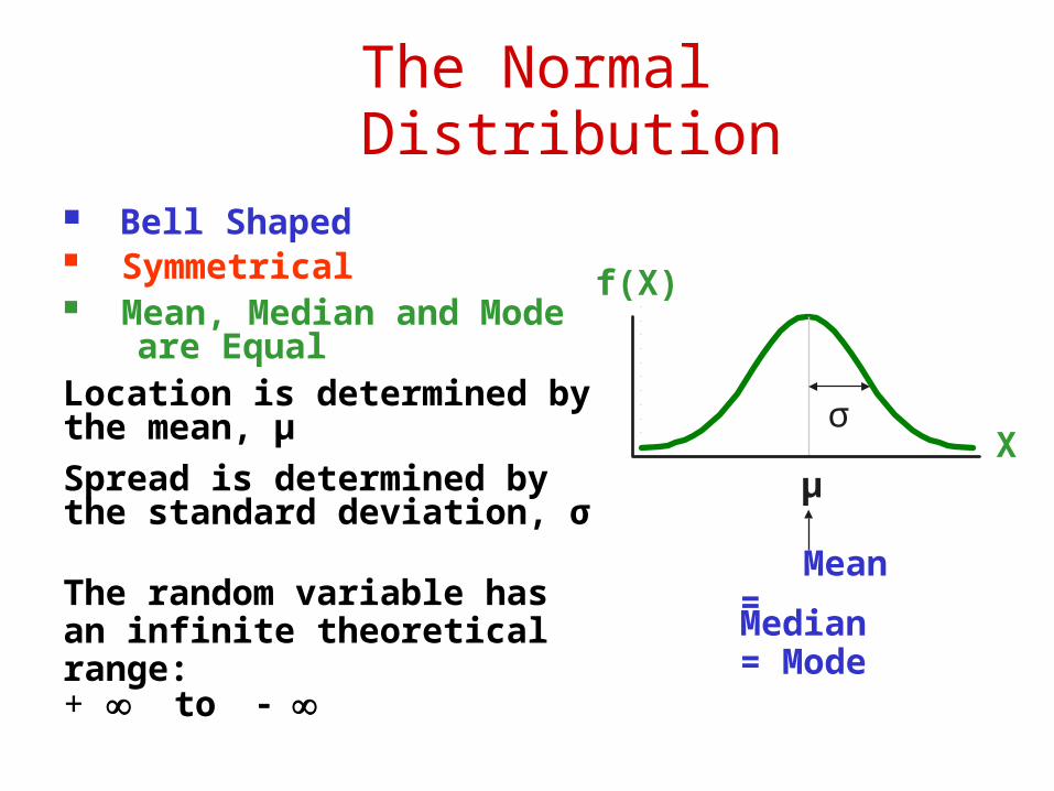
The Normal Distribution

‘Bell Shaped’ Symmetrical Mean, Median and Mode

are EqualLocation is determined by the mean, μ

Spread is determined by the standard deviation, σ

The random variable has an infinite theoretical range: + to

Mean = Median = Mode

X

f(X)

μ

σ

The Normal DistributionDensity Function

2μ)(X

2

1

e2π

1f(X)

The formula for the normal probability density function is

Where e = the mathematical constant approximated by 2.71828

π = the mathematical constant approximated by 3.14159

μ = the population mean

σ = the population standard deviation

X = any value of the continuous variable

By varying the parameters μ and σ, we obtain different normal distributions

ABC

A and B have the same mean but different standard deviations.

B and C have different means and different standard deviations.

The Normal Distribution Shape

X

f(X)

μ

σ

Changing μ shifts the distribution left or right.

Changing σ increases or decreases the spread.

The Standardized Normal

Any normal distribution (with any mean and standard deviation combination) can be transformed into the standardized normal distribution (Z)

To compute normal probabilities need to transform X units into Z units

The standardized normal distribution (Z) has a mean of 0 and a standard deviation of 1

Translation to the Standardized Normal Distribution

Translate from X to the standardized normal (the “Z” distribution) by subtracting the mean of X and dividing by its standard deviation:

σ

μXZ

The Z distribution always has mean = 0 and standard deviation = 1

The Standardized Normal Probability Density Function

The formula for the standardized normal probability density function is

Where e = the mathematical constant approximated by 2.71828

π = the mathematical constant approximated by 3.14159

Z = any value of the standardized normal distribution

2(1/2)Ze2π

1f(Z)

The Standardized Normal Distribution

Also known as the “Z” distribution Mean is 0 Standard Deviation is 1

Z

f(Z)

0

1

Values above the mean have positive Z-values. Values below the mean have negative Z-values.

Example

If X is distributed normally with mean of $100 and standard deviation of $50, the Z value for X = $200 is

This says that X = $200 is two standard deviations (2 increments of $50 units) above the mean of $100.

2.0$50

100$$200

σ

μXZ

Comparing X and Z units

Note that the shape of the distribution is the same, only the scale has changed. We can express the problem in the original units (X in dollars) or in standardized units (Z)

Z$100

2.00$200 $X(μ = $100, σ = $50)

(μ = 0, σ = 1)

Finding Normal Probabilities

a b X

f(X) P a X b( )≤

Probability is measured by the area under the curve

≤

P a X b( )<<=(Note that the probability of any individual value is zero)

f(X)

Xμ

Probability as Area Under the Curve

0.50.5

The total area under the curve is 1.0, and the curve is symmetric, so half is above the mean, half is below

1.0)XP(

0.5)XP(μ 0.5μ)XP(

The Standardized Normal Table

The Cumulative Standardized Normal table gives the probability less than a desired value of Z (i.e., from negative infinity to Z)

Z0 2.00

0.9772Example:

P(Z < 2.00) = 0.9772

The Standardized Normal Table

The value within the table gives the probability from Z = up to the desired Z value

.9772

2.0P(Z < 2.00) = 0.9772

The row shows the value of Z to the first decimal point

The column gives the value of Z to the second decimal point

2.0

.

.

.

(continued)

Z 0.00 0.01 0.02 …

0.0

0.1

General Procedure for Finding Normal Probabilities

Draw the normal curve for the problem in terms of X

Translate X-values to Z-values

Use the Standardized Normal Table

To find P(a < X < b) when X is distributed normally:

Finding Normal Probabilities Let X represent the time it takes (in seconds)

to download an image file from the internet. Suppose X is normal with a mean of18.0

seconds and a standard deviation of 5.0 seconds. Find P(X < 18.6)

18.6

X18.0

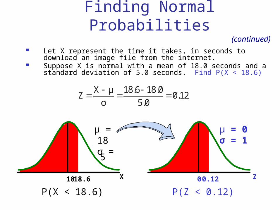
Let X represent the time it takes, in seconds to download an image file from the internet.

Suppose X is normal with a mean of 18.0 seconds and a standard deviation of 5.0 seconds. Find P(X < 18.6)

Z0.12 0X18.6 18

μ = 18 σ = 5

μ = 0σ = 1

(continued)

Finding Normal Probabilities

0.125.0

8.0118.6

σ

μXZ

P(X < 18.6) P(Z < 0.12)

Z

0.12

Z .00 .01

0.0 .5000 .5040 .5080

.5398 .5438

0.2 .5793 .5832 .5871

0.3 .6179 .6217 .6255

Solution: Finding P(Z < 0.12)

0.5478.02

0.1 .5478

Standardized Normal Probability Table (Portion)

0.00

= P(Z < 0.12)P(X < 18.6)

Finding NormalUpper Tail Probabilities

Suppose X is normal with mean 18.0 and standard deviation 5.0.

Now Find P(X > 18.6)

X

18.6

18.0

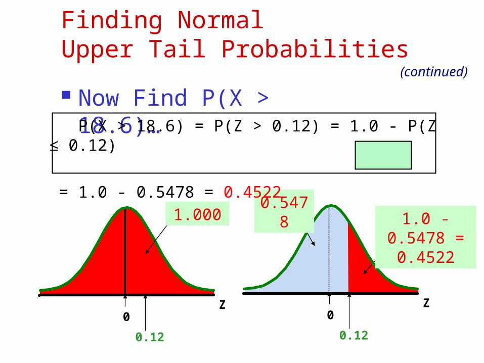
Now Find P(X > 18.6)…(continued)

Z

0.12

0Z

0.12

0.5478

0

1.000 1.0 - 0.5478 = 0.4522

P(X > 18.6) = P(Z > 0.12) = 1.0 - P(Z ≤ 0.12)

= 1.0 - 0.5478 = 0.4522

Finding NormalUpper Tail Probabilities

Lecture Summary Coefficient of Correlation in SPSS Application in SPSS Partial Correlation Ethical Considerations Normal Distribution