Embed Size (px)
Citation preview
Applied Math Algorithms in FACETS
Speaker: Lois Curfman McInnes, ANL Core: Alexander Pletzer, Tech-X
John Cary, Johan Carlsson, Tech-X: Core solver Srinath Vadlamani, Tech-X: Turbulent flux computation via FMCFM Ammar Hakim, Mahmood Miah, Tech-X: FACETS infrastructure Greg Hammett, PPPL: Time stepping schemes Alexei Pankin, Lehigh University: Core transport benchmark against ASTRA
Edge: Tom Rognlien, LLNL Satish Balay, ANL: Portability and systems issues via TOPS John Cary et al., Tech-X: FACETS integration Ron Cohen, LLNL: Edge physics, scripting Ben Dudson, Univ of York: BOUT++ physics and design, no FACETS funding Sean Farley, IIT: Math grad student: BOUT++ solvers and componentization Mike McCourt, Cornell: Applied math grad student: UEDGE solvers Maxim Umansky, LLNL: BOUT++ physics, no FACETS funding Hong Zhang, ANL: Nonlinear solvers
Coupling: Don Estep, CSU Brendan Sheehan, Simon Tavener, CSU: Stability and accuracy issues in coupling Ammar Hakim, Tech-X: Explicit coupling in FACETS Johan Carlsson, Tech-X: Implicit coupling in FACETS Ron Cohen, Tom Rognlien, LLNL: Physics issues in coupling
Proto-FSP Review, Sept 1, 2010, PPPL!
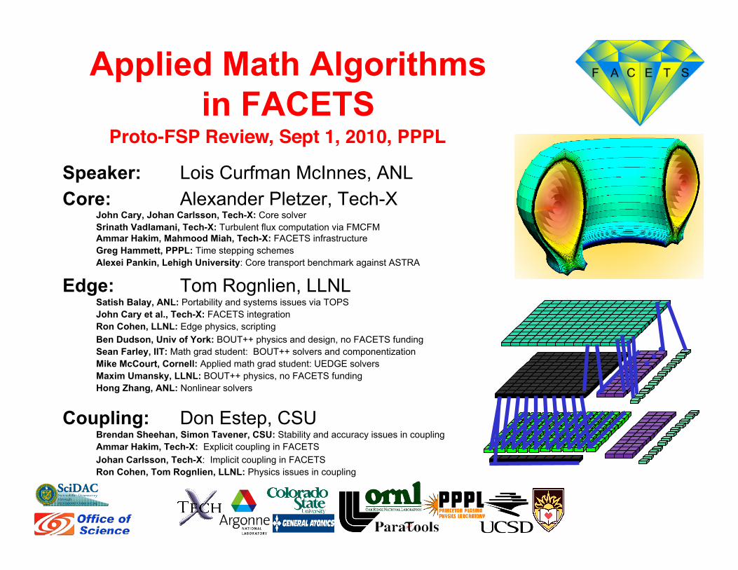
FACETS simulations rely on time-dependent, nonlinear PDEs
● Current focus Core (new core solver, Tech-X) Edge (UEDGE and BOUT++,
LLNL) Core-edge coupling
● Discussion emphasizes Collaboration with SciDAC
TOPS Center Implicit algorithms Scalability Stability and accuracy issues
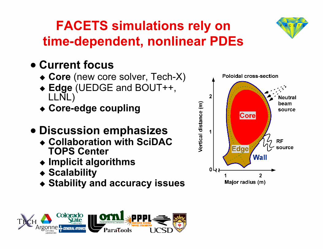
TOPS provides enabling technology to FACETS; FACETS motivates enhancements to TOPS
TOPS Overview • TOPS develops, demonstrates, and disseminates robust,
quality engineered, solver software for high-performance computers • TOPS institutions: ANL, LBNL, LLNL, SNL, Columbia U, Southern Methodist U, U of California, Berkeley, U of Colorado, Boulder, U of Texas, Austin
PI: D. Keyes, Columbia Univ.!www.scalablesolvers.org!
Towards Optimal Petascale Simulations!
Optimizer!
Linear solver!
Eigensolver!
Time integrator"
Nonlinear solver"
Indicates dependence"
Sensitivity Analyzer!SUNDIALS, Trilinos!TAO, Trilinos!
PARPACK, SuperLU, Trilinos!
hypre, PETSc, SuperLU, Trilinos!
PETSc, Trilinos!
PETSc, SUNDIALS, Trilinos!
Primary emphasis of TOPS numerical software!
FACETS fusion! CS!
Math!
Applications!
TOPS!
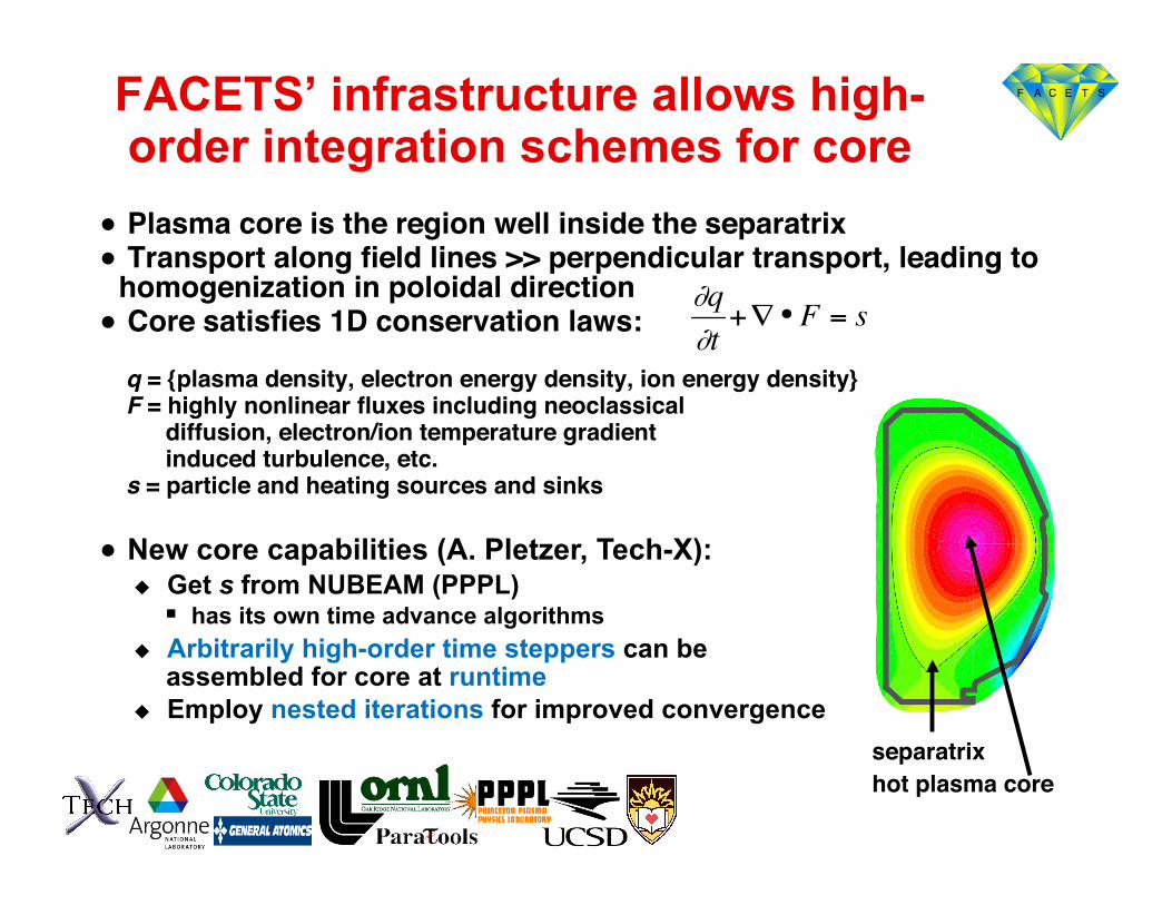
FACETS’ infrastructure allows high-order integration schemes for core
● Plasma core is the region well inside the separatrix!● Transport along field lines >> perpendicular transport, leading to
homogenization in poloidal direction!● Core satisfies 1D conservation laws:!
q = {plasma density, electron energy density, ion energy density} !F = highly nonlinear fluxes including neoclassical ! diffusion, electron/ion temperature gradient ! induced turbulence, etc.!s = particle and heating sources and sinks!
● New core capabilities (A. Pletzer, Tech-X): Get s from NUBEAM (PPPL)
has its own time advance algorithms Arbitrarily high-order time steppers can be
assembled for core at runtime Employ nested iterations for improved convergence
separatrix!hot plasma core!
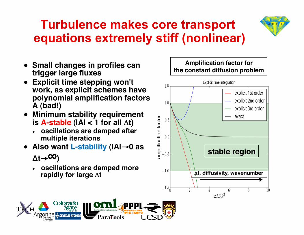
Turbulence makes core transport equations extremely stiff (nonlinear)
● Small changes in profiles can trigger large fluxes!
● Explicit time stepping won't work, as explicit schemes have polynomial amplification factors A (bad!)!
● Minimum stability requirement is A-stable (|A| < 1 for all Δt)!● oscillations are damped after
multiple iterations!● Also want L-stability (|A|→0 as Δt→∞)!● oscillations are damped more
rapidly for large Δt!
stable region!
Amplification factor for!the constant diffusion problem!
Δt, diffusivity, wavenumber !
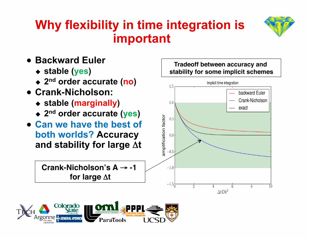
Why flexibility in time integration is important
● Backward Euler stable (yes) 2nd order accurate (no)
● Crank-Nicholson: stable (marginally) 2nd order accurate (yes)
● Can we have the best of both worlds? Accuracy and stability for large Δt
Crank-Nicholsonʼs A → -1 for large Δt!
Tradeoff between accuracy and stability for some implicit schemes!
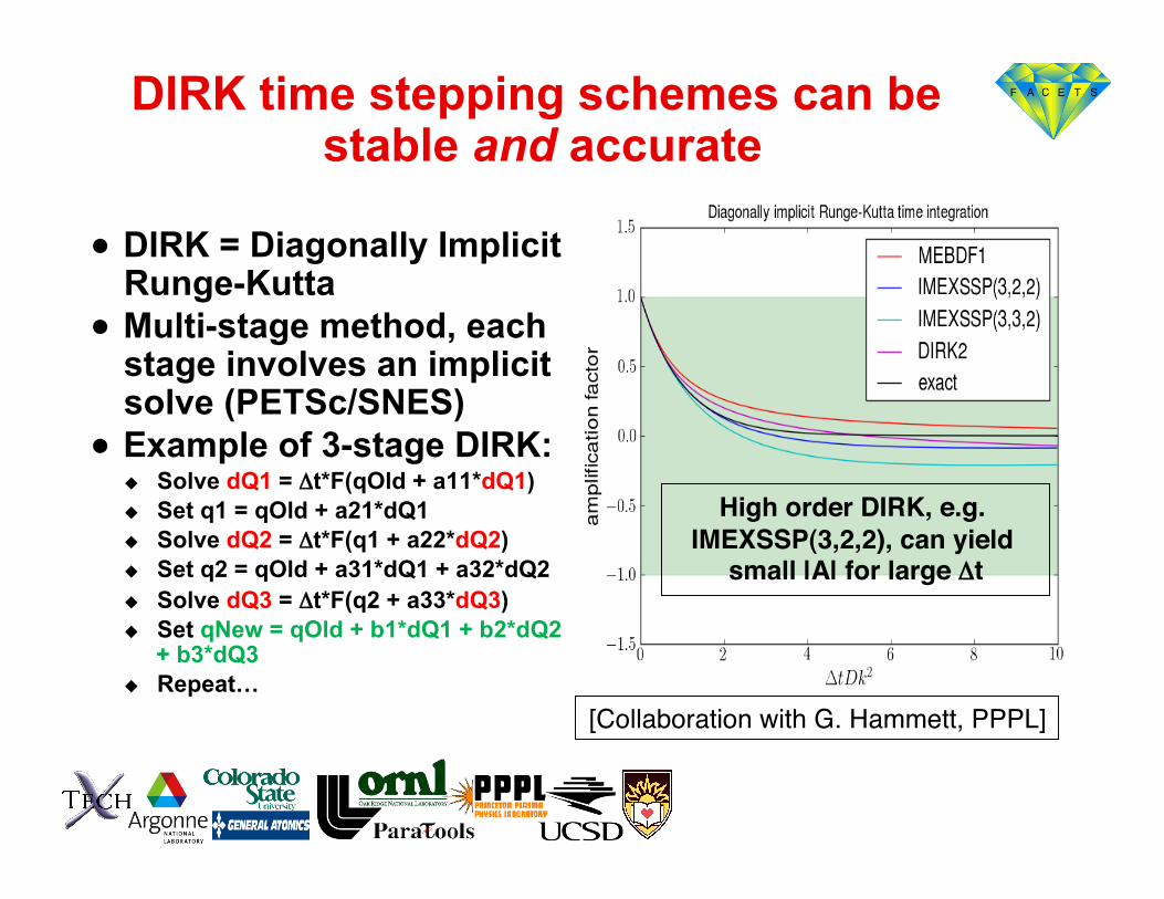
DIRK time stepping schemes can be stable and accurate
● DIRK = Diagonally Implicit Runge-Kutta
● Multi-stage method, each stage involves an implicit solve (PETSc/SNES)
● Example of 3-stage DIRK: Solve dQ1 = Δt*F(qOld + a11*dQ1) Set q1 = qOld + a21*dQ1 Solve dQ2 = Δt*F(q1 + a22*dQ2) Set q2 = qOld + a31*dQ1 + a32*dQ2 Solve dQ3 = Δt*F(q2 + a33*dQ3) Set qNew = qOld + b1*dQ1 + b2*dQ2
+ b3*dQ3 Repeat…
[Collaboration with G. Hammett, PPPL]"
High order DIRK, e.g. IMEXSSP(3,2,2), can yield
small |A| for large Δt!
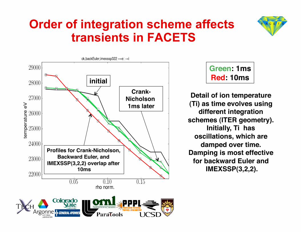
Order of integration scheme affects transients in FACETS
Detail of ion temperature (Ti) as time evolves using
different integration schemes (ITER geometry).
Initially, Ti has oscillations, which are
damped over time. Damping is most effective
for backward Euler and IMEXSSP(3,2,2).!
initial!Crank-
Nicholson 1ms later!
Profiles for Crank-Nicholson, Backward Euler, and
IMEXSSP(3,2,2) overlap after 10ms!
Green: 1ms!Red: 10ms!
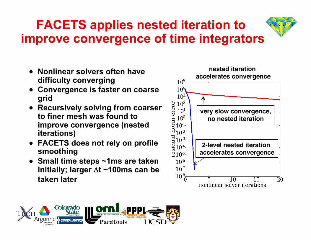
FACETS applies nested iteration to improve convergence of time integrators
● Nonlinear solvers often have difficulty converging
● Convergence is faster on coarse grid
● Recursively solving from coarser to finer mesh was found to improve convergence (nested iterations)
● FACETS does not rely on profile smoothing
● Small time steps ~1ms are taken initially; larger Δt ~100ms can be taken later
very slow convergence,!no nested iteration!
2-level nested iteration accelerates convergence!
nested iteration !accelerates convergence!
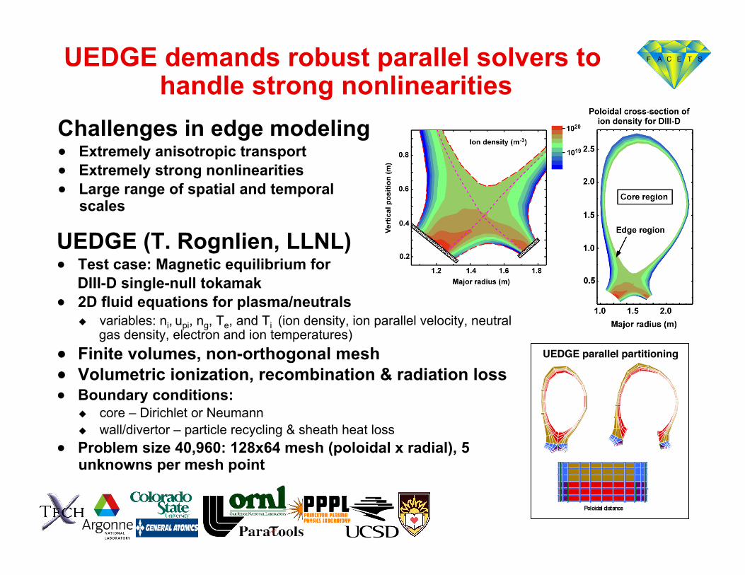
UEDGE (T. Rognlien, LLNL) ● Test case: Magnetic equilibrium for DIII-D single-null tokamak ● 2D fluid equations for plasma/neutrals
variables: ni, upi, ng, Te, and Ti (ion density, ion parallel velocity, neutral gas density, electron and ion temperatures)
● Finite volumes, non-orthogonal mesh ● Volumetric ionization, recombination & radiation loss ● Boundary conditions:
core – Dirichlet or Neumann wall/divertor – particle recycling & sheath heat loss
● Problem size 40,960: 128x64 mesh (poloidal x radial), 5 unknowns per mesh point
UEDGE demands robust parallel solvers to handle strong nonlinearities
Challenges in edge modeling ● Extremely anisotropic transport ● Extremely strong nonlinearities ● Large range of spatial and temporal
scales
UEDGE parallel partitioning!
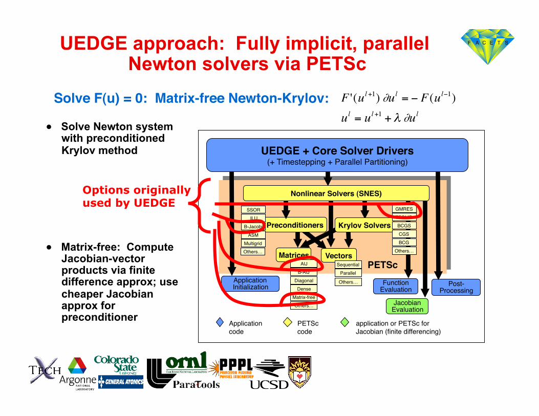
UEDGE approach: Fully implicit, parallel Newton solvers via PETSc
Solve F(u) = 0: Matrix-free Newton-Krylov:!● Solve Newton system
with preconditioned Krylov method
● Matrix-free: Compute Jacobian-vector products via finite difference approx; use cheaper Jacobian approx for preconditioner
Post-"Processing"
Application"Initialization" Function"
Evaluation"
Jacobian"Evaluation"
PETSc!
PETSc "code"
Application code"
application or PETSc for "Jacobian (finite differencing)"
Matrices! Vectors!
Krylov Solvers!Preconditioners!
GMRES"TFQMR"BCGS"CGS"BCG"
Others…"
SSOR"ILU"
B-Jacobi"ASM"
Multigrid"Others…"
AIJ"B-AIJ"
Diagonal"Dense"
Matrix-free"Others…"
Sequential"Parallel"
Others…"
UEDGE + Core Solver Drivers !(+ Timestepping + Parallel Partitioning)"
Nonlinear Solvers (SNES)!Options originally used by UEDGE
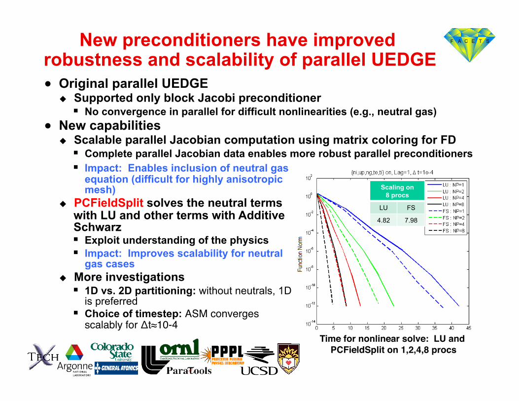
New preconditioners have improved robustness and scalability of parallel UEDGE ● Original parallel UEDGE
Supported only block Jacobi preconditioner No convergence in parallel for difficult nonlinearities (e.g., neutral gas)
● New capabilities Scalable parallel Jacobian computation using matrix coloring for FD
Complete parallel Jacobian data enables more robust parallel preconditioners Impact: Enables inclusion of neutral gas
equation (difficult for highly anisotropic mesh)
PCFieldSplit solves the neutral terms with LU and other terms with Additive Schwarz Exploit understanding of the physics Impact: Improves scalability for neutral
gas cases More investigations
1D vs. 2D partitioning: without neutrals, 1D is preferred
Choice of timestep: ASM converges scalably for Δt≈10-4!
Time for nonlinear solve: LU and PCFieldSplit on 1,2,4,8 procs!
Scaling on 8 procs
LU FS
4.82 7.98
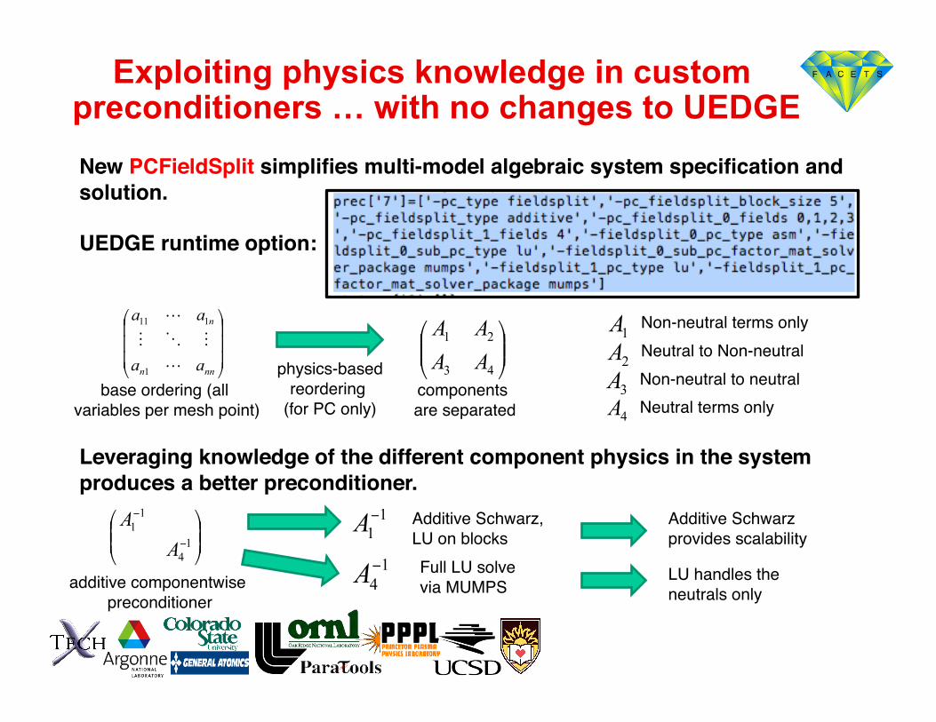
Exploiting physics knowledge in custom preconditioners … with no changes to UEDGE
Leveraging knowledge of the different component physics in the system produces a better preconditioner.!
additive componentwise preconditioner"
Additive Schwarz,"LU on blocks"Full LU solve via MUMPS"
Additive Schwarz provides scalability"
LU handles the neutrals only"
New PCFieldSplit simplifies multi-model algebraic system specification and solution. !
UEDGE runtime option:!
base ordering (all variables per mesh point)"
physics-based"reordering "
(for PC only)"components are separated"
Non-neutral to neutral "Neutral terms only"
Non-neutral terms only"Neutral to Non-neutral "
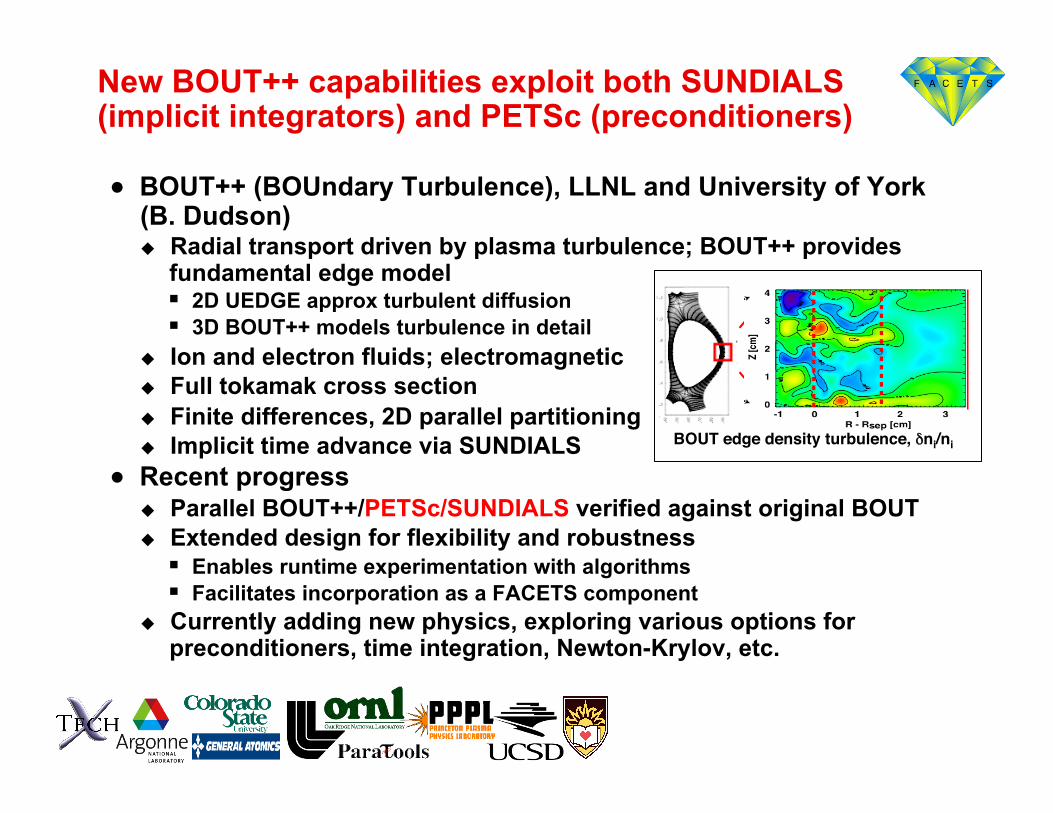
New BOUT++ capabilities exploit both SUNDIALS (implicit integrators) and PETSc (preconditioners)
● BOUT++ (BOUndary Turbulence), LLNL and University of York (B. Dudson) Radial transport driven by plasma turbulence; BOUT++ provides
fundamental edge model 2D UEDGE approx turbulent diffusion 3D BOUT++ models turbulence in detail
Ion and electron fluids; electromagnetic Full tokamak cross section Finite differences, 2D parallel partitioning Implicit time advance via SUNDIALS
● Recent progress Parallel BOUT++/PETSc/SUNDIALS verified against original BOUT Extended design for flexibility and robustness
Enables runtime experimentation with algorithms Facilitates incorporation as a FACETS component
Currently adding new physics, exploring various options for preconditioners, time integration, Newton-Krylov, etc.
BOUT edge density turbulence, δni/ni!
Several issues need to be resolved in a proper core-edge coupling scheme
● Initial conditions need to be consistent across the core edge boundary How to ensure two different models use the same initial
conditions? ● Flux models need to be consistent in both the core
and the edge at the core-edge interface How to ensure fluxes transition smoothly at the coupling
interface? ● Grids need to be carefully aligned to get second-
order coupling scheme How to ensure that spatial order is not reduced while
exchanging data across different grids? ● Temporal and spatial discretization need to be of the
same order for both models to maintain overall order
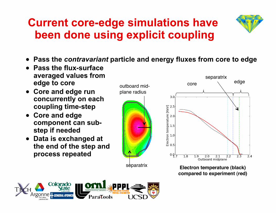
Current core-edge simulations have been done using explicit coupling
● Pass the contravariant particle and energy fluxes from core to edge
Electron temperature (black) compared to experiment (red) !
core" edge"outboard mid-plane radius"
separatrix"
separatrix"● Pass the flux-surface
averaged values from edge to core
● Core and edge run concurrently on each coupling time-step
● Core and edge component can sub-step if needed
● Data is exchanged at the end of the step and process repeated
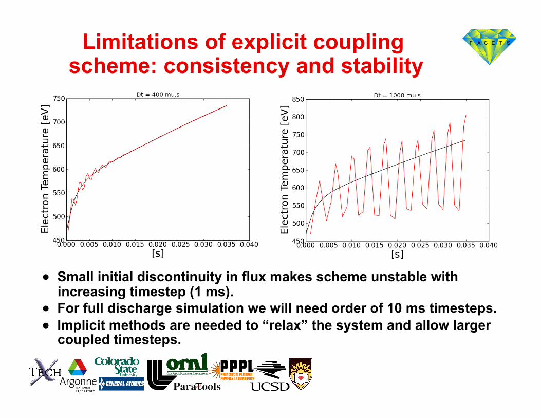
Limitations of explicit coupling scheme: consistency and stability
● Small initial discontinuity in flux makes scheme unstable with increasing timestep (1 ms).
● For full discharge simulation we will need order of 10 ms timesteps. ● Implicit methods are needed to “relax” the system and allow larger
coupled timesteps.
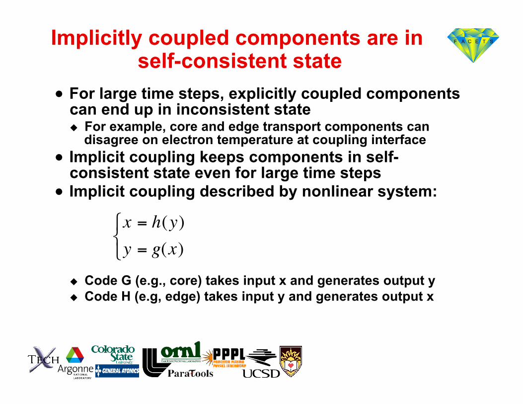
Implicitly coupled components are in self-consistent state
● For large time steps, explicitly coupled components can end up in inconsistent state For example, core and edge transport components can
disagree on electron temperature at coupling interface ● Implicit coupling keeps components in self-
consistent state even for large time steps ● Implicit coupling described by nonlinear system:
Code G (e.g., core) takes input x and generates output y Code H (e.g, edge) takes input y and generates output x
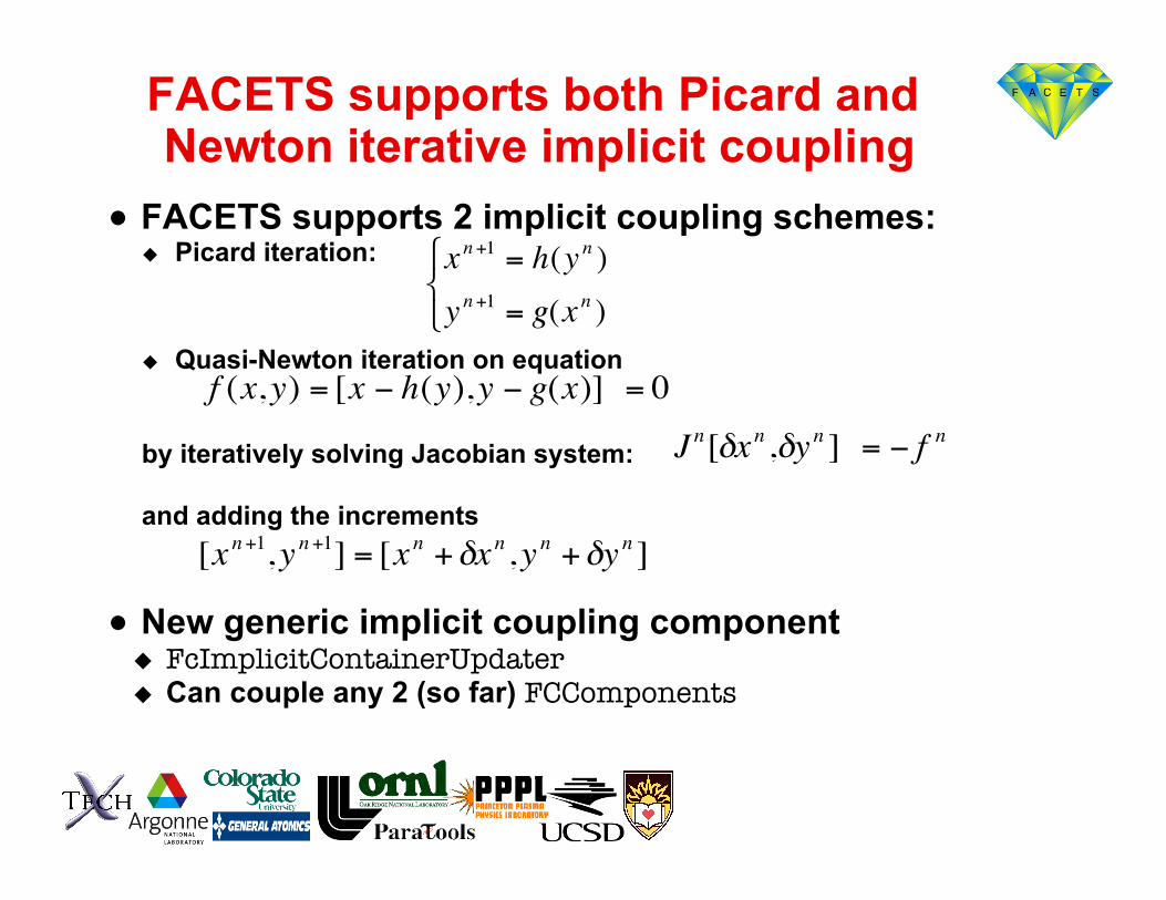
FACETS supports both Picard and Newton iterative implicit coupling
● FACETS supports 2 implicit coupling schemes: Picard iteration:
Quasi-Newton iteration on equation
by iteratively solving Jacobian system:
and adding the increments
● New generic implicit coupling component FcImplicitContainerUpdater Can couple any 2 (so far) FCComponents
€
f (x,y) = [x − h(y),y − g(x)] = 0
€
Jn[δxn ,δyn ] = − f n
€
[xn+1,yn+1] = [xn +δxn,yn +δyn ]
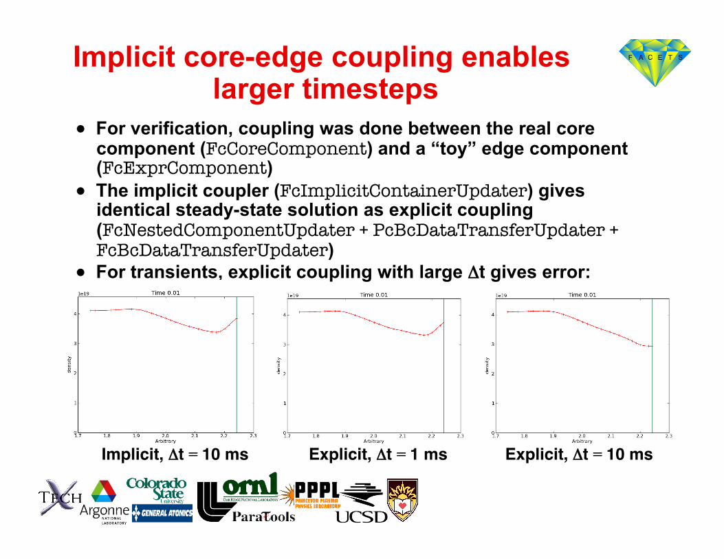
Implicit core-edge coupling enables larger timesteps
● For verification, coupling was done between the real core component (FcCoreComponent) and a “toy” edge component (FcExprComponent)
● The implicit coupler (FcImplicitContainerUpdater) gives identical steady-state solution as explicit coupling (FcNestedComponentUpdater + PcBcDataTransferUpdater + FcBcDataTransferUpdater)
● For transients, explicit coupling with large Δt gives error:
Implicit, Δt = 10 ms ! Explicit, Δt = 10 ms !Explicit, Δt = 1 ms !
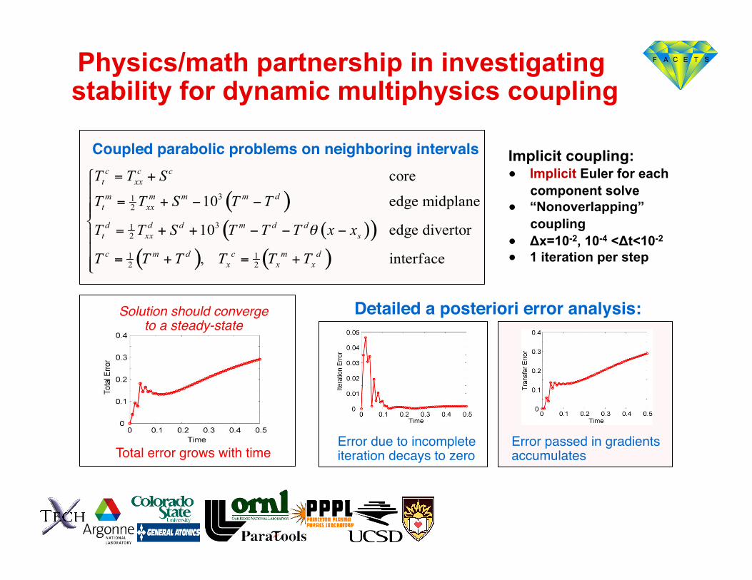
Physics/math partnership in investigating stability for dynamic multiphysics coupling
Implicit coupling: ● Implicit Euler for each
component solve ● “Nonoverlapping”
coupling ● Δx=10-2, 10-4 <Δt<10-2
● 1 iteration per step
Coupled parabolic problems on neighboring intervals!
Solution should converge!to a steady-state!
Total error grows with time"
Detailed a posteriori error analysis:!
Error due to incomplete iteration decays to zero"
Error passed in gradients accumulates"
Progress in analysis of accuracy and stability for multiphysics coupling
● A posteriori error analysis: Computational approach to error estimation that uses: Residuals to describe introduction of error Adjoint (dual) problems to describe the effect of stability Variational analysis to produce accurate error estimates The estimate provides a detailed description of causes of error This is a computational approach that can deal with complex problems
● Recent extensions multiscale, multiphysics models Treats general coupling strategies Handles differences in discretization scale and solution representation Handles complex stability of multiphysics problems
● Results (see http://www.math.colostate.edu/~estep )
● New CSU postdoc (B. Sheehan): Analyzing stability and error of core-edge coupling via hands-on work with physicists & FACETS framework
Coupling of elliptic/parabolic problems through a boundary (3 papers, 1 preprint)
Coupling of elliptic problems through parameter passing (1 paper, 1 preprint)
Overview book chapter
Operator splitting and multirate integration methods (1 paper, 2 preprints)
Extension to finite volume schemes (1 paper, 1 preprint)
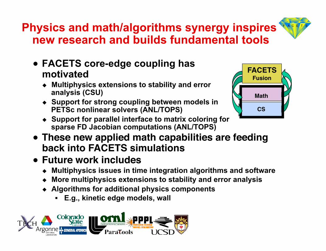
Physics and math/algorithms synergy inspires new research and builds fundamental tools
● FACETS core-edge coupling has motivated Multiphysics extensions to stability and error
analysis (CSU) Support for strong coupling between models in
PETSc nonlinear solvers (ANL/TOPS) Support for parallel interface to matrix coloring for
sparse FD Jacobian computations (ANL/TOPS) ● These new applied math capabilities are feeding
back into FACETS simulations!● Future work includes!
Multiphysics issues in time integration algorithms and software More multiphysics extensions to stability and error analysis Algorithms for additional physics components
E.g., kinetic edge models, wall
CS!
Math!
FACETS!Fusion!