Slide 1

Applied Geophysics –

Nov 8 -

10

EM induction methods

Amperes Law

Faradays Law

Basics of EM induction

Use EM31 as a specific learning example

Tx Rx

EOSC 350 ‘06 Slide 2

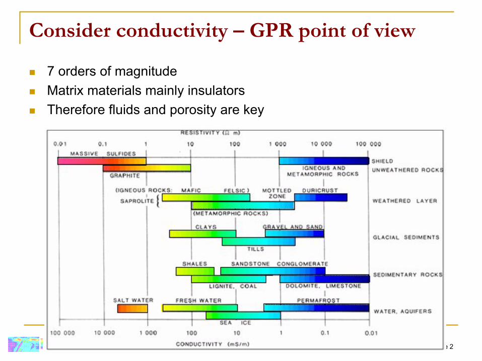
Consider conductivity –

GPR point of view

7 orders of magnitude

Matrix materials mainly insulators

Therefore fluids and porosity are key

EOSC 350 ‘06 Slide 3

HO

M

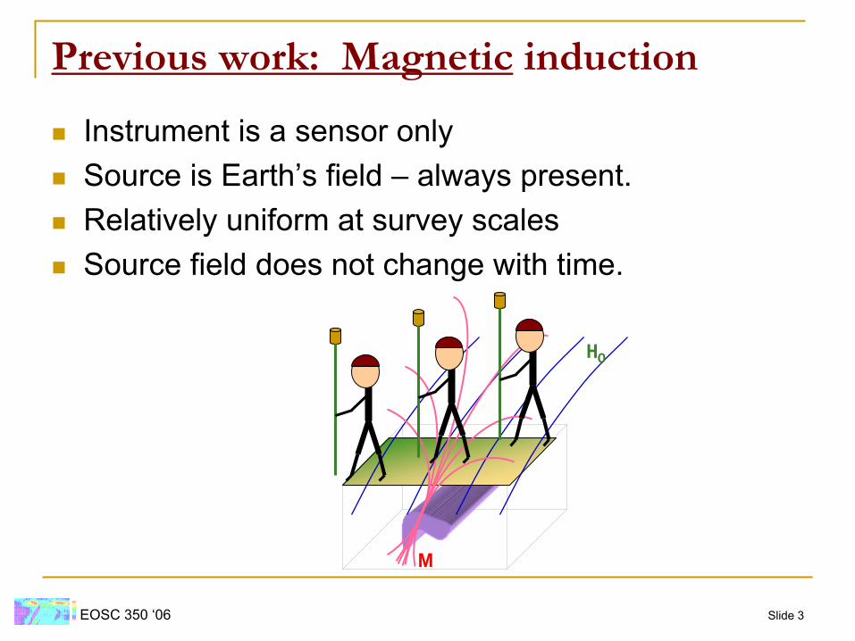
Previous work: Magnetic

induction

Instrument is a sensor only

Source is Earth’s field –

always present.

Relatively uniform at survey scales

Source field does not change with time.

EOSC 350 ‘06 Slide 4

Tx Rx

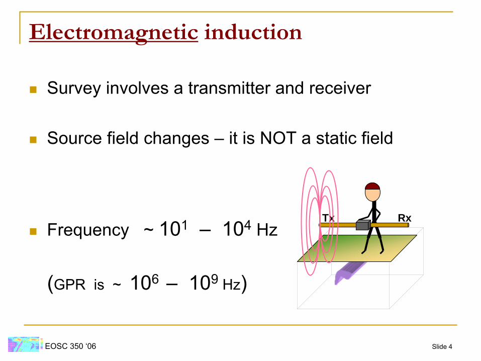
Electromagnetic

induction

Survey involves a transmitter and receiver

Source field changes –

it is NOT a static field

Frequency ~ 101

– 104

Hz

(GPR is ~ 106 – 109

Hz)

EOSC 350 ‘06 Slide 5

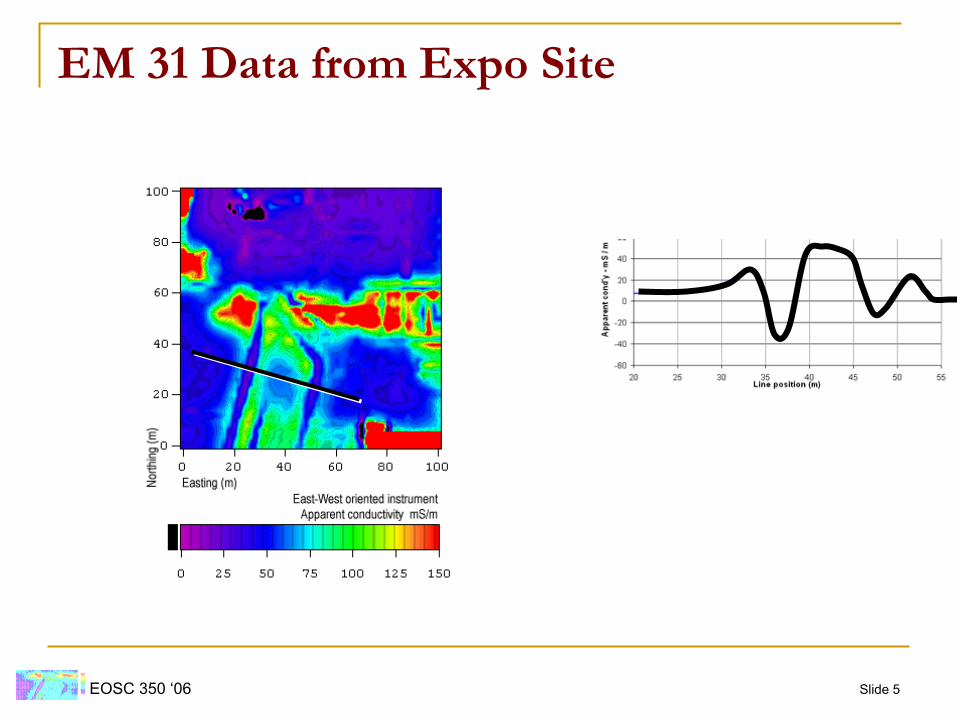
EM 31 Data from Expo Site

Electromagnetics

dtdB / E

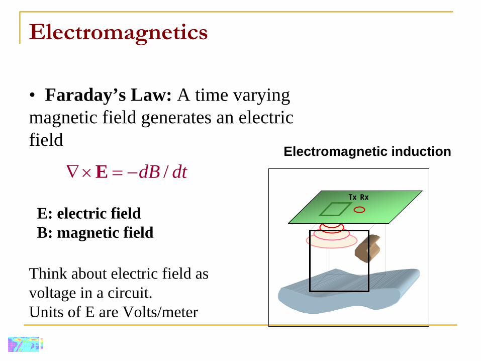
• Faraday’s Law: A time varying magnetic field generates an electric field

Tx Rx

Electromagnetic induction

E: electric fieldB: magnetic field

Think about electric field asvoltage in a circuit.Units of E are Volts/meter

Electromagnetics

JE

EJ

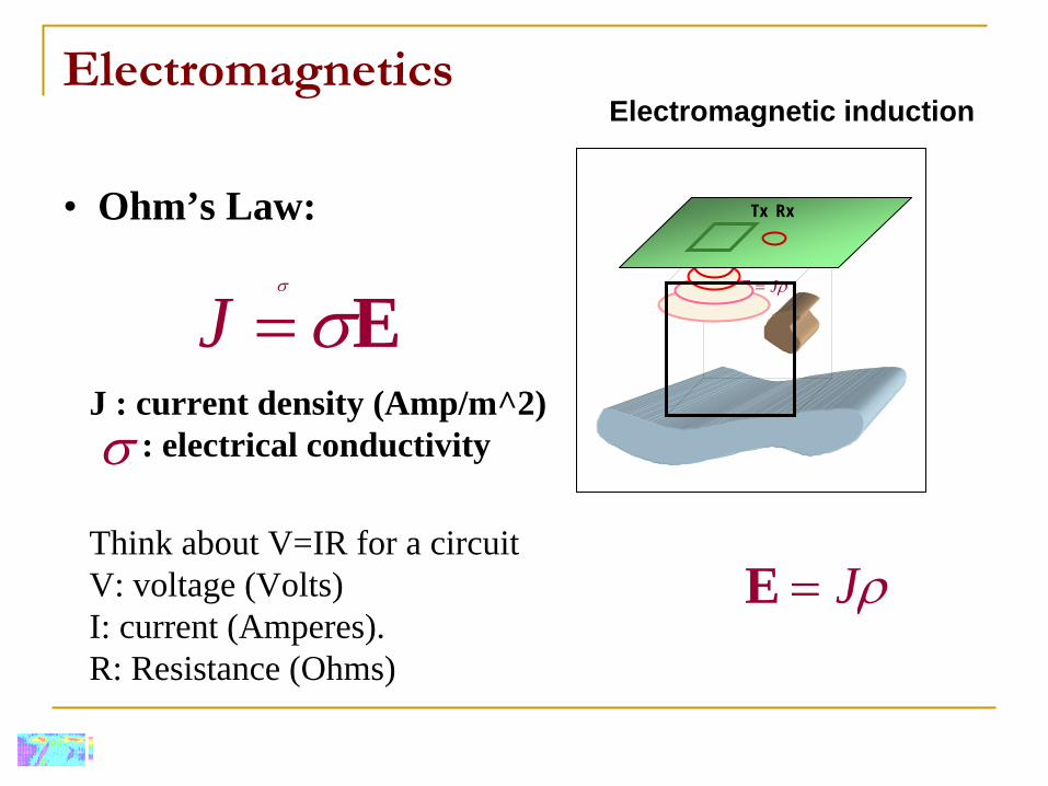
• Ohm’s Law: Tx Rx

Electromagnetic induction

J : current density (Amp/m^2): electrical conductivity

Think about V=IR for a circuitV: voltage (Volts)I: current (Amperes).R: Resistance (Ohms)

JE

EOSC 350 ‘06 Slide 8

EM induction

Faraday’s law

Time varying magnetic fields cause electric fields

Electric fields produce currents in a conductor

Hence current flows in conductors that are near an oscillating magnetic field

Electromagnetics

JH

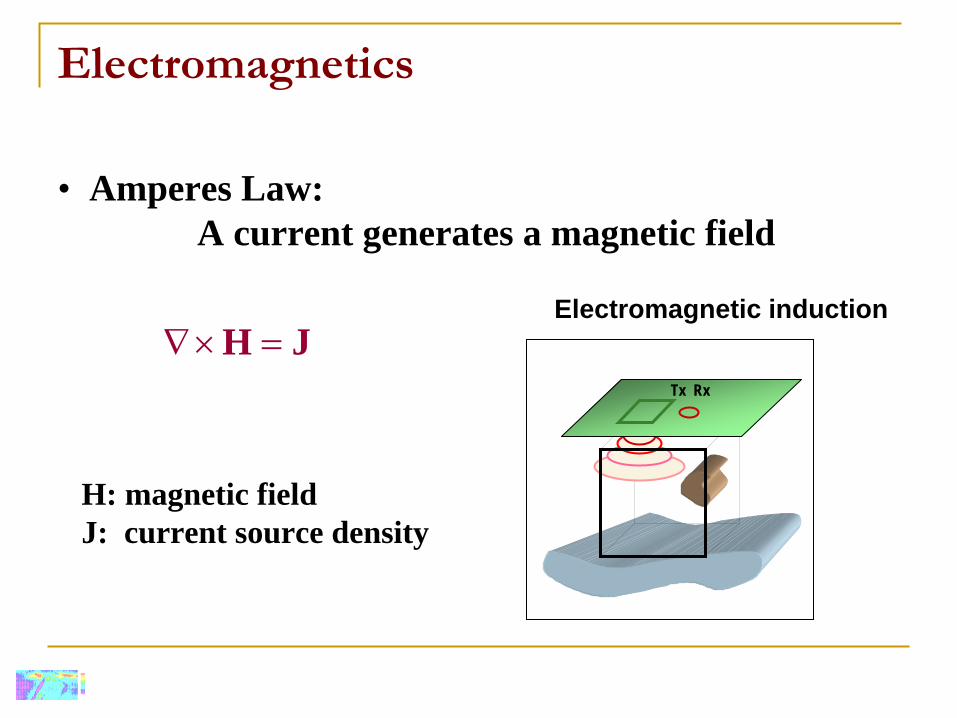
• Amperes Law: A current generates a magnetic field

Tx Rx

Electromagnetic induction

H: magnetic fieldJ: current source density

EOSC 350 ‘06 Slide 10

EM induction

Ampere’s law -

Currents generate magnetic fields

Oscillating current will cause an oscillating magnetic field

Current in wire causes a magnetic field to sur-

round it (iron filings).

Direction of the Field of a Long Straight Wire

Right Hand Rule

Grasp the wire in your right hand

Point your thumb in the direction of the current

Your fingers will curl in the direction of the field

EOSC 350 ‘06 Slide 12

EM induction

Lens’

law -

The direction of the induced currents will be in such a direction as to oppose any change in magnetic flux.

Current in wire causes a magnetic field to sur-

round it (iron filings).

Basic principles of EM induction

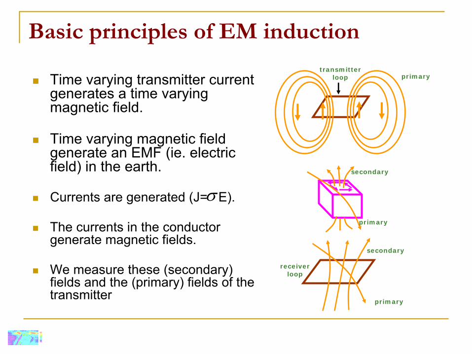
Time varying transmitter current generates a time varying magnetic field.

Time varying magnetic field generate an EMF (ie. electric field) in the earth.

Currents are generated (J= E).

The currents in the conductor generate magnetic fields.

We measure these (secondary) fields and the (primary) fields of the transmitter

primary

primary

secondary

secondary

primary

transmitter loop

receiver loop

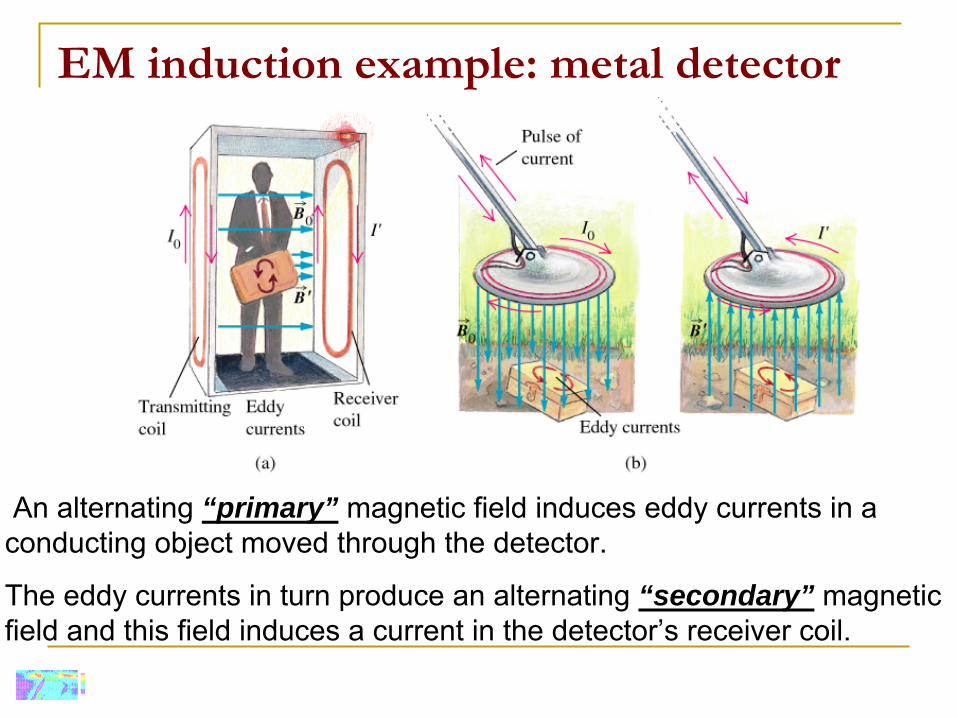
An alternating “primary” magnetic field induces eddy currents in a conducting object moved through the detector.

The eddy currents in turn produce an alternating “secondary” magnetic field and

this

field induces a current in the detector’s receiver coil.

EM induction example: metal detector

Important elements

Primary field must couple with the target

Strength of the induced currents must be big enough to generate signal

Need to choose which fields to measure

Important elements

Primary field must couple with the target

Strength of the induced currents must be big enough to generate signal

Need to choose which fields to measure

Airborne (Inductive source)

Elements of EM Induction

Transmitter and primary magnetic field

Magnetic flux and coupling

Target and induced currents

Secondary magnetic fields

Receiver

Data

Generic EM system

Tx: transmitter Rx: receiver

Tx, Rx, target body are represented as circuits

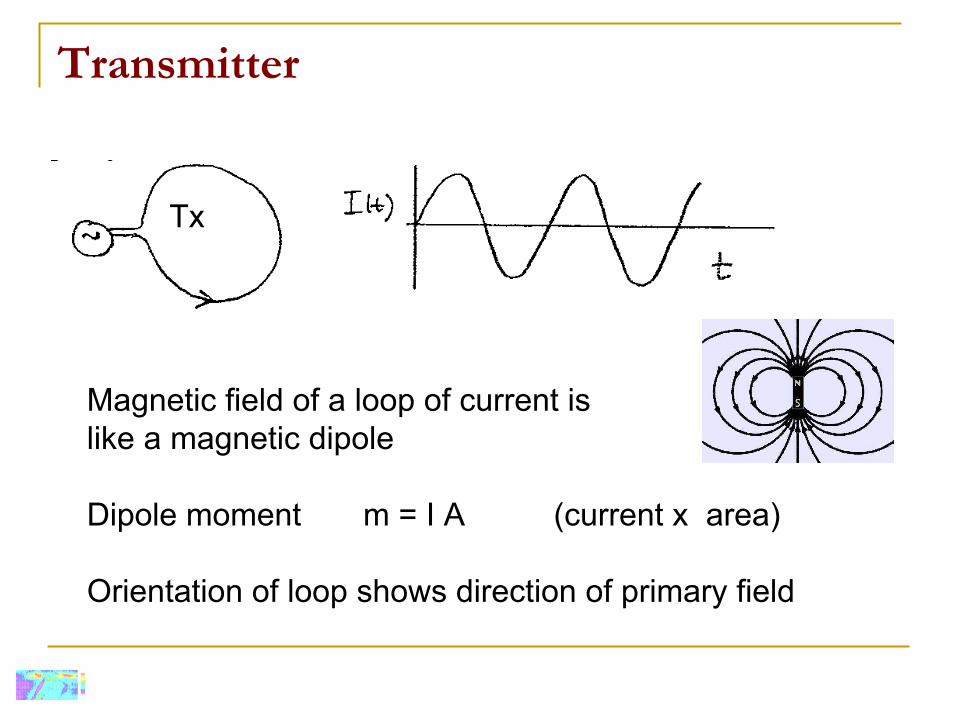
Transmitter

Magnetic field of a loop of current is like a magnetic dipole

Dipole moment m = I A (current x area)

Orientation of loop shows direction of primary field

Tx

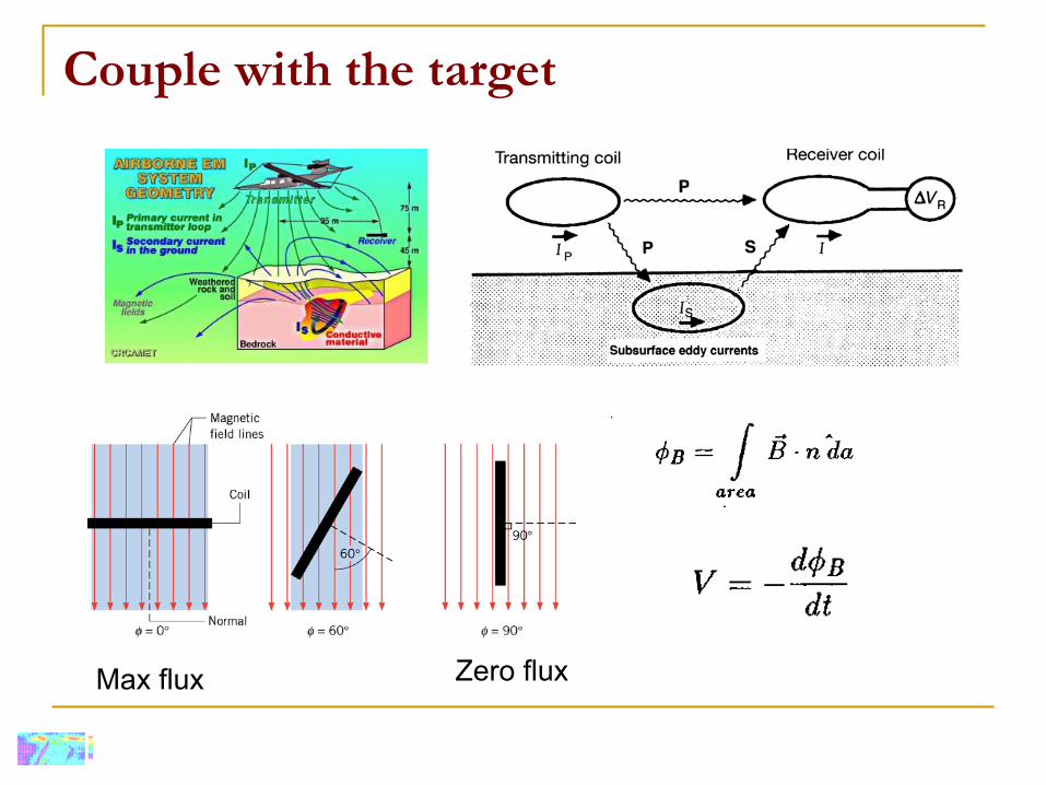
Couple with the target

Max flux Zero flux

Induced Currents in the Target

Max flux Zero flux

Think of target as an electrical circuit

Resistance R (small R means large current)

Inductance L (accounts for interaction of currents in the target

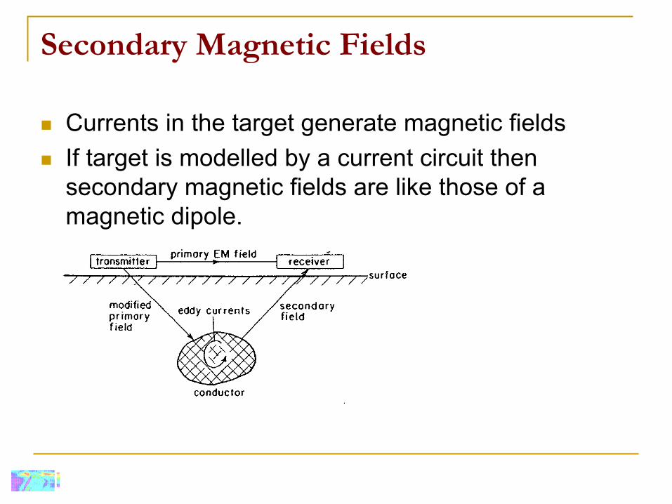
Secondary Magnetic Fields

Currents in the target generate magnetic fields

If target is modelled

by a current circuit then secondary magnetic fields are like those of a magnetic dipole.

Receiver

Receiver is a coil. A time varying flux generates a voltage.

For some instruments Hp is known and subtracted. Then receiver measures only Hs.

Frequency domain EM data

Transmitter tcos

Receiver

I(t)

V(t)

A

-A

amplitude

tAcos

Measure amplitude and phase (A, )

tAtAtA sinsincoscoscos In-phase

RealOut-of-phase

Imaginary

Or

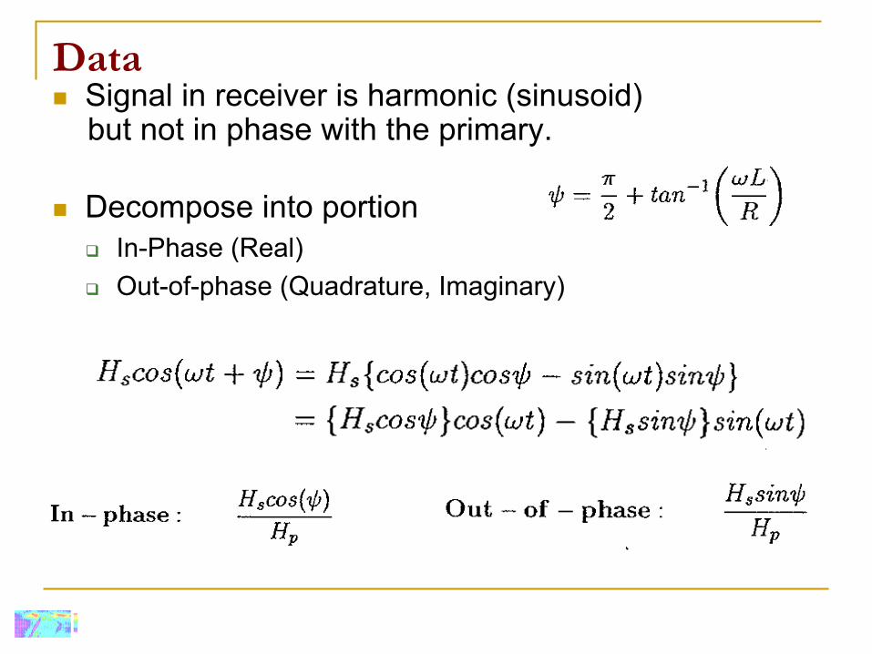
Data

Signal in receiver is harmonic (sinusoid) but not in phase with the primary.

Decompose into portion

In-Phase (Real)

Out-of-phase (Quadrature, Imaginary)

Understanding the Data

Matlab

routine to estimate the responses

fem3loop (from GPG)

demos.....

EOSC 350 ‘07 Slide 28

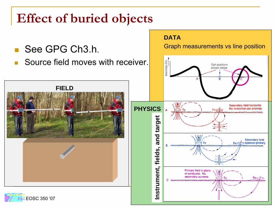
Effect of buried objects

See GPG Ch3.h.

Source field moves with receiver.

Graph measurements vs

line position

Inst

rum

ent,

field

s, a

nd ta

rget

FIELD

PHYSICS

DATA

EM Induction: Summary

Time varying magnetic magnetic

field generates an electric field E

J=σE (induced currents) (Coupling is important)

Induced currents generate secondary magnetic fields

Secondary magnetic fields are recorded at the receiver. Coupling is important.

Receiver outputs In-Phase and Out-of-phase data

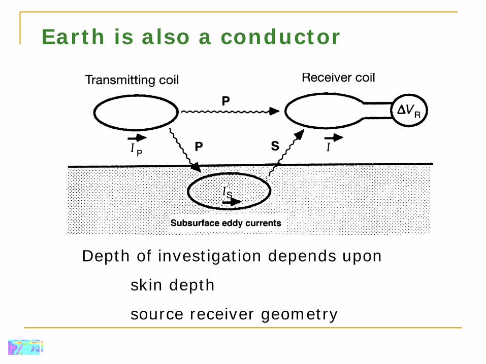
Earth is also a conductor

Depth of investigation depends upon

skin depth

source receiver geometry

EOSC 350 ‘06 Slide 31

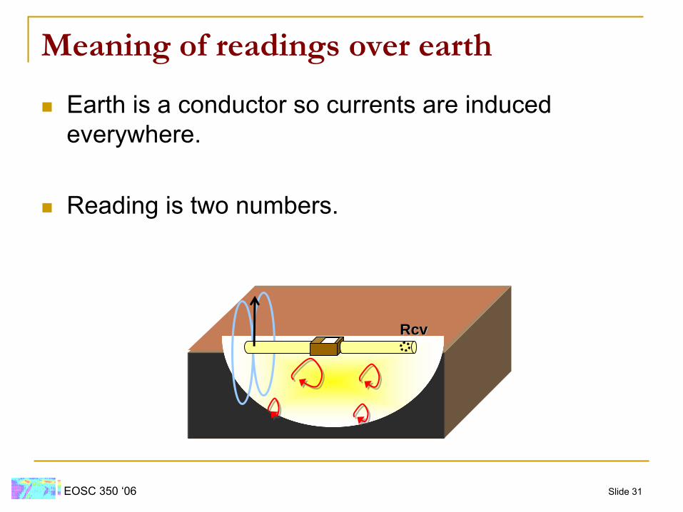
Meaning of readings over earth

Earth is a conductor so currents are induced everywhere.

Reading is two numbers.

RcvRcv

Inphase/Quadrature

The EM-31 gives two measurements called the In-phase and Quadrature

In-phase: (also called “real”)Particularly useful for find good conductors (metal pipes, drums)

Quadrature: (also called “imaginary”

or (out of phase)

Yields apparent conductivity (if s>δ)

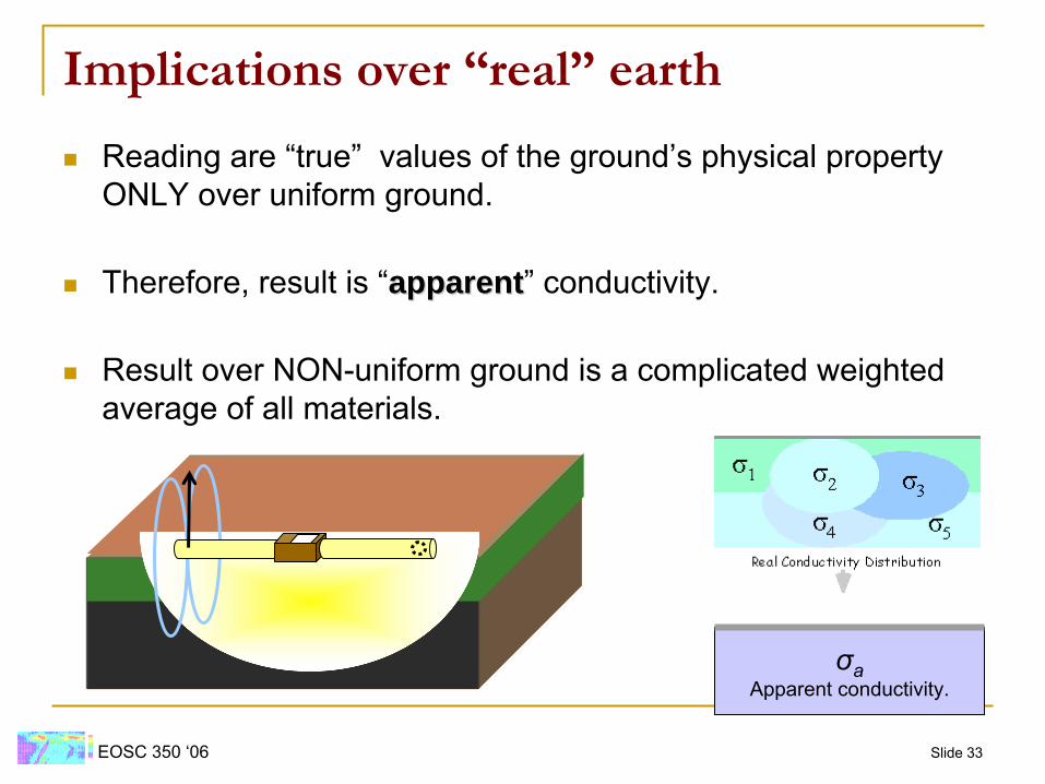
σa

Apparent conductivity.

EOSC 350 ‘06 Slide 33

Implications over “real”

earth

Reading are “true”

values of the ground’s physical property ONLY over uniform ground.

Therefore, result is “apparentapparent”

conductivity.

Result over NON-uniform ground is a complicated weighted average of all materials.

Case History Project: Expo Site

Integrated site investigation of contaminated waste site in Vancouver

Combines all the geophysical methods covered in EOSC 350: Magnetics, GPR, Seismic refraction and EM induction

EM in phase and quad phase?

EOSC 350 ‘06 Slide 38

Effect of buried objects

Contour plotted area data:

Where are peak & trough patterns?

Where are large responses?

Where are negative responses?

EM Summary so far

Basics of EM induction

Sketch approximate anomalies for a simple system (EM31) that traverses a confined body

Responses for EM31 and application

Readings for Electromagnetics

Electromagnetics

1.0 Fundamentals

GPG.h