Applications of trace estimation techniques

Shashanka Ubaru and Yousef Saad

University of Minnesota at Twin Cities, MN 55455.{ubaru001, saad}@umn.edu

Abstract. We discuss various applications of trace estimation tech-niques for evaluating functions of the form tr(f(A)) where f is certainfunction. The first problem we consider that can be cast in this form isthat of approximating the Spectral density or Density of States(DOS) ofa matrix. The DOS is a probability density distribution that measuresthe likelihood of finding eigenvalues of the matrix at a given point onthe real line, and it is an important function in solid state physicists. Wealso present a few non-standard applications of spectral densities. Othertrace estimation problems we discuss include estimating the trace of amatrix inverse tr(A−1), the problem of counting eigenvalues and esti-mating the rank, and approximating the log-determinant (trace of logfunction). We also discuss a few similar computations that arise in ma-chine learning applications. We review two computationally inexpensivemethods to compute traces of matrix functions, namely, the Chebyshevexpansion and the Lanczos Quadrature methods. A few numerical ex-amples are presented to illustrate the performances of these methods indifferent applications.

1 Introduction

Let A ∈ Rn×n be a symmetric (real) matrix with an eigen-decomposition A =UΛUT , where Λ = diag(λ1, . . . , λn), and λi, i = 1, . . . , n are the eigenvalues ofA and where the columns ui, i = 1, . . . , n of U are the associated eigenvectors.For the matrix function f(A), defined as f(A) = Uf(Λ)UT , where f(Λ) =diag(f(λ1), . . . , f(λn)) [19], the trace estimation problems consist of computingan approximation of the trace of the matrix function f(A), i.e.,

tr(f(A)) =

n∑i=1

f(λi), (1)

where λi, i = 1, . . . , n are the eigenvalues of A, and f is the desired function. Theproblem of estimating the trace of a matrix function appears in a very broadrange of applications that include machine learning, signal processing, scientificcomputing, statistics, computational biology and computational physics [5, 13,30, 28, 14, 21, 23, 2, 18]. Clearly, a trace of a matrix function can be triviallycomputed from the eigen-decomposition of A. However, matrices in most ofthe applications just mentioned are typically very large and so computing thecomplete eigen-decomposition can be expensive and sometimes even infeasible.

2

Hence, the problem is to develop fast and scalable algorithms to perform suchtasks without requiring the eigen-decomposition. This speficic problem, whichhas been at the forefront of research in many distinct areas whether in physicsor data-related applications, is the primary focus of this paper.

2 Trace estimation problems

We begin by first discussing a few trace estimation problems that arise in certainapplication areas.

2.1 Spectral Density

The first problem that we consider is that of computing the spectral density of amatrix [24], a very common problem in solid state physics. The spectral densityof matrix, also known as Density of States (DOS) in physics, is a probabilitydensity distribution that measures the likelihood of finding eigenvalues of thematrix at a given point on the real line. Formally, the spectral density of amatrix is expressed as a sum of delta functions of the eigenvalues of the matrix.That is,

φ(t) =1

n

n∑i=1

δ(t− λi),

where δ is the Dirac distribution or Dirac δ-function. This is not a proper functionbut a distribution and it is clearly not practically computable as it is defined.What is important is to compute a smoothed or approximate version of it thatdoes not require computing eigenvalues, and several inexpensive methods havebeen proposed for this purpose, [32, 36, 24]. Recently, the DOS has been used inapplications such as eigenvalue problem, e.g., for spectral slicing [39], for countingeigenvalues in intervals (‘eigencounts’) [12], and for estimating ranks [34, 35].In section 4, we present a few other (new) applications where the DOS can beexploited.

Article [24] reviews a set of inexpensive methods for computing the DOS.Here we briefly discuss two of these methods, namely the Kernel Polynomialmethod [36] and the Lanczos approximation method [24]. As was already men-tioned the DOS is not a proper function. At best it can practically be viewed as ahighly discontinuous function, which is difficult to handle numerically. The ideathen is to replace the delta function by a surrogate Gaussian blurring functionas is often done. A “blurred” version of the DOS is given by:

φσ(t) =1

n

n∑i=1

hσ(t− λi),

where hσ(t) = 1√2πσ2

e−t2

2σ2 . The spectral density can then approximated by

estimating this trace of this blurred function, e.g., using the Lanczos algorithm.An older method consists of just expanding (formally) the DOS into Chebyshevpolynomials. These two methods will be discussed later in Section 3.

3

2.2 Eigencount and Numerical Rank

The second trace estimation application we consider is that of counting eigenval-ues located in a given interval (Eigencount) and the related problem of estimat-ing the numerical rank of a matrix. Estimating the number of eigenvalues η[a,b]located in a given interval [a, b] of a large sparse symmetric matrix is a key ingre-dient of effective eigensolvers [12], because these eigensolvers require an estimateof the dimension of the eigenspace to compute to allocate resources and tune themethod under consideration. Estimating the numerical rank rε = η[ε,λ1] is an-other closely related problem that occurs in machine learning and data analysisapplications such as Principal Component Analysis (PCA), low rank approxi-mations, and reduced rank regression [34, 35]. Both of these problems can beviewed from the angle of estimating the trace of a certain eigen-projector, i.e.,the number of eigenvalues η[a, b] in [a, b] satisfies:

η[a,b] = tr(P ), where P =∑

λi ∈ [a, b]

uiu>i .

We can interpret P as a step function of A given by

P = h(A), where h(t) =

{1 if t ∈ [a, b]0 otherwise

. (2)

The problem then is to find an estimate of the trace of h(A). A few inexpensivemethods are proposed in [12, 34, 35] to approximately compute this trace. Wecan also compute the eigencount from the spectral density since

η[a, b] =

∫ b

a

∑j

δ(t− λj)dt ≡∫ b

a

nφ(t)dt. (3)

2.3 Log-determinant

Log-determinants have numerous applications in machine learning and relatedfields [30, 28, 18]. The logarithm of the determinant of a given positive definitematrix A ∈ Rn×n, is equal to the trace of the logarithm of the matrix, i.e.,

log det(A) = tr(log(A)) =

n∑i=1

log(λi).

So, estimating the log-determinant of a matrix leads once more to the estimationof the trace of a matrix function in this case the logarithm function.

Various methods have been proposed for inexpensively computing log-determinants.These methods differ in the approach used to approximate the log function. Forexample, the article [18] uses Chebyshev polynomial approximations of the logfunction, while [40, 8] uses Taylor series expansions. On the other hand, Auneet. al [3] developed a method based on rational approximations of the logarithm.Least squares approximations by polynomials have also been proposed in [10].

4

More recently, a method based on Lanczos Quadrature has been advocated forcomputing log determinants [33].Log-likelihood estimation: One of the applications of log-determinants com-putation is in the in likelihood estimation problems that arise in Gaussian pro-cesses [28]. Maximum Likelihood Estimation (MLE) is a popular approach usedfor parameter estimation in high dimensional Gaussian models. The objective isto maximize the log-likelihood function with respect to a hyperparameter vectorξ:

log p(z | ξ) = −1

2z>S(ξ)−1z − 1

2log detS(ξ)− n

2log(2π), (4)

where z is the data vector and S(ξ) is the covariance matrix parameterized byξ. As seen from the above expression, a log-determinant must be computed toobtain the log-likelihood, see [33].

2.4 Other Applications

Other frequent matrix function trace estimation problems include estimating thetrace of a matrix inverse, the Schatten norms, and the Estrada index. These arediscussed in turn.Trace of a matrix inverse: The matrix inverse trace estimation problemamounts to computing the trace of the inverse function f(t) = t−1 of a posi-tive definite matrix A ∈ Rn×n, whose eigenvalues lie in the interval [λmin, λmax]with λmin > 0. This problem appears in uncertainty quantification and in latticequantum chromodynamics [21, 38], where it is necessary to estimate the traceof the inverse of covariance matrices.Schatten p-norms: Given an input matrix X ∈ Rd×n, the Schatten p-norm of

X is defined as ‖X‖p =

(∑ri=1 σ

pi

)1/p

i, where the σi’s are the singular values

of X and r its rank. The nuclear norm is the Schatten 1-norm so it is just thesum of the singular values. Estimating the nuclear norm and the Schatten p-norms of large matrices appears in matrix completion and in rank-constrainedoptimization problems, differential privacy and theoretical chemistry [33, 26]. Itis also used in SVD entropy computations [1] which has many applications [26].Suppose we define a positive semidefinite matrix A as1 A = X>X or A = XX>.Then, the Schatten p-norm of X is defined as

‖X‖p =

( r∑i=1

λp/2i

)1/p

= tr(Ap/2).

Hence, Schatten p-norms (the nuclear norm being a special case with p = 1)are the traces of matrix functions of A with f(t) = tp/2, and they can be com-puted inexpensively using methods such as Lanczos Quadrature [33], Chebyshevexpansions [17] and others [26].

1 The matrix product is not formed explicitly since the methods involved typicallyrequire only matrix vector products.

5

Estrada index: The Estrada index of graphs is a common tool in computationalbiology, and has applications that include protein indexing [13], statistical ther-modynamics and information theory [9]. Estimating the Estrada index amountsto finding an approximation to the trace of the exponential function, i.e., weneed to estimate tr(exp(A)), where A is the adjacency matrix of the graph.Articles [17, 33, 26] discuss methods for a fast estimation of the Estrada indexof graphs.

3 Methods

We now discuss two inexpensive techniques for estimating traces of matrix func-tions. The first approach is well-known among solid-state physicists. Termed‘Kernel Polynomial Method’ (KPM) [37, 36, 35] or ‘Chebyshev expansion method’ [18,17, 34], it consists simply of expanding the spectral density into Chebyshev poly-nomials. The second approach is based on the Lanczos algorithm [24], where therelation between the Lanczos procedure and Gaussian quadrature formulas isexploited to construct a good approximation for the matrix function. We firstdiscuss a standard tool known as the ‘stochastic trace estimator’, which is a keyingredient used in the methods to be discussed.

3.1 Stochastic Trace Estimator

The stochastic trace estimator [20, 4, 29] approximates the trace of a matrixfunction f(A) by means of matrix-vector products with f(A). This method takesa sequence of random vectors vl, l = 1, ..,nv whose mean is equal to zero andwhose unit 2-norm is one, ‖vl‖2 = 1 and it then computes the average over thesamples of v>l f(A)vl to approximate the trace,

tr(f(A)) ≈ n

nv

nv∑l=1

v>l f(A)vl. (5)

Convergence has been analyzed in [4, 29]. A variant of this method can be used toestimate the diagonal diag(f(A)), see [7]. Note that f(A) need not be explicitlyformed since we only need to efficiently compute the vectors f(A)vl for any vl.This can be accomplished in a number of effective ways.

3.2 Chebyshev (Kernel) Polynomial method

The Kernel Polynomial Method (KPM) proposed in [31, 36] computes an ap-proximate DOS of a matrix using Chebyshev polynomial expansions, see, [24] fora discussion. In KPM, the matrix is linearly transformed so as to map its eigen-values from the initial interval [λn, λ1] into the interval [−1, 1]. This requiresestimating the extreme eigenvalues, see [35]. KPM seek the expansion of :

φ(t) =√

1− t2φ(t) =√

1− t2 × 1

n

n∑j=1

δ(t− λj),

6

instead of the original φ(t) since the Chebyshev polynomials are orthogonal withrespect to the weight function (1− t2)−1/2. Then, we write the partial expansion

of φ(t) as

φ(t) ≈m∑k=0

µkTk(t),

where Tk(t) is the Chebyshev polynomial of degree k. A little calculation re-veals that, formally at least, each expansion coefficient µk is given by µk =(2−δk0)

π tr(Tk(A)). Here δij is the Kronecker symbol, so 2− δk0 is 1 when k = 0and 2 otherwise. The trace of Tk(A) can now be estimated with the help of theexpansion coefficients the corresponding expansion coefficient µk are approxi-mated as,

µk ≈2− δk0πnv

nv∑l=1

(vl)>Tk(A)vl.

Scaling back by the weight function (1 − t2)−1/2, we obtain the approximationfor the spectral density function in terms of Chebyshev polynomial of degree m.

General function f(A): For a general function f : [−1, 1]→ R, it is possibleto obtain an approximation of the form

f(t) ≈m∑k=0

γkTk(t).

using Chebyshev polynomial expansions or interpolations, see [25] for details.Here Tk(t) is the Chebyshev polynomial of degree k and γk are correspondingcoefficients specific to expanding the function f(t). Hence, we can approximatethe trace of f(A) as

tr(f(A)) ≈ n

nv

nv∑l=1

[m∑k=0

γk(vl)TTk(B)vl

], (6)

using the Chebyshev expansions and the stochastic trace estimator (5). Arti-cles [12, 34] discussed the expansion of step functions using Chebyshev polyno-mials to compute eigencounts and numerical ranks of matrices, respectively.

Han et. al [17] discussed the above Chebyshev expansion method to approx-imately estimate the traces tr(f(A)), when the function f is analytic over aninterval. They proposed using Chebyshev interpolations to obtain the coeffi-cients γk. Problems such as estimating log-determinants, Estrada index, traceof matrix inverse and Shcatten p norms were discussed. Note that the functionslog(t), exp(t), t−1 and tp/2 are all analytic in the spectrum interval [λmin, λmax],with λmin > 0.

When expanding discontinuous functions including the DOS and step func-tions using Chebyshev polynomials, oscillations known as Gibbs Oscillationsappear near the discontinuities [12]. To reduce or suppress these oscillations,damping multipliers are often used, see [24, 12] for details. An important prac-tical consideration is that we can economically compute vectors of the form

7

Tk(A)v using the three term recurrence of Chebyshev polynomials, see [35, 17].The recent article [17] analyzed the convergence of methods for approximatingtr(f(A)) with the Chebyshev method when the function f(A) is analytic overthe interval of interest.

3.3 Lanczos Quadrature

The Lanczos Quadrature method was developed in [15], and the idea of combin-ing the stochastic trace estimator with the Lanczos Quadrature method appearedin [5, 6]. This method was recently analyzed and applied to matrix function traceestimation in [33]. In the Stochastic Lanczos Quadrature (SLQ) method, thescalar quantities v>f(A)v in the trace estimator (5) are computed by treatingthem to Riemann-Stieltjes integral, and then using the Gauss quadrature rule toapproximate this integral. Given the eigen-decomposition A = QΛQ>, we canwrite the scalar product as Riemann-Stieltjes integral given by,

v>f(A)v = v>Qf(Λ)Q>v =

n∑i=1

f(λi)µ2i =

∫ b

a

f(t)dµ(t), (7)

where µi are the components of the vector Q>v and the measure µ(t) is apiecewise constant function defined as

µ(t) =

0, if t < a = λ1,∑i−1j=1 µ

2j , if λi−1 ≤ t < λi, i = 2, . . . , n,∑n

j=1 µ2j , if b = λn ≤ t,

(8)

with λi ordered nondecreasingly. Next, the integral is estimated using the Gaussquadrature rule [16] ∫ b

a

f(t)dµ(t) ≈m∑k=0

ωkf(θk), (9)

where {ωk} are the weights and {θk} are the nodes of the (m+ 1)-point Gaussquadrature, which are computed using the Lanczos algorithm [14].

Given symmetric matrix A ∈ Rn×n and a starting vector w0 of unit 2-norm,the Lanczos algorithm generates an orthonormal basis Wm+1 for the Krylovsubspace Span{w0, Aw0, . . . , A

mw0} such that W>m+1AWm+1 = Tm+1, whereTm+1 is an (m+ 1)× (m+ 1) tridiagonal matrix. The columns wk of Wm+1 arerelated as

wk = pk−1(A)w0, k = 1, . . . ,m,

where pk are the Lanczos polynomials. The Lanczos polynomials are orthogonalwith respect to the measure µ(t) in (8); see Theorem 4.2 in [14]. The nodes andthe weights of the quadrature rule in (9) can be computed as the eigenvaluesand the squares of the first entries of the eigenvectors of Tm+1. Thus, we have

v>f(A)v ≈m∑k=0

τ2kf(θk) with τ2k =[e>1 yk

]2, (10)

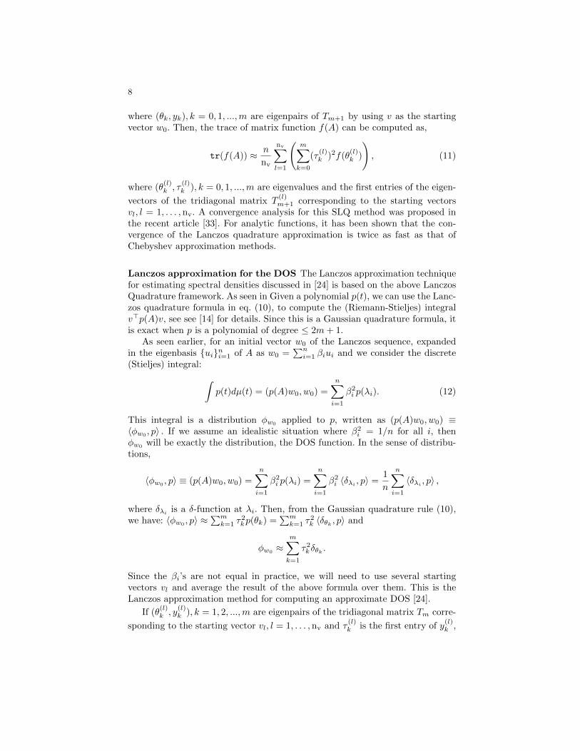
8

where (θk, yk), k = 0, 1, ...,m are eigenpairs of Tm+1 by using v as the startingvector w0. Then, the trace of matrix function f(A) can be computed as,

tr(f(A)) ≈ n

nv

nv∑l=1

(m∑k=0

(τ(l)k )2f(θ

(l)k )

), (11)

where (θ(l)k , τ

(l)k ), k = 0, 1, ...,m are eigenvalues and the first entries of the eigen-

vectors of the tridiagonal matrix T(l)m+1 corresponding to the starting vectors

vl, l = 1, . . . ,nv. A convergence analysis for this SLQ method was proposed inthe recent article [33]. For analytic functions, it has been shown that the con-vergence of the Lanczos quadrature approximation is twice as fast as that ofChebyshev approximation methods.

Lanczos approximation for the DOS The Lanczos approximation techniquefor estimating spectral densities discussed in [24] is based on the above LanczosQuadrature framework. As seen in Given a polynomial p(t), we can use the Lanc-zos quadrature formula in eq. (10), to compute the (Riemann-Stieljes) integralv>p(A)v, see see [14] for details. Since this is a Gaussian quadrature formula, itis exact when p is a polynomial of degree ≤ 2m+ 1.

As seen earlier, for an initial vector w0 of the Lanczos sequence, expandedin the eigenbasis {ui}ni=1 of A as w0 =

∑ni=1 βiui and we consider the discrete

(Stieljes) integral: ∫p(t)dµ(t) = (p(A)w0, w0) =

n∑i=1

β2i p(λi). (12)

This integral is a distribution φw0 applied to p, written as (p(A)w0, w0) ≡〈φw0 , p〉 . If we assume an idealistic situation where β2

i = 1/n for all i, thenφw0

will be exactly the distribution, the DOS function. In the sense of distribu-tions,

〈φw0 , p〉 ≡ (p(A)w0, w0) =

n∑i=1

β2i p(λi) =

n∑i=1

β2i 〈δλi , p〉 =

1

n

n∑i=1

〈δλi , p〉 ,

where δλi is a δ-function at λi. Then, from the Gaussian quadrature rule (10),we have: 〈φw0 , p〉 ≈

∑mk=1 τ

2kp(θk) =

∑mk=1 τ

2k 〈δθk , p〉 and

φw0 ≈m∑k=1

τ2k δθk .

Since the βi’s are not equal in practice, we will need to use several startingvectors vl and average the result of the above formula over them. This is theLanczos approximation method for computing an approximate DOS [24].

If (θ(l)k , y

(l)k ), k = 1, 2, ...,m are eigenpairs of the tridiagonal matrix Tm corre-

sponding to the starting vector vl, l = 1, . . . ,nv and τ(l)k is the first entry of y

(l)k ,

9

then the DOS function by Lanczos approximation is given by

φ(t) =1

nv

nv∑l=1

(m∑k=1

(τ(l)k )2δ(t− θ(l)k )

). (13)

The above function is a weighted spectral distribution of Tm, where τ2k is theweight for the corresponding eigenvalue θk and it approximates the spectraldensity of A.

Computational Cost: The most expensive step in KPM is when computingthe scalars (vl)

>Tk(A)vl for l = 1, . . . ,nv, k = 0, . . . ,m. Hence, the computa-tional cost for estimating traces of matrix functions by KPM will beO(nnz(A)mnv)for sparse matrices, where nnz(A) is the number of nonzero entries of A. Simi-larly, the most expensive part of the Lanczos Quadrature procedure is to performthe m Lanczos steps with the different starting vectors. The computational costfor matrix function trace estimation by SLQ will be O((nnz(A)m+nm2)nv) forsparse matrices where there is an assumed cost for reorthogonalizing the Lanczosvectors. As can be seen, these algorithms are inexpensive relative to methodsthat require matrix factorizations such as the QR or SVD.

4 Applications of the DOS

Among the applications of the DOS that were mentioned earlier, we will discusstwo that are somewhat related. The first is a tool employed for estimating therank of a matrix. This is only briefly sketched as it has been discussed in detailsearlier in [34, 35]. The second application, is in clustering and the problem ofcommunity detection in social graphs.

Threshold selection for rank estimation: The numerical rank of a generalmatrix X ∈ Rd×n is defined with respect to a positive tolerance ε as follows:

rε = min{rank(B) : B ∈ Rd×n, ‖X −B‖2 ≤ ε}. (14)

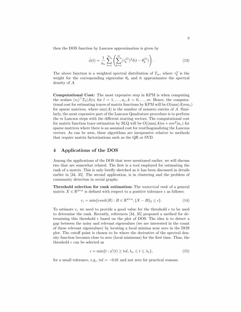
To estimate rε we need to provide a good value for the threshold ε to be usedto determine the rank. Recently, references [34, 35] proposed a method for de-termining this threshold ε based on the plot of DOS. The idea is to detect agap between the noisy and relevant eigenvalues (we are interested in the countof these relevant eigenvalues) by locating a local minima near zero in the DOSplot. The cutoff point is chosen to be where the derivative of the spectral den-sity function becomes close to zero (local minimum) for the first time. Thus, thethreshold ε can be selected as

ε = min{t : φ′(t) ≥ tol, λn ≤ t ≤ λ1}, (15)

for a small tolerance, e.g., tol = −0.01 and not zero for practical reasons.

10

0 100 200 300 400 500 600 700 800 900

0

100

200

300

400

500

600

700

800

900

nz = 58026

0 20 40 60 80 100 120

0

20

40

60

80

100

120

nz = 3750

0.1 0.2 0.3 0.4 0.5 0.6 0.7

0

0.05

0.1

0.15

0.2

λ

φ

DOS (Lanczos)

DOS plot by Lanczos m=50

(λ)

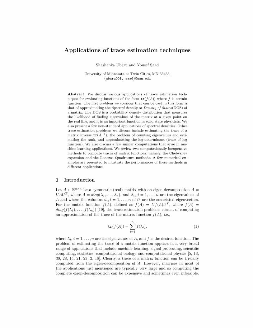
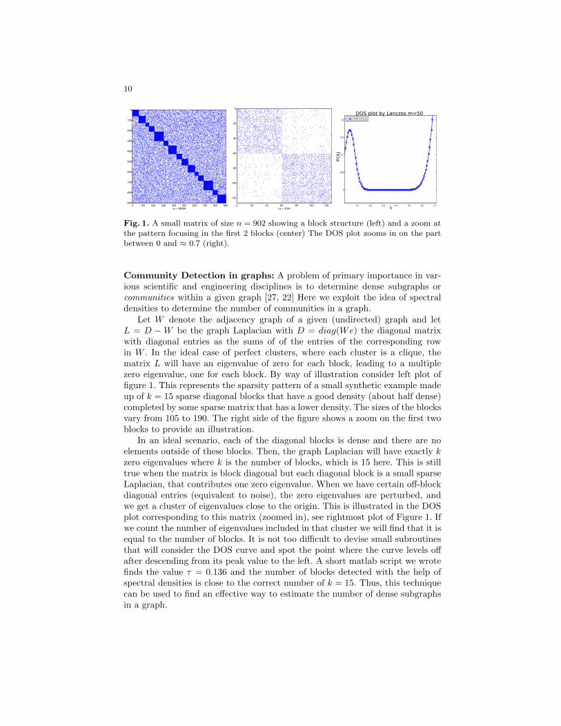
Fig. 1. A small matrix of size n = 902 showing a block structure (left) and a zoom atthe pattern focusing in the first 2 blocks (center) The DOS plot zooms in on the partbetween 0 and ≈ 0.7 (right).

Community Detection in graphs: A problem of primary importance in var-ious scientific and engineering disciplines is to determine dense subgraphs orcommunities within a given graph [27, 22] Here we exploit the idea of spectraldensities to determine the number of communities in a graph.

Let W denote the adjacency graph of a given (undirected) graph and letL = D −W be the graph Laplacian with D = diag(We) the diagonal matrixwith diagonal entries as the sums of of the entries of the corresponding rowin W . In the ideal case of perfect clusters, where each cluster is a clique, thematrix L will have an eigenvalue of zero for each block, leading to a multiplezero eigenvalue, one for each block. By way of illustration consider left plot offigure 1. This represents the sparsity pattern of a small synthetic example madeup of k = 15 sparse diagonal blocks that have a good density (about half dense)completed by some sparse matrix that has a lower density. The sizes of the blocksvary from 105 to 190. The right side of the figure shows a zoom on the first twoblocks to provide an illustration.

In an ideal scenario, each of the diagonal blocks is dense and there are noelements outside of these blocks. Then, the graph Laplacian will have exactly kzero eigenvalues where k is the number of blocks, which is 15 here. This is stilltrue when the matrix is block diagonal but each diagonal block is a small sparseLaplacian, that contributes one zero eigenvalue. When we have certain off-blockdiagonal entries (equivalent to noise), the zero eigenvalues are perturbed, andwe get a cluster of eigenvalues close to the origin. This is illustrated in the DOSplot corresponding to this matrix (zoomed in), see rightmost plot of Figure 1. Ifwe count the number of eigenvalues included in that cluster we will find that it isequal to the number of blocks. It is not too difficult to devise small subroutinesthat will consider the DOS curve and spot the point where the curve levels offafter descending from its peak value to the left. A short matlab script we wrotefinds the value τ = 0.136 and the number of blocks detected with the help ofspectral densities is close to the correct number of k = 15. Thus, this techniquecan be used to find an effective way to estimate the number of dense subgraphsin a graph.

11

0 100 200 300 400 500 600 700 800−5

0

5

10

15

20

25

30

35

40

45

Eige

nval

ue λ

i

i −−>

Matrix Spectrum

5 10 15 20 25 30 35 40

0.005

0.01

0.015

0.02

0.025

0.03

0.035

0.04

0.045

KPM by Chebyshev polynomials, deg = 50Hist

φλ(

(

λ

KPM Jackson damping

0 5 10 15 20 25 30 35 400

0.005

0.01

0.015

0.02

0.025

0.03

0.035

0.04

0.045

DOS by 50 step Lanczos w. gaussian blurring

HistLanczos

φ

λ

λ(

(

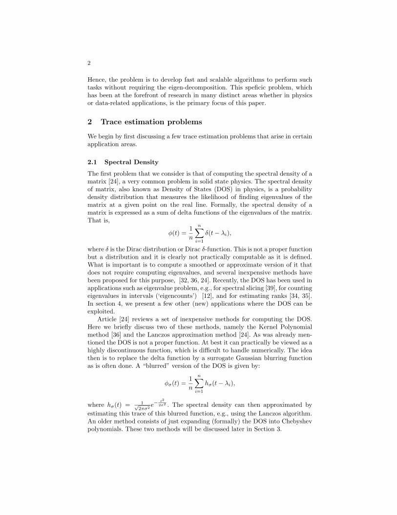
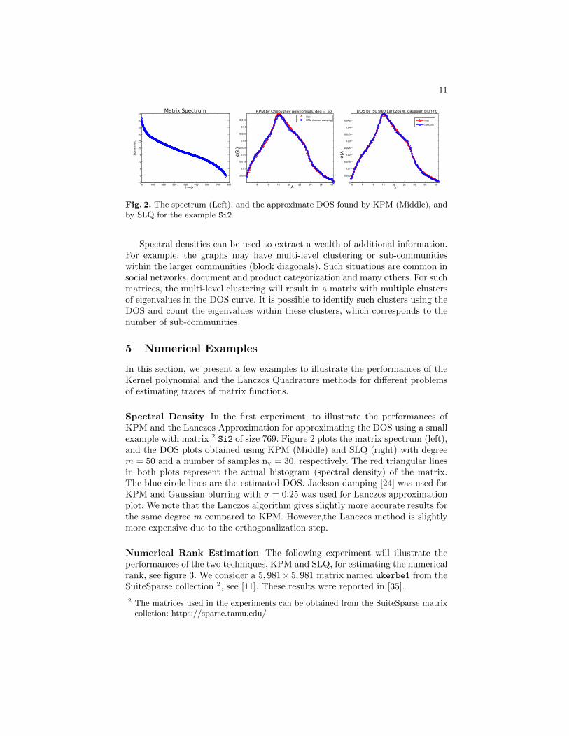
Fig. 2. The spectrum (Left), and the approximate DOS found by KPM (Middle), andby SLQ for the example Si2.

Spectral densities can be used to extract a wealth of additional information.For example, the graphs may have multi-level clustering or sub-communitieswithin the larger communities (block diagonals). Such situations are common insocial networks, document and product categorization and many others. For suchmatrices, the multi-level clustering will result in a matrix with multiple clustersof eigenvalues in the DOS curve. It is possible to identify such clusters using theDOS and count the eigenvalues within these clusters, which corresponds to thenumber of sub-communities.

5 Numerical Examples

In this section, we present a few examples to illustrate the performances of theKernel polynomial and the Lanczos Quadrature methods for different problemsof estimating traces of matrix functions.

Spectral Density In the first experiment, to illustrate the performances ofKPM and the Lanczos Approximation for approximating the DOS using a smallexample with matrix 2 Si2 of size 769. Figure 2 plots the matrix spectrum (left),and the DOS plots obtained using KPM (Middle) and SLQ (right) with degreem = 50 and a number of samples nv = 30, respectively. The red triangular linesin both plots represent the actual histogram (spectral density) of the matrix.The blue circle lines are the estimated DOS. Jackson damping [24] was used forKPM and Gaussian blurring with σ = 0.25 was used for Lanczos approximationplot. We note that the Lanczos algorithm gives slightly more accurate results forthe same degree m compared to KPM. However,the Lanczos method is slightlymore expensive due to the orthogonalization step.

Numerical Rank Estimation The following experiment will illustrate theperformances of the two techniques, KPM and SLQ, for estimating the numericalrank, see figure 3. We consider a 5, 981× 5, 981 matrix named ukerbe1 from theSuiteSparse collection 2, see [11]. These results were reported in [35].

2 The matrices used in the experiments can be obtained from the SuiteSparse matrixcolletion: https://sparse.tamu.edu/

12

0 1000 2000 3000 4000 5000 60000

1

2

3

4

5

6

7

8

9

10

λ i

i

Matrix Spectrum

0 20 40 603800

4000

4200

4400

4600

4800Chebyshev Polynomial nv=30 (size=5981)

Degree (5 −> 50)

Estimed

#eigenvaluesininterval

Cumulative AvgvTf(A)vExact

0 20 40 603700

3800

3900

4000

4100

4200Lanczos Approximation nv=30 (size=5981)

Degree (5 −> 50)

Estimed

#eigenvaluesininterval

Cumulative Avg

vTf(A)vExact

0 1 2 3 4 5 6 7 8 9 100

0.05

0.1

0.15

0.2

0.25

0.3

0.35DOS with KPM, deg M = 50

λ

φ(λ

)

0 10 20 303900

3950

4000

4050

4100

4150

4200Polynomial method (matrix size=5981)

Number of vectors (1 −> 30)

Estim

ed#eige

nvalue

sin

interval

CumulativeAvg(rε)ℓExact

0 10 20 303900

3950

4000

4050

4100

4150Lanczos Approximation (matrix size=5981)

Number of vectors (1 −> 30)

Estimed

#eigenvaluesininterval

CumulativeAvg(rε)ℓExact

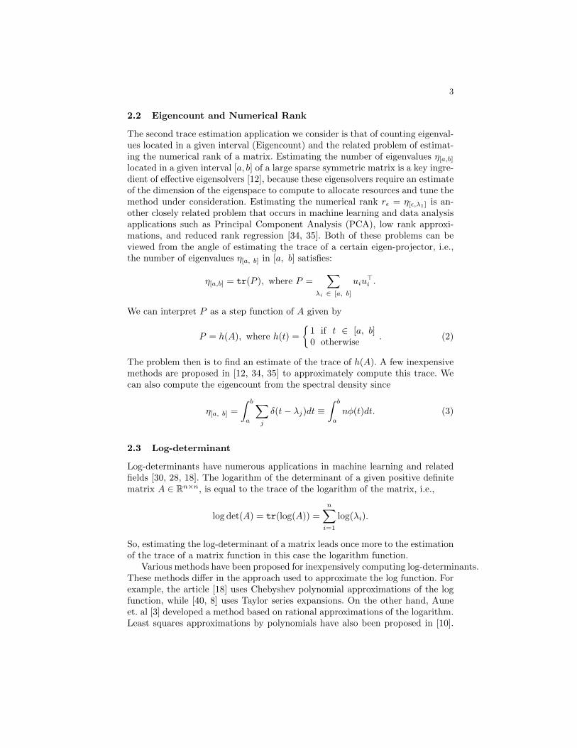
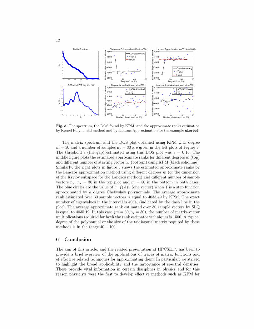
Fig. 3. The spectrum, the DOS found by KPM, and the approximate ranks estimationby Kernel Polynomial method and by Lanczos Approximation for the example ukerbe1.

The matrix spectrum and the DOS plot obtained using KPM with degreem = 50 and a number of samples nv = 30 are given in the left plots of Figure 3.The threshold ε (the gap) estimated using this DOS plot was ε = 0.16. Themiddle figure plots the estimated approximate ranks for different degrees m (top)and different number of starting vector nv (bottom) using KPM (black solid line).Similarly, the right plots in figure 3 shows the estimated approximate ranks bythe Lanczos approximation method using different degrees m (or the dimensionof the Krylov subspace for the Lanczos method) and different number of samplevectors nv. nv = 30 in the top plot and m = 50 in the bottom in both cases.The blue circles are the value of v>f(A)v (one vector) when f is a step functionapproximated by k degree Chebyshev polynomials. The average approximaterank estimated over 30 sample vectors is equal to 4033.49 by KPM. The exactnumber of eigenvalues in the interval is 4034, (indicated by the dash line in theplot). The average approximate rank estimated over 30 sample vectors by SLQis equal to 4035.19. In this case (m = 50,nv = 30), the number of matrix-vectormultiplications required for both the rank estimator techniques is 1500. A typicaldegree of the polynomial or the size of the tridiagonal matrix required by thesemethods is in the range 40− 100.

6 Conclusion

The aim of this article, and the related presentation at HPCSE17, has been toprovide a brief overview of the applications of traces of matrix functions andof effective related techniques for approximating them. In particular, we strivedto highlight the broad applicability and the importance of spectral densities.These provide vital information in certain disciplines in physics and for thisreason physicists were the first to develop effective methods such as KPM for

13

computing them. On the other hand, the use of spectral densities, and moregenerally traces of matrix functions, in other areas such as machine learning andcomputational statistics, is more recent. There is no doubt that the interest inthis topic will gain in importance given the rapid progress of disciplines thatexploit large datasets.

Acknowledgments. This work was supported by NSF under grant CCF-1318597.

Bibliography

[1] O. Alter, P. O. Brown, and D. Botstein. Singular value decomposition forgenome-wide expression data processing and modeling. Proceedings of the Na-tional Academy of Sciences, 97(18):10101–10106, 2000.

[2] A. Andoni, R. Krauthgamer, and I. Razenshteyn. Sketching and embedding areequivalent for norms. In Proceedings of the Forty-Seventh Annual ACM on Sym-posium on Theory of Computing, pages 479–488. ACM, 2015.

[3] E. Aune, D. P. Simpson, and J. Eidsvik. Parameter estimation in high dimensionalGaussian distributions. Statistics and Computing, 24(2):247–263, 2014.

[4] H. Avron and S. Toledo. Randomized algorithms for estimating the trace of animplicit symmetric positive semi-definite matrix. Journal of the ACM, 58(2):8,2011.

[5] Z. Bai, G. Fahey, and G. Golub. Some large-scale matrix computation problems.Journal of Computational and Applied Mathematics, 74(1):71–89, 1996.

[6] Z. Bai and G. H. Golub. Bounds for the trace of the inverse and the determinant ofsymmetric positive definite matrices. Annals of Numerical Mathematics, 4:29–38,1996.

[7] C. Bekas, E. Kokiopoulou, and Y. Saad. An estimator for the diagonal of a matrix.Applied numerical mathematics, 57(11):1214–1229, 2007.

[8] C. Boutsidis, P. Drineas, P. Kambadur, E.-M. Kontopoulou, and A. Zouzias. Arandomized algorithm for approximating the log determinant of a symmetric pos-itive definite matrix. Linear Algebra and its Applications, 533:95–119, 2017.

[9] R. Carbo-Dorca. Smooth function topological structure descriptors based ongraph-spectra. Journal of Mathematical Chemistry, 44(2):373–378, 2008.

[10] J. Chen, M. Anitescu, and Y. Saad. Computing f(a)b via least squares polynomialapproximations. SIAM Journal on Scientific Computing, 33(1):195–222, 2011.

[11] T. A. Davis and Y. Hu. The University of Florida sparse matrix collection. ACMTransactions on Mathematical Software (TOMS), 38(1):1, 2011.

[12] E. Di Napoli, E. Polizzi, and Y. Saad. Efficient estimation of eigenvalue counts inan interval. ArXiv preprint ArXiv:1308.4275, 2013.

[13] E. Estrada. Characterization of 3d molecular structure. Chemical Physics Letters,319(5):713–718, 2000.

[14] G. H. Golub and G. Meurant. Matrices, moments and quadrature with applica-tions. Princeton University Press, 2009.

[15] G. H. Golub and Z. Strakos. Estimates in quadratic formulas. Numerical Algo-rithms, 8(2):241–268, 1994.

[16] G. H. Golub and J. H. Welsch. Calculation of gauss quadrature rules. Mathematicsof Computation, 23(106):221–230, 1969.

[17] I. Han, D. Malioutov, H. Avron, and J. Shin. Approximating spectral sums oflarge-scale matrices using stochastic chebyshev approximations. SIAM Journalon Scientific Computing, 39(4):A1558–A1585, 2017.

[18] I. Han, D. Malioutov, and J. Shin. Large-scale log-determinant computationthrough stochastic chebyshev expansions. In Proceedings of The 32nd Interna-tional Conference on Machine Learning, pages 908–917, 2015.

[19] N. J. Higham. Functions of matrices: theory and computation. SIAM, 2008.

15

[20] M. F. Hutchinson. A stochastic estimator of the trace of the influence matrixfor Laplacian smoothing splines. Communications in Statistics-Simulation andComputation, 19(2):433–450, 1990.

[21] V. Kalantzis, C. Bekas, A. Curioni, and E. Gallopoulos. Accelerating data un-certainty quantification by solving linear systems with multiple right-hand sides.Numerical Algorithms, 62(4):637–653, 2013.

[22] L. Kaufman and P. J. Rousseeuw. Finding Groups in Data: An Introduction toCluster Analysis. John Wiley & Sons Ltd., 1990.

[23] Y. Li, H. L. Nguyen, and D. P. Woodruff. On sketching matrix norms and thetop singular vector. In Proceedings of the Twenty-Fifth Annual ACM-SIAM Sym-posium on Discrete Algorithms, pages 1562–1581. SIAM, 2014.

[24] L. Lin, Y. Saad, and C. Yang. Approximating spectral densities of large matrices.SIAM Review, 58(1):34–65, 2016.

[25] J. C. Mason and D. C. Handscomb. Chebyshev polynomials. CRC Press, 2002.[26] C. Musco, P. Netrapalli, A. Sidford, S. Ubaru, and D. P. Woodruff. Spectrum

approximation beyond fast matrix multiplication: Algorithms and hardness. arXivpreprint arXiv:1704.04163, 2017.

[27] M. E. J. Newman. Finding community structure in networks using the eigenvectorsof matrices. Physical review E, 74(3):036104, 2006.

[28] C. Rasmussen and C. Williams. Gaussian Processes for Machine Learning. MITPress, 2006.

[29] F. Roosta-Khorasani and U. Ascher. Improved bounds on sample size for implicitmatrix trace estimators. Foundations of Computational Mathematics, pages 1–26,2014.

[30] H. Rue and L. Held. Gaussian Markov random fields: theory and applications.CRC Press, 2005.

[31] R. Silver and H. Roder. Densities of states of mega-dimensional Hamiltonianmatrices. International Journal of Modern Physics C, 5(04):735–753, 1994.

[32] I. Turek. A maximum-entropy approach to the density of states within the recur-sion method. Journal of Physics C: Solid State Physics, 21(17):3251, 1988.

[33] S. Ubaru, J. Chen, and Y. Saad. Fast estimation of tr(f(A)) via stochastic Lanczosquadrature. SIAM Journal on Matrix Analysis and Applications, 2017. In Press.

[34] S. Ubaru and Y. Saad. Fast methods for estimating the numerical rank of largematrices. In Proceedings of The 33rd International Conference on Machine Learn-ing, pages 468–477, 2016.

[35] S. Ubaru, Y. Saad, and A.-K. Seghouane. Fast estimation of approximate matrixranks using spectral densities. Neural Computation, 29(5):1317–1351, 2017.

[36] L.-W. Wang. Calculating the density of states and optical-absorption spectra oflarge quantum systems by the plane-wave moments method. Physical Review B,49(15):10154, 1994.

[37] A. Weiße, G. Wellein, A. Alvermann, and H. Fehske. The kernel polynomialmethod. Reviews of modern physics, 78(1):275, 2006.

[38] L. Wu, J. Laeuchli, V. Kalantzis, A. Stathopoulos, and E. Gallopoulos. Esti-mating the trace of the matrix inverse by interpolating from the diagonal of anapproximate inverse. Journal of Computational Physics, 326:828–844, 2016.

[39] Y. Xi, R. Li, and Y. Saad. Fast computation of spectral densities for generalizedeigenvalue problems. arXiv preprint arXiv:1706.06610, 2017.

[40] Y. Zhang and W. E. Leithead. Approximate implementation of the logarithmof the matrix determinant in Gaussian process regression. journal of StatisticalComputation and Simulation, 77(4):329–348, 2007.