Computational rephotography - Agarwala · Additional Key Words and Phrases: Computational photography, pose estimation, rephotography ACM Reference Format: ... Computational Rephotography

24

Computational Rephotography

SOONMIN BAEMIT Computer Science and Artificial Intelligence LaboratoryASEEM AGARWALAAbobe Systems, Inc.andFREDO DURANDMIT Computer Science and Artificial Intelligence Laboratory

Rephotographers aim to recapture an existing photograph from the same viewpoint. A historical photograph paired with a well-aligned modern rephotographcan serve as a remarkable visualization of the passage of time. However, the task of rephotography is tedious and often imprecise, because reproducing theviewpoint of the original photograph is challenging. The rephotographer must disambiguate between the six degrees of freedom of 3D translation and rotation,and the confounding similarity between the effects of camera zoom and dolly.

We present a real-time estimation and visualization technique for rephotography that helps users reach a desired viewpoint during capture. The input to ourtechnique is a reference image taken from the desired viewpoint. The user moves through the scene with a camera and follows our visualization to reach thedesired viewpoint. We employ computer vision techniques to compute the relative viewpoint difference. We guide 3D movement using two 2D arrows. Wedemonstrate the success of our technique by rephotographing historical images and conducting user studies.

Categories and Subject Descriptors: H.5.2 [Information interfaces and Presentation (e.g., HCI)]: User Interfaces; I.4.9 [Image Processing and ComputerVision]: Applications

General Terms: Algorithms, Design, Human Factors

Additional Key Words and Phrases: Computational photography, pose estimation, rephotography

ACM Reference Format:

Bae, S., Agarwala, A., and Durand, F. 2010. Computational rephotography. ACM Trans. Graph. 29, 3, Article 24 (June 2010), 15 pages.DOI = 10.1145/1805964.1805968 http://doi.acm.org/10.1145/1805964.1805968

1. INTRODUCTION

Rephotography is the act of repeat photography; capturing a pho-tograph of the same scene from the same viewpoint of an existingphotograph that is typically much older. An image and its repho-tograph can provide a compelling “then and now” visualizationof the progress of time (Figure 1). Rephotography is a powerfultool for the study of history. Well-known examples include Sec-ond View [Klett et al. 1990] (a rephotographic survey of landscapeimages of the American West), New York Changing [Levere et al.2004], and a series of forty Then and Now books that each repho-tograph a major world city (e.g., McNulty [2002]). Beyond history,rephotography is also used to document glacier melting as evidenceof global warming [Gore 2006], and to monitor geological erosionand change [Hall 2002].

This work was supported by grants from Quanta, Shell, and Adobe.Authors’ addresses: S. Bae, MIT Computer Science and Artificial Intelligence Laboratory, MIT, 77 Massachusetts Avenue, Cambridge, MA 02139-4307; email:[email protected]; A. Agarwala, Abobe Systems, Inc.; F. Durand, MIT Computer Science and Artificial Intelligence Laboratory, MIT, 77 MassachusettsAvenue, Cambridge, MA 02139-4307.Permission to make digital or hard copies of part or all of this work for personal or classroom use is granted without fee provided that copies are not madeor distributed for profit or commercial advantage and that copies show this notice on the first page or initial screen of a display along with the full citation.Copyrights for components of this work owned by others than ACM must be honored. Abstracting with credit is permitted. To copy otherwise, to republish, topost on servers, to redistribute to lists, or to use any component of this work in other works requires prior specific permission and/or a fee. Permissions may berequested from Publications Dept., ACM, Inc., 2 Penn Plaza, Suite 701, New York, NY 10121-0701 USA, fax +1 (212) 869-0481, or [email protected]© 2010 ACM 0730-0301/2010/06-ART24 $10.00 DOI 10.1145/1805964.1805968 http://doi.acm.org/ 10.1145/1805964.1805968

When a photograph and its rephotograph match well, a digitalcross-fade between the two is a remarkable artifact; decades go byin the blink of an eye, and it becomes evident which scene ele-ments are preserved and which have changed across time. To createa faithful rephotograph, the viewpoint of the original photographmust be carefully reproduced at the moment of capture. However,as we have confirmed through a user study, exactly matching a pho-tograph’s viewpoint “by eye” is remarkably challenging; the repho-tographer must disambiguate between the six degrees of freedomof 3D translation and rotation, and, in particular, the confoundingsimilarity between the effects of camera zoom and dolly. There aredigital techniques for shifting viewpoint after capture [Kang andShum 2002], but they are still brittle and heavyweight, and dependon the solution of several classic and challenging computer visionproblems.

ACM Transactions on Graphics, Vol. 29, No. 3, Article 24, Publication date: June 2010.

24:2 • S. Bae et al.

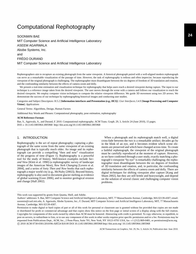
Fig. 1. Rephotography gives two views of the same place around a centuryapart. Pictures are from New York Changing [Levere et al. 2004] and BostonThen and Now [McNulty 2002].

In this article, we present an interactive, computational techniquefor rephotography that focuses on the task of matching the view-point of a reference photograph at capture time. We envision ourtool running directly on the digital camera; but since these plat-forms are currently closed and do not yet have enough processingpower, our prototype consists of a digital camera connected to alaptop. The user simply points the camera towards the scene de-picted in the reference image, and our technique estimates andvisualizes the camera motion required to reach the desired view-point in real time. Algorithmically, we build on existing computervision algorithms to compute the relative pose between two pho-tographs [Stewenius et al. 2007; Hartley 1992] after detecting andmatching features [Lowe 2004] common to both images.

The main contribution of our work is the development of thefirst interactive computer vision tool for rephotography. This toolincludes a number of novel techniques, such as a method to calibratea historical camera without physical access to it by photographingthe same scene with a modern, calibrated camera. We also presenta stabilization technique that substantially reduces the degrees offreedom that the user needs to explore while following the motionssuggested by our tool. We demonstrate the success of our techniqueby rephotographing historical images and conducting user studies.

1.1 Previous Work

To the best of our knowledge, we are the first to build an interactivetool that directs a person to the viewpoint of a reference photograph.However, estimating camera positions and scene structures frommultiple images has long been a core problem in the computer visioncommunity [Faugeras 1993; Heyden and Sparr 1999; Hartley 1992;Hartley and Zisserman 2000].

We direct the user to the correct viewpoint at capture time. Onealternative to our approach would be to capture a nearby view-point and warp it to the desired viewpoint after capture [Chen andWilliams 1993; Werner et al. 1995; Sand and Teller 2004]. However,parallax and complex scene geometry can be challenging for thesealgorithms, and the possibility of inaccuracies means that the resultmight not be considered a faithful documentation of the viewpointfor scientific or historical purposes.

Our technique is related to visual homing research in robotics,where a robot is directed to a desired 3D location (e.g., a chargingstation) specified by a photograph captured from that location. Thevisual homing approach of Basri et al. [1999] also exploits featurematches to extract relative pose; the primary difference is that robotscan respond to precise motion parameters, while humans respondbetter to visualizations in a trial-and-error process. More recentwork exists on real-time algorithms that recover 3D motion andstructure [Pollefeys et al. 2008; Davison et al. 2007], but they donot aim to guide humans. There exist augmented reality systems[Scheuering et al. 2002] that ease navigation. However, they assumethat the 3D model is given, while the only input to our technique isan old photograph taken by an unknown camera.

We are not the first to exploit the power of historical photographs.The 4D Cities project (www.cc.gatech.edu/4d-cities) hopes to builda time-varying 3D model of cities, and Photo Tourism [Snavelyet al. 2006] situated older photographs in the spatial context ofnewer ones; neither project, however, helped a user capture a newphotograph from the viewpoint of a historical one.

Recent digital cameras and mobile phones employ a number ofadvanced computer vision techniques, such as face detection, theViewfinder Alignment of Adams et al. [2008], feature matchingand tracking on mobile phones [Wagner et al. 2008; Takacs et al.2008], and the Panoramic Viewfinder of Baudisch et al. [2005]. ThePanoramic Viewfinder is the most related to our technique, thoughits focus is the real-time preview of the coverage of a panoramawith no parallax. The implementation of matching and trackingalgorithms on mobile phones is complementary to our technique.We focus on the development of an interactive visualization methodbased on similar tools.

2. OVERVIEW

We designed the user interface and technical approach of our repho-tography tool after performing two of initial experiments that helpedus understand the challenges of rephotography. In our first pilot userstudy (Section 6.2.1), we addressed the obvious question: how hardis manual rephotography? We found that users untrained in repho-tography were unable to reproduce the viewpoint of a referenceimage successfully even with the aid of simple visualizations, suchas a side-by-side visualization of the current and reference views,or a linear blend of the two views.

In the next study (Section 6.2.2) we implemented a standard rel-ative pose algorithm [Stewenius et al. 2007], and visualized, in 3D,the recovered camera frustums of the current and reference viewsto users whenever they captured a new photograph (Figure 11(a)).We again found that the users were unsuccessful, because they haddifficulties interpreting the visualization into separate translationand rotation actions, and were challenged by the lack of real-timefeedback.

These two pilot user studies, along with our own experiments us-ing the tool to perform historical rephotography, helped us identifyfive main challenges in computational rephotography:

(1) It is challenging to communicate both a 3D translation and ro-tation to the user, since this motion has six degrees of freedom.Camera zoom adds a seventh degree.

(2) Even with calibrated cameras, 3D reconstruction from imagesalone suffers from a global scale ambiguity. This ambiguitymakes it hard to communicate how close the user is to thedesired viewpoint, or to keep the scale of the motion commu-nicated to the user consistent over iterations.


Computational Rephotography • 24:3

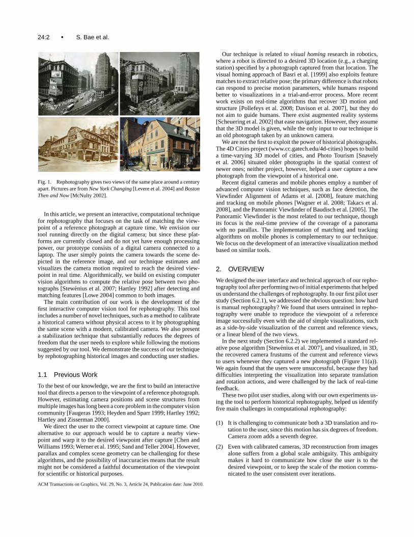
Fig. 2. The first photograph is captured from a location rotated about20 degrees from the user’s best approximation of the desired viewpoint. Thesecond photograph is then captured from the user’s best approximation.

(3) Relative pose algorithms suffer from a degeneracy in the caseof zero motion between the cameras [Torr et al. 1999], whichis exactly our goal. This degeneracy means the estimationbecomes unstable as the user reaches the reference view.

(4) Historical images can appear very different from new pho-tographs because of architectural modifications, different filmresponse, aging, weather, time-of-day, etc. These dramatic dif-ferences can make it challenging for even state-of-the art fea-ture descriptors to find the correspondences needed to computerelative pose.

(5) Finally, historical images are captured with cameras of un-known calibration, for example, focal length and principalpoint. Furthermore, historical architectural photographs wereoften captured with noncentral principal points using viewcameras, to make the vertical lines of building vertical in theimage.

We address these challenges with a combination of user inter-action and algorithms. Our approach has a number of key featureswhich we describe in the rest of this article. The first is our approachto calibration of the unknown camera used to capture the histori-cal image (Section 3), that is, challenge 5. We require the user tocapture two images of the scene with a wide baseline (Figure 2).The user is instructed to capture a first frame and second framewith a roughly 20 degree angle about the main scene subject, withthe second frame as the user’s best eyeballed approximation of thedesired viewpoint. We then reconstruct the scene in 3D and use thisstructure to calibrate the historical camera after asking the user tomanually identify a few correspondences with the historical image(challenge 4). We also use this wide baseline to solve challenge 3 byperforming pose estimation relative to the first frame rather than thereference view, which helps avoid degeneracy. The computed 3Dstructure also helps us to compute a consistent 3D scale across itera-tions (challenge 2). Finally, our calibration method also includes anoptional interactive approach to calibrating a noncentral principalpoint (Section 3.2.1), which asks the user to identify sets of parallellines in the scene.

Another key aspect of our approach is real-time visual guidancethat directs the user towards the desired viewpoint (Section 4).This feedback includes a visualization of the needed 3D translationto the reference view computed by interleaving a slower, robustrelative pose algorithm (Section 4.1) with faster, lightweight updates(Section 4.2). We also use the computed relative pose to performrotation stabilization (Section 4.5); that is, we show the current view

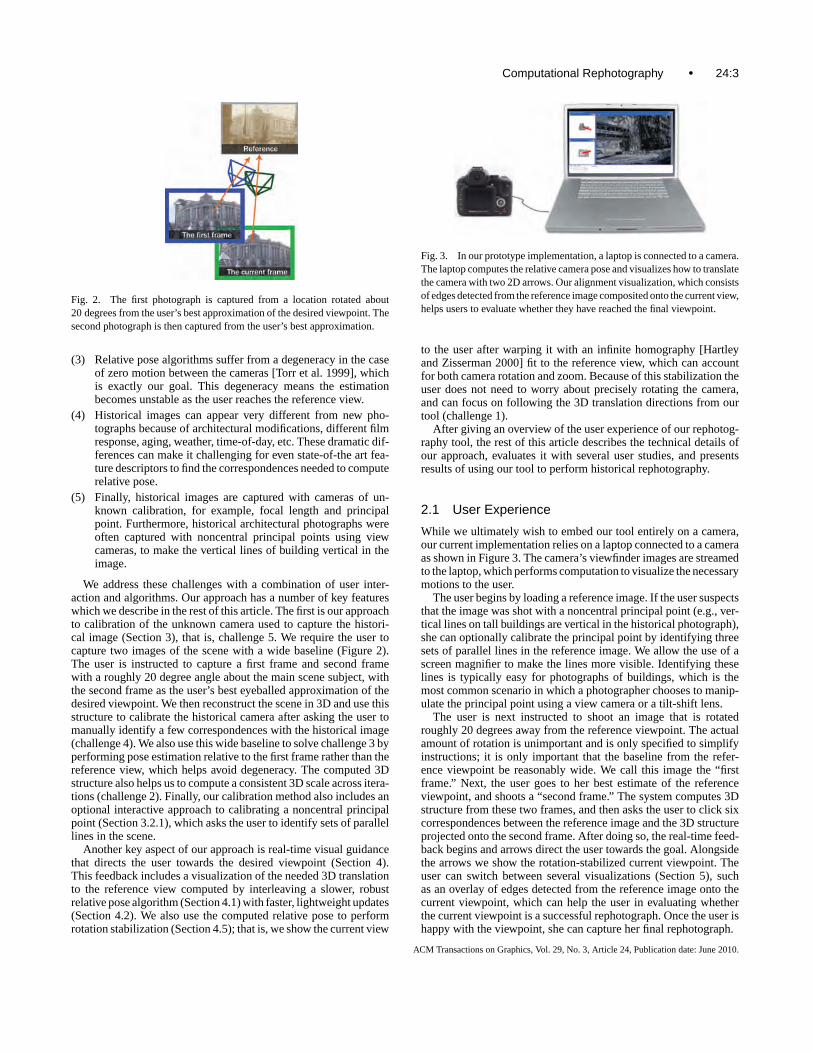
Fig. 3. In our prototype implementation, a laptop is connected to a camera.The laptop computes the relative camera pose and visualizes how to translatethe camera with two 2D arrows. Our alignment visualization, which consistsof edges detected from the reference image composited onto the current view,helps users to evaluate whether they have reached the final viewpoint.

to the user after warping it with an infinite homography [Hartleyand Zisserman 2000] fit to the reference view, which can accountfor both camera rotation and zoom. Because of this stabilization theuser does not need to worry about precisely rotating the camera,and can focus on following the 3D translation directions from ourtool (challenge 1).

After giving an overview of the user experience of our rephotog-raphy tool, the rest of this article describes the technical details ofour approach, evaluates it with several user studies, and presentsresults of using our tool to perform historical rephotography.

2.1 User Experience

While we ultimately wish to embed our tool entirely on a camera,our current implementation relies on a laptop connected to a cameraas shown in Figure 3. The camera’s viewfinder images are streamedto the laptop, which performs computation to visualize the necessarymotions to the user.

The user begins by loading a reference image. If the user suspectsthat the image was shot with a noncentral principal point (e.g., ver-tical lines on tall buildings are vertical in the historical photograph),she can optionally calibrate the principal point by identifying threesets of parallel lines in the reference image. We allow the use of ascreen magnifier to make the lines more visible. Identifying theselines is typically easy for photographs of buildings, which is themost common scenario in which a photographer chooses to manip-ulate the principal point using a view camera or a tilt-shift lens.

The user is next instructed to shoot an image that is rotatedroughly 20 degrees away from the reference viewpoint. The actualamount of rotation is unimportant and is only specified to simplifyinstructions; it is only important that the baseline from the refer-ence viewpoint be reasonably wide. We call this image the “firstframe.” Next, the user goes to her best estimate of the referenceviewpoint, and shoots a “second frame.” The system computes 3Dstructure from these two frames, and then asks the user to click sixcorrespondences between the reference image and the 3D structureprojected onto the second frame. After doing so, the real-time feed-back begins and arrows direct the user towards the goal. Alongsidethe arrows we show the rotation-stabilized current viewpoint. Theuser can switch between several visualizations (Section 5), suchas an overlay of edges detected from the reference image onto thecurrent viewpoint, which can help the user in evaluating whetherthe current viewpoint is a successful rephotograph. Once the user ishappy with the viewpoint, she can capture her final rephotograph.



Fig. 4. Our procedure to calibrate and register the reference camera.

3. CALIBRATION

The first step of our computational rephotography tool is to calibrateboth the intrinsic and extrinsic parameters of the unknown historicalcamera. We do so by performing a sparse 3D reconstruction of thesame scene imaged by the historical camera using two user-capturedimages, and then optimizing the parameters of the unknown camerato minimize projection error of the features manually correspondedby the user. We also optionally allow the user to calibrate a noncen-tral principal point by specifying sets of parallel scene lines in thehistorical image. This process is shown in Figure 4.

3.1 Wide Baseline 3D Reconstruction

The user begins by capturing two images (the first and secondframes) with a wide baseline (Figure 2); a wide baseline improvesthe accuracy and stability of 3D reconstruction. We assume thecurrent camera is calibrated (we use Bouguet’s calibration tool-box [2007]), and then perform structure-from-motion to register thetwo cameras and reconstruct sparse 3D structure. Specifically, weuse the robust pose estimation algorithm described in Section 4.1.In brief, it uses the algorithm of Stewenius et al. [2007] to com-pute relative pose given SIFT [Lowe 2004] correspondences be-tween the two views within a robust sampling loop similar toRANSAC [Fischler and Bolles 1981]. Then, given the projectionmatrices of the two cameras, we reconstruct the 3D coordinates ofeach correspondence using triangulation [Hartley and Zisserman2000]. These 3D points are then projected into the second view, anddisplayed to the user alongside the reference photograph; the useris asked to click 6–8 correspondences. These correspondences areused to register the reference camera in the next step.

3.2 Reference Camera Registration

We next relate the reference image to the reconstructed scene fromthe first two photographs taken by the user, given matches be-tween the reference and the second view. For this, we infer theintrinsic and extrinsic parameters of the reference camera usingLevenberg-Marquardt optimization (specifically, Lourakis’s LMpackage [2004]), minimizing the sum of squared projection errorsof the matched points. We assume zero skew and optimize nine de-grees of freedom: one for focal length, two for the principal point,

Fig. 5. Under perspective projection, parallel lines in space appear to meetat their vanishing point in the image plane. Given the vanishing points ofthree orthogonal directions, the principal point is located at the orthocenterof the triangle with vertices at the vanishing points.

three for rotation, and three for translation. We initialize the rotationmatrix to the identity matrix, the translation matrix to zero, and thefocal length to the focal length of the current camera. We initializethe principal point by analyzing the vanishing points as describedin Section 3.2.1.

Although this initialization is not close to the ground truth, weobserve that the Levenberg-Marquardt algorithm converges to thecorrect answer since we allow only 9 degrees of freedom andthe rotation matrix tends to be close to the identity matrix forrephotography.

3.2.1 Principal Point Estimation. The principal point is theintersection of the optical axis with the image plane. If a shiftmovement is applied to the lens to make the verticals parallel or if theimage is cropped, the principal point is not in the center of the image,and it must be computed. The analysis of vanishing points providesstrong cues for inferring the location of the principal point. Underperspective projection, parallel lines in space appear to meet at asingle point in the image plane; this point is the vanishing point ofthe lines. Given the vanishing points of three orthogonal directions,the principal point is located at the orthocenter of the triangle whosevertices are the vanishing points [Hartley and Zisserman 2000], asshown in Figure 5.

We ask the users to click on three parallel lines in the same di-rection; although two parallel lines are enough for computation, weask for three to improve robustness. We compute the intersectionsof the parallel lines. We locate each vanishing point at the weightedaverage of three intersections. The weight is proportional to the an-gle between two lines [Caprile and Torre 1990], since the locationof the vanishing point becomes less reliable at smaller angles. Wediscard the vanishing point when the sum of the three angles is lessthan 5 degrees.

During Levenberg-Marquardt nonlinear optimization, we initial-ize and constrain the principal point as the orthocenter, given threefinite vanishing points. If we have one finite and two infinite vanish-ing points, we initialize and constrain the principal point as the finitevanishing point. With two finite vanishing points, we constrain theprincipal point to be on the vanishing line that connects the finitevanishing points.

In summary, the result of the preceding methods is a 3D recon-struction of the scene from the first and second frames, as well as acalibration of the reference view and its relative pose from the firstview. This information is then used in the next stage, which guidesthe user to the viewpoint of the reference image.

4. REAL-TIME USER GUIDANCE

Our rephotography tool provides the user with real-time guidancetowards the reference viewpoint. To do so, we compute relative



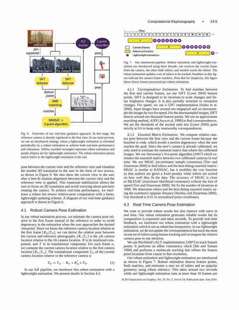
Fig. 6. Overview of our real-time guidance approach. In this stage, thereference camera is already registered to the first view. In our main process,we use an interleaved strategy where a lightweight estimation is refreshedperiodically by a robust estimation to achieve both real-time performanceand robustness. Yellow rounded rectangles represent robust estimation andpurple ellipses are for lightweight estimation. The robust estimation passesmatch inliers to the lightweight estimation at the end.

pose between the current view and the reference view and visualizethe needed 3D translation to the user in the form of two arrows,as shown in Figure 9. We also show the current view to the userafter a best-fit rotation alignment between the current view and thereference view is applied. This rotational stabilization allows theuser to focus on 3D translation and avoid worrying about preciselyrotating the camera. To achieve real-time performance, we inter-leave a robust but slower relative-pose computation with a faster,lightweight updating scheme. A diagram of our real-time guidanceapproach is shown in Figure 6.

4.1 Robust Camera Pose Estimation

In our robust estimation process, we estimate the camera pose rel-ative to the first frame instead of the reference in order to avoiddegeneracy in the estimation when the user approaches the desiredviewpoint. Since we know the reference camera location relative tothe first frame [R10|T10], we can derive the relative pose betweenthe current and reference photographs. [Rij |Tij ] is the j th cameralocation relative to the ith camera location. R is its rotational com-ponent, and T is its translational component. For each frame n,we compute the current camera location relative to the first cameralocation [R1n|T1n]. The translational component T0n of the currentcamera location relative to the reference camera is

T0n = T1n − R1n ∗ R�10 ∗ T10. (1)

In our full pipeline, we interleave this robust estimation with alightweight estimation. We present details in Section 4.2.

Fig. 7. Our interleaved pipeline. Robust estimation and lightweight esti-mation are interleaved using three threads: one receives the current framefrom the camera, the other finds inliers, and another tracks the inliers. Therobust estimation updates a set of inliers to be tracked. Numbers in this fig-ure indicate the camera frame numbers. Note that for simplicity, this figureshows fewer frames processed per robust estimation.

4.1.1 Correspondence Estimation. To find matches betweenthe first and current frames, we use SIFT [Lowe 2004] featurepoints. SIFT is designed to be invariant to scale changes and lin-ear brightness changes. It is also partially invariant to viewpointchanges. For speed, we use a GPU implementation [Sinha et al.2006]. Input images have around one megapixel and we downsam-ple the images by two for speed. For the downsampled images, SIFTdetects around one thousand feature points. We use an approximatesearching method, ANN [Arya et al. 1998] to find correspondences.We set the threshold of the second ratio test [Lowe 2004] quitestrictly at 0.6 to keep only trustworthy correspondences.

4.1.2 Essential Matrix Estimation. We compute relative cam-era pose between the first view and the current frame because thebaseline is wide, which avoids a motion degeneracy when the userreaches the goal. Since the user’s camera is already calibrated, weonly need to estimate the essential matrix that relates the calibratedimages. We use Stewenius’s five-point algorithm [2007] which es-timates the essential matrix between two calibrated cameras in realtime. We run MSAC (m-estimator sample consensus) [Torr andZisserman 2000] to find inliers and the best-fitting essential matrix.MSAC is similar to RANSAC, but it modifies the cost functionso that outliers are given a fixed penalty while inliers are scoredon how well they fit the data. The accuracy of MSAC is closeto MLESAC (maximum likelihood consensus) without the loss ofspeed [Torr and Zisserman 2000]. We fix the number of iterations at1000. We determine inliers and the best-fitting essential matrix us-ing the symmetric epipolar distance [Hartley and Zisserman 2000].Our threshold is 0.01 in normalized point coordinates.

4.2 Real-Time Camera Pose Estimation

We want to provide robust results but also interact with users inreal time. Our robust estimation generates reliable results but itscomputation is expensive and takes seconds. To provide real-timefeedback, we interleave our robust estimation with a lightweightestimation which is not as robust but inexpensive. In our lightweightestimation, we do not update the correspondences but track the mostrecent set of inliers using feature tracking and recompute the relativecamera pose in one iteration.

We use Birchfield’s KLT implementation [2007] to track featurepoints. It performs an affine consistency check [Shi and Tomasi1994] and performs a multiscale tracking that refines the featurepoint locations from coarse to fine resolution.

Our robust estimation and lightweight estimation are interleavedas shown in Figure 7. Robust estimation detects feature points,finds matches, and estimates a new set of inliers and an epipolargeometry using robust statistics. This takes around two secondswhile our lightweight estimation runs at more than 10 frames per



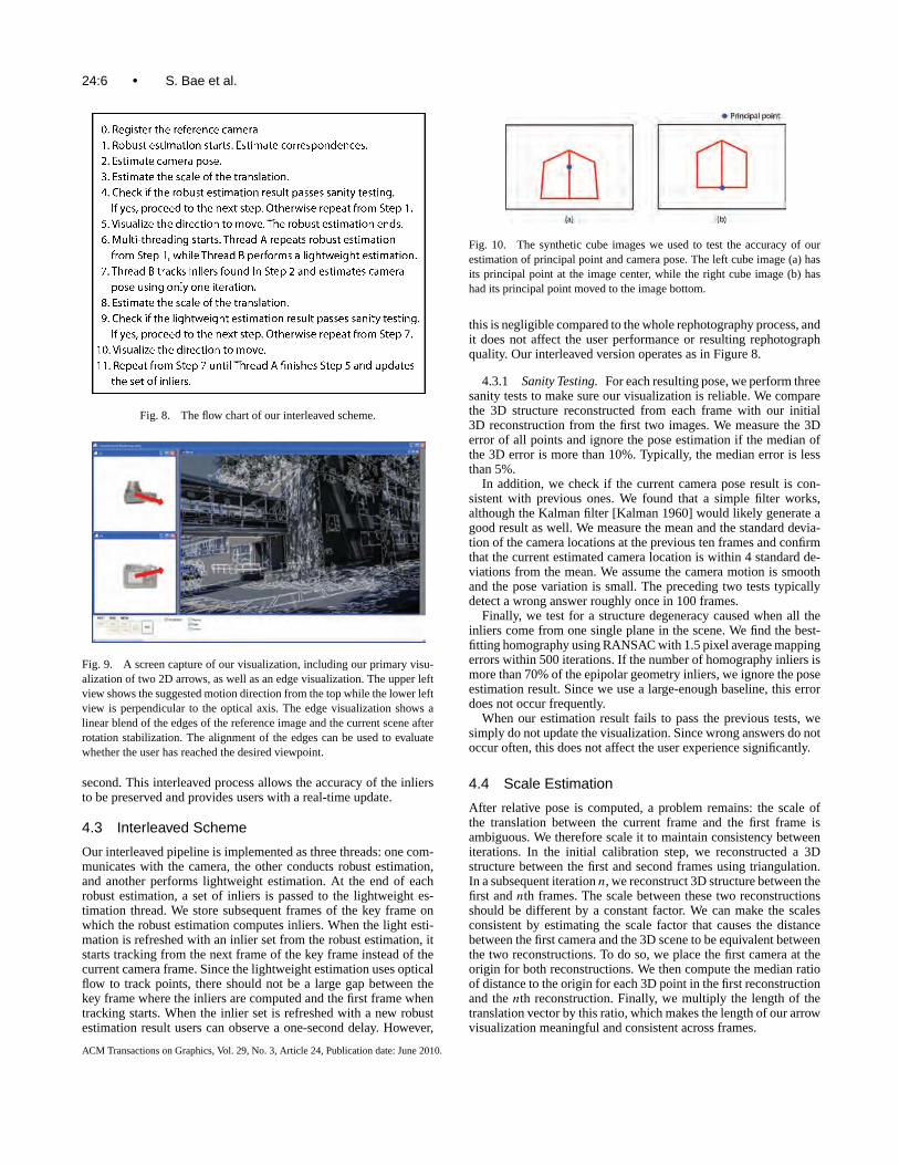
Fig. 8. The flow chart of our interleaved scheme.

Fig. 9. A screen capture of our visualization, including our primary visu-alization of two 2D arrows, as well as an edge visualization. The upper leftview shows the suggested motion direction from the top while the lower leftview is perpendicular to the optical axis. The edge visualization shows alinear blend of the edges of the reference image and the current scene afterrotation stabilization. The alignment of the edges can be used to evaluatewhether the user has reached the desired viewpoint.

second. This interleaved process allows the accuracy of the inliersto be preserved and provides users with a real-time update.

4.3 Interleaved Scheme

Our interleaved pipeline is implemented as three threads: one com-municates with the camera, the other conducts robust estimation,and another performs lightweight estimation. At the end of eachrobust estimation, a set of inliers is passed to the lightweight es-timation thread. We store subsequent frames of the key frame onwhich the robust estimation computes inliers. When the light esti-mation is refreshed with an inlier set from the robust estimation, itstarts tracking from the next frame of the key frame instead of thecurrent camera frame. Since the lightweight estimation uses opticalflow to track points, there should not be a large gap between thekey frame where the inliers are computed and the first frame whentracking starts. When the inlier set is refreshed with a new robustestimation result users can observe a one-second delay. However,

Fig. 10. The synthetic cube images we used to test the accuracy of ourestimation of principal point and camera pose. The left cube image (a) hasits principal point at the image center, while the right cube image (b) hashad its principal point moved to the image bottom.

this is negligible compared to the whole rephotography process, andit does not affect the user performance or resulting rephotographquality. Our interleaved version operates as in Figure 8.

4.3.1 Sanity Testing. For each resulting pose, we perform threesanity tests to make sure our visualization is reliable. We comparethe 3D structure reconstructed from each frame with our initial3D reconstruction from the first two images. We measure the 3Derror of all points and ignore the pose estimation if the median ofthe 3D error is more than 10%. Typically, the median error is lessthan 5%.

In addition, we check if the current camera pose result is con-sistent with previous ones. We found that a simple filter works,although the Kalman filter [Kalman 1960] would likely generate agood result as well. We measure the mean and the standard devia-tion of the camera locations at the previous ten frames and confirmthat the current estimated camera location is within 4 standard de-viations from the mean. We assume the camera motion is smoothand the pose variation is small. The preceding two tests typicallydetect a wrong answer roughly once in 100 frames.

Finally, we test for a structure degeneracy caused when all theinliers come from one single plane in the scene. We find the best-fitting homography using RANSAC with 1.5 pixel average mappingerrors within 500 iterations. If the number of homography inliers ismore than 70% of the epipolar geometry inliers, we ignore the poseestimation result. Since we use a large-enough baseline, this errordoes not occur frequently.

When our estimation result fails to pass the previous tests, wesimply do not update the visualization. Since wrong answers do notoccur often, this does not affect the user experience significantly.

4.4 Scale Estimation

After relative pose is computed, a problem remains: the scale ofthe translation between the current frame and the first frame isambiguous. We therefore scale it to maintain consistency betweeniterations. In the initial calibration step, we reconstructed a 3Dstructure between the first and second frames using triangulation.In a subsequent iteration n, we reconstruct 3D structure between thefirst and nth frames. The scale between these two reconstructionsshould be different by a constant factor. We can make the scalesconsistent by estimating the scale factor that causes the distancebetween the first camera and the 3D scene to be equivalent betweenthe two reconstructions. To do so, we place the first camera at theorigin for both reconstructions. We then compute the median ratioof distance to the origin for each 3D point in the first reconstructionand the nth reconstruction. Finally, we multiply the length of thetranslation vector by this ratio, which makes the length of our arrowvisualization meaningful and consistent across frames.



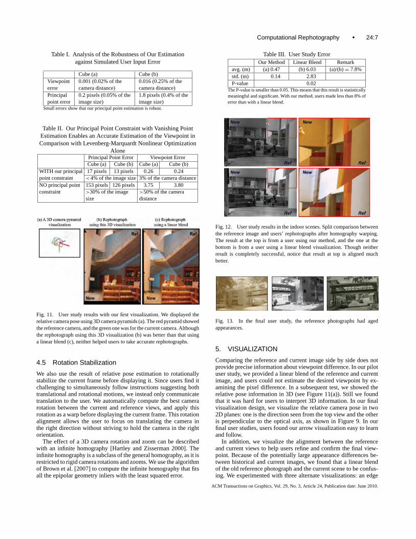
Table I. Analysis of the Robustness of Our Estimationagainst Simulated User Input Error

Cube (a) Cube (b)Viewpoint 0.001 (0.02% of the 0.016 (0.25% of theerror camera distance) camera distance)Principal 0.2 pixels (0.05% of the 1.8 pixels (0.4% of thepoint error image size) image size)

Small errors show that our principal point estimation is robust.

Table II. Our Principal Point Constraint with Vanishing PointEstimation Enables an Accurate Estimation of the Viewpoint inComparison with Levenberg-Marquardt Nonlinear Optimization

AlonePrincipal Point Error Viewpoint ErrorCube (a) Cube (b) Cube (a) Cube (b)

WITH our principal 17 pixels 13 pixels 0.26 0.24point constraint <4% of the image size 3% of the camera distanceNO principal point 153 pixels 126 pixels 3.75 3.80constraint >30% of the image >50% of the camera

size distance

Fig. 11. User study results with our first visualization. We displayed therelative camera pose using 3D camera pyramids (a). The red pyramid showedthe reference camera, and the green one was for the current camera. Althoughthe rephotograph using this 3D visualization (b) was better than that usinga linear blend (c), neither helped users to take accurate rephotographs.

4.5 Rotation Stabilization

We also use the result of relative pose estimation to rotationallystabilize the current frame before displaying it. Since users find itchallenging to simultaneously follow instructions suggesting bothtranslational and rotational motions, we instead only communicatetranslation to the user. We automatically compute the best camerarotation between the current and reference views, and apply thisrotation as a warp before displaying the current frame. This rotationalignment allows the user to focus on translating the camera inthe right direction without striving to hold the camera in the rightorientation.

The effect of a 3D camera rotation and zoom can be describedwith an infinite homography [Hartley and Zisserman 2000]. Theinfinite homography is a subclass of the general homography, as it isrestricted to rigid camera rotations and zooms. We use the algorithmof Brown et al. [2007] to compute the infinite homography that fitsall the epipolar geometry inliers with the least squared error.

Table III. User Study ErrorOur Method Linear Blend Remark

avg. (m) (a) 0.47 (b) 6.03 (a)/(b) = 7.8%std. (m) 0.14 2.83P-value 0.02

The P-value is smaller than 0.05. This means that this result is statisticallymeaningful and significant. With our method, users made less than 8% oferror than with a linear blend.

Fig. 12. User study results in the indoor scenes. Split comparison betweenthe reference image and users’ rephotographs after homography warping.The result at the top is from a user using our method, and the one at thebottom is from a user using a linear blend visualization. Though neitherresult is completely successful, notice that result at top is aligned muchbetter.

Fig. 13. In the final user study, the reference photographs had agedappearances.

5. VISUALIZATION

Comparing the reference and current image side by side does notprovide precise information about viewpoint difference. In our pilotuser study, we provided a linear blend of the reference and currentimage, and users could not estimate the desired viewpoint by ex-amining the pixel difference. In a subsequent test, we showed therelative pose information in 3D (see Figure 11(a)). Still we foundthat it was hard for users to interpret 3D information. In our finalvisualization design, we visualize the relative camera pose in two2D planes: one is the direction seen from the top view and the otheris perpendicular to the optical axis, as shown in Figure 9. In ourfinal user studies, users found our arrow visualization easy to learnand follow.

In addition, we visualize the alignment between the referenceand current views to help users refine and confirm the final view-point. Because of the potentially large appearance differences be-tween historical and current images, we found that a linear blendof the old reference photograph and the current scene to be confus-ing. We experimented with three alternate visualizations: an edge



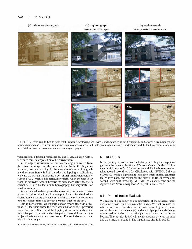
Fig. 14. User study results. Left to right: (a) the reference photograph and users’ rephotographs using our technique (b) and a naıve visualization (c) afterhomography warping. The second row shows a split comparison between the reference image and users’ rephotographs, and the third row shows a zoomed-ininset. With our method, users took more accurate rephotographs.

visualization, a flipping visualization, and a visualization with areference camera projected onto the current frame.

In the edge visualization, we overlay the edges extracted fromthe reference image over the current frame. In the flipping visu-alization, users can quickly flip between the reference photographand the current frame. In both the edge and flipping visualizations,we warp the current frame using a best-fitting infinite homography(Section 4.5), which is not particularly useful when the user is farfrom the desired viewpoint because the current and reference viewscannot be related by the infinite homography, but very useful forsmall translations.

As the translational component becomes zero, the rotational com-ponent is well resolved by a homography. Finally, for the third vi-sualization we simply project a 3D model of the reference cameraonto the current frame, to provide a visual target for the user.

During user studies, we let users choose among three visualiza-tions. All the users chose the edge visualization as their preferredvisual feedback. Users used the flipping visualization only at thefinal viewpoint to confirm the viewpoint. Users did not find theprojected reference camera very useful. Figure 9 shows our finalvisualization design.

6. RESULTS

In our prototype, we estimate relative pose using the output weget from the camera viewfinder. We use a Canon 1D Mark III liveview, which outputs 5–10 frames per second. Each robust estimationtakes about 2 seconds on a 2.4 GHz laptop with NVIDIA GeForce8600M GT, while a lightweight estimation tracks inliers, estimatesthe relative pose, and visualizes the arrows at 10–20 frames persecond. With multithreading, GPU-SIFT takes one second and theApproximate Nearest Neighbor (ANN) takes one second.

6.1 Preregistration Evaluation

We analyze the accuracy of our estimation of the principal pointand camera pose using two synthetic images. We first evaluate therobustness of our estimation to user input error. Figure 10 showsour synthetic test cases: cube (a) has its principal point at the imagecenter, and cube (b) has its principal point moved to the imagebottom. The cube size is 3×3×3, and the distance between the cubeand the camera is around 6. The input image size is 512×340.



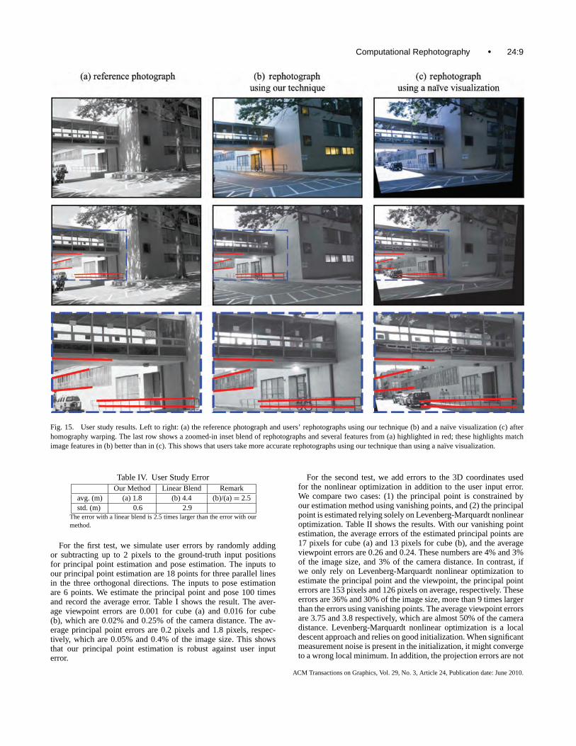
Fig. 15. User study results. Left to right: (a) the reference photograph and users’ rephotographs using our technique (b) and a naıve visualization (c) afterhomography warping. The last row shows a zoomed-in inset blend of rephotographs and several features from (a) highlighted in red; these highlights matchimage features in (b) better than in (c). This shows that users take more accurate rephotographs using our technique than using a naıve visualization.

Table IV. User Study ErrorOur Method Linear Blend Remark

avg. (m) (a) 1.8 (b) 4.4 (b)/(a) = 2.5std. (m) 0.6 2.9

The error with a linear blend is 2.5 times larger than the error with ourmethod.

For the first test, we simulate user errors by randomly addingor subtracting up to 2 pixels to the ground-truth input positionsfor principal point estimation and pose estimation. The inputs toour principal point estimation are 18 points for three parallel linesin the three orthogonal directions. The inputs to pose estimationare 6 points. We estimate the principal point and pose 100 timesand record the average error. Table I shows the result. The aver-age viewpoint errors are 0.001 for cube (a) and 0.016 for cube(b), which are 0.02% and 0.25% of the camera distance. The av-erage principal point errors are 0.2 pixels and 1.8 pixels, respec-tively, which are 0.05% and 0.4% of the image size. This showsthat our principal point estimation is robust against user inputerror.

For the second test, we add errors to the 3D coordinates usedfor the nonlinear optimization in addition to the user input error.We compare two cases: (1) the principal point is constrained byour estimation method using vanishing points, and (2) the principalpoint is estimated relying solely on Levenberg-Marquardt nonlinearoptimization. Table II shows the results. With our vanishing pointestimation, the average errors of the estimated principal points are17 pixels for cube (a) and 13 pixels for cube (b), and the averageviewpoint errors are 0.26 and 0.24. These numbers are 4% and 3%of the image size, and 3% of the camera distance. In contrast, ifwe only rely on Levenberg-Marquardt nonlinear optimization toestimate the principal point and the viewpoint, the principal pointerrors are 153 pixels and 126 pixels on average, respectively. Theseerrors are 36% and 30% of the image size, more than 9 times largerthan the errors using vanishing points. The average viewpoint errorsare 3.75 and 3.8 respectively, which are almost 50% of the cameradistance. Levenberg-Marquardt nonlinear optimization is a localdescent approach and relies on good initialization. When significantmeasurement noise is present in the initialization, it might convergeto a wrong local minimum. In addition, the projection errors are not


24:10 • S. Bae et al.

Fig. 16. Results. Left to right: the reference images, our rephotograph results, and professional manual rephotographs without our method.

discriminative enough to determine the viewpoint and the principalpoint at the same time. There exist ambiguities between changingthe principal point and moving the camera. This is reduced by thevanishing point method.

Finally we analyze the effect of varying the focal length whilechanging the camera distance. As a result, the size of the projectedcube stays the same, but camera rotation and principal point modi-fication become harder to disambiguate. The focal lengths used are400, 600, 800, and 1000. 400 is equivalent to 20mm, and 1000 isequivalent to 50mm for a 35mm film. The errors increase as the focallength and the camera distance increase. The principal point errorsare 13, 27, 45, and 66 pixels respectively, which are 3%, 6%, 11%,and 15% of the image size. The viewpoint errors are 0.4, 0.6, 1.15,and 1.86, which are 5%, 5%, 7%, and 9% of the camera distance.The more we zoom, the more ambiguous the estimation becomes.This is related to the fact that the projection error is less discrimina-tive for a photograph taken by a telephoto lens, because the effectof a 3D rotation and that of a 2D translation become similar.

6.2 User Interface Evaluation

We performed multiple pilot user studies before finalizing the de-sign of our user interface. The studies included eight females and

eight males with ages ranging from 22–35. Only one of them partic-ipated in multiple studies. We recruited the participants via personalcontacts; eight of them had computer science backgrounds, whilethe other eight did not.

6.2.1 First Pilot User Study. In our first pilot user study, wewanted to test whether humans would be able to estimate the view-point differences by simply comparing two photographs.

Procedure. We asked users to estimate the viewpoint of a ref-erence photograph by comparing it with the output of the cameraviewfinder, while they moved the camera. We provided two userswith three different visualization techniques: the reference and cur-rent image side by side, a linear blend of the reference and currentimage, and a color-coded linear blend of the reference in red andcurrent image in blue. We asked the users questions upon comple-tion of the task.

Results and conclusions. Comparing the reference and currentimage side by side did not seem to provide information aboutviewpoint differences; both the user’s final rephotographs werepoor. Although users preferred the linear blend among three vi-sualization, the users could still not estimate the desired view-point by examining parallax. This leads to our first visualizationdesign.



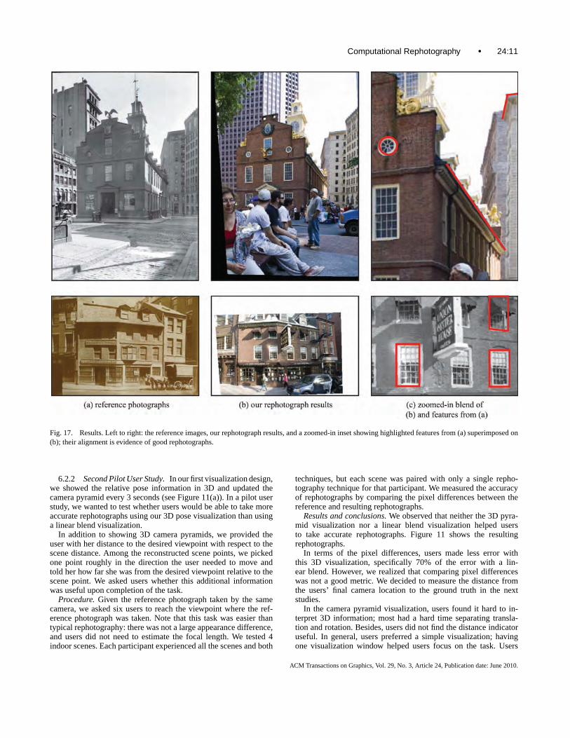
Fig. 17. Results. Left to right: the reference images, our rephotograph results, and a zoomed-in inset showing highlighted features from (a) superimposed on(b); their alignment is evidence of good rephotographs.

6.2.2 Second Pilot User Study. In our first visualization design,we showed the relative pose information in 3D and updated thecamera pyramid every 3 seconds (see Figure 11(a)). In a pilot userstudy, we wanted to test whether users would be able to take moreaccurate rephotographs using our 3D pose visualization than usinga linear blend visualization.

In addition to showing 3D camera pyramids, we provided theuser with her distance to the desired viewpoint with respect to thescene distance. Among the reconstructed scene points, we pickedone point roughly in the direction the user needed to move andtold her how far she was from the desired viewpoint relative to thescene point. We asked users whether this additional informationwas useful upon completion of the task.

Procedure. Given the reference photograph taken by the samecamera, we asked six users to reach the viewpoint where the ref-erence photograph was taken. Note that this task was easier thantypical rephotography: there was not a large appearance difference,and users did not need to estimate the focal length. We tested 4indoor scenes. Each participant experienced all the scenes and both

techniques, but each scene was paired with only a single repho-tography technique for that participant. We measured the accuracyof rephotographs by comparing the pixel differences between thereference and resulting rephotographs.

Results and conclusions. We observed that neither the 3D pyra-mid visualization nor a linear blend visualization helped usersto take accurate rephotographs. Figure 11 shows the resultingrephotographs.

In terms of the pixel differences, users made less error withthis 3D visualization, specifically 70% of the error with a lin-ear blend. However, we realized that comparing pixel differenceswas not a good metric. We decided to measure the distance fromthe users’ final camera location to the ground truth in the nextstudies.

In the camera pyramid visualization, users found it hard to in-terpret 3D information; most had a hard time separating transla-tion and rotation. Besides, users did not find the distance indicatoruseful. In general, users preferred a simple visualization; havingone visualization window helped users focus on the task. Users


24:12 • S. Bae et al.

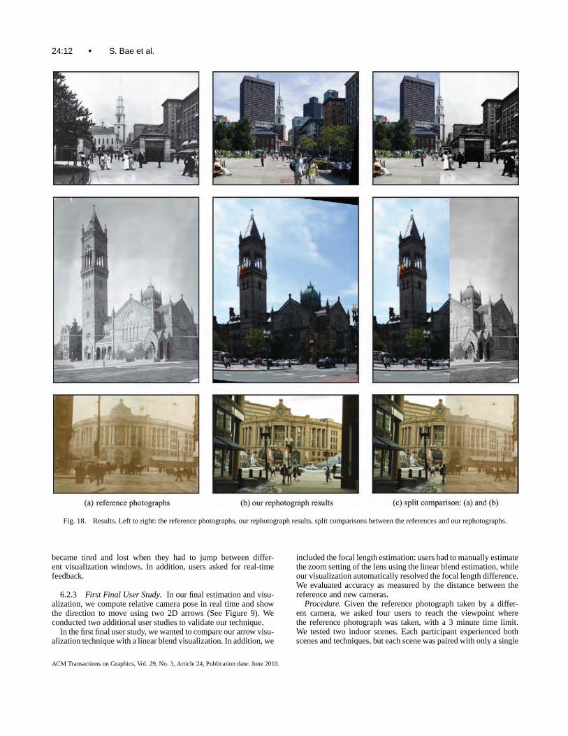
Fig. 18. Results. Left to right: the reference photographs, our rephotograph results, split comparisons between the references and our rephotographs.

became tired and lost when they had to jump between differ-ent visualization windows. In addition, users asked for real-timefeedback.

6.2.3 First Final User Study. In our final estimation and visu-alization, we compute relative camera pose in real time and showthe direction to move using two 2D arrows (See Figure 9). Weconducted two additional user studies to validate our technique.

In the first final user study, we wanted to compare our arrow visu-alization technique with a linear blend visualization. In addition, we

included the focal length estimation: users had to manually estimatethe zoom setting of the lens using the linear blend estimation, whileour visualization automatically resolved the focal length difference.We evaluated accuracy as measured by the distance between thereference and new cameras.

Procedure. Given the reference photograph taken by a differ-ent camera, we asked four users to reach the viewpoint wherethe reference photograph was taken, with a 3 minute time limit.We tested two indoor scenes. Each participant experienced bothscenes and techniques, but each scene was paired with only a single



Fig. 19. Results with style transfer. Left to right: the reference photographs, our rephotograph results, and our rephotographs with styles transferred from thereference photographs.

rephotography technique for that participant. We marked the refer-ence camera location on the map and measured the distance fromthe users’ final camera location to the ground truth. We did not askusers to choose the first and second viewpoints; they were fixedamong all the users.

Results and conclusions. Table III shows the average distancebetween the ground truth and the final locations where four userstook the rephotographs for two test cases. The error with our methodwas less than 8% of the error with a linear blend. Users found that our2D arrows were easy to learn and follow. Figure 12 compares tworephotograph results using both techniques. In every test case, users

took more accurate rephotographs with our arrow visualization thanwith a linear blend visualization.

6.2.4 Second Final User Study. In our final user study, wewanted to test our user interaction schemes including providinga wide-baseline, clicking on matches, and comparing two pho-tographs with large appearance differences. We compared the ac-curacies of the resulting rephotographs using our technique againstthose with a naıve visualization. In particular, we sought to comparethe accuracy of the viewpoint localization.

Procedure. We compared our technique with a naıve visualiza-tion and used reference images for which the ground-truth location


24:14 • S. Bae et al.

is known. To make the scenario more realistic, we simulated anaged appearance on the reference photographs that we captured: wetransferred the tonal aspects from old photograph samples to thereference photographs [Bae et al. 2006], as shown in Figure 13. Asa result, the reference photographs had large appearance differencesfrom current photographs. We asked six users to reach the view-point where the reference photograph was taken within 10 mins.We tested three outdoor scenes. Each participant experienced allthe scenes and both techniques, but each scene paired with only asingle technique for that participant.

For both methods, all users started from the same initial location.With our technique, we only fixed the first viewpoint (as the initiallocation), and asked users to choose the second viewpoint. In ad-dition, users provided correspondences between the reference andthe second frame by clicking six matches. In the naıve visualizationmethod, we showed both linear blend and side-by-side visual-izations of the reference and current frame, since a linear blendsuffered from large appearance differences between the referenceand current photographs. Again, users had to manually estimatethe zoom setting of the lens using the naıve visualization, while ourvisualization automatically resolved the focal length difference. Be-fore each user study, we provided users with a quick tutorial of bothmethods.

Results and conclusions. In every test case, users took moreaccurate rephotographs with our arrow visualization than with thenaıve visualizations. Figures 14 and 15 compare the rephotographstaken with our technique and those using a naıve visualization.The remaining parallax in the rephotograph results using a naıvevisualization is quite large, while our technique allowed users tominimize parallax.

Table IV shows the average distance between the ground truthand the final locations where six users took the rephotographs forthree test cases. The average error with our method is 40% of theaverage error with a linear blend. The distance difference becamesmaller than the indoor cases. In the indoor scenes, the parallax wassubtle, but in the outdoor scenes, users could notice some importantcues such as whether buildings were occluded or not. Still manypeople could not figure out how to move the camera to resolvethe parallax. With a naıve blend, users had to estimate the locationand focal length of the reference camera by themselves. With ourmethod, users needed only to follow our arrow visualization whileour technique automatically estimated the location and focal lengthof the reference camera.

6.3 Results on Historical Photographs

Figures 16, 17, 18, and 19 show our rephotograph results of histor-ical photographs taken by unknown cameras. It usually took 15–30minutes to reach the desired viewpoint. This task required moreextensive time because we often had to walk 50–100m with a lap-top and tripod, and cross busy roads. In Figure 19, we apply styletransfer from the reference to the rephotographs [Bae et al. 2006].By matching the tonal aspects, it becomes even more evident whichscene elements are preserved and which have changed across time.Faithful rephotographs reveal the changes of roofs, windows, andthe overall neighborhood.

6.4 Discussion

The bulk of the laptop currently limits portability and we hope thatopen-platform digital cameras with additional processing powerwill enable rephotography directly from the camera.

Our relative pose estimation works best when there is sufficientparallax between the images. When nearing the viewpoint, the user

typically relies more on the alignment blend, which can limit finalprecision. Our technique requires a reasonable number of featurepoints (around 20), and can suffer in scenes with little texture.The scene must present enough 3D structure to make viewpointestimation well-posed. If the scene is mostly planar, a homog-raphy can match any pair of views and the viewpoint cannot beinferred.

In addition, the resulting rephotograph’s precision depends onthe user’s tolerance for error. For example, users typically focuson landmarks in the center of the image, and may not notice thatfeatures towards the periphery are not well-aligned. If the user onlychecks alignment in the center, parallax towards the periphery maynot be resolved, as in Figures 15 and 17.

We share a number of limitations with traditional rephotography:if the desired viewpoint is not available or the scene is occluded andcannot be seen at the desired viewpoint, rephotography is impossi-ble. Nevertheless, our technique can still help users realize that theviewpoint is no longer available.

Audio feedback is a natural extension to our visualization thatwe hope to explore in the future.

7. CONCLUSIONS

In this article we described a real-time pose estimation and visu-alization technique for guiding a user while performing rephotog-raphy. Our method includes an approach to calibrating the histor-ical camera by taking several photographs of the same scene, awide-baseline reconstruction that avoids relative pose estimationdegeneracy when the user reaches the desired target, and a visu-alization technique that guides the user with two 2D arrows and arotationally-stabilized current view.

We believe that our work points towards an exciting longer-termdirection: embedding more computation in cameras to support morecomplex interaction at capture time than is offered by current com-modity hardware. While our prototype requires a laptop connectedto a camera, we hope that more open camera platforms are devel-oped in the future that allow more experimentation in designingnovel user interfaces that can run on the camera.

ACKNOWLEDGMENTS

We thank the MIT Computer Graphics Group, Adobe’s AdvancedTechnology Labs, the anonymous reviewers and prereviewers, andNoah Snavely for their comments. This work was supported bygrants from Quanta, Shell, and Adobe. Thanks to the publishers ofthe rephotography books for their images.

REFERENCES

ADAMS, A., GELFAND, N., AND PULLI, K. 2008. Viewfinder alignment.Comput. Graph. Forum 27, 2, 597–606.

ARYA, S., MOUNT, D. M., NETANYAHU, N. S., SILVERMAN, R., AND WU, A.1998. An optimal algorithm for approximate nearest neighbor searchingfixed dimensions. J. ACM 45, 6, 891–923.

BAE, S., PARIS, S., AND DURAND, F. 2006. Two-Scale tone managementfor photographic look. ACM Trans. Graph. 25, 3, 637–645.

BASRI, R., RIVLIN, E., AND SHIMSHONI, I. 1999. Visual homing: Surfingon the epipoles. Int. J. Comput. Vis. 33, 2, 117–137.

BAUDISCH, P., TAN, D., STEEDLY, D., RUDOLPH, E., UYTTENDAELE, M., PAL, C.,AND SZELISKI, R. 2005. Panoramic viewfinder: Providing a real-timepreview to help users avoid flaws in panoramic pictures. In Proceedings of



the 17th Australia Conference on Computer-Human Interaction (OZCHI).1–10.

BIRCHFIELD, S. 2007. KLT: An implementation of the kanade-lucas-tomasi feature tracker. http://www.ces.clemson.edu/stb/klt/.

BOUGUET, J.-Y. 2007. Camera calibration toolbox for matlab.http://www.vision.caltech.edu/bouguetj/calib doc/.

BROWN, M., HARTLEY, R., AND NISTER, D. 2007. Minimal solutions forpanoramic stitching. Comput. Vis. Pattern Recog., 1–8.

CAPRILE, B. AND TORRE, V. 1990. Using vanishing points for cameracalibration. Int. J. Comput. Vis. 4, 2, 127–139.

CHEN, S. E. AND WILLIAMS, L. 1993. View interpolation for imagesynthesis. In SIGGRAPH’93. ACM, New York, 279–288.

DAVISON, A., REID, I., MOLTON, N., AND STASSE, O. 2007. Monoslam: Real-time single camera slam. IEEE Trans. Pattern Anal. Mach. Intel. 29, 6,1052–1067.

FAUGERAS, O. 1993. Three-Dimensional Computer Vision: A GeometricViewpoint. MIT Press, Cambridge, MA.

FISCHLER, M. A. AND BOLLES, R. C. 1981. Random sample consensus:A paradigm for model fitting with applications to image analysis andautomated cartography. Comm. ACM 24. 6, 381–395.

GORE, A. 2006. An Inconvenient Truth. Paramount Classics.HALL, F. C. 2002. Photo point monitoring handbook. Tech. rep. PNW-GTR-

526, USDA Forest Service.HARTLEY, R. I. 1992. Estimation of relative camera positions for uncali-

brated cameras. In Proceedings of the European Conference on ComputerVision (ECCV). 579–587.

HARTLEY, R. I. AND ZISSERMAN, A. 2000. Multiple View Geometry inComputer Vision. Cambridge University Press.

HEYDEN, A. AND SPARR, G. 1999. Reconstruction from calibratedcameras—A new proof of the Kruppa-Demazure theorem. J. Math. Imag.Vis. 10, 2, 123–142.

KALMAN, R. E. 1960. A new approach to linear filtering and predictionproblems. Trans. ASME – J. Basic Engin. 82, Series D, 35–45.

KANG, S. B. AND SHUM, H.-Y. 2002. A review of image-based renderingtechniques. In Proceedings of the IEEE/SPIE Visual Communicationsand Image Processing Conference. 2–13.

KLETT, M., MANCHESTER, E., VERBURG, J., BUSHAW, G., AND DINGUS, R.1990. Second View: The Rephotographic Survey Project. University ofNew Mexico Press.

LEVERE, D., YOCHELSON, B., AND GOLDBERGER, P. 2004. New YorkChanging: Revisiting Berenice Abbott’s New York. Princeton Architec-tural Press.

LOURAKIS, M.. 2004. levmar: Levenberg-Marquardt nonlinear leastsquares algorithms in C/C++. http://www.ics.forth.gr/∼lourakis/levmar/.

LOWE, D. 2004. Distinctive image features from scale-invariant key-points. Int. J. Comput. Vis. 60, 2, 91–110.

MCNULTY, E. 2002. Boston Then and Now. Thunder Bay Press.POLLEFEYS, M., NISTER, D., FRAHM, J. M., AKBARZADEH, A., MORDO-

HAI, P., CLIPP, B., ENGELS, C., GALLUP, D., KIM, S. J., MERRELL, P.,SALMI, C., SINHA, S., TALTON, B., WANG, L., YANG, Q., STEWENIUS, H.,YANG, R., WELCH, G., AND TOWLES, H. 2008. Detailed real-time ur-ban 3D reconstruction from video. Int. J. Comput. Vis. 78, 2-3, 143–167.

SAND, P. AND TELLER, S. 2004. Video matching. ACM Trans.Graph. 23, 3, 592–599.

SCHEUERING, M., REZK-SALAMA, C., BARFUFL, H., SCHNEIDER, A., AND

GREINER, G. 2002. Augmented reality based on fast deformable 2D-3D registration for image-guided surgery. In Proceedings of the SPIE(Medical Imaging: Visualization, Image-Guided Procedures, and Dis-play). Vol. 4681. 436–445.

SHI, J. AND TOMASI, C. 1994. Good features to track. In Proceedingsof the IEEE Conference on Computer Vision and Pattern Recognition(CVPR). 593–600.

SINHA, S. N., FRAHM, J.-M., POLLEFEYS, M., AND GENC, Y. 2006. GPU-based video feature tracking and matching. In Proceedings of theWorkshop on Edge Computing Using New Commodity Architectures(EDGE).

SNAVELY, N., SEITZ, S. M., AND SZELISKI, R. 2006. Photo tourism: Ex-ploring photo collections in 3D. ACM Trans. Graph. 25, 3, 835–846.

STEWENIUS, H., ENGELS, C., AND NISTER, D. 2007. An efficient min-imal solution for infinitesimal camera motion. In Proceedings ofthe Conference on Computer Vision and Pattern Recognition (CVPR).1–8.

TAKACS, G., CHANDRASEKHAR, V., GELFAND, N., XIONG, Y., CHEN, W.-C.,BISMPIGIANNIS, T., GRZESZCZUK, R., PULLI, K., AND GIROD, B. 2008.Outdoors augmented reality on mobile phone using loxel-based visualfeature organization. In Proceedings of the ACM International Conferenceon Multimedia Information Retrieval. 427–434.

TORR, P., FITZGIBBON, A., AND ZISSERMAN, A. 1999. The problem ofdegeneracy in structure and motion recovery from uncalibrated images.Int. J. Computer Vis. 32, 1, 27–44.

TORR, P. H. S. AND ZISSERMAN, A. 2000. MLESAC: A new robustestimator with application to estimating image geometry. Comput. Vis.Image Understand. 78, 1, 138–156.

WAGNER, D., REITMAYR, G., MULLONI, A., DRUMMOND, T., AND

SCHMALSTIEG, D. 2008. Pose tracking from natural features on mobilephones. In Proceedings of the IEEE/ACM International Symposium onMixed and Augmented Reality. 125–134.

WERNER, T., HERSCH, R. D., AND HLAVAC, V. 1995. Rendering real-worldobjects using view interpolation. In Proceedings of the InternationalConference on Computer Vision (ICCV). 957–962.

Received October 2009; rivised February 2010; accepted April 2010


Documents

Computational rephotography - Agarwala · Additional Key Words and Phrases: Computational photography, pose estimation, rephotography ACM Reference Format: ... Computational Rephotography