Embed Size (px)
Citation preview

Development about composite homogenization in static
and in dynamic - application to UD composite materials
Jianhui Yang
Supervisor: Patrick Rozycki
l’Institut de Recherche en Genie Civil et Mecanique
Ecole Centrale de Nantes
A thesis submitted for the degree of
Erasmus Mundus Master
Yet to be decided
Abstract
This paper deals with two scale modeling of unidirectional Fiber-
reinforced composite material, we are going to present a homogeniza-
tion approach from Microscopic to Macroscopic for prediction of lin-
ear and nonlinear mechanical property of UD composite with Abaqus
and Python scripts.Demonstration of Validity of the introduction of
Periodic Boundary Condition and homogenization procedure will be
given. At last, numerical result will be compared with experimental
data.

Contents
Introduction v
1 UD Composite and Homogenization 1
1.1 Literature Review . . . . . . . . . . . . . . . . . . . . . . . . . . . 1
1.2 Feature of UD composite material and Homogenization approach 2
1.2.1 UD composite material . . . . . . . . . . . . . . . . . . . . 2
1.2.2 Introduction of Concept of RVE . . . . . . . . . . . . . . . 4
1.2.3 Homogenization . . . . . . . . . . . . . . . . . . . . . . . . 5
1.2.4 Boundary conditions . . . . . . . . . . . . . . . . . . . . . 6
1.3 Computational Homogenization . . . . . . . . . . . . . . . . . . . 7
1.3.1 Initial boundary condition for Microscopic level . . . . . . 7
1.3.2 Coupling of Microscopic and Macroscopic scales . . . . . . 8
2 Implement Homogenization in Abaqus 10
2.1 Introduction of implementation . . . . . . . . . . . . . . . . . . . 10
2.2 Use Python scripts to implement homogenization . . . . . . . . . 12
2.2.1 Abaqus Scripting Interface and Python . . . . . . . . . . . 12
2.2.2 Constrain equations for periodic boundary conditions . . . 13
2.2.3 Validly of homogenization procedure . . . . . . . . . . . . 14
2.2.4 Equation elimination . . . . . . . . . . . . . . . . . . . . . 18
2.2.5 Brief instruction of the use of Python scripts . . . . . . . . 23
3 Numerical simulation and experment 24
3.1 Experiment for UD composite . . . . . . . . . . . . . . . . . . . . 24
3.2 Numerical result . . . . . . . . . . . . . . . . . . . . . . . . . . . 25
ii
CONTENTS
3.2.1 Fiber direction 0 . . . . . . . . . . . . . . . . . . . . . . . 25
3.2.2 Fiber direction 90 . . . . . . . . . . . . . . . . . . . . . . 29
3.2.3 Fiber direction 45 . . . . . . . . . . . . . . . . . . . . . . 30
4 Conclusion 36
A Python Scripts 38
References 49
iii

List of Figures
1.1 Typical UD composite . . . . . . . . . . . . . . . . . . . . . . . . 2
1.2 Homogeneous Material and UD composite material under same
loading . . . . . . . . . . . . . . . . . . . . . . . . . . . . . . . . . 3
1.3 Different choice of RVE . . . . . . . . . . . . . . . . . . . . . . . . 5
1.4 A typical RVE with periodic boundary conditions . . . . . . . . . 6
2.1 Representative Element Volume . . . . . . . . . . . . . . . . . . . 15
2.2 Integration contour for square array . . . . . . . . . . . . . . . . . 15
2.3 Shape functions . . . . . . . . . . . . . . . . . . . . . . . . . . . . 17
2.4 Instruction of use of Python Scripts . . . . . . . . . . . . . . . . . 23
3.1 Uniaxial Tension Test . . . . . . . . . . . . . . . . . . . . . . . . . 25
3.2 RVE with Periodic Boundary condition and mesh . . . . . . . . . 26
3.3 Uniaxial Tension Test . . . . . . . . . . . . . . . . . . . . . . . . . 27
3.4 Deformation with stress distribution of the tensile test . . . . . . 27
3.5 RVE for composite laminar with fiber direction 45 . . . . . . . . 31
3.6 Axes transformation for strain and stress . . . . . . . . . . . . . . 31
3.7 Axes transformation for UD composite laminar . . . . . . . . . . 32
3.8 Computational result for laminar with 45 . . . . . . . . . . . . . 33
iv
Introduction
Composite Materials are engineered material made from two or more constituent
materials with significantly different physical or chemical properties which re-
main separate and distinct on a macroscopic level within the finished struc-
ture.Composite materials have gained popularity in high-performance products
that need to be lightweight, yet strong enough to take harsh loading conditions
such as aerospace components (tails, wings, fuselages, propellers), boat and scull
hulls, bicycle frames and racing car bodies. Other uses include fishing rods, stor-
age tanks, and baseball bats. The new Boeing 787 structure including the wings
and fuselage is composed largely of composites. Composite materials are also
becoming more common in the realm of orthopedic surgery.
Composites are made up of individual materials referred to as constituent ma-
terials. There are two categories of constituent materials: matrix and reinforce-
ment. The Matrix help to keep the local position of reinforcement constituents
and reinforcement, normally are fibers, can give its mechanical property to the
composite to enhance the overall mechanical property. In this paper we use fiber
as the constituent material for reinforcement, and just talk about unidirectional
fiber reinforcement material. In this particular category of composite material,
all the fibers has the same axial direction.
To utilize the composite in the industrial, we need to know clearly the me-
chanical property of the material. Experiment is doing to find out the mechanical
behavior, but due to the time costing economic reason, it’s necessary to develop
numerical method to get mechanical parameter quickly and accurately.This Mas-
ter thesis is going to explore the numerical method of computing the mechanical
v
parameters of UD composite material. The aim of this action is to reduce the
time of experiment and economic expense. In order to do that, homogenization
method will be used in this paper to identify the overall parameter of UD compos-
ite. To implement it, some development for the commercial software ABAQUS
will be taken place. With this tool, the user could input the 3D geometry of UD
composite in ABAQUS, and input the mechanical parameter of matrix and fiber,
then run the Python scripts developed from this paper, the user could easily get
the overall mechanical property of the composite from the output.
In this paper, we are going to have a brief view of the feature of UD compos-
ite, and homogenization method will be introduced. According to the feature of
ABAQUS, a algorithm for implementation of homogenization procedure is pro-
posed. Then some demonstration is given to verify the validation of the algorithm.
Then a brief user manual of this script will show the steps of utilization. Finally,
some numerical example will be given to compare the result with experimental
data.
vi

Chapter 1
UD Composite and
Homogenization
1.1 Literature Review
Prediction of the mechanical property of a unidirectional fiber reinforced compos-
ite has been an active research area.We can obtain some parameter of composite
material by doing experiment, but doing that is very time costing and expensive.
Thus numerical simulation is necessary to be introduced to prediction the overall
property of UD composite.It’s a big challenge to develop a accurate and reliable
numerical method to predict the mechanical behavior of composite.
A common idea is replacing heterecious composite material to a kind of equiv-
alent homogenized material. Some theoretical prediction method has been de-
veloped for the elastic modulus of UD composite. They indicated that evern
though resin properties are the predominant factor in transverse modulus and
shear modulus, they can be improved by high modulus fibers such as boron.And
the existing micromechanical models has been compared. Experimental results
on boron fiber reinforced composites indicate reasonable agreement with theory
for longitudinal and transverse modulus, whereas very poor agreement with the-
ory is obtained in the case of shear modulus.4,12,5
1

1.2 Feature of UD composite material and Homogenization approach
Beside the effective property of composite material, some researchers begin
to study the micro-scale mechanical behavoir of composite matherial, to get a
deeper understanding of the internal physical information. The study of local
field behavior is in the domain Micromechanics, doing that will involve reason-
able computing effect. Direct numerical simulation by FEM for micromechanics
with periodic microstructures was done in the end of 1960s. Recently, model with
complex microstructures was considered.
Significant progress about replacing the heterogenous material with homoge-
neous material was made in 1970s, with the introduction of mathematical theorem
Homogenization.1 In these research, author focused on linear constituents and
periodic microstructures. After that, research were extended to plastic mate-
rial.7,10,6
1.2 Feature of UD composite material and Ho-
mogenization approach
1.2.1 UD composite material
A typical UD composite material is showed below,the fibers are aligned in one
direction in the matrix. The direction parallel to the fibers is the ”axial” direc-
tion and the direction perpendicular to the fiber is the transverse direction.The
properties of the composite are dependent on the properties of constituents and
orientation of the fiber.
Figure 1.1: Typical UD composite
2
1.2 Feature of UD composite material and Homogenization approach
The mechanical properties of composite materials are generally not isotropic
due to the diofferents behavior of consitutants and due to the fiber direction The
relationship between stress and strain for an isotropic material in elastic can be
described with three parameters: Young’s Modulus, the Shear Modulus and the
Poisson’s ratio, in a relatively simple form. For the anisotropic material, it re-
quires the mathematics of a second order tensor and up to 21 material property
constants.
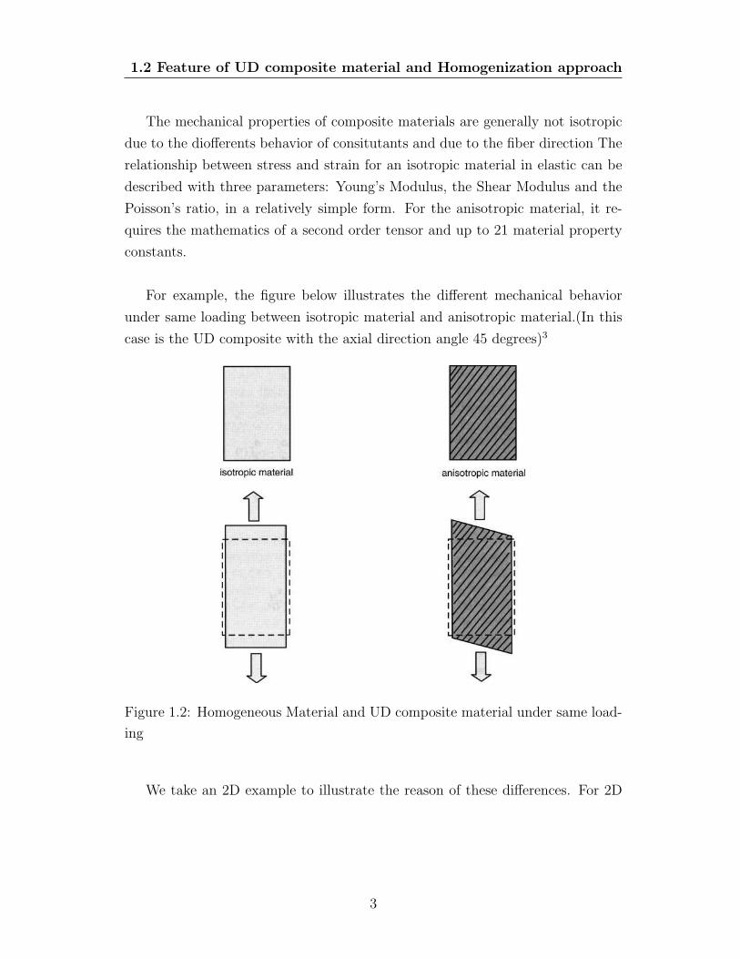
For example, the figure below illustrates the different mechanical behavior
under same loading between isotropic material and anisotropic material.(In this
case is the UD composite with the axial direction angle 45 degrees)3
Figure 1.2: Homogeneous Material and UD composite material under same load-
ing
We take an 2D example to illustrate the reason of these differences. For 2D
3
1.2 Feature of UD composite material and Homogenization approach
problem. The relation below is valid for anisotropic and elastic material.1
εx
εy
γxy
=
1Ex
−νyx
Ey0
−νxy
Ex
1Ey
0
0 0 1Gxy
σx
σy
τxy
From the equation, we can find that, for anisotropic material, to predict the
mechanical property with more precision in behavior,we need to more parameter.
1.2.2 Introduction of Concept of RVE
The homogenization procedure usually contain introduction of two scales, Marcro-
scale and Micro Scale, Marco-scale is usually refer to a homogenized continuous
medium, and micro-scale is usually related to a statistically representative vol-
ume element11 (RVE originally introduced by Hill 1963).Instead of predicting the
mechanical property of composite, we use homogenization technique and consid-
eration of RVE to predict the overall property from microscopic level.
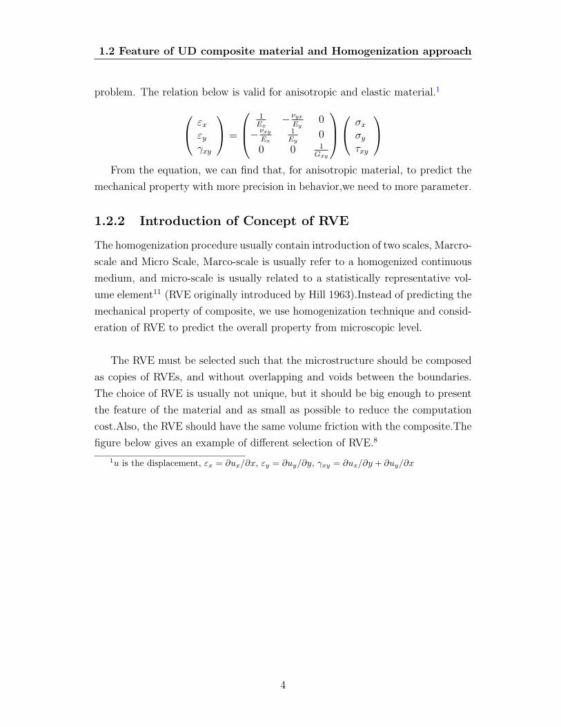
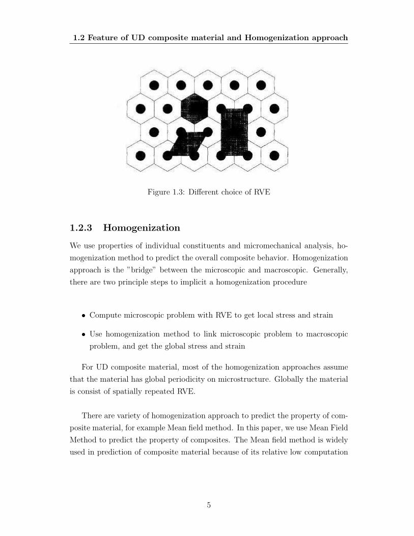
The RVE must be selected such that the microstructure should be composed
as copies of RVEs, and without overlapping and voids between the boundaries.
The choice of RVE is usually not unique, but it should be big enough to present
the feature of the material and as small as possible to reduce the computation
cost.Also, the RVE should have the same volume friction with the composite.The
figure below gives an example of different selection of RVE.8
1u is the displacement, εx = ∂ux/∂x, εy = ∂uy/∂y, γxy = ∂ux/∂y + ∂uy/∂x
4
1.2 Feature of UD composite material and Homogenization approach
Figure 1.3: Different choice of RVE
1.2.3 Homogenization
We use properties of individual constituents and micromechanical analysis, ho-
mogenization method to predict the overall composite behavior. Homogenization
approach is the ”bridge” between the microscopic and macroscopic. Generally,
there are two principle steps to implicit a homogenization procedure
• Compute microscopic problem with RVE to get local stress and strain
• Use homogenization method to link microscopic problem to macroscopic
problem, and get the global stress and strain
For UD composite material, most of the homogenization approaches assume
that the material has global periodicity on microstructure. Globally the material
is consist of spatially repeated RVE.
There are variety of homogenization approach to predict the property of com-
posite material, for example Mean field method. In this paper, we use Mean Field
Method to predict the property of composites. The Mean field method is widely
used in prediction of composite material because of its relative low computation
5

1.2 Feature of UD composite material and Homogenization approach
cost which enable us to use implicit constitutive laws in large scale simulations.
With the using of homogenization approach and RVE, we need to pay atten-
tion to following two points.
• The proper selection of RVE
• Because of periodicity of RVE, proper boundary condition should be se-
lected.
1.2.4 Boundary conditions
Periodic Boundary condition are imposed on RVE, and the choice of this bound-
ary conditions has been justified by a number of researchers.They prove that, by
applying periodic boundary condition, we can get more reasonable result compare
with other boundary conditions like stress uniform boundary condition(SUBC) or
kinematic uniform boundary conditions(KUBC). A typical RVE with Periodicity
is showed in below.11
Figure 1.4: A typical RVE with periodic boundary conditions
The periodic boundary conditions imply the following two fact:
• On the opposite surface, the deformation and the orientation should be
same
6

1.3 Computational Homogenization
• In order to have stress continuity across the boundaries the stress vectors
acting on opposite sides are opposite in direction.
u = Ex + u∗ u∗ is a periodic function
Take the RVE of figure 1.4 as an example. We consider the points on the
boundaries Γ14, Γ23.
u(xΓ14) = ExΓ14
+ u∗(xΓ14) (1.1)
u(xΓ23) = ExΓ23
+ u∗(xΓ23) (1.2)
Use 1.2-1.1, we have
u(xΓ23) − u(xΓ14
) = E(xΓ23− xΓ14
) (1.3)
More generally, we have A and B are two points on the opposite surface of
RVE.Then we have periodic boundary conditions as followed
u(xB) = u(xA) + E(xB − xA) or (1.4)
u(xB) − u(xA) = E(xB − xA) A,B onΓ (1.5)
ε(u(x)) = E + ε(u∗(x)), u∗ periodic (1.6)
Now we introduce the brackets 〈.〉 denote the volume average of a field V .
〈f〉 =1
|V |
∫
V
f(x) dx
1.3 Computational Homogenization
1.3.1 Initial boundary condition for Microscopic level
In the microscopic level, the material should satisfy the equations below
7

1.3 Computational Homogenization
∇ · σ = 0 inΩ (equilibrium equations) (1.7)
σij = Lijklεkl inΩ (constitutive equations) (1.8)
εij = ui,xjinΩ (Kinematic equations) (1.9)
ui = ui onΓu (Displacement boundary conditions) (1.10)
σij = ti onΓi (Traction boundary condition) (1.11)
u(xB) − u(xA) = E(xB − xA)
A,BonΓ (Periodic boundary conditions)(1.12)
1.3.2 Coupling of Microscopic and Macroscopic scales
In classical lamination theory the composite lamina is considered as a homoge-
neous orthotropic material with effective modulus that describe the overall me-
chanical property of composite. To obtain this macroscopic modulus, a homoge-
nization procedure are introduced during the computing linking the microscopic
scale and the macroscopic scale.
One of the mostly used method for homogenization is doing an volume inte-
gration over the RVE to averaging the stress and strain tensor:
σij =1
V
∫
V
σij(x, y, z) dV (1.13)
εij =1
V
∫
V
εij(x, y, z) dV (1.14)
We need to demonstrate that this procedure can keep the equivalence of strain
energy between the heterogeneous composite and the homogeneous composite
from averaging the stress and strain.In order to demonstrate the equivalence of
the energy, we assume that we have boundary traction ti and boundary displace-
ment ui.
The strain energy in a homogeneous material with volume V is:
U =1
2σijεijV (1.15)
8
1.3 Computational Homogenization
The strain energy stored in the heterogeneous material of volume V is:
U ′ = 12
∫
Vσijεij V (1.16)
U ′ = 12
∫
Vσij(εij + εij − εij) V (1.17)
= 12
∫
Vσij(εij − εij) V + 1
2εij
∫
Vσij V (1.18)
As we have illustrated in Equation 1.13, so we have
U ′ = 12
∫
Vσij(εij − εij) V + 1
2σijεijV (1.19)
= 12
∫
Vσij(εij − εij) V + U (1.20)
U ′ − U = 12
∫
Vσij(
∂ui
∂xj− ∂ui
∂xj) V (1.21)
= 12
∫
V[∂σij
∂xj(ui − ui) +
∂(σij(ui−ui))
∂xj] V (1.22)
Use the equilibrium equation
∂σij
∂xj
= 0
We can write the energy difference as
U ′ − U =1
2
∫
V
∂
∂xj
[σij(ui − ui)] V (1.23)
By using Gauss theorem we can transform the integration of the volume into
the integration of the surface
U ′ − U =1
2
∫
S
σij(ui − ui)nj S (1.24)
S is the surface of the RVE, and n denote the unit outward normal vector
and On the surface S, we have
ui = ui
So we have conclusion that
U = U ′
The derivation above showed that, the homogenization we used ensure the
equivalence between the heterogeneous RVE and the homogenized RVE.
9
Chapter 2
Implement Homogenization in
Abaqus
2.1 Introduction of implementation
In order to implement the Periodic Boundary Conditions in Abaqus, we need to
use constrain functions in Abaqus, however, this functions is designed for points
constrain only. To apply this BC on the all boundaries of the model, we need
to creates hundreds of constrain equations for every couple of points on the cor-
responding surfaces. Considering the scale of the problem, it’s not realistic to
create the constrain equations manually.
Abaqus Scripting Interface(API) enable us to costmize the Abaqus ourselves.
With the API, we can
• Automate repetitive tasks
• Extend functionality
• Enhance the interface
Creating the constrain equations is a kind of repetitive task, so it is possible
to do that with API.
10

2.1 Introduction of implementation
Python is the standard programming language for ABAQUS products, it has
a very good compatibility with Abaqus.In Abaqus,
• The ABAQUS environment file uses Python statements.
• The parameter definitions on the data lines of the *PARAMETER option
in the ABAQUS input file are Python statements.
• The parametric study capability of ABAQUS requires the user to write and
to execute a Python scripting (.psf) file.
• ABAQUS/CAE records its commands as a Python script in the replay
(.rpy) file.
• You can execute ABAQUS/CAE tasks directly using a Python script.
• You can access the output database (.odb) using a Python script.
And Python is an interpreted language. This means you can type a statement
and view the results without having to compile and link your scripts. Experi-
menting with Python statements in Abaqus is quick and easy.9
These advantages make Python the best programming language for creating
scripts for Abaqus.
In this chapter, we are going to illustrate how to implement homogenization
procedure in Abaqus and give some demonstrations of validity.First we are going
to have some preview of Python language, after that, the constrain equation
function in Abaqus will be introduced. Then, the general structure of Python
scripts will be given, at last, some demonstration will be given to proof the validity
of the method.
11

2.2 Use Python scripts to implement homogenization
2.2 Use Python scripts to implement homoge-
nization
2.2.1 Abaqus Scripting Interface and Python
The Abaqus Scripting Interface is an application programming interface (API)
to the models and data used by Abaqus. The Abaqus Scripting Interface is an
extension of the Python object-oriented programming language; Abaqus Scripting
Interface scripts are Python scripts. You can use the Abaqus Scripting Interface
to do the following:9
• Create and modify the components of an Abaqus model, such as parts,
materials, loads, and steps.
• Create, modify, and submit Abaqus analysis jobs.
• Read from and write to an Abaqus output database.
• View the results of an analysis.
In Abaqus, there is no option for applying periodic boundary conditions.
Python scripts enable us to implement Homogenization procedure in Abaqus
for composite material.In order to do that, we need to create a python scripts
which should include following functions (This Python scripts inquire the RVE
should be cuboid)
• Read the mesh database and find the boundaries
• Scan the geometry model and find opposite surfaces
• Pick up corresponding coordinates of opposite surfaces from mesh database
• create reference points to implement homogenization approach
• create constrain equations for applying periodic boundary conditions
12

2.2 Use Python scripts to implement homogenization
2.2.2 Constrain equations for periodic boundary condi-
tions
In Interaction module of Abaqus, we can define different kind of interactions
between parts of the model or inside the model. In constrain submodule, it
provide a possibility to create a linear equation constraint by entering data in
the Edit Constraint dialog box. The terms of an equation consist of a coefficient
applied to a degree of freedom of every node in a set.
A linear multi-point constraint requires that a linear combination of nodal
variables is equal to zero; that is,
A1uPi + A2u
Qj + · · · + ANuR
k = 0
Where uPi is a nodal variable at node P, degree of freedom i, and the An are
coefficients that define the relative motion of the node.In general, we need to
specify following parameters to define a linear constraint equation
• the number of terms in the equation, N
• the nodes, P , and the degrees of freedom, i, corresopnding to the nodal
variables uPi
• coefiicients, An
For example, to impose the equation
u21 − u3
2 − 2u15 = 0 ui is the displacement of point i
We need to define three point set to contain point1,point3 and point5. Use
python command
mdb.models[ModelName].rootAssembly.Set(’pointset1’,nodes=Noeuds[(location
in the database)])
Then use command
13

2.2 Use Python scripts to implement homogenization
mdb.models[ModelName].Equation(name=Constraintname,terms=((1.0,’pointset1’,2),(-
1.0,’pointset2’,3),(-2,”pointset3,1)))
to creat the linear constrain illustrate above, we use loops to read the database,
and create the constrain equations automatically.
In our model for 3D cuboid RVE, we need to apply periodic boundary condi-
tion 1.6 to the computation, We have Macroscopic strain matrix E = Eij i, j =
1, 2, 3. In order to include Macroscopic strain component Eij, we can create six
reference point RP-1, RP-2 ... RP-6. Their displacement of degree of freedom
one stand for E11, E12, E13, E22, E23, E33 respectively.1
U1RP−1 = E11
...
U1RP−6 = E33
By introducing six reference points, we can apply periodic boundary condi-
tions by creating constrain equations using the python command above in Abaqus.
2.2.3 Validly of homogenization procedure
In this chapter,we are going to demonstrate that the introduction of six reference
could give correct output for macroscopic strain.
To verify the accuracy of the output of macroscopic strain from the displace-
ment of reference points, we need to demonstrate that the displacement of ref-
erence points are exactly the integration of local strain over the RVE. Take the
RVE in fig as an example.
1u is the macro displacement, E11 = ∂ux/∂x, E22 = ∂uy/∂y, E12 = (∂ux/∂y + ∂uy/∂x)/2
14
2.2 Use Python scripts to implement homogenization
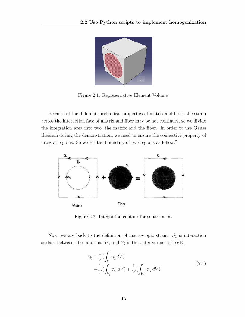
Figure 2.1: Representative Element Volume
Because of the different mechanical properties of matrix and fiber, the strain
across the interaction face of matrix and fiber may be not continues, so we divide
the integration area into two, the matrix and the fiber. In order to use Gauss
theorem during the demonstration, we need to ensure the connective property of
integral regions. So we set the boundary of two regions as follow:2
Figure 2.2: Integration contour for square array
Now, we are back to the definition of macroscopic strain. S1 is interaction
surface between fiber and matrix, and S2 is the outer surface of RVE.
εij =1
V(
∫
V
εij dV )
=1
V(
∫
Vf
εij dV ) +1
V(
∫
Vm
εij dV )(2.1)
15
2.2 Use Python scripts to implement homogenization
Use Gauss theorem, transform the integration of volume to the surface inte-
gration
εij =1
V(1
2
∫
S1
(uinj + ujni) dS))
+1
V(1
2
∫
S2
(uinj + ujni) dS) −1
2
∫
S1
(uinj + ujni) dS))
(2.2)
So we can get the volume integration of local strain from the displacement of
boundary
εij =1
V
∫
S2
(uinj + ujni) dS (2.3)
We assume we are using triangle element mesh, and first order shape function
in the finite element computing. We are going to prove that if Eij satisfy the
constrain equation 1.6, Eij is equal to the volume integration of εij. We take E11
as an example to demonstrate the validity. The RVE model is showed in Fig 2.1
, with lenght, width, and height α, β, γ respectively.
In this Case, we have
uA − uB = αE11 (2.4)
for every point on surface A and B.
In finite element analysis, we use linear combination of shape function to
describe the displacement function. Within a 3-noded triangular element we can
interpolate the displacement as:
U = U1N1 + U2N2 + U3N3 (2.5)
16

2.2 Use Python scripts to implement homogenization
Figure 2.3: Shape functions
Where n1, N2, N3 are shape functions illustrated in Fig 2.3 They are linear
unctions of nondimensional coordinates ξ and η
N1 = ξ, N2 = η, N3 = 1 − ξ − η (2.6)∫
ΩNi ds = 1
3SΩ (2.7)
We start from one of the element Ae on the surface of A, and with the area
Se,because of the symmetric of mesh, on the opposite side, we have an element Be
which has the same shap with Ae we assume that Ωe = Ae ∪ Be. In element Ωe,
we have constrain equations from the periodic boundary conditions we applied in
the Abaqus.
uAi − uBi = αE11 i = 1, 2, 3 inΩe (2.8)
And
uA =∑n
i=1 uAiNi in Ae (2.9)
uB =∑n
i=1 uBiNi in Be (2.10)
Equations 2.8 multiply 13Se ⇒
uAi
1
3Se − uBi
1
3Se =
1
3SeαE11 i = 1, 2, 3 (2.11)
17

2.2 Use Python scripts to implement homogenization
Because we have 2.7,
N1 = ξ, N2 = η, N3 = 1 − ξ − η (2.12)∫
ΩNi ds = 1
3SΩ (2.13)
substitude formula 2.7 into equation2.11, we have
∫
Ae
uAiNi ds −
∫
Be
uBiNi ds = SeαE11 i = 1, 2, 3 (2.14)
Because the normal vector of surface A and B are opposite, nA = (1, 0, 0) nB =
(−1, 0, 0) So, we can write 2.14 as
∫
Ωe
uAiNi − uBiNi ds = SeαE11 i = 1, 2, 3 (2.15)
Use relation 2.9,2.10 and sum these three equation, we get∫
Ωe
uA − uB ds = SeαE11 ⇒ (2.16)
Sum all the element Ωe on the surface A and B, we get the equation for the whole
surface.
∫
Ωu1n1 ds = V E11 ⇒ (2.17)
E11 = 1V
∫
S2
u1n1 ds ⇒ (2.18)
εij = E11 (2.19)
The prove for other component of Eij is similar. This prove enable us to
compute the value of Eij in the constrain equation instead of computing the
volume integration in homogenization procedure.
2.2.4 Equation elimination
To apply the periodic boundary conditions, we need to convert the boundary
conditions on the surface into point constrain equations on mesh points. How-
ever, during this procedure, we may have some extra equations which could be
derived by other equations. Solving the equation systems without eliminating
these extra equations could cause singular matrix calculation. Although in some
18

2.2 Use Python scripts to implement homogenization
software, they can deal with this kind of cases automatically, but in Abaqus, en-
tering equation systems with extra formulas will cause error. So we need to avoid
such situation and it is necessary to explore our constrain equation systems, and
eliminate extra equations.
We start with 2D single fiber RVE model. And we can see why we need to
eliminate the extra equations. Suppose we have a RVE, length and width are α
and β respectively. Now, we consider equations of four coner points:
uB1 − uA1 = αE11 (2.20)
uB2 − uA2 = αE12 (2.21)
uC1 − uD1 = αE11 (2.22)
uC2 − uD2 = αE12 (2.23)
uA1 − uD1 = βE12 (2.24)
uA2 − uD2 = βE22 (2.25)
uB1 − uC1 = βE12 (2.26)
uB2 − uC2 = βE22 (2.27)
Degree freedom 1 and degree freedom 2 are independent to each other.We
take the solving of DOF 1 as an example to show the necessary of elimination.
uB1 − uA1 = αE11 (2.28)
uC1 − uD1 = αE11 (2.29)
uA1 − uD1 = βE12 (2.30)
uB1 − uC1 = βE12 (2.31)
Write it into matrix form:
−1 1 0 00 0 1 −11 0 0 −10 1 −1 0
uA1
uB1
uC1
uD1
=
αE11
αE11
βE12
βE12
(2.32)
19

2.2 Use Python scripts to implement homogenization
We can find that the matrix on the left is a singular matrix. So it’s not pos-
sible to do the matrix calculation to get the value of u.
Using elimination to avoid the singular matrix.
uB1 − uC1 = uB1 − uA1 + uA1 − uD1 + uD1 − uC1
= αE11 + βE12 − βE12
= αE11
(2.33)
Equation2.28,Equation2.30,Equation2.31⇒ Equation2.29
uB2 − uC2 = uB2 − uA2 + uA2 − uD2 + uD2 − UC2
= αE12 + βE22 − βE22
= αE12
(2.34)
Equation2.21,equation2.25,equation2.27 ⇒ equation2.23
From the derivation above, we can eliminate two extra equations from the
system Now, we extend our solution to 3D case. Consider a RVE single fiber
model in Fig2.1.
We categorise the mesh points into three sorts:
• points on the surface but not on the edges and corner
• points on the edges but not on corner
• points on the corner
For the points on the surface, the equation system is unique, there are no
extra equations in the system. For the points on the edges, we can consider it
as 2D problem, take the Fig as an example, Points A,B,C,D could be looked as
point on four corners of a square, then we can use the solution above to eliminate
two extra equations.
The elimination for corner points of a cuboid will be more complex. In this
case, we have eight points to be considered: a, b, c, d, k, l,m, n. And the length ,
20
2.2 Use Python scripts to implement homogenization
width and height are α, β, γ respectively. To simplify the demonstration, we take
degree of freedom 1 as an example.
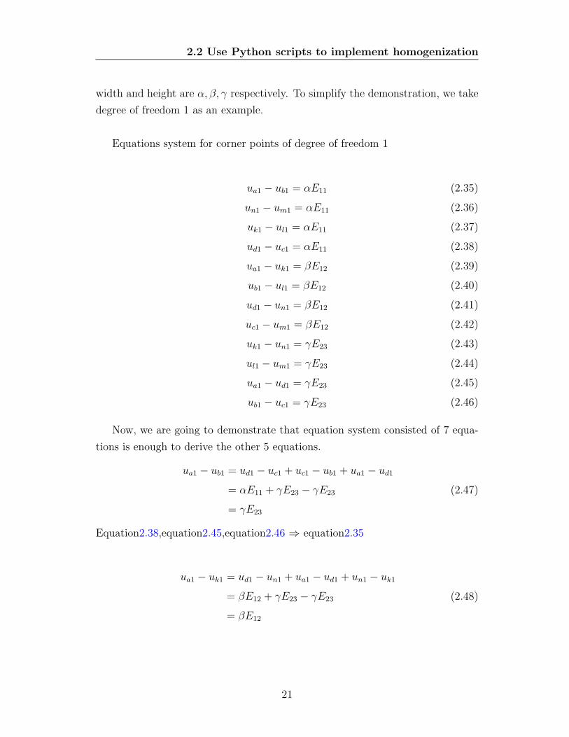
Equations system for corner points of degree of freedom 1
ua1 − ub1 = αE11 (2.35)
un1 − um1 = αE11 (2.36)
uk1 − ul1 = αE11 (2.37)
ud1 − uc1 = αE11 (2.38)
ua1 − uk1 = βE12 (2.39)
ub1 − ul1 = βE12 (2.40)
ud1 − un1 = βE12 (2.41)
uc1 − um1 = βE12 (2.42)
uk1 − un1 = γE23 (2.43)
ul1 − um1 = γE23 (2.44)
ua1 − ud1 = γE23 (2.45)
ub1 − uc1 = γE23 (2.46)
Now, we are going to demonstrate that equation system consisted of 7 equa-
tions is enough to derive the other 5 equations.
ua1 − ub1 = ud1 − uc1 + uc1 − ub1 + ua1 − ud1
= αE11 + γE23 − γE23
= γE23
(2.47)
Equation2.38,equation2.45,equation2.46 ⇒ equation2.35
ua1 − uk1 = ud1 − un1 + ua1 − ud1 + un1 − uk1
= βE12 + γE23 − γE23
= βE12
(2.48)
21
2.2 Use Python scripts to implement homogenization
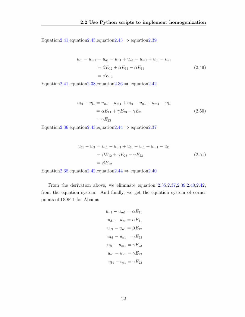
Equation2.41,equation2.45,equation2.43 ⇒ equation2.39
uc1 − um1 = ud1 − un1 + un1 − um1 + uc1 − ud1
= βE12 + αE11 − αE11
= βE12
(2.49)
Equation2.41,equation2.38,equation2.36 ⇒ equation2.42
uk1 − ul1 = un1 − um1 + uk1 − un1 + um1 − ul1
= αE11 + γE23 − γE23
= γE23
(2.50)
Equation2.36,equation2.43,equation2.44 ⇒ equation2.37
ub1 − ul1 = uc1 − um1 + ub1 − uc1 + um1 − ul1
= βE12 + γE23 − γE23
= βE12
(2.51)
Equation2.38,equation2.42,equation2.44 ⇒ equation2.40
From the derivation above, we eliminate equation 2.35,2.37,2.39,2.40,2.42,
from the equation system. And finally, we get the equation system of corner
points of DOF 1 for Abaqus
un1 − um1 = αE11
ud1 − uc1 = αE11
ud1 − un1 = βE12
uk1 − un1 = γE23
ul1 − um1 = γE23
ua1 − ud1 = γE23
ub1 − uc1 = γE23
22

2.2 Use Python scripts to implement homogenization
For degree of freedom 2 and 3, the elimination is exactly the same. Now, we
have considered all the mesh points on the surface of RVE. The equation system
now is ready to be input in Abaqus by Python scripts.
2.2.5 Brief instruction of the use of Python scripts
With the preparation above, here gives the general structure of the use of Python
Scripts for applying periodic boundary conditions and homogenization procedure.
Figure 2.4: Instruction of use of Python Scripts
The complete code with comments could be found at the appendix of this
paper.
To use this python scripts, you need to create a .CAE file in Abaqus, with ge-
ometry, material property of fiber and matrix, symmetric mesh and macroscopic
loading. Then run Python scripts in Abaqus, the scripts will add the reference
points, create the constrain equations automatically. When the scripts is done,
run the simulation in Abaqus, then you can get the result from Visualization. Mi-
croscopic strain and stress could be export from Abaqus database, macroscopic
stress is the initial condition used input, and macroscopic strain are the displace-
ment of DOF 1 of six reference points. Now, a homogenization simulation for
composite material is complete.
23

Chapter 3
Numerical simulation and
experment
3.1 Experiment for UD composite
Some experiment has been done for single layer UD composite laminar. The
component of the composite is epoxy (Matrix) and E-glass (fiber). The friction
volume is 57% ± 3% The mechanical property of constituent3
Constituent Young’s modulus E Poisson ratio ν
Epoxy 977-20 3GPa 0.4
E Glass 74GPa 0.26
Table 3.1: Elastic constant
And harding law for Matrix:
GNUPLOT
We are going to do three experiment to the single composite laminar. They
are showed as below:
• Fiber along with x direction
• Fiber along with y direction
24
3.2 Numerical result
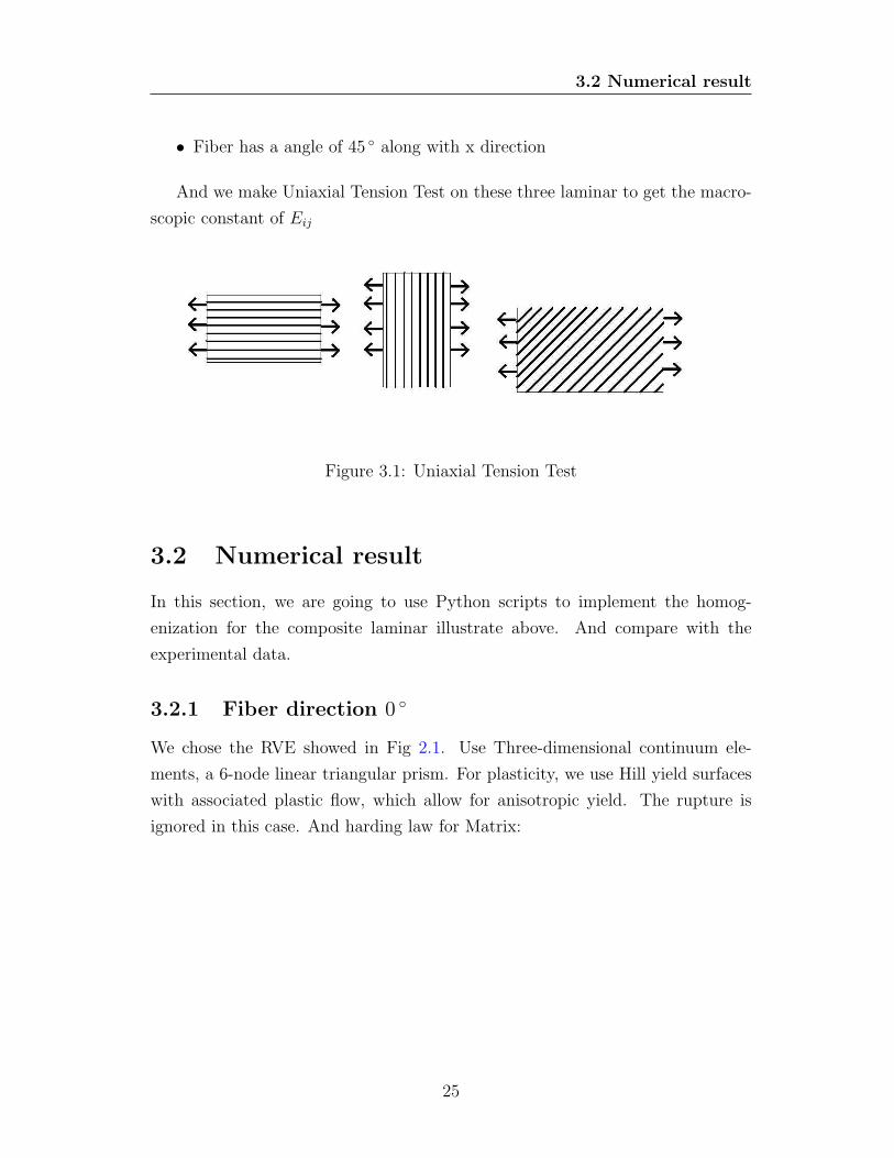
• Fiber has a angle of 45 along with x direction
And we make Uniaxial Tension Test on these three laminar to get the macro-
scopic constant of Eij
Figure 3.1: Uniaxial Tension Test
3.2 Numerical result
In this section, we are going to use Python scripts to implement the homog-
enization for the composite laminar illustrate above. And compare with the
experimental data.
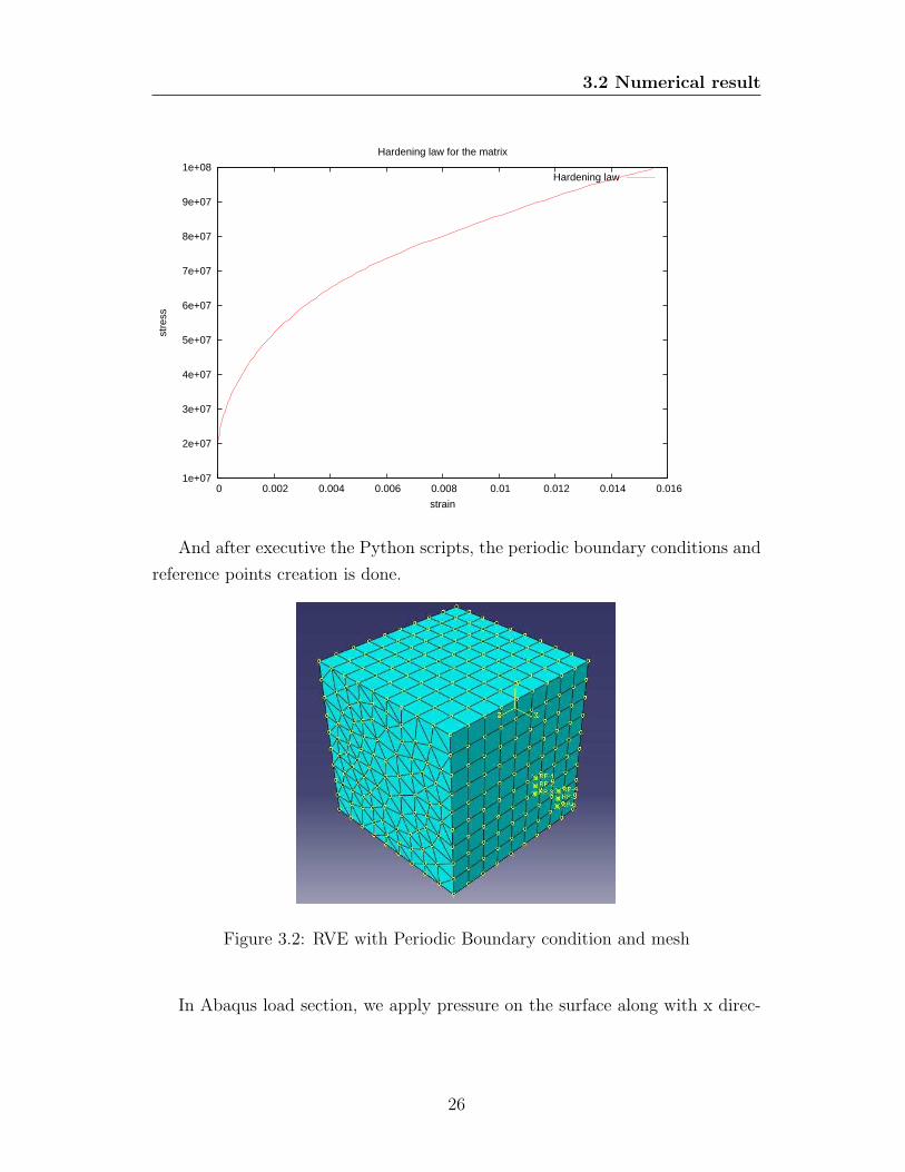
3.2.1 Fiber direction 0
We chose the RVE showed in Fig 2.1. Use Three-dimensional continuum ele-
ments, a 6-node linear triangular prism. For plasticity, we use Hill yield surfaces
with associated plastic flow, which allow for anisotropic yield. The rupture is
ignored in this case. And harding law for Matrix:
25
3.2 Numerical result
1e+07
2e+07
3e+07
4e+07
5e+07
6e+07
7e+07
8e+07
9e+07
1e+08
0 0.002 0.004 0.006 0.008 0.01 0.012 0.014 0.016
stre
ss
strain
Hardening law for the matrix
Hardening law
And after executive the Python scripts, the periodic boundary conditions and
reference points creation is done.
Figure 3.2: RVE with Periodic Boundary condition and mesh
In Abaqus load section, we apply pressure on the surface along with x direc-
26
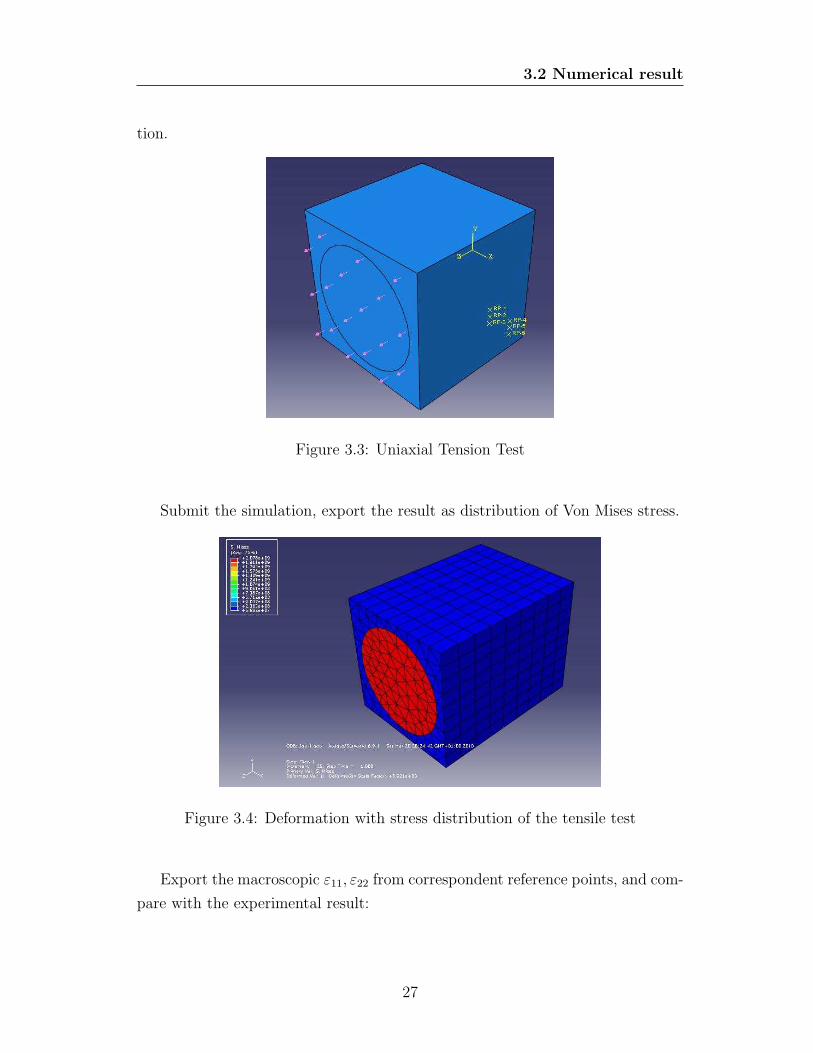
3.2 Numerical result
tion.
Figure 3.3: Uniaxial Tension Test
Submit the simulation, export the result as distribution of Von Mises stress.
Figure 3.4: Deformation with stress distribution of the tensile test
Export the macroscopic ε11, ε22 from correspondent reference points, and com-
pare with the experimental result:
27

3.2 Numerical result
σ11(MPa) ε11(%) ε22(%) E11(MPa) ν12
numerical result 1200 2.802 -0.898 43034.8 -0.3132
Experimental data 1252 2.78 -0.89 45043 0.311
Table 3.2: Result comparison of longitudinal Young’s modulus
From the figure of strain stress curve, we can find that, the numerical result
match the experimental data very well at the beginning, and the error occurs
when the strain increase. This error comes from the lack of consideration of
rupture in the simulation. As the strain and stress increase, some crack will
appear in the matrix as well as in the section between matrix and fiber.And from
the plot, we can also discover that, the behavior is linear, the fiber reinforce the
material efficiently.
0
200
400
600
800
1000
1200
1400
0 0.5 1 1.5 2 2.5 3
stre
ss
strain
E11 for RVE with fiber direction 0 degree
Numerical resultExperimental result
28
3.2 Numerical result
0
200
400
600
800
1000
1200
1400
-0.9 -0.8 -0.7 -0.6 -0.5 -0.4 -0.3 -0.2 -0.1 0
stre
ss
strain
E22 for RVE with fiber direction 0 degree
Numerical resultExperimental result
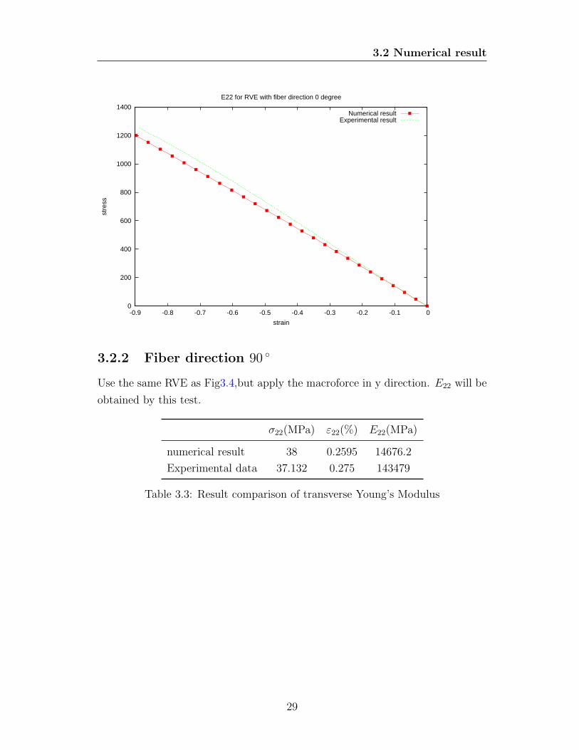
3.2.2 Fiber direction 90
Use the same RVE as Fig3.4,but apply the macroforce in y direction. E22 will be
obtained by this test.
σ22(MPa) ε22(%) E22(MPa)
numerical result 38 0.2595 14676.2
Experimental data 37.132 0.275 143479
Table 3.3: Result comparison of transverse Young’s Modulus
29

3.2 Numerical result
0
5
10
15
20
25
30
35
40
0 0.05 0.1 0.15 0.2 0.25 0.3
stre
ss
strain
E22 for RVE with fiber direction 90 degree
Numerical resultExperimental result
Transverse tensile test shows similar phenomenon as longitudinal test. The
prediction agrees the experimental data well at small strain area, then error grows
as the strain increase. And the behavior is still near linear.
3.2.3 Fiber direction 45
Now we have got the transverse and longitudinal modulus, we are going to de-
sign a test for finding out shear modulus. We test composite laminar with fiber
direction 45 , as the composite is anisotropic, when we apply transverse load, it
will also give shear strain. We can use coordinate transformation to calculate the
shear modulus.
The RVE 2.1 used for previous test does not appropriate now, we use RVE
below:
30

3.2 Numerical result
Figure 3.5: RVE for composite laminar with fiber direction 45
To get G12, we need to do axes transform for strain and stress.Suppost we
have known the stress and strain on xy planes, but we want to stresses acting on
planes oriented at θ, We will propose a means to transform the stresses to these
new x′y′ planes.
Figure 3.6: Axes transformation for strain and stress
In our case, for the composite laminar as Fig 3.7 below, we know the σ ε
in xy direction, but we want to use transformation of axes to get σ ε in fiber
direction, which has an angle θ with the original coordinates.
31

3.2 Numerical result
Figure 3.7: Axes transformation for UD composite laminar
We have solution for the problem:
σx′
σy′
τx′y′
=
c2 s2 2scs2 c2 −2sc−sc sc c2 − s2
σx
σy
τxy
(3.1)
Where s = sinθ, c = cosθ, and we set matrix A as the transformation matrix
above, we can write transformation as
σ′ = Aσ (3.2)
and for strain transformation
εx′
εy′
12γx′y′
= A
εx
εy12γxy
(3.3)
Use the conclusion of axes transformation above, we can calculate the corre-
sponding pressure value from the experiment and apply it on our RVE.When the
computing is done, we use transformation to get εx′ , εy′andεx′y′ .
Computational result
32

3.2 Numerical result
Figure 3.8: Computational result for laminar with 45
Elastic modulus
G12(MPa) E22(MPa)
numerical result 3696.58 7834.466
Experimental data 3755 9618
Table 3.4: Result comparison of shear modulus
For the plasticity, we can compare the result by strain stress curve.
33

3.2 Numerical result
0
5
10
15
20
25
30
35
40
45
-0.2 0 0.2 0.4 0.6 0.8 1 1.2 1.4 1.6 1.8 2
stre
ss
strain
G12 for RVE with fiber direction 45 degree
Numerical resultExperimental result
0
5
10
15
20
25
30
35
40
45
-0.1 0 0.1 0.2 0.3 0.4 0.5 0.6
stre
ss
strain
E22 for RVE with fiber direction 45 degree
Numerical resultExperimental result
In the result we can find, for shear strain stress curve, the model can match
the experiment curve very well at elastic strain and small plastic strain area. but
34

3.2 Numerical result
the error becomes big after that for the model without damage introduction. In
this case, damage is a significant parameter to affect the evolution of the material,
however, in Abaqus, only linear damage parameter law or exponential damage
parameter law is available for the model. In this two damage laws, both require
the damage parameter start from 0 and end at 1. And both of them is not for
this case.1. This problem could be solved by introducing User Subroutine which
enable the user to introduce the damage law themselves.
1The experiment shows that, for this kind of UD composite, the damage parameter law is
linear, but not start from 0 and also not end with 1
35
Chapter 4
Conclusion
The aim of this paper is to introduce Homogenization method to widely used
commercial software Abaqus, to enable it to estimate the overall mechanical be-
havior of UD composite material.
We first shortly introduce the history of composite material, the feature of
composite material and concept of UD composite. Due to the outstanding me-
chanical performance of composite, it’s important to develop a reliable and eco-
nomic numerical method to estimate the overall mechanical parameters of com-
posite from the component material. A brief review of method of estimation of
parameter of composite are given. In this paper, we are going to use homogeniza-
tion method to evaluate the mechanical property of composite.The key difficults
of predicting mechanical parameter of composite with Abaqus are appying peri-
odic boundary conditions and homogenization procedure from microscopic level
to macroscopic level.
After that, concepts RVE, periodic boundary conditions which are related
with homogenization method are introduced. And some detailed derivation is
also presented. In order to valid the homogenization method in FEM, concepts
of Scripts interface, features of commercial FEM software Abaqus and Python
object oriented programming language are presented. The task of the scripts is to
enable Abaqus to apply periodic boundary conditions to the model and execute
the homogenization procedure. The algorithm and structure of implementation
36
using Python in Abaqus are showed in the second chapter. At last part of the
article, some numerical example are done by Abaqus with Python scripts. And
the numerical result are compared with experimental data to verify the validation
of the code.
According to the comparison of numerical result and experimental data. We
can conclude that, predicting the mechanical parameter of UD composite materiel
by homogenization method is possible in Abaqus. It could be done by using
Python scripts in Abaqus. Some proof has been done to verify the correctness
theoretically. And numerical test showed the reliability of this scripts as well
as the validity. So we can conclude that, using Python scripts, it’s possible to
predict the mechanical parameter of elasticity and plasticity of UD composite
material safely. But the error increase as the strain grows because of the lack
of consideration of interaction between fiber and matrix as well as appropriate
damage law during the computing.And the existing scripts is only valid for simple
geometry model. In the future research, dealing with complex geometry model
and including the interaction between fiber and matrix could be considered. And
using User Subroutine to introduce appropriate damage law could also be done
to improve the model.
37

Appendix A
Python Scripts
from abaqus import∗ from abaqusConstants import ∗
ModelName=’Model−1 ’ # Input data InstanceName=’Part−1−1’Noeuds=mdb. models [ ModelName ] . rootAssembly .i n s t an c e s [ InstanceName ] . nodes
# Get the dimensions o f the square model # note : next s t ep => t r yto f i nd the type o f VER and automatise the p roce s sNb−noeuds=len (Noeuds ) Max−x=−1000 Max−y=−1000 Min−x=1000 Min−y=1000Max−z=−1000 Min−z=1000 rad iu s=100 cen=0
for i in range (Nb−noeuds ) :Cx= Noeuds [ i ] . c oo rd ina t e s [ 0 ]Cy= Noeuds [ i ] . c oo rd ina t e s [ 1 ]Cz= Noeuds [ i ] . c oo rd ina t e s [ 2 ]i f Max−x<=Cx :
Max−x=Cxi f Cx <=Min−x :
Min−x=Cxi f Max−y<=Cy :
Max−y=Cyi f Cy <=Min−y :
Min−y=Cy
38

i f Max−z<=Cz :Max−z=Cz
i f Cz <=Min−z :Min−z=Cz
lx=Max−x−Min−x ly=Max−y−Min−yl z=Max−z−Min−z l x c=(Max−x+Min−x )/2l y c=(Max−y+Min−y )/2 l z c =(Max−z+Min−z )/2
for i in range (Nb−noeuds ) :Cx= Noeuds [ i ] . c oo rd ina t e s [ 0 ]Cy= Noeuds [ i ] . c oo rd ina t e s [ 1 ]Cz= Noeuds [ i ] . c oo rd ina t e s [ 2 ]i f (Cx−l x c )∗ (Cx−l x c )+(Cy−l y c )∗ (Cy−l y c )+(Cz−l z c )∗ (Cz−l z c )
<=rad iu s :cen=irad iu s=(Cx−l x c )∗ (Cx−l x c )+(Cy−l y c )∗ (Cy−l y c )+(Cz−l z c )∗ (Cz−l z c )
# Stor ing o f nodes b e l ong ing to the e x t e r na l Faces # (Used f o r thetreatment o f c on s t r a i n t s equat ion ; important note : t h i s i s not
node l a b e l s to r ed but array index o f Noeuds ) Set−xDroite =[ ]Set−xGauche=[ ] Set−yHaut=[ ] Set−yBas =[ ] Set−zDro i te =[ ]Set−zGauche =[ ]
lSet−xDroite =[ ] lSet−xGauche=[ ] lSet−yHaut=[ ] lSet−yBas =[ ]lSet−zDro i te =[ ] lSet−zGauche =[ ]
for i in range (Nb−noeuds ) :Cx= Noeuds [ i ] . c oo rd ina t e s [ 0 ]Cy= Noeuds [ i ] . c oo rd ina t e s [ 1 ]Cz= Noeuds [ i ] . c oo rd ina t e s [ 2 ]
# Only s t r o r e the nodes i n c l u d e s in the cons t r a in s equa t i onsi f (Max−x==Cx) and (Cy!=Max−y ) and (not ( (Cy==Min−y )and (Cz==Max−z ) ) ) :
Set−xDroite . append ( i )lSet−xDroite . append ( i +1)
i f (Cx==Min−x ) and (Cy!=Max−y ) and (not ( (Cy==Min−y )and (Cz==Max−z ) ) ) :
39

Set−xGauche . append ( i )lSet−xGauche . append ( i +1)
i f (Max−y==Cy) and ( (Cz!=Max−z ) or ( (Cz==Max−z ) and
(Cx==Min−x ) ) or ( (Cz==Max−z ) and (Cx==Max−x ) ) )Set−yHaut . append ( i )lSet−yHaut . append ( i +1)
i f (Cy==Min−y ) and ( (Cz!=Max−z ) or ( (Cz==Max−z ) and
(Cx==Min−x ) ) or ( (Cz==Max−z ) and (Cx==Max−x ) ) ) :Set−yBas . append ( i )lSet−yBas . append ( i +1)
i f (Cz==Max−z ) and ( (Cx!=Max−x ) or ( (Cx==Max−x ) and
(Cy==Min−y ) ) ) and (not ( (Cx==Min−x ) and (Cy==Max−y ) ) ) :Set−zDro i te . append ( i )lSet−zDro i te . append ( i +1)
i f (Cz==Min−z ) and ( (Cx!=Max−x ) or ( (Cx==Max−x ) and
(Cy==Min−y ) ) ) and (not ( (Cx==Min−x ) and (Cy==Max−y ) ) ) :Set−zGauche . append ( i )lSet−zGauche . append ( i +1)
i f Cx∗Cx+Cy∗Cy+(Cz−1)∗(Cz−1)<=rad iu s :cen=irad iu s=(Cx−l x c )∗ (Cx−l x c )+(Cy−l y c )∗ (Cy−l y c )+(Cz−l z c )∗ (Cz−l z c )
# Creat ing the t h r e e r e f e r ence po in t s (macro nodes )mdb. models [ ModelName ] . rootAssembly . ReferencePoint( po int =(1 . 2 , 0 . 1 , 1 . 0 ) )mdb. models [ ModelName ] . rootAssembly . ReferencePoint( po int =(1 . 2 , 0 . 0 , 1 . 0 ) )mdb. models [ ModelName ] . rootAssembly . ReferencePoint( po int =(1 .2 , −0 .1 ,1 .0 ) )mdb. models [ ModelName ] . rootAssembly . ReferencePoint( po int =(1 . 5 , 0 . 1 , 1 . 0 ) )mdb. models [ ModelName ] . rootAssembly . ReferencePoint( po int =(1 . 5 , 0 . 0 , 1 . 0 ) )mdb. models [ ModelName ] . rootAssembly . ReferencePoint( po int =(1 .5 , −0 .1 ,1 .0 ) )
# Bu i l t the Se t s o f every f a c e s . I t ’ s convenience f o r check ing
40
mdb. models [ ModelName ] . rootAssembly . SetFromNodeLabels (name=’ setxd ’ , nodeLabels=(( InstanceName , ( 2 , 3 , 5 , 7 ) ) , ( InstanceName ,lSet−xDroite ) ) )
mdb. models [ ModelName ] . rootAssembly . SetFromNodeLabels (name=’ setxg ’ , nodeLabels=(( InstanceName , ( 2 , 3 , 5 , 7 ) ) , ( InstanceName ,lSet−xGauche ) ) )
mdb. models [ ModelName ] . rootAssembly . SetFromNodeLabels (name=’ setyh ’ , nodeLabels=(( InstanceName , ( 2 , 3 , 5 , 7 ) ) , ( InstanceName ,lSet−yHaut ) ) )
mdb. models [ ModelName ] . rootAssembly . SetFromNodeLabels (name=’ setyb ’ , nodeLabels=(( InstanceName , ( 2 , 3 , 5 , 7 ) ) , ( InstanceName ,lSet−yBas ) ) )
mdb. models [ ModelName ] . rootAssembly . SetFromNodeLabels (name=’ se tzd ’ , nodeLabels=(( InstanceName , ( 2 , 3 , 5 , 7 ) ) , ( InstanceName ,lSet−zDro i te ) ) )
mdb. models [ ModelName ] . rootAssembly . SetFromNodeLabels (name=’ s e t zg ’ , nodeLabels=(( InstanceName , ( 2 , 3 , 5 , 7 ) ) , ( InstanceName ,lSet−zGauche ) ) )
41
# Creat ing unique s e t f o r the prev ious i d e n t i f i e d nodesSet−name=’ Set−N’
for i in range ( l en ( Set−xDroite ) ) :mdb. models [ ModelName ] . rootAssembly . Set (name=Set−name+’xD ’+s t r ( i ) , nodes=Noeuds [ Set−xDroite [ i ] : Set−xDroite [ i ]+1 ] )
for i in range ( l en ( Set−xGauche ) ) :mdb. models [ ModelName ] . rootAssembly . Set (name=Set−name+’xG ’+s t r ( i ) , nodes=Noeuds [ Set−xGauche [ i ] : Set−xGauche [ i ]+1 ] )
for i in range ( l en ( Set−yHaut ) ) :mdb. models [ ModelName ] . rootAssembly . Set (name=Set−name+’yH ’+s t r ( i ) , nodes=Noeuds [ Set−yHaut [ i ] : Set−yHaut [ i ]+1 ] )
for i in range ( l en ( Set−yBas ) ) :mdb. models [ ModelName ] . rootAssembly . Set (name=Set−name+’yB ’+s t r ( i ) , nodes=Noeuds [ Set−yBas [ i ] : Set−yBas [ i ]+1 ] )
for i in range ( l en ( Set−zDro i te ) ) :mdb. models [ ModelName ] . rootAssembly . Set (name=Set−name+’zD ’+s t r ( i ) , nodes=Noeuds [ Set−zDro i te [ i ] : Set−zDro i te [ i ]+1 ] )
for i in range ( l en ( Set−zGauche ) ) :mdb. models [ ModelName ] . rootAssembly . Set (name=Set−name+’zG ’+s t r ( i ) , nodes=Noeuds [ Set−zGauche [ i ] : Set−zGauche [ i ]+1 ] )
42
kf=mdb. models [ ’Model−1 ’ ] . rootAssembly . r e f e r en c ePo i n t s . i tems ( )ks=len ( k f ) k=kf [ ks −1 ] [ 0 ] r1 =mdb. models [ ModelName ] . rootAssembly . r e f e r en c ePo i n t sr e fPo in t s 1=(r1 [ k ] , )mdb. models [ ModelName ] . rootAssembly . Set ( r e f e r en c ePo in t s=re fPo in t s1 ,name=’E11 ’ )
r e fPo in t s 1=(r1 [ k+1] , )mdb. models [ ModelName ] . rootAssembly . Set ( r e f e r en c ePo in t s=re fPo in t s1 ,name=’E22 ’ )
r e fPo in t s 1=(r1 [ k+2] , )mdb. models [ ModelName ] . rootAssembly . Set ( r e f e r en c ePo in t s=re fPo in t s1 ,name=’GAMMA12’ )
r e fPo in t s 1=(r1 [ k+3] , )mdb. models [ ModelName ] . rootAssembly . Set ( r e f e r en c ePo in t s=re fPo in t s1 ,name=’E33 ’ )
r e fPo in t s 1=(r1 [ k+4] , )mdb. models [ ModelName ] . rootAssembly . Set ( r e f e r en c ePo in t s=re fPo in t s1 ,name=’GAMMA13’ )
r e fPo in t s 1=(r1 [ k+5] , )mdb. models [ ModelName ] . rootAssembly . Set ( r e f e r en c ePo in t s=re fPo in t s1 ,name=’GAMMA23’ )
mdb. models [ ModelName ] . rootAssembly . editNode ( nodes=Noeuds [ cen ] ,coord inate1=lxc , coord inate2=lyc ,coord inate3=lzc , projectToGeometry=ON)mdb. models [ ModelName ] . rootAssembly . Set ( nodes=Noeuds [ cen : cen +1] ,name=’ Centre ’ )
t o r l =0.01
43

# Creat ing the c on s t r a i n t equa t i ons Constraint−name=’Eq−x ’
s=0 for i in range ( l en ( Set−xDroite ) ) :coord−yd=Noeuds [ Set−xDroite [ i ] ] . c oo rd ina t e s [ 1 ]coord−zd=Noeuds [ Set−xDroite [ i ] ] . c oo rd ina t e s [ 2 ]for j in range ( l en ( Set−xGauche ) ) :
coord−yg= Noeuds [ Set−xGauche [ j ] ] . c oo rd ina t e s [ 1 ]coord−zg= Noeuds [ Set−xGauche [ j ] ] . c oo rd ina t e s [ 2 ]i f ( abs ( coord−yd−coord−yg)< t o r l ) and
( abs ( coord−zd−coord−zg)< t o r l ) :mdb. models [ ModelName ] . Equation (name=Constra int−name+s t r ( s ) , terms =((−1.0 ,Set−name+’xD ’+s t r ( i ) , 1 ) ,( 1 . 0 , Set−name+’xG ’+s t r ( j ) , 1 ) , ( lx , ’E11 ’ , 1 ) ) )mdb. models [ ModelName ] . Equation (name=Constra int−name+s t r ( s +1) , terms =((1 .0 ,Set−name+’xD ’+s t r ( i ) , 2 ) , ( −1 .0 ,Set−name+’xG ’+s t r ( j ) ,2) ,( − l x /2 , ’GAMMA12’ , 1 ) ) )mdb. models [ ModelName ] . Equation (name=Constra int−name+s t r ( s +2) , terms =((−1.0 ,Set−name+’xD ’+s t r ( i ) , 3 ) ,
( 1 . 0 , Set−name+’xG ’+s t r ( j ) , 3 ) , ( l x /2 , ’GAMMA13’ , 1 ) ) )s=s+3
Constra int−name=’Eq−y ’ s=0 for i in range ( l en ( Set−yHaut ) ) :coord−xh=Noeuds [ Set−yHaut [ i ] ] . c oo rd ina t e s [ 0 ]coord−zh=Noeuds [ Set−yHaut [ i ] ] . c oo rd ina t e s [ 2 ]for j in range ( l en ( Set−yBas ) ) :
coord−xb= Noeuds [ Set−yBas [ j ] ] . c oo rd ina t e s [ 0 ]coord−zb= Noeuds [ Set−yBas [ j ] ] . c oo rd ina t e s [ 2 ]i f ( abs ( coord−xh−coord−xb)< t o r l ) and
( abs ( coord−zh− coord−zb)< t o r l ) :mdb. models [ ModelName ] . Equation (name=Constra int−name+s t r ( s ) , terms =((1 .0 ,Set−name+’yH ’+s t r ( i ) , 2 ) , ( −1 .0 ,Set−name+’yB ’+s t r ( j ) ,2) ,( − ly , ’E22 ’ , 1 ) ) )mdb. models [ ModelName ] . Equation (name=Constra int−name+s t r ( s +1) , terms =((1 .0 ,Set−name+’yH ’+s t r ( i ) , 1 ) , ( −1 .0 ,
44
Set−name+’yB ’+s t r ( j ) ,1) ,( − l y /2 , ’GAMMA12’ , 1 ) ) )mdb. models [ ModelName ] . Equation (name=Constra int−name+s t r ( s +2) , terms =((1 .0 ,Set−name+’yH ’+s t r ( i ) , 3 ) , ( −1 .0 ,Set−name+’yB ’+s t r ( j ) ,3) ,( − l y /2 , ’GAMMA23’ , 1 ) ) )s=s+3
Constra int−name=’Eq−z ’ s=0 for i in range ( l en ( Set−zDro i te ) ) :coord−xd=Noeuds [ Set−zDro i te [ i ] ] . c oo rd ina t e s [ 0 ]coord−yd=Noeuds [ Set−zDro i te [ i ] ] . c oo rd ina t e s [ 1 ]for j in range ( l en ( Set−zGauche ) ) :
coord−xg= Noeuds [ Set−zGauche [ j ] ] . c oo rd ina t e s [ 0 ]coord−yg= Noeuds [ Set−zGauche [ j ] ] . c oo rd ina t e s [ 1 ]i f ( abs ( coord−xd−coord−xg)< t o r l ) and
( abs ( coord−yd−coord−yg)< t o r l ) :mdb. models [ ModelName ] . Equation (name=Constra int−name+s t r ( s ) , terms =((−1.0 ,Set−name+’zD ’+s t r ( i ) , 1 ) , ( 1 . 0 , Set−name+’zG ’+s t r ( j ) , 1 ) ,( l z /2 , ’GAMMA13’ , 1 ) ) )mdb. models [ ModelName ] . Equation (name=Constra int−name+s t r ( s +1) , terms =((1 .0 ,Set−name+’zD ’+s t r ( i ) , 2 ) , ( −1 .0 , Set−name+’zG ’+s t r ( j ) , 2 ) ,(− l z /2 , ’GAMMA23’ , 1 ) ) )mdb. models [ ModelName ] . Equation (name=Constra int−name+s t r ( s +2) , terms =((−1.0 ,Set−name+’zD ’+s t r ( i ) , 3 ) , ( 1 . 0 , Set−name+’zG ’+s t r ( j ) , 3 ) ,( l z , ’E33 ’ , 1 ) ) )s=s+3
r1 = mdb. models [ ModelName ] . rootAssembly . r e f e r en c ePo i n t sr e fPo in t s 1=(r1 [ k ] , ) r eg i on = re fPo in t s 1
mdb. models [ ModelName ] . DisplacementBC (name=’BC−E11 ’ ,
45

createStepName=’ Step−1 ’ , r eg i on=reg ion , u1=0.0 , f i x e d=OFF,f ie ldName=’ ’ , l o ca lCsy s=None )
r e fPo in t s 1=(r1 [ k+1] , ) r eg i on = re fPo in t s 1
mdb. models [ ModelName ] . DisplacementBC (name=’BC−E22 ’ ,createStepName=’ Step−1 ’ , r eg i on=reg ion , u1=0.0 ,f i x e d=OFF,f ie ldName=’ ’ , l o ca lCsy s=None )
r e fPo in t s 1=(r1 [ k+2] , ) r eg i on = re fPo in t s 1
mdb. models [ ModelName ] . DisplacementBC (name=’BC−GAMMA12’ ,createStepName=’ Step−1 ’ , r eg i on=reg ion , u1=1.0 , f i x e d=OFF,f ie ldName=’ ’ , l o ca lCsy s=None )
r e fPo in t s 1=(r1 [ k+3] , ) r eg i on = re fPo in t s 1
mdb. models [ ModelName ] . DisplacementBC (name=’BC−E33 ’ ,createStepName=’ Step−1 ’ , r eg i on=reg ion , u1=0.0 ,f i x e d=OFF,f ie ldName=’ ’ , l o ca lCsy s=None )
r e fPo in t s 1=(r1 [ k+4] , ) r eg i on = re fPo in t s 1
mdb. models [ ModelName ] . DisplacementBC (name=’BC−GAMMA13’ ,createStepName=’ Step−1 ’ , r eg i on=reg ion , u1=0.0 , f i x e d=OFF,f ie ldName=’ ’ , l o ca lCsy s=None )
r e fPo in t s 1=(r1 [ k+5] , ) r eg i on = re fPo in t s 1
mdb. models [ ModelName ] . DisplacementBC (name=’BC−GAMMA23’ ,
46
createStepName=’ Step−1 ’ , r eg i on=reg ion , u1=0.0 ,f i x e d=OFF,f ie ldName=’ ’ , l o ca lCsy s=None )
r eg i on=mdb. models [ ModelName ] . rootAssembly . s e t s [ ’ Centre ’ ]mdb. models [ ModelName ] . DisplacementBC (name=’BC−cent r e ’ ,createStepName=’ Step−1 ’ , r eg i on=reg ion , u1=0.0 ,u2=0.0 , u3=0.0 ,f i x e d=OFF, f ie ldName=’ ’ , l o ca lCsy s=None )
47
References
[1] Papanicoulau G Benssousan A, Lions JL. Asymptotic analysis for periodic
structures. North-Holland, 1978.
[2] C.T.Sun and R.S.Vaidya. Prediction of composite properties from a repre-
sentative volume element. Composites Science and Technology, 56:171–179,
1996.
[3] Daniel Gay. Composite materials-Design and Application. CRC Press LLC,
2003.
[4] B.W Hashin, Z Rosen. The elastic moduli of fiber-reinforced materials.
ASME J. Appl. Mech, 31:223–32, 1964.
[5] Z. Hashin. Analysis of composite materials-a survey. J.Appl. Mech, 50:481–
505, 1983.
[6] M.Pandheeradi J.Fish, K.Shek and M.S.Shephard. Computational plasticity
for composite structures based on mathematical homogenization: Theory
and practice. Comp. Meth. Appl. Mech, 148:53–73, 1997.
[7] J.M.Guedes and N.Kikuchi. Preprocessing and postprocessing for materials
based on the homogenization method with adaptive finite element meth-
ods. Computer Methods in Applied Mechanics and Engineering, 83:143–198,
1990.
[8] J.C.Michel H.Moulinec P.Suquet. Effective properties of composite materials
with periodic microstructure: a computational approach. Comput.Methods
Appl Mech Engrg, 172:109–143, 1999.
48

REFERENCES
[9] Simulia. Abaqus Scripting User’s Manual. Simulia, 2008.
[10] K Terada and N Kikuchi. Nonlinear homogenization method for practical
applications. Computational Mechanics in Micromechanics, ASME, New
York, AMD-212/MD-62:1–16, 1995.
[11] F.P.T.Baaijens V.Kouznetsova, W.A.M.Brekelmans. An approach to micro-
macro modeling of heterogeneous materials. Computational Mechanics,
27:37–48, 2001.
[12] M.B Whitney, J.M. Riley. Elastic elastic properties of fiber reinforced com-
posite materials. AIAA J., 4:1537–42, 1966.
49

Acknowledgements
I would like to extend my sincere gratitude to my supervisor, Mr.
Patrick ROZYCKI, for his outstanding instructive advice and remark-
able suggestions on my thesis. I am deeply grateful of his help in the
completion of this thesis.
I am also deeply indebted to Mr.Laurent GORNET who also has put
considerable time and effort into my thesis work.


![ebbY^TY^TY]Qb[Udc · ebbY^TY^TY]Qb[Udc \UhQ^TbQ Qb[Ud Y^W\Q[Ub_TeSU5 bdYcQ^ Qb[Ud dQWWUbdi·cUQc_^c]Qb[Ud iQbS[S_e^dbi]Qb[Ud _\\iWe]!_]]e^Ydi Qb[Ud \_gUbTQ\U!_]]e^Ydi]Qb[Ud QbicfY\\U](https://img.pdfslide.us/doc/110x75/5f05f5a57e708231d41595c8/ebbytytyqbudc-ebbytytyqbudc-uhqtbq-qbud-ywqubtesu5-bdycq-qbud-dqwwubdicuqccqbud.jpg)