Simulation of flows with violent free surface motion and - Cimne

INTERNATIONAL JOURNAL FOR NUMERICAL METHODS IN FLUIDSInt. J. Numer. Meth. Fluids (in press)Published online in Wiley InterScience (www.interscience.wiley.com). DOI: 10.1002/fld.1244

Simulation of flows with violent free surface motion andmoving objects using unstructured grids

Rainald Lohner1,∗,†, Chi Yang1,2,‡ and Eugenio Onate3,§

1School of Computational Science and Informatics, M.S. 4C7, George Mason University, Fairfax, VA, U.S.A.2Chang Jiang Scholar, Shanghai Jiao Tong University, China

3International Center for Numerical Methods in Engineering (CIMNE), Universidad Politecnica de Cataluna,Barcelona, Spain

SUMMARY

A volume of fluid (VOF) technique has been developed and coupled with an incompressible Euler/Navier–Stokes solver operating on adaptive, unstructured grids to simulate the interactions of extreme waves andthree-dimensional structures. The present implementation follows the classic VOF implementation for theliquid–gas system, considering only the liquid phase. Extrapolation algorithms are used to obtain velocitiesand pressure in the gas region near the free surface. The VOF technique is validated against the classicdam-break problem, as well as series of 2D sloshing experiments and results from SPH calculations.These and a series of other examples demonstrate that the ability of the present approach to simulateviolent free surface flows with strong nonlinear behaviour. Copyright q 2006 John Wiley & Sons, Ltd.

Received 3 October 2005; Revised 9 March 2006; Accepted 19 March 2006

KEY WORDS: marine engineering; computational techniques; incompressible flow; projection schemes;VOF; level set; FEM; CFD

1. INTRODUCTION

High sea states, waves breaking near shores and moving ships, the interaction of extreme waves withfloating structures, green water on deck and sloshing (e.g. in liquid natural gas (LNG) tankers)are but a few examples of flows with violent free surface motion. Many of these flows havea profound impact on marine engineering.

∗Correspondence to: Rainald Lohner, School of Computational Science and Informatics, M.S. 4C7, George MasonUniversity, Fairfax, VA, U.S.A.

†E-mail: [email protected]‡E-mail: [email protected]§E-mail: [email protected]

Copyright q 2006 John Wiley & Sons, Ltd.

R. LOHNER, C. YANG AND E. ONATE

The computation of highly nonlinear free surface flows is difficult because neither the shapenor the position of the interface between air and water is known a priori; on the contrary, it ofteninvolves unsteady fragmentation and merging processes. There are basically two approaches tocompute flows with free surface: interface-tracking and interface-capturing methods. The formercomputes the liquid flow only, using a numerical grid that adapts itself to the shape and positionof the free surface. The free surface is represented and tracked explicitly either by marking it withspecial marker points, or by attaching it to a mesh surface. Various surface fitting methods forattaching the interface to a mesh surface were developed during the past decades using the finiteelement method. In the interface-tracking methods, the free surface is treated as a boundary of thecomputational domain, where the kinematic and dynamic boundary conditions are applied. Thesemethods cannot be used if the interface topology changes significantly, as is contemplated here foroverturning or breaking waves. The second possible approach is given by the so-called interface-capturing methods [1–13]. These consider both fluids as a single effective fluid with variableproperties; the interface is captured as a region of sudden change in fluid properties. The mainproblem of complex free surface flows is that the density � jumps by three orders of magnitudebetween the gaseous and liquid phase. Moreover, this surface can move, bend and reconnect inarbitrary ways. In order to illustrate the difficulties that can arise if one treats the complete system,consider a hydrostatic flow, where the exact solution is v= 0, p= −�g · (x−x0), where x0 denotesthe position of the free surface. Unless the free surface coincides with the faces of elements, thereis no way for typical finite element shape functions to capture the discontinuity in the gradientof the pressure. This implies that one has to either increase the number of Gauss-points [14] ormodify (e.g. enrich) the shape-function space [13]. Using the standard linear element procedureleads to spurious velocity jumps at the interface, as any small pressure gradient that ‘pollutesover’ from the water to the air region will accelerate the air considerably. This in turn will leadto loss of divergence, causing more spurious pressures. The whole cycle may, in fact, lead to acomplete divergence of the solution. Faced with this dilemma, most flows with free surfaces havebeen solved neglecting the air. This approach neglects the pressure build-up due to volumes of gasenclosed by liquid, and therefore is not universal. However, in the present case, we have followedthis approach, fully aware of the limitations.

The remainder of the paper is organized as follows: Section 2 summarizes the basic elementsof the present incompressible flow solver; Sections 3 and 4 describe the temporal and spatialdiscretization; Section 5 describes the volume of fluid extensions; some examples are shown inSection 6; finally, some conclusions are given in Section 7.

2. BASIC ELEMENTS OF THE SOLVER

In order to fix the notation, the equations describing incompressible, Newtonian flows in an arbitraryLagrangian–Eulerian (ALE) frame are written as

�v, t + �va∇v + ∇ p=∇�∇v + �g (1)

∇ · v= 0 (2)

Here � denotes the density, v the velocity vector, p the pressure, � the viscosity and g the gravityvector. The advective velocity if given by va = v − w, where w is the mesh velocity. We remarkthat both the gaseous and liquid phases are considered incompressible, thus Equation (2). However,

Copyright q 2006 John Wiley & Sons, Ltd. Int. J. Numer. Meth. Fluids (in press)DOI: 10.1002/fld

SIMULATION OF FLOWS WITH VIOLENT FREE SURFACE MOTION

we will consider compressibility for bubbles, but will treat the compressibility in a global manner.The liquid–gas interface is described by a scalar equation of the form

�, t + va · ∇� = 0 (3)

For the classic volume of fluid (VOF) technique, � represents the percentage of liquid in acell/element or control volume (see References [1, 2, 7–10, 12]). For pseudo-concentration (PC)techniques, � represents the total density of the material in a cell/element or control volume. Forthe level set (LS) approach � represents the signed distance to the interface [11].

Since over a decade [15–18] the numerical schemes chosen to solve the incompressible Navier–Stokes equations given by Equations (1) and (2) have been based on the following criteria:

• spatial discretization using unstructured grids (in order to allow for arbitrary geometries andadaptive refinement);

• spatial approximation of unknowns with simple finite elements (in order to have a simpleinput/output and code structure);

• temporal approximation using implicit integration of viscous terms and pressure (theinteresting scales are the ones associated with advection);

• temporal approximation using explicit integration of advective terms;• low-storage, iterative solvers for the resulting systems of equations (in order to solve large

3D problems); and• steady results that are independent from the timestep chosen (in order to have confidence in

convergence studies).

3. TEMPORAL DISCRETIZATION

For most of the applications listed above, the important physical phenomena propagate with theadvective timescales. We will therefore assume that the advective terms require an explicit timeintegration. Diffusive phenomena typically occur at a much faster rate, and can/should therefore beintegrated implicitly. Given that the pressure establishes itself immediately through the pressure-Poisson equation, an implicit integration of pressure is also required. The hyperbolic character ofthe advection operator and the elliptic character of the pressure-Poisson equation have led to anumber of so-called projection schemes. The key idea is to predict first a velocity field from thecurrent flow variables without taking the divergence constraint into account. In a second step, thedivergence constraint is enforced by solving a pressure-Poisson equation. The velocity incrementcan therefore be separated into an advective–diffusive and pressure increment:

vn+1 = vn + �va + �vp = v∗ + �vp (4)

For an explicit (forward Euler) integration of the advective terms, with implicit integration of theviscous terms, one complete timestep is given by:

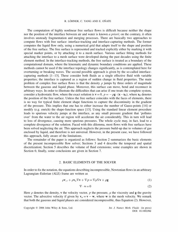
• Advective–diffusive prediction: vn → v∗[ �

�t− �∇�∇

] (v∗ − vn

) + vna · ∇vn + ∇ pn =∇�∇vn + �g (5)

• Pressure correction: pn → pn+1

∇ · vn+1 = 0 (6)



�vn+1 − v∗

�t+ ∇(pn+1 − pn) = 0 (7)

which results in

∇ · 1�

∇(pn+1 − pn) = ∇ · v∗

�t(8)

• Velocity correction: v∗ → vn+1

vn+1 = v∗ − �t

�∇(pn+1 − pn) (9)

At steady state, v∗ = vn = vn+1 and the residuals of the pressure correction vanish, implying thatthe result does not depend on the timestep �t . � denotes the implicitness factor for the viscous terms(� = 1: first-order, fully implicit, � = 0.5: second-order, Crank–Nicholson). One can replace theone-step explicit advective–diffusive predictor by a multistage Runge–Kutta scheme [19], allowingfor higher accuracy in the advection-dominated regions and larger timesteps without a noticeableincrement in CPU cost.

A k-step, time-accurate Runge–Kutta scheme of order k for the advective parts may be writtenas

�vi = �vn + �i��t(−�vi−1

a · ∇vi−1 − ∇ pn + ∇�∇vi−1)

; i = 1, k − 1 (10)

[ �

�t− �∇�∇

](vk − vn) + �vk−1

a · ∇vk−1 + ∇ pn = ∇�∇vk−1 (11)

Here, the �i are the standard Runge–Kutta coefficients �i = 1/(k + 1 − i). As compared to theoriginal scheme given by Equation (5), the k−1 stages of Equation (10) may be seen as a predictor(or replacement) of vn by vk−1. The original right-hand side has not been modified, so that atsteady state vn = vk−1, preserving the requirement that the steady state be independent of thetimestep �t . The factor � denotes the local ratio of the stability limit for explicit timestepping forthe viscous terms versus the timestep chosen. Given that the advective and viscous timestep limitsare proportional to

�ta ≈ h

|v| ; �tv ≈ �h2

�(12)

we immediately obtain

� = �tv�ta

≈ �|v|h�

≈ Reh (13)

or, in its final form:

�=min(1, Reh) (14)

In regions away from boundary layers, this factor is O(1), implying that a high-order Runge–Kutta scheme is recovered. Conversely, for regions where Reh = O(0), the scheme reverts backto the original one (Equation (5)). Projection schemes of this kind (explicit advection with



a variety of schemes, implicit diffusion, pressure-Poisson equation for either the pressure orpressure increments) have been widely used in conjunction with spatial discretizations based onfinite differences [20–23], finite volumes [24], and finite elements [15–19, 25–34].

One complete timestep is then comprised of the following substeps:

• predict velocity (advective–diffusive predictor, Equations (5), (10) and (11));• extrapolate the pressure (imposition of boundary conditions);• update the pressure (Equation (8));• correct the velocity field (Equation (9));• extrapolate the velocity field; and• update the scalar interface indicator.

4. SPATIAL DISCRETIZATION

As stated before, we desire a spatial discretization with unstructured grids in order to:

• Approximate arbitrary domains, and• Perform adaptive refinement in a straightforward manner, i.e. without changes to the solver.

From a numerical point of view, the difficulties in solving Equations (1)–(3) are the usual ones.First-order derivatives are problematic (overshoots, oscillations, instabilities), while second-orderderivatives can be discretized by a straightforward Galerkin approximation. We will first treat theadvection operator and then proceed to the divergence operator. Given that tetrahedral grids solversbased on edge data structures incur a much lower indirect addressing and CPU overhead than thosebased on element data structures [35], only these will be considered.

4.1. The advection operator

It is well known that a straightforward Galerkin approximation of the advection terms will leadto an unstable scheme (recall that on a 1D mesh of elements with constant size, the Galerkinapproximation is simply a central difference scheme). Three ways have emerged to modify(or stabilize) the Galerkin discretization of the advection terms:

• integration along characteristics [36, 37];• Taylor–Galerkin (or streamline diffusion) [26, 38, 39], and• edge-based upwinding [18].

Of these, we only consider the third option here. The Galerkin approximation for the advectionterms yields a right-hand side of the form

r i = Di jFi j = Di j (fi + f j ) (15)

where the fi are the ‘fluxes along edges’

fi = Si jk Fki , Si jk = di jk

Di j, Di j =

√di jk di jk (16)

Fi j = fi + f j , fi = (Si jk vki )vi , f j = (Si jk vkj )v j (17)



and the edge-coefficients are based on the shape-functions Ni as follows:

di jk = 1

2

∫�(Ni

,k Nj − N j

,k Ni ) d� (18)

A consistent numerical flux is given by

Fi j = fi + f j − |vi j |(vi − v j ), vi j = 12 S

i jk (vki + vkj ) (19)

As with all other edge-based upwind fluxes, this first-order scheme can be improved by reducingthe difference vi − v j through (limited) extrapolation to the edge centre [35]. The same scheme isused for the transport equation that describes the propagation of the VOF fraction, PC or distanceto the free surface given by Equation (3).

4.2. The divergence operator

A persistent difficulty with incompressible flow solvers has been the derivation of a stable schemefor the divergence constraint (2). The stability criterion for the divergence constraint is also knownas the Ladyzenskaya–Babuska–Brezzi or LBB condition [40]. The classic way to satisfy the LBBcondition has been to use different functional spaces for the velocity and pressure discretization[41]. Typically, the velocity space has to be richer, containing more degrees of freedom thanthe pressure space. Elements belonging to this class are the p1/p1+bubble mini-element [42],the p1/iso-p1 element [43], and the p1/p2 element [44]. An alternative way to satisfy the LBBcondition is through the use of artificial viscosities [15], ‘stabilization’ [45–47] or a ‘consistentnumerical flux’ (more elegant terms for the same thing). The equivalency of these approaches hasbeen repeatedly demonstrated (e.g. References [15, 35, 42]). The approach taken here is based onconsistent numerical fluxes, as it fits naturally into the edge-based framework. For the divergenceconstraint, the Galerkin approximation along edge i, j is given by

Fi j = fi + f j , fi = Si jk vki , f j = Si jk vkj (20)

A consistent numerical flux may be constructed by adding pressure terms of the form:

Fi j = fi + f j − |�i j |(pi − p j ) (21)

where the eigenvalue �i j is given by the ratio of the characteristic advective timestep of the edge�t and the characteristic advective length of the edge l:

�i j = �t i j

li j(22)

Higher-order schemes can be derived by reconstruction and limiting, or by substituting the first-order differences of the pressure with third-order differences:

Fi j = fi + f j − |�i j |(pi − p j + li j

2(∇ pi + ∇ p j )

)(23)

This results in a stable, low-diffusion, fourth-order damping for the divergence constraint.



5. VOLUME OF FLUID EXTENSIONS

The extension of a solver for the incompressible Navier–Stokes equations to handle free surfaceflows via the VOF or LS techniques requires a series of extensions which are the subject ofthe present section. Before going on, we remark that both the VOF and LS approaches wereimplemented as part of this effort. Experience indicates that both work well. For VOF, it isimportant to have a monotonicity preserving scheme for �. For LS, it is important to balance thecost and accuracy loss of reinitializations vis a vis propagation. Given that the advection solversused are all monotonicity preserving, and that the VOF option is less CPU-demanding than LS,only the VOF technique is considered in the following. In what follows, we will assume that� is bounded by values for liquid and gas (e.g. 0��1 for VOF, �g��l for PC) and thatthe liquid–gas interface is defined by the average of these extreme values (i.e. �= 0.5 for VOF,� = 0.5 · (�g + �l) for PC, � = 0 for LS).

5.1. Extrapolation of the pressure

The pressure in the gas region needs to be extrapolated in order to obtain the proper velocitiesin the region of the free surface. This extrapolation is performed using a three-step procedure. Inthe first step, the pressures for all points in the gas region are set to (constant) values, either theatmospheric pressure or, in the case of bubbles, the pressure of the particular bubble. In a secondstep, the gradient of the pressure for the points in the liquid that are close to the liquid–gas interfaceare extrapolated from the points inside the liquid region (see Figure 1). This step is required asthe pressure gradient for these points cannot be computed properly from the data given. Using thisinformation (i.e. pressure and gradient of pressure), the pressure for the points in the gas that areclose to the liquid–gas interface are computed.

5.2. Extrapolation of the velocity

The velocity in the gas region needs to be extrapolated properly in order to propagate accuratelythe free surface. This extrapolation is started by initializing all velocities in the gas region tov= 0. Then, for each subsequent layer of points in the gas region where velocities have not been

p

p

p=pgp=pg

p=pg

p

p

Liquid

Interface

Gas

p

pp

p

p

p

Figure 1. Extrapolation of the pressure.



Interface

v

v

v

Layer 1

Layer 2

Gas

Liquid

v

Figure 2. Extrapolation of the velocity.

extrapolated (unknown values), an average of the velocities of the surrounding points with knownvalues is taken (see Figure 2).

5.3. Keeping interfaces sharp

The VOF and PC options propagate Heavyside functions through an Eulerian mesh. The‘sharpness’ of such profiles requires the use of monotonicity preserving schemes for advection,such as total variation diminishing (TVD) or flux-corrected transport (FCT) techniques [35]. Levelset methods propagate a linear function, numerically a much simpler problem. Regardless of thetechnique used, one finds that shear and vortical flowfields will tend to smooth and distort �. For-tunately, both TVD and FCT algorithms allow for limiters that keep the solution monotonic whileenhancing the sharpness of the solution. For the TVD schemes Roe’s Super-B limiter [48] producesthe desired effect. For FCT one increases the anti-diffusion by a small fraction (e.g. c= 1.01). Thelimiting procedure keeps the solution monotonic, while the increased anti-diffusion steepens � asmuch as possible on a mesh. With these schemes, the discontinuity in � is captured within 1–2gridpoints for all times. For LS the distance-function � must be reinitialized periodically so thatit truly represents the distance to the liquid–gas interface.

5.4. Imposition of constant mass

Experience indicates that the amount of liquid mass (as measured by the region where the VOFindicator is larger than a cut-off value) does not remain constant for typical runs. The reasons forthis loss or gain of mass are manifold: loss of steepness in the interface region, inexact divergenceof the velocity field, boundary velocities, etc. This lack of exact conservation of liquid mass hasbeen reported repeatedly in the literature [5, 11, 49]. The recourse taken here is the classic one:add/remove mass in the interface region in order to obtain an exact conservation of mass. Atthe end of every timestep, the total amount of fluid mass is compared to the expected value. Theexpected value is determined from the mass at the previous timestep, plus the mass-flux acrossall boundaries during the timestep. The differences in expected and actual mass are typically verysmall (less than 10−4), so that quick convergence is achieved by simply adding and removingmass appropriately. The amount of mass taken/added is made proportional to the absolute value of



the normal velocity of the interface:

vn =∣∣∣∣v · ∇�

|∇�|∣∣∣∣ (24)

In this way, the regions with no movement of the interface remain unaffected by the changes madeto the interface in order to impose strict conservation of mass. The addition and removal of masstypically occurs at points close the liquid–gas interface, where � does not assume extreme values.In some instances, the addition or removal of mass can lead to values of � outside the allowedrange. If this occurs, the value is capped at the extreme value, and further corrections are carriedout at the next iteration.

5.5. Deactivation of air region

Given that the air region is not treated/updated, any CPU spent on it may be considered wasted.Most of the work is spent in loops over the edges (upwind solvers, limiters, gradients, etc.). Giventhat edges have to be grouped in order to avoid memory contention/allow vectorization whenforming right-hand sides [50, 51], this opens a natural way of avoiding unnecessary work: formrelatively small edge-groups that still allow for efficient vectorization, and deactivate groups insteadof individual edges [35]. In this way, the basic loops over edges do not require any changes. Theif-test whether an edge group is active or deactive occurs outside the inner loops over edges,leaving them unaffected. On scalar processors, edges-groups as small as negrp=8 are used.Furthermore, if points and edges are grouped together in such a way that proximity in memorymirrors spatial proximity, most of the edges in air will not incur any CPU penalty.

5.6. Treatment of bubbles

The treatment of bubbles follows the classic assumption that the timescales associated with speedof sound in the bubble are much faster than the timescales of the surrounding fluid. This impliesthat at each instance the pressure in the bubble is (spatially) constant. As long as the bubble isnot in contact with the atmospheric air (see Figure 3), the pressure can be obtained from the

Air

Free Surface

Bubble

Figure 3. Bubble in water.



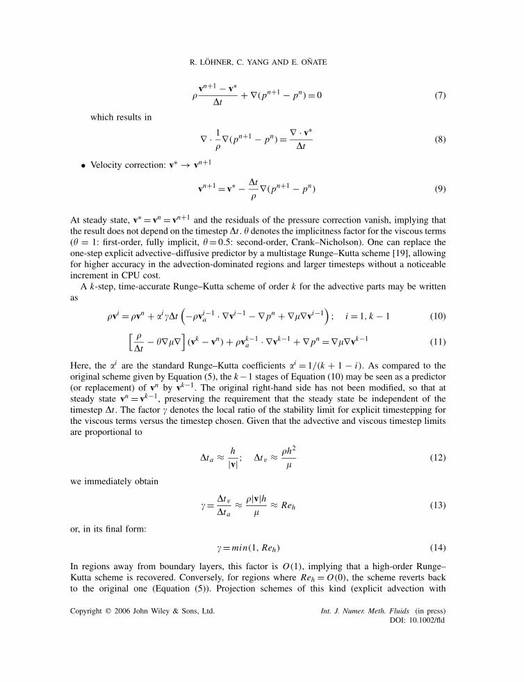
isentropic relation

pbpb0

=(

�b�b0

)�

(25)

where pb, �b denote the pressure and density in the bubble and pb0, �b0 the reference values(e.g. those at the beginning of the simulation). The gas in the bubble is marked by solving a scalaradvection equation of the form given by Equation (3):

b, t + va · ∇b= 0 (26)

where, initially, b= 1.0 denotes the bubble region and b= 0.0 the remainder of the flowfield. Thesame advection schemes and steepening algorithms as used for � as described above are also usedfor b. At the beginning of every timestep the total volume occupied by gas is added. From thisvolume the density is inferred, and the pressure is computed from Equation (25).

At the end of every timestep, a check is performed to see if the bubble has reached contactwith the air. This happens if we have, at a given point: b>0.5 and �>�0.5. Should this be thecase, the neighbour elements of these points that are in air are set to b= 1.0. This increases thevolume occupied by the bubble, thereby reducing the pressure. Over the course of a few timesteps,the pressure in the bubble then reverts to atmospheric pressure, and one observes a rather quickbubble collapse.

5.7. Adaptive refinement

Adaptive mesh refinement is very often used to reduce CPU and memory requirements withoutcompromising the accuracy of the numerical solution. For transient problems with moving disconti-nuities, adaptive mesh refinement has been shown to be an essential ingredient of production codes[52, 53]. For multiphase problems the mesh can be refined automatically close to the liquid–gasinterface. This has been done in the present case by including two additional refinement indicators(on top of the usual ones based on the flow variables). The first one looks at the edges cut bythe liquid–gas interface value of �, and refines the mesh to a certain element size or refinementlevel [54]. The second, more sophisticated indicator, looks at the liquid–gas interface curvature,and refines the mesh only in regions where the element size is deemed insufficient.

6. EXAMPLES

6.1. Breaking dam problem

This is a classic test case for free surface flows. The problem definition is shown inFigure 4(a). This case was run on a coarse mesh with nelem=16562 elements, a fine mesh withnelem=135869 and an adaptively refined mesh (where the coarse mesh was the base mesh)with approximately nelem=30000 elements. The refinement indicator for the latter was thefree surface (see above), and the mesh was adapted every 5 timesteps.

Figure 4(b) shows the discretization for the coarse mesh, and Figures 4(c–f) the developmentof the flowfield and the free surface until the column of water hits the right wall. Note the mesh



14.0

7.0

3.5

10.0ρ=0.9982µ=0.01

1.0

1.5

2.0

2.5

3.0

3.5

4.0

0.0 0.5 1.0 1.5 2.0 2.5 3.0

dim

ensi

onle

ss d

ispl

acem

ent

dimensionless time

Martin/MoyceHansbo

WalhornSauer

KoelkeFEFLO CoarFEFLO Fine

(a) (b)

(c) (d)

(e) (f )

(g)

Figure 4. (a) Breaking dam: problem definition; (b) breaking dam: surface discretization for the coarsemesh; (c–f) breaking dam: flowfield at different times; and (g) breaking dam: horizontal displacement.



adaptation in time. The results obtained for the horizontal location of the free surface alongthe bottom wall are compared to the experimental values of Martin and Moyse [55], as wellas the numerical results obtained by Hansbo [56], Kolke [57] and Walhorn [58] in Figure4(g). The dimensionless time and displacement are given by �= t

√2g/a and � = x/a, where

a is the initial width of the water column. As one can see, the agreement is very good, evenfor the coarse mesh. The difference between the adaptively refined mesh and the fine meshwas almost indistinguishable, and therefore only the results for the fine mesh are shown in thegraph.

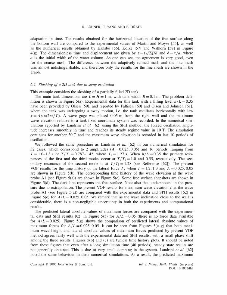
6.2. Sloshing of a 2D tank due to sway excitation

This example considers the sloshing of a partially filled 2D tank.The main tank dimensions are L = H = 1 m, with tank width B = 0.1 m. The problem defi-

nition is shown in Figure 5(a). Experimental data for this tank with a filling level h/L = 0.35have been provided by Olsen [59], and reported by Faltisen [60] and Olsen and Johnsen [61],where the tank was undergoing a sway motion, i.e. the tank oscillates horizontally with lawx = A sin(2t/T ). A wave gage was placed 0.05 m from the right wall and the maximumwave elevation relative to a tank-fixed coordinate system was recorded. In the numerical sim-ulations reported by Landrini et al. [62] using the SPH method, the forced oscillation ampli-tude increases smoothly in time and reaches its steady regime value in 10 T. The simulationcontinues for another 30 T and the maximum wave elevation is recorded in last 10 periods ofoscillation.

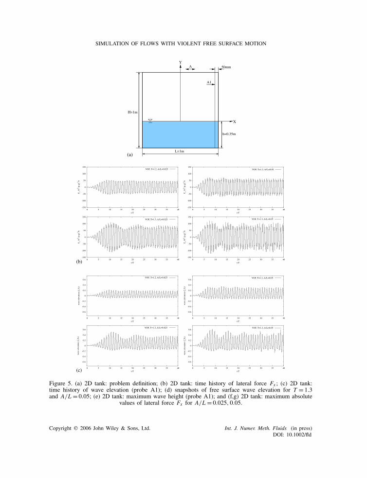
We followed the same procedure as Landrini et al. [62] in our numerical simulation for32 cases, which correspond to 2 amplitudes (A= 0.025, 0.05) and 16 periods, ranging fromT = 1.0–1.8 s or T/T1 = 0.787–1.42, where T1 = 1.27 s. When h/L = 0.35 the primary reso-nances of the first and the third modes occur at T/T1 = 1.0 and 0.55, respectively. The sec-ondary resonance of the second mode is at T/T1 = 1.28 (see Reference [62]). The presentVOF results for the time history of the lateral force Fx when T = 1.2, 1.3 and A= 0.025, 0.05are shown in Figure 5(b). The corresponding time history of the wave elevation at the waveprobe A1 (see Figure 5(a)) are shown in Figure 5(c). Some free surface snapshots are shown inFigure 5(d). The dark line represents the free surface. Note also the ‘undershoots’ in the pres-sure due to extrapolation. The present VOF results for maximum wave elevation at the waveprobe A1 (see Figure 5(a)) are compared with the experimental data and SPH results [62] inFigure 5(e) for A/L = 0.025, 0.05. We remark that as the wave inclination close to the wall isconsiderable, there is a non-negligible uncertainty in both the experiments and computationalresults.

The predicted lateral absolute values of maximum forces are compared with the experimen-tal data and SPH results [62] in Figure 5(f) for A/L = 0.05 (there is no force data availablefor A/L = 0.025). Figure 5(g) shows the comparison of predicted lateral absolute values ofmaximum forces for A/L = 0.025, 0.05. It can be seen from Figures 5(e–g) that both maxi-mum wave height and lateral absolute values of maximum forces predicted by present VOFmethod agrees fairly well with the experimental data and SPH results, with a small phase shiftamong the three results. Figures 5(b) and (c) are typical time history plots. It should be notedfrom these figures that even after a long simulation time (40 periods), steady state results arenot generally obtained. This is due to very small damping in the system. Landrini et al. [62]noted the same behaviour in their numerical simulations. As a result, the predicted maximum



(a)

(b)

(c)

Figure 5. (a) 2D tank: problem definition; (b) 2D tank: time history of lateral force Fx ; (c) 2D tank:time history of wave elevation (probe A1); (d) snapshots of free surface wave elevation for T = 1.3and A/L = 0.05; (e) 2D tank: maximum wave height (probe A1); and (f,g) 2D tank: maximum absolute

values of lateral force Fx for A/L = 0.025, 0.05.



0

0.1

0.2

0.3

0.4

0.5

0.6

0.7

0.7 0.8 0.9 1 1.1 1.2 1.3 1.4 1.5

wav

e he

ight

(ζ

/L)

T/ T

T/ T T/ T

T/ T

VOF, A/L=0.025Exp, A/L=0.025SPH, A/L=0.025

0

0.1

0.2

0.3

0.4

0.5

0.6

0.7

0.7 0.8 0.9 1 1.1 1.2 1.3 1.4 1.5

wav

e he

ight

(ζ

/ L)


0

20

40

60

80

100

120

140

160

180

0.7 0.8 0.9 1 1.1 1.2 1.3 1.4 1.5

F 1

0 /ρ

gL

b


0

20

40

60

80

100

120

140

160

180

0.7 0.8 0.9 1 1.1 1.2 1.3 1.4 1.5

F 1

0 /ρ

gL

b

VOF, A/L=0.050VOF, A/L=0.025

(d)

(e)

(f ) (g)

Figure 5. Continued.



wave elevation and the lateral absolute values of maximum forces plotted in Figure 5(e) areaverage maximum values for the last few periods for the cases when the steady state is notreached.

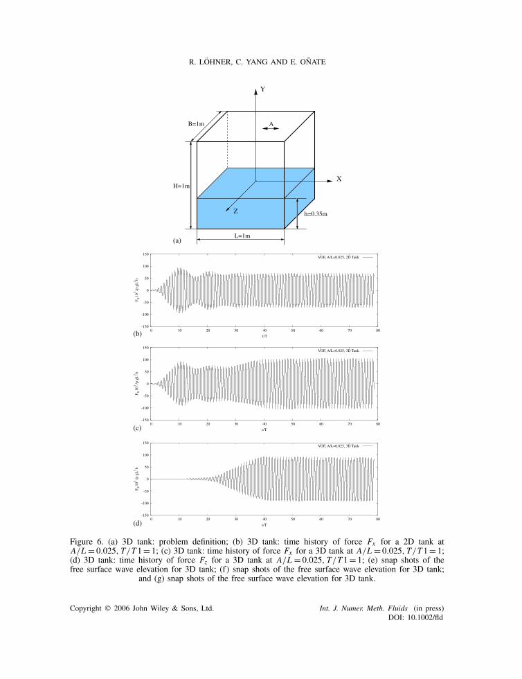
6.3. Sloshing of a 3D tank due to sway excitation

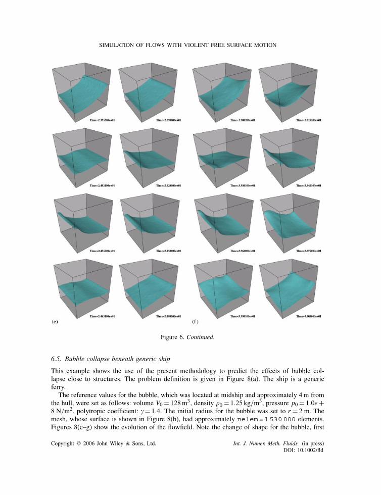
In order to study the 3D effects, the sloshing of a partially filled 3D tank is considered. Themain tank dimensions are L = H = 1 m, with tank width b= 1 m. The problem definition isshown in Figure 6(a). The 3D tank has the same filling level h/L = 0.35 as the 2D tank. The3D tank case is run on a mesh with nelem=561808 elements, and the 2D tank is run on amesh with nelem=54124 elements. The numerical simulations are carried out for both 3Dand 2D tanks, where both tanks are undergoing the same prescribed sway motion given byx = A sin(2 t/T ). The simulations were carried out for A= 0.025 and T = 1.27 (i.e. T/T1 = 1).The forced oscillation amplitude increases smoothly in time and reaches its steady regime valuein 10 T. The simulation continues for another 70 T. In order to show the 3D effects, the forcesare non-dimensionalized with �gL2b for both 2D and 3D tanks. Figures 6(b) and (c) show thetime history of the force Fx (horizontal force in the same direction as the tank moving direction)for both 2D and 3D tanks. Figure 6(d) shows the time history of the force Fz (horizontal forceperpendicular to the tank moving direction) for 3D tank. It is very interesting to observe fromFigures 6(c) and (d) that there are almost no 3D effects for the first 25 oscillating periods. The3D modes start to appear after 25 T, and fully build up at about 40 T. The 3D flow pattern thenremains steady and periodic for the rest of the simulation, which is about 40 more oscillationperiods.

Figures 6(e)–(g) show a sequence of snapshots of the free surface wave elevation for the 3Dtank. For the first set of snapshots (see Figure 6(e)), the flow is still 2D. The 3D flow starts tobuild up in the second set of snapshots (see Figure 6(f)). The flow remains periodic 3D for thelast 40 periods. Figure 6(g) show the typical snapshots of the free surface for the last 40 periods.The 3D effects are clearly shown in these plots.

6.4. Drifting ship

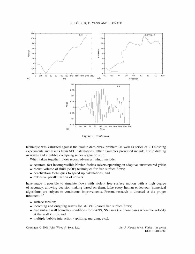
This example shows the use of the present methodology to predict the effects of drift in wavesfor large ships. The problem definition is given in Figure 7(a). The ship is a generic LNG tanker,and is considered rigid. The waves are generated by moving the left wall of the domain. A largeelement size was specified at the far end of the domain in order to dampen the waves. The meshat the ‘wave-maker plane’ is moved using a sinusoidal excitation. The ship is treated as a free,floating object subject to the hydrodynamic forces of the water. The surface nodes of the shipmove according to a 6 DOF integration of the rigid body motion equations. Approximately 30layers of elements close to the ‘wave-maker plane’ and the ship are moved, and the Navier–Stokes/VOF equations are integrated using the arbitrary Lagrangian–Eulerian frame of reference.The LNG tanks are assumed 80% full. This leads to an interesting interaction of the slosh-ing inside the tanks and the drifting ship. The mesh had approximately nelem=2670000elements, and the integration to 3 min of real time took 20 h on a PC (3.2 GHz Intel P4,2 GB RAM, Lunix OS, Intel compiler). Figure 7(b) shows the evolution of the flowfield, andFigures 7(c) and (d) the body motion. Note the change in position for the ship, as well asthe roll.



L=1m

H=1mX

h=0.35m

Y

AB=1m

Z

(a)

(b)

(c)

(d)

Figure 6. (a) 3D tank: problem definition; (b) 3D tank: time history of force Fx for a 2D tank atA/L = 0.025, T/T 1= 1; (c) 3D tank: time history of force Fx for a 3D tank at A/L = 0.025, T/T 1= 1;(d) 3D tank: time history of force Fz for a 3D tank at A/L = 0.025, T/T 1= 1; (e) snap shots of thefree surface wave elevation for 3D tank; (f ) snap shots of the free surface wave elevation for 3D tank;

and (g) snap shots of the free surface wave elevation for 3D tank.




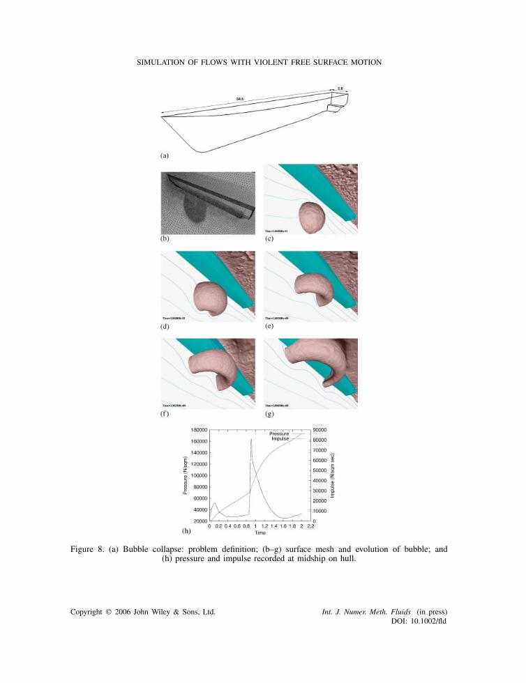
6.5. Bubble collapse beneath generic ship

This example shows the use of the present methodology to predict the effects of bubble col-lapse close to structures. The problem definition is given in Figure 8(a). The ship is a genericferry.

The reference values for the bubble, which was located at midship and approximately 4m fromthe hull, were set as follows: volume V0 = 128m3, density �0 = 1.25 kg/m3, pressure p0 = 1.0e+8 N/m2, polytropic coefficient: � = 1.4. The initial radius for the bubble was set to r = 2 m. Themesh, whose surface is shown in Figure 8(b), had approximately nelem=1530000 elements.Figures 8(c–g) show the evolution of the flowfield. Note the change of shape for the bubble, first




into a torus and subsequently into a rather complex shape. The pressure recorded at midship onthe hull is shown in Figure 8(h).

7. CONCLUSIONS AND OUTLOOK

A volume of fluid (VOF) technique has been developed and coupled with an incompressibleEuler/Navier–Stokes solver operating on adaptive, unstructured grids to simulate the interactionsof extreme waves and 3D structures. The present implementation follows the classic VOF im-plementation for the liquid–gas system, considering only the liquid phase. The velocities andpressure in the gas region near the free surface are obtained via extrapolation algorithms. The VOF



Figure 7. (a) Ship adrift: problem definition; (b) evolution of the free surface; (c–d) position of centreof mass; and (e) roll angle vs time.



-40

-20

0

20

40

60

80

100

120

0 20 40 60 80 100 120 140 160 180 200 220

Pos

ition

Time

x_c

-5

0

5

10

15

20

25

30

35

-40 -20 0 20 40 60 80 100 120

z-P

ositi

on

x-Position

x_c vs z_c

-0.15

-0.1

-0.05

0

0.05

0.1

0.15

0.2

0 20 40 60 80 100 120 140 160 180 200 220

Ang

le

Time

a_x

(c) (d)

(e)


technique was validated against the classic dam-break problem, as well as series of 2D sloshingexperiments and results from SPH calculations. Other examples presented include a ship driftingin waves and a bubble collapsing under a generic ship.

When taken together, these recent advances, which include:

• accurate, fast incompressible Navier–Stokes solvers operating on adaptive, unstructured grids;• robust volume of fluid (VOF) techniques for free surface flows;• deactivation techniques to speed up calculations; and• extensive parallelization of solvers

have made it possible to simulate flows with violent free surface motion with a high degreeof accuracy, allowing decision-making based on them. Like every human endeavour, numericalalgorithms are subject to continuous improvements. Present research is directed at the propertreatment of

• surface tension;• incoming and outgoing waves for 3D VOF-based free surface flows;• free surface wall boundary conditions for RANS, NS cases (i.e. those cases where the velocityat the wall v= 0); and

• multiple bubble interaction (splitting, merging, etc.).



Figure 8. (a) Bubble collapse: problem definition; (b–g) surface mesh and evolution of bubble; and(h) pressure and impulse recorded at midship on hull.



ACKNOWLEDGEMENTS

A considerable part of this work was carried out at the International Center for Numerical Methods inEngineering (CIMNE) of the Universidad Politecnica de Catalunya, Barcelona, Spain. The support forthis visit is gratefully acknowledged.

The authors also wish to thank Mr Andrea Colagrossi of the INSEAN for providing both experimentaldata and numerical results for the sloshing of a 2D tank.

REFERENCES

1. Nichols BD, Hirt CW. Methods for calculating multi-dimensional, transient free surface flows past bodies.Proceedings of the First International Conference on Numerical Ship Hydrodynamics, Gaithersburg, ML, 20–23October 1975.

2. Hirt CW, Nichols BD. Volume of fluid (VOF) method for the dynamics of free boundaries. Journal ofComputational Physics 1981; 39:201–225.

3. Yabe T, Aoki T. A universal solver for hyperbolic equations by cubic-polynomial interpolation. Computer PhysicsCommunications 1991; 66:219–242.

4. Unverdi SO, Tryggvason G. A front tracking method for viscous incompressible flows. Journal of ComputationalPhysics 1992; 100:25–37.

5. Sussman M, Smereka P, Osher S. A levelset approach for computing solutions to incompressible two-phase flow.Journal of Computational Physics 1994; 114:146–159.

6. Yabe T. Universal solver CIP for solid, liquid and gas, Chapter 3. Computational Fluid Dynamics Review, HafezMM, Oshima K (eds). Wiley, 1997.

7. Scardovelli R, Zaleski S. Direct numerical simulation of free-surface and interfacial flow. Annual Review of FluidMechanics 1999; 31:567–603.

8. Chen G, Kharif C. Two-dimensional Navier–Stokes simulation of breaking waves. Physics of Fluids 1999;11(1):121–133.

9. Fekken G, Veldman AEP, Buchner B. Simulation of green water loading using the Navier–Stokes equations.Proceedings of the 7th International Conference on Numerical Ship Hydrodynamics, Nantes, France, 1999.

10. Biausser B, Fraunie P, Grilli S, Marcer R. Numerical analysis of the internal kinematics and dynamics ofthree-dimensional breaking waves on slopes. International Journal of Offshore and Polar Engineering 2004;14(4):247–256.

11. Enright D, Nguyen D, Gibou F, Fedkiw R. Using the particle level set method and a second order accuratepressure boundary condition for free surface flows. Proceedings of the 4th ASME—JSME Joint Fluids EngineeringConference, FEDSM2003-45144, Kawahashi M, Ogut A, Tsuji Y (eds). Honolulu, HI, 2003; 1–6.

12. Huijsmans RHM, van Grosen E. Coupling freak wave effects with green water simulations. Proceedings of the14th ISOPE, Toulon, France, 23–28 May 2004.

13. Coppola-Owen AH, Codina R. Improving Eulerian two-phase flow finite element approximation with discontinuousgradient pressure shape functions. International Journal for Numerical Methods in Fluids 2005.

14. Codina R, Soto O. A numerical model to track two-fluid interfaces based on a stabilized finite element methodand the level set technique. International Journal for Numerical Methods in Fluids 2002; 4:293–301.

15. Lohner R. A fast finite element solver for incompressible flows. AIAA-90-0398, 1990.16. Martin D, Lohner R. An implicit linelet-based solver for incompressible flows. AIAA-92-0668, 1992.17. Ramamurti R, Lohner R. A parallel implicit incompressible flow solver using unstructured meshes. Computers

and Fluids 1996; 5:119–132.18. Lohner R, Yang C, Onate E, Idelssohn S. An unstructured grid-based, parallel free surface solver. Applied

Numerical Mathematics 1999; 31:271–293.19. Lohner R. Multistage explicit advective prediction for projection-type incompressible flow solvers. Journal of

Computational Physics 2004; 195:143–152.20. Kim J, Moin P. Application of a fractional-step method to incompressible Navier–Stokes equations. Journal of

Computational Physics 1985; 59:308–323.21. Bell JB, Colella P, Glaz H. A second-order projection method for the Navier–Stokes equations. Journal of

Computational Physics 1989; 85:257–283.22. Bell JB, Marcus DL. A second-order projection method for variable-density flows. Journal of Computational

Physics 1992; 101(2):334–348.



23. Alessandrini B, Delhommeau G. A multigrid velocity-pressure-free surface elevation fully coupled solver forcalculation of turbulent incompressible flow around a hull. Proceedings of the 21st Symposium on NavalHydrodynamics, Trondheim, Norway, June 1996.

24. Kallinderis Y, Chen A. An incompressible 3-D Navier–Stokes method with adaptive hybrid grids. AIAA-96-0293,1996.

25. Gresho PM, Upson CD, Chan ST, Lee RL. Recent progress in the solution of the time-dependent, three-dimensional, incompressible Navier–Stokes equations. Proceedings of the 4th International Symposium on FiniteElement Methods in Flow Problems, Kawai T (ed.). University of Tokyo Press, 1982; 153–162.

26. Donea J, Giuliani S, Laval H, Quartapelle L. Solution of the unsteady Navier–Stokes equations by a fractionalstep method. Computer Methods in Applied Mechanics and Engineering 1982; 30:53–73.

27. Gresho PM, Chan ST. On the theory of semi-implicit projection methods for viscous incompressible flows andits implementation via a finite element method that introduces a nearly—consistent mass matrix. InternationalJournal for Numerical Methods in Fluids 1990; 11:621–659.

28. Takamura A, Zhu M, Vinteler D. Numerical simulation of pass-by maneuver using ALE technique. JSAE AnnualConference, Spring, Tokyo, May 2001.

29. Eaton E. Aero-acoustics in an automotive HVAC module. American PAM User Conference, Birmingham, Michigan,24–25 October 2001.

30. Karbon KJ, Kumarasamy S. Computational aeroacoustics in automotive design, computational fluid and solidmechanics. Proceedings of the First MIT Conference on Computational Fluid and Solid Mechanics, Boston, June2001; 871–875.

31. Codina R. Pressure stability in fractional step finite element methods for incompressible flows. Journal ofComputational Physics 2002; 170:112–140.

32. Li Y, Kamioka T, Nouzawa T, Nakamura T, Okada Y, Ichikawa N. Verification of aerodynamic noise simulationby modifying automobile front-pillar shape. JSAE 20025351, JSAE Annual Conference, Tokyo, July 2002.

33. Karbon KJ, Singh R. Simulation and design of automobile sunroof buffeting noise control. 8th AIAA-CEASAero-Acoustics Conference, Brenckridge, June 2002.

34. Camelli F, Lohner R, Sandberg WC, Ramamurti R. VLES study of ship stack gas dynamics. AIAA-04-0072,2004.

35. Lohner R. Applied CFD Techniques. Wiley: New York, 2001.36. Huffenus JD, Khaletzky D. A finite element method to solve the Navier–Stokes equations using the method of

characteristics. International Journal for Numerical Methods in Fluids 1984; 4:247–269.37. Gregoire JP, Benque JP, Lasbleiz P, Goussebaile J. 3-D industrial flow calculations by finite element method.

Springer Lecture Notes in Physics 1985; 218:245–249.38. Kelly DW, Nakazawa S, Zienkiewicz OC, Heinrich JC. A note on anisotropic balancing dissipation in finite element

approximation to convection diffusion problems. International Journal for Numerical Methods in Engineering1980; 15:1705–1711.

39. Brooks AN, Hughes TJR. Streamline upwind/Petrov–Galerkin formulations for convection dominated flows withparticular emphasis on the incompressible Navier–Stokes equations. Computer Methods in Applied Mechanicsand Engineering 1982; 32:199–259.

40. Gunzburger MD. Mathematical aspects of finite element methods for incompressible viscous flows. In FiniteElements: Theory and Application, Dwoyer, Hussaini, Voigt (eds). Springer: Berlin, 1987; 124–150.

41. Fortin M, Thomasset F. Mixed finite element methods for incompressible flow problems. Journal of ComputationalPhysics 1979; 31:113–145.

42. Soulaimani A, Fortin M, Ouellet Y, Dhatt G, Bertrand F. Simple continuous pressure elements for two-and three-dimensional incompressible flows. Computer Methods in Applied Mechanics and Engineering 1987;62:47–69.

43. Thomasset F. Implementation of Finite Element Methods for Navier–Stokes Equations. Springer: Berlin, 1981.44. Taylor C, Hood P. A numerical solution of the Navier–Stokes equations using the finite element method.

Computational Fluids 1973; 1:73–100.45. Franca LP, Hughes TJR, Loula AFD, Miranda I. A new family of stable elements for the stokes problem based

on a mixed Galerkin/least-squares finite element formulation. In Proceedings of the 7th International Conferenceon Finite Elements in Flow Problems, Chung TJ, Karr F (eds). Huntsville, AL, 1989; 1067–1074.

46. Tezduyar TE, Shih R, Mittal S, Ray SE. Incompressible flow computations with stabilized bilinear and linearequal-order interpolation velocity-pressure elements. UMSI Report 90, 1990.

47. Franca LP, Frey SL. Stabilized finite element methods: II. The incompressible Navier–Stokes equations. ComputerMethods in Applied Mechanics and Engineering 1992; 99:209–233.



48. Sweby PK. High resolution schemes using flux limiters for hyperbolic conservation laws. SIAM Journal onNumerical Analysis 1984; 21:995–1011.

49. Sussmam M, Puckett E. A coupled level set and volume of fluid method for computing 3D and axisymmetricincompressible two-phase flows. Journal of Computational Physics 2000; 162:301–337.

50. Lohner R. Some useful renumbering strategies for unstructured grids. International Journal for Numerical Methodsin Engineering 1993; 36:3259–3270.

51. Lohner R. Renumbering strategies for unstructured-grid solvers operating on shared-memory, Cache-based parallelmachines. Computer Methods in Applied Mechanics and Engineering 1998; 163:95–109.

52. Baum JD, Luo H, Mestreau E, Lohner R, Pelessone D, Charman C. A coupled CFD/CSD methodology formodeling weapon detonation and fragmentation. AIAA-99-0794, 1999.

53. Lohner R, Yang C, Baum JD, Luo H, Pelessone D, Charman C. The numerical simulation of strongly unsteadyflows with hundreds of moving bodies. International Journal for Numerical Methods in Fluids 1999; 31:113–120.

54. Lohner R, Baum JD. Adaptive H-refinement on 3-D unstructured grids for transient problems. InternationalJournal for Numerical Methods in Fluids 1992; 14:1407–1419.

55. Martin JC, Moyce WJ. An experimental study of the collapse of a liquid column on a rigid horizontal plane.Philosophical Transactions on Royal Society of London, Series A 1952; 244:312–324.

56. Hansbo P. The characteristic streamline diffusion method for the time-dependent incompressible Navier–Stokesequations. Computer Methods in Applied Mechanics and Engineering 1992; 99:171–186.

57. Kolke A. Modellierung und Diskretisierung bewegter Diskontinuitaten in Randgekoppelten Mehrfeldaufgaben.Ph.D. Thesis, Braunschweig, TU, 2005.

58. Walhorn E. Ein Simultanes Berechnungsverfahren fur Fluid-Struktur-Wechselwirkungen mit Finiten Raum-Zeit-Elementen. Ph.D. Thesis, Braunschweig, TU, 2002.

59. Olsen H. Unpublished Sloshing Experiments at the Technical University of Delft. Delft, The Netherlands, 1970.60. Faltisen OM. A nonlinear theory of sloshing in rectangular tanks. Journal of Ship Research 1974; 18/4:224–241.61. Olsen H, Johnsen KR. Nonlinear sloshing in rectangular tanks. A pilot study on the applicability of analytical

models. Det Norske Veritas Report 74-72-S, vol. II, 1975.62. Landrini M, Colagorossi A, Faltisen OM. Sloshing in 2-D flows by the SPH method. Proceedings of the 8th

International Conference on Numerical Ship Hydrodynamics, Busan, Korea, 2003.


Documents

Simulation of flows with violent free surface motion and - Cimne