Embed Size (px)
Citation preview

APPLICATION OF TURBOCHARGERS IN
SPARK IGNITION PASSENGER VEHICLES By
Wallace William Bester
Thesis presented at the University of Stellenbosch in partial fulfilment of the requirements for the degree of
Master of Science in Mechanical Engineering
Department of Mechanical Engineering Stellenbosch University
Private Bag X1, 7602 Matieland South Africa
Supervisor: Dr A. B. Taylor Co‐supervisor: Dr C. Scheffer
April 2006


i
DECLARATION
I, the undersigned, hereby declare that the work contained in this thesis is my
own work and that I have not previously in its entirety or in part submitted it
at any university for a degree.
Signature:……………………………………………..
Date:……………………………………………….…..


ii
ABSTRACT
The quest for higher efficiency of the internal combustion engine will always
be pursued. Increasingly stringent emission regulations are forcing
manufacturers to downsize on engine displacement and increase specific
power. By adding a turbocharger, the airflow through the engine and hence
the specific power can be increased.
The advantages of a small turbocharged engine over a naturally aspirated
(NA) engine of similar power is that it is lighter, having better part load
efficiency when operating at the same load, while producing less emissions.
Component sharing, increased production volume and lower development
costs are further possible advantages that turbocharging could hold for the
manufacturer.
The objective in this study was to determine the accuracy with which a one
dimensional flow simulation package can predict the performance of a NA
and turbocharged engine. The implications of adding a turbocharger to a NA
engine were also investigated.
Different exhaust manifold concepts were evaluated for the turbocharged
engine. A NA engine was turbocharged and its performance was compared
to the simulated results. Simulation predicted the actual NA engine
performance to within 6% and the actual turbocharged engine performance to
within 9% when developing the same boost pressure. Turbocharging
increased the maximum power by 37% and the torque by 48%. 82% of the
maximum torque was available from 2000 rev/min up to 5500 rev/min. The
turbocharged engine could match the fuel efficiency of the NA engine both at
full load and part load. Thus it is justified that a turbocharger can be used to
increase the specific power while still maintaining part load efficiency.
However turbocharging does increase the mechanical loads on the engine
components, the extent of which was quantified.
It was found that one dimensional analysis is a valuable tool for the use in the
application of turbochargers on SI engines.


iii
OPSOMMING
Daar sal altyd gestreef word om die effektiwiteit van binnebrandenjins te
verhoog. Die toenemende streng uitlaatgas regulasies verplig vervaardigers
om enjins se verplasing te verminder, maar terselfdertyd die spesifieke
kraguitset te verhoog. Die toevoeging van ’n turbo aanjaer kan die lugvloei
deur die enjin vermeerder en dienooreenkomstig ook die krag uitset.
Die voordele van ’n klein turbo aangejaagde (TA) enjin teenoor ’n
onaangejaagde (OA) enjin met gelyke werkverrigting is dat die TA enjin ligter
is, beter deellas effektiwiteit het wanner beide by dieselfde las toestand
opereer terwyl dit minder emissies vrystel. Onderdeel deling, verhoogde
produksie volume en laer ontwikkelings koste is moontlike voordele wat
turbo aanjaging vir die vervaardigers kan inhou.
Die doelwit was om die akkuraatheid te bepaal waarmee ’n 1 dimensionele
vloei analise pakket die werkverrigting van ’n OA en TA enjin voorspel kan
word. Die implikasies van die toevoeging van ’n turbo aanjaer op ’n OA enjin
is ook ondersoek.
Verskillende uitlaat spruitstuk konsepte is geëvalueer vir die TA enjin met
behulp van die 1 dimensionele simulasie pakket. ’n OA enjin is omgebou na
’n TA enjin en die gemete werkverrigting is vergelyk met die voorspelde
resultate. Die simulasie het die werkverrigting van die OA enjin met ’n
akkuraatheid van 6% voorspel. Die werkverrigting van die TA enjin is met ‘’n
akkuraatheid van 9% voorspel wanneer dieselfde aanjagings druk ontwikkel
is. Turbo aanjaging het die maksimum drywing verhoog met 37% en die
wringkrag met 48%. 82% van die maksimum wringkrag is beskikbaar vanaf
2000 opm. tot by 5500 opm. Die TA enjin het die brandstof verbruik van die
OA enjin ge ewenaar beide by deel las sowel as vollas. Die turbo aanjaer
verhoog egter die meganiese belasting op die komponente en hierdie toename
is gekwantifiseer.
Dit is bevind dat 1 dimensionele simulasie ’n nuttige hulpmiddel is in die
implementering van turbo aanjaers op vonkontstekings enjins.


iv
ACKNOWLEDGEMENTS
I would like to thank the following people for their involvement in the
completion of this project:
Dr Andrew Taylor, my supervisor, for his guidance and
motivation throughout my studies;
All CAE personnel for their help and contributions, and
especially Gerhard Lourens for his assistance in the laboratory;
Anton van den Berg at SMD for his patience and accuracy in
manufacturing components needed for this project.


v
TABLE OF CONTENTS
DECLARATION ..................................................................................... i
ABSTRACT ............................................................................................. ii
OPSOMMING.......................................................................................iii
ACKNOWLEDGEMENTS.................................................................. iv
TABLE OF CONTENTS ....................................................................... v
LIST OF FIGURES...............................................................................vii
LIST OF TABLES .................................................................................. xi
LIST OF SYMBOLS AND ABBREVIATIONS..............................xii
1. INTRODUCTION............................................................................1
2. PROJECT OBJECTIVES AND OVERVIEW ..............................3
3. LITERATURE REVIEW..................................................................7
3.1. Supercharging.............................................................................................7
3.2. Turbocharging ............................................................................................8
3.2.1. Turbocharger Theory........................................................................10
3.2.2. Turbocharging CI or SI engines ......................................................16
3.2.3. Energy Available in the Exhaust Gas.............................................18
3.2.4. Constant Pressure Turbocharging..................................................20
3.2.5. Pulse Turbocharging ........................................................................22
3.2.6. Pulse Converters in Turbocharger Applications..........................26
3.3. Engine Management Systems................................................................28
3.3.1. Electronic Throttle Control ..............................................................29
3.3.2. Torque Based Engine Management ...............................................29
3.3.3. Boost Control .....................................................................................31
3.4. Engine Performance Simulation ...........................................................33
3.4.1. Flow Modelling .................................................................................34
3.4.2. Combustion Modelling ....................................................................35
3.4.3. Modelling of Compressors and Turbines......................................37
4. ENGINE SIMULATION...............................................................40
4.1. Engine Simulation Model – 1.6 litre Ford Rocam..............................40
4.2. Engine Optimisation ...............................................................................41
4.2.1. Modelling Strategy for Wastegate Control ...................................43
4.2.2. Exhaust Manifold Simulation..........................................................45
4.2.3. Valve Timing Optimisation .............................................................46
4.3. Exhaust Manifold Concept Evaluation................................................53

vi
5. EXPERIMENTAL APPARATUS.................................................58
5.1. Exhaust Manifold Design.......................................................................58
5.1.1. Pulse interference..............................................................................60
5.1.2. Exhaust Manifold: Concept 1 ..........................................................61
5.1.3. Exhaust Manifold: Concept 2 ..........................................................64
5.2. Intake Piping Design ..............................................................................64
5.2.1. Pre Compressor Pipe........................................................................65
5.2.2. Post Compressor Pipe ......................................................................66
5.3. Variable Wastegate Actuator Design ...................................................67
5.4. Oil Feed and Return lines ......................................................................70
5.5. Fuel System Upgrade ..............................................................................72
5.6. Exhaust System Upgrade ........................................................................73
5.7. Experimental Set up ................................................................................73
5.7.1. Combustion Analysis .......................................................................74
5.7.2. Power Correction ..............................................................................77
5.7.3. Exhaust Gas Measurement ..............................................................78
5.7.4. Engine Calibration ............................................................................81
6. RESEARCH RESULTS..................................................................82
6.1. NA Results: Simulation versus Experiments .....................................82
6.2. Turbocharged Results: Simulation versus Experiments ..................90
6.3. Comparison of the NA and Turbocharged Results.........................101
6.3.1. Comparison of Turbocharged Boost Settings .............................101
6.3.2. Force Analysis .................................................................................105
6.3.3. Energy Balance ................................................................................111
6.3.4. Performance Comparison ..............................................................116
6.3.5. Part load Comparison ....................................................................129
7. CONCLUSION.............................................................................137
8. RECOMMENDATIONS ............................................................140
9. REFERENCES ...............................................................................142
APPENDIX A OPTIMISATION ALGORITHMS .....................145
A.1. Nelder Mead Algorithm.......................................................................145
A.2. Initial Value Scaling for Optimisation..............................................146
APPENDIX B TURBOCHARGER OIL FLOW...........................147
APPENDIX C POWER CORRECTION FACTORS...................148
APPENDIX D FORCE ANALYSIS ...............................................149

vii
LIST OF FIGURES
Figure 2 1 Engine Output Target.............................................................................4
Figure 3 1 Automotive Turbocharger (Venter, 1999) ............................................8
Figure 3 2 Components of a Radial Compressor (Sayers, 1990) ........................11
Figure 3 3 h s Diagram for a Radial Compressor (Watson & Janota, 1984) .....13
Figure 3 4 Components of a Radial Turbine (Watson & Janota, 1984) .............15
Figure 3 5 h s diagram for a radial turbine (Watson & Janota, 1984)................15
Figure 3 6 Naturally Aspirated Ideal Limited Pressure Cycle (Watson &
Janota, 1984) .......................................................................................................18
Figure 3 7 Turbocharged Ideal Pressure Limited Cycle (Watson & Janota,
1984) ....................................................................................................................19
Figure 3 8 Schematic of Birmann pulse converter (Watson & Janota, 1984) ....26
Figure 3 9 Exhaust manifold with pulse converter (Watson & Janota, 1984) ..28
Figure 3 10 Components of ME7 (Gerhardt et al., 1998)......................................30Figure 3 11 Conventional Boost Control Layout (Audi AG, 1998)....................32
Figure 3 12 Typical Electronic Boost Control Layout (Audi AG, 1998)............32
Figure 3 13 3 way Solenoid Valve (Normally open) ...........................................33
Figure 3 14 Wiebe Combustion Curve Shape.......................................................36
Figure 3 15 Wiebe Cumulative Combustion Curve Shape.................................37
Figure 4 1 Simulation model: Ford RSI Turbo......................................................41
Figure 4 2 Measured Rack Travel and Calculated Wastegate Area versus
Boost Pressure ...................................................................................................43
Figure 4 3 Wastegate Area Calculation .................................................................44
Figure 4 4 Simulation Model of Exhaust Manifold: Concept 1..........................45
Figure 4 5 Simulation Model of Exhaust Manifold: Concept 2..........................46
Figure 4 6 Effect of Optimised Valve and Wastegate Settings on Torque........52
Figure 4 7 Exhaust Concept Evaluation: Wastegate Area ..................................54
Figure 4 8 Exhaust Concept Evaluation: Torque..................................................54
Figure 4 9 Exhaust Concept Evaluation: Volumetric Efficiency ........................55
Figure 4 10 Exhaust Concept Evaluation: Airflow...............................................55
Figure 4 11 Exhaust Concept Evaluation: Average Residual Mass...................56
Figure 5 1 Positioning Rig .......................................................................................59
Figure 5 2 Four cylinder engine s valve timing (firing order 1 3 4 2) ..............60
Figure 5 3 Exhaust manifold: Concept 1, CAD model ........................................61
Figure 5 4 Exhaust Manifold Force Diagram........................................................63
Figure 5 5 Exhaust Manifold: Concept 2, CAD model ........................................64
Figure 5 6 Pre Compressor Pipe.............................................................................65
Figure 5 7 Guide Vanes in a Sharp Bend...............................................................66
Figure 5 8 Post Compressor Pipe ...........................................................................67

viii
Figure 5 9 Variable Wastegate Actuator................................................................68
Figure 5 10 VWA Diaphragm Test .........................................................................69
Figure 5 11 Oil Return Schematic ...........................................................................71
Figure 5 12 LogP LogV of motored test ................................................................75
Figure 5 13 Normalised Cumulative Heat Release (NA engine, WOT at
4000 rev/min) .....................................................................................................77
Figure 5 14 Thermocouple Set up (Ricardo, 2002)...............................................78
Figure 5 15 Exhaust Port versus Downstream Temperatures............................80
Figure 6 1 NA Simulation vs Experiment: Torque ..............................................83
Figure 6 2 NA Simulation vs Experiment: Volumetric Efficiency.....................84
Figure 6 3 NA Simulation vs Experiment: Airflow .............................................84
Figure 6 4 NA Simulation vs Experiment: Maximum Combustion Pressure..85
Figure 6 5 NA Simulation vs Experiment: Motored in cylinder Pressure
(1500 rev/min)....................................................................................................86
Figure 6 6 NA Simulation vs Experiment: Exhaust Backpressure ....................87
Figure 6 7 NA Simulation vs Experiment: Specific Fuel Consumption............88
Figure 6 8 NA Simulation vs Experiment: Manifold Absolute Pressure..........88
Figure 6 9 NA Simulation vs Experiment: Intake Manifold Air Temperature 89
Figure 6 10 Turbocharged Simulation versus Experiment: Torque ..................91
Figure 6 11 Turbocharged Simulation versus Experiment: Absolute Boost
Pressure ..............................................................................................................91
Figure 6 12 Turbocharged Simulation vs Experiment: Volumetric Efficiency 92
Figure 6 13 Turbocharged Simulation versus Experiment: Airflow .................93
Figure 6 14 Turbocharged Simulation versus Experiment: Max. Combustion
Pressure ..............................................................................................................94
Figure 6 15 Turbocharged Simulation versus Experiment: SFC........................95
Figure 6 16 Turbocharged Simulation versus Experiment: MAP......................95
Figure 6 17 Turbocharged Simulation versus Experiment: Intake Manifold Air
Temperature ......................................................................................................96
Figure 6 18 Turbocharged Simulation versus Experiment: Compressor Outlet
Temperature ......................................................................................................97
Figure 6 19 Turbocharged Simulation versus Experiment: Wastegate Area ...98
Figure 6 20 Turbocharged Simulation versus Experiment: Wastegate Area as
function of mass flow .......................................................................................99
Figure 6 21 Turbocharged Simulation versus Experiment: Turbine Pressure
Ratio ....................................................................................................................99
Figure 6 22 Turbocharged Simulation versus Experiment: Turbine Inlet
Temperature ....................................................................................................100
Figure 6 23 Turbocharged Boost Settings: Boost Pressure................................102
Figure 6 24 Turbocharged Boost Settings: Lambda ...........................................103
Figure 6 25 Turbocharged Boost Settings: Ignition Timing..............................103

ix
Figure 6 26 Turbocharged Boost Settings: Compressor Operating Points .....104
Figure 6 27 Turbocharged Boost Settings: Torque.............................................105
Figure 6 28 Piston Velocity and Acceleration Correlation................................106
Figure 6 29 Small End Bearing Force Comparison: Analytical versus
Simulation ........................................................................................................107
Figure 6 30 Big End Bearing Force Comparison: Analytical versus Simulation
............................................................................................................................107
Figure 6 31 Analytically Determined Bearing Forces........................................108
Figure 6 32 NA versus Turbocharged Results: Gas Force on Piston...............109
Figure 6 33 NA versus Turbocharged Results: Small end Bearing Forces.....110
Figure 6 34 NA versus Turbocharged Results: Big end Bearing Forces.........110
Figure 6 35 Extrapolation of Specific Heat..........................................................112
Figure 6 36 NA versus Turbocharged Results: Heat Rejection........................113
Figure 6 37 NA versus Turbocharged Results: Oil Temperature ....................114
Figure 6 38 NA engine: Energy Balance at WOT ...............................................115
Figure 6 39 Turbocharged Engine: Energy Balance at WOT............................115
Figure 6 40 NA Engine Torque .............................................................................116
Figure 6 41 NA versus Turbocharged Results: Torque and Power.................117
Figure 6 42 NA versus Turbocharged Results: Ignition Timing......................118
Figure 6 43 NA versus Turbocharged Results: Lambda ...................................118
Figure 6 44 NA versus Turbocharged Results: SFC...........................................119
Figure 6 45 NA versus Turbocharged Results: MAP and TMAP....................120
Figure 6 46 NA versus Turbocharged Results: Wastegate Area......................120
Figure 6 47 NA versus Turbocharged Results: Intake Manifold Air Density121
Figure 6 48 NA versus Turbocharged Results: Ambient and Intake Manifold
Air Temperature..............................................................................................122
Figure 6 49 NA versus Turbocharged Results: Airflow....................................122
Figure 6 50 NA versus Turbocharged Results: Volumetric Efficiency ...........123
Figure 6 51 NA versus Turbocharged Results: Exhaust Manifold Pressure..123
Figure 6 52 NA versus Turbocharged Results: Pressure Difference (Intake
Manifold Exhaust Manifold).......................................................................124
Figure 6 53 NA versus Turbocharged Results: Exhaust Backpressure...........125
Figure 6 54 NA versus Turbocharged Results: Exhaust Manifold Temperature
............................................................................................................................126
Figure 6 55 NA versus Turbocharged Results: Fuel consumption vs Power
Output...............................................................................................................127
Figure 6 56 NA versus Turbocharged Results: Spark Advance and Lambda127
Figure 6 57 NA versus Turbocharged Results: Burn Duration........................128
Figure 6 58 NA versus Turbocharged Results: 50% Burn Point ......................128
Figure 6 59 NA versus Turbocharged Results: Maximum Combustion
Pressure ............................................................................................................129

x
Figure 6 60 NA versus Turbocharged Results: Part load SFC .........................130
Figure 6 61 NA versus Turbocharged Results: Part load Spark Advance .....131
Figure 6 62 NA versus Turbocharged Results: Part load Lambda..................131
Figure 6 63 NA versus Turbocharged Results: Part load Energy Balance at
2500 rev/min ....................................................................................................133
Figure 6 64 NA versus Turbocharged Results: Part load Fuel Flow...............133
Figure 6 65 Required Engine Power ....................................................................134
Figure 6 66 2.0L NA versus Turbocharged SFC at 4000 rev/min.....................135
Figure 6 67 2.0L NA versus Turbocharged SFC at 2500 rev/min.....................136
Figure B 1 K03 Oil Flow Specification (Kühnle, Kopp, Kausch, 1994)............147
Figure D 1 Piston Crank: Free Body Diagram....................................................149

xi
LIST OF TABLES
Table 2 1 Test Engine Specifications ........................................................................3
Table 4 1 Initial Values for Full Factorial Valve Optimisation...........................49
Table 4 2 Full Factorial Results ...............................................................................49
Table 4 3 Simplex Optimisation Results (30 iterations).......................................52
Table 5 1 Material Properties of Mild Steel at High Temperatures (British Iron
and Steel Research Association Metallurgy, 1953).......................................62
Table 6 1 Estimated Fuel Saving...........................................................................136
Table C 1 ECE Standard Reference Conditions .................................................148

xii
LIST OF SYMBOLS AND ABBREVIATIONS
AFR Air Fuel Ratio
ATDC After Top Dead Centre
BDC Bottom Dead Centre
BMEP Brake Mean Effective Pressure
CA Crank Angle
CAD Computer aided Design
CFD Computational Fluid Dynamics
CI Compression Ignition
CR Compression Ratio
ECU Electronic Control Unit
EGR Exhaust Gas Recirculation
EMS Engine Management System
ETA Engine Test Automation
ETC Electronic Throttle Control
EVC Exhaust Valve Closure
EVO Exhaust Valve Opening
ID Inside Diameter
IVC Intake Valve Closure
IVO Intake Valve Opening
KLSA Knock Limited Spark Advance
MAP Manifold Absolute Pressure
MBT Most Beneficial Timing
NA Naturally Aspirated
OD Outside Diameter
OEM Original Equipment Manufacturer
PLC Programmable Logic Controller
SFC Specific Fuel Consumption
SI Spark Ignition
TDC Top Dead Centre
VWA Variable Wastegate Actuator
WOT Wide Open Throttle

1
1. INTRODUCTION
Turbocharged spark ignition (SI) engines have been around since the 1970s,
but their popularity outside the motorsport sector has been small until the
recent advances in engine control. The lack of popularity could partly be due
to the drivability issues associated with early turbocharged engines. The
engine’s response to a sudden increase in driver’s demand was delayed due
to turbocharger lag. The lag was then usually followed by a rapid increase of
power which resulted in loss of traction and possible loss of control over the
car. The advances and developments made in the electronic control and
management of internal combustion engines made it possible to overcome
most of these drivability limitations. Passenger vehicles with turbocharged SI
engines are now becoming more common. Audi, Volvo and VW all offer
different passenger vehicle models with turbocharged SI engines. In the
performance sector Mitsubishi, Porsche, and Subaru offer turbocharged
engines whereas Mercedes offers supercharged and turbocharged engines. In
the quest for more efficient engines, turbocharged engines will most probably
increase in popularity.
The operating principle of a turbocharger is to use energy recovered from the
exhaust gases to force more air into the combustion chamber. This increases
the amount of oxygen in the combustion chamber and hence more fuel can be
burned. If more fuel can be burned, more power can be produced. Therefore
a turbocharged engine can produce more power than a similar size NA
engine. It is claimed that the displacement of a turbocharged engine can be
reduced by up to 40% relative to a NA engine, without compromising power
output. Thus the turbocharged engine could be smaller, lighter and more
fuel efficient as well as produce less emissions. Therefore this is an attractive
option for manufacturers who need to lower their fleet average fuel
consumption, but also for those who must meet emission standards without
compromising performance.
Engine simulation and performance prediction are playing an increasingly
important role in engine development. With engine simulation and
performance prediction much iteration in the development phase can now be
done in simulation, which not only costs less than actual testing but also leads
to faster development times. There are a number of engine simulation
packages available on the market today ranging from packages to simulate
combustion, engine and driveline dynamics, control systems, cooling system
and the valve train, to packages which combine some or all the above into
one.

2
If a one dimensional (1 D) flow simulation could be used to replicate and
predict the complicated three dimensional (3 D) flow found in reality, it
would significantly reduce the computation time. The simpler a simulation
package, the faster it would yield results. Shortening simulation time would
enable more iteration in a specific time frame, enabling a higher level of
optimisation and in the end, a better product. Simplifying the simulation,
certain assumptions must be made, causing inaccuracies. Certain processes in
the internal combustion engine such as flow through a compressor or turbine
are difficult to predict with 1 D simulation only. Thus complex 3 D
computational fluid dynamics (CFD) may be necessary to accurately simulate
the reality. By using 3 D CFD only for certain complex processes rather than
for the whole engine model, it would be possible to retain a high degree of
accuracy while not compromising excessively on computation time.
The research questions that are addressed in this project are firstly to ascertain
what the implications would be of adding a turbocharger to a NA engine and,
secondly, to determine whether the performance of a turbocharged engine
can be predicted accurately by using 1 D flow simulation.

3
2. PROJECT OBJECTIVES ANDOVERVIEW
The objective of the project is to address the following two research questions:
What is the implication of adding a turbocharger to a NA engine;
Can 1 D simulation predict the performance of a turbocharged engine
accurately?
In order to address the above questions, a standard NA engine was converted
to a turbocharged engine and a simulation model of each engine was used for
comparative purposes. A 1.6 litre Ford Rocam engine was chosen for the
project. The maximum power output target was set as 100 kW and a torque
curve as flat as possible for a wide as possible engine speed range. The target
speed range was set as 2000 rev/min up to 5000 rev/min. The engine
specifications and output targets are represented in Table 2 1 and Figure 2 1.
Table 2 1 Test Engine Specifications
Specification: Standard Target
Engine Size [cc] 1594
No. of Cylinders 4
Valves Per Cylinder 2
Compression Ratio 9.48
Bore x Stroke [mm] 82 x 75.48
Max Power [kW] 70 100
Engine Speed @ Max Power
[rev/min]5500
Max. Torque [N m] 137 174
Engine Speed @ Max Torque
[rev/min]2500 2000 5000
Fuel Injection Yes
Fuel Injectors BOSCH 110 g/min BOSCH 160 g/min
Fuel Pressure Regulator BOSCH 2.7 bar BOSCH 3.0 bar
Turbocharger No Yes
Intercooler No
Fuel Octane 95 102.6
Exhaust Manifold STD Cast iron Custom
Exhaust System STD (35 mm ID) Custom (51 mm ID)

4
100.0
120.0
140.0
160.0
180.0
200.0
1000 2000 3000 4000 5000 6000
Engine Speed [rev/min]
Torque[N.m]
0.0
20.0
40.0
60.0
80.0
100.0
Power[kW]
Std. Torque Target Torque Std. Power Target Power
Figure 2 1 Engine Output Target
In order to minimise cost and time, the modifications to the engine were
limited. The complete package was also required to fit in the original car’s
engine bay without any modifications to it. This posed a very challenging
packaging exercise since the transversely mounted engine is of the cross flow
type with the exhaust side of the engine close to the firewall.
The modifications included the design and manufacture of an exhaust
manifold to accommodate the turbocharger. Oil and water were supplied to
the turbocharger and pipes were made to connect the air filter to the
compressor and the compressor to the intake manifold. Due to the increased
airflow, the exhaust had to be replaced by a larger diameter free flow exhaust
to keep the exhaust backpressure within reasonable limits. The standard fuel
injectors were replaced with injectors that would be capable to supply the
increased amount of fuel. The fuel pressure regulator was also changed since
the higher flow injectors required a higher fuel pressure.

5
The intake manifold pressure sensor had to be replaced with a sensor that
would be able to measure pressures above atmospheric pressure. A knock
sensor was added to the engine control unit (ECU) to enable it to retard the
ignition timing in the event of knock. High octane fuel would be used during
testing to reduce the likelihood that knock would occur. The time frame and
budget of the project did not allow for engine failure, thus the use of high
octane fuel was a precautionary measure and not a technical requirement.
The fuelling and timing maps of the ECU were adjusted for maximum
performance at full load. At part load the air fuel ratio was kept the same for
both engines as far as possible (limited by exhaust port temperature), but the
ignition timing was optimised for maximum power output.
The first limitation on engine change was that the compression ratio (CR) of
the engine would not be reduced. It was not envisaged that high boost
pressures would be needed to develop the target output, thus reducing the
CR was not a requirement. Knock would have been a limitation, but by using
the high octane fuel this should be overcome. Reducing CR severely impairs
the efficiency of the engine. Since the aim is to improve engine efficiency,
reducing the CR would contradict the initial intention.
The second limitation was that the valve timing would not be altered. The
result would be non optimal valve timing for the turbocharged engine. The
valve timing is a critical part of the gas exchange mechanism and directly
influences the breathing characteristics of an engine. Optimising the valve
timing could benefit low end torque or high end power, or a compromise
between these two extremes. Developing camshafts and cam profiles is a
science outside the scope of this project. Valve timing optimisation was done
with the simulation in order to demonstrate its advantage.
Thirdly an intercooler would not be used. An intercooler would have a two
fold benefit. It would reduce the intake charge temperature, reducing the
chances of knock and by lowering the temperature it would effectively
increase the density of the air, while using the same boost pressure. Since
high boost pressure would not be required, an intercooler would add
unnecessary cost and complexity to the system. Due to the space limitations
on passenger vehicles, packaging of the intercooler would also pose a very
challenging exercise.

6
The fourth limitation was that only mechanical boost control would be
utilised. This is a major simplification since the mechanical wastegate
responds directly to the boost pressure. Using electronic boost control would
further aid the ability to develop a flat torque curve but the complexity and
time needed to implement such a system would be beyond the scope of this
project. However a mechanical wastegate actuator was developed which
would facilitate independent adjustment of the spring stiffness and the preset
compression of the spring.
This concludes the objectives and overview and defines the framework in
which this project was executed.

7
3. LITERATURE REVIEW
This project was concerned with the turbocharging of a four stroke petrol
engine. Turbocharged four stroke diesel engines will also be discussed briefly
and differences will be highlighted. The discussion, however, omits two
stroke engines due to their different gas exchange processes.
3.1. Supercharging
Supercharging can be defined as the introduction of air (or air/fuel mixture)
into an engine cylinder at a density greater than ambient density. This allows
a proportional increase in the fuel that can be burned and hence raises the
potential power output. The principal objective of supercharging is to
increase power output, not to improve efficiency, although efficiency may
benefit.
Various methods of supercharging are available. These methods can be
classified into two categories. The first category uses a compressor driven by
the engine output shaft to compress the air to a density greater than ambient
density. The compressor can be any positive displacement pump such as a
Roots type blower, a centrifugal compressor or a vane type blower. The
speed of the supercharger is proportional to the engine speed, thus at low
engine speeds the centrifugal compressor might be ineffective because the
output pressure varies approximately as the square of the impeller speed.
The second category, known as turbocharging, uses the energy available in
the exhaust gas to compress the charged air (or air/fuel mixture). The energy
is recovered by expanding the high pressure exhaust gas in a turbine. This
energy is then used to drive the compressor. In big diesel engines axial
turbines and compressors may be used, while radial compressors and
turbines are more common in medium size and small engines.
Turbocharging will be discussed in more detail in the next section.
The main advantage of turbocharging as opposed to supercharging is that
turbocharging uses the energy in the hot exhaust gas that would have been
lost. Supercharging uses power from the engine’s crankshaft and thus less
power is available for propulsion.

8
3.2. Turbocharging
The author acknowledges that the basis of the theory represented in this
section was extracted from Watson and Janota (1984) and Sayers (1990).
The exhaust driven turbocharger was invented by a Swiss engineer named
Buchi, who fitted his creation to a diesel engine back in 1909. However, he
only achieved success many years later (around 1925). It took a long time for
turbochargers to become established, but it is now recognised that their
characteristics are particularly suited to the diesel engine, the reason being
that only air is compressed, and no throttling is used. As a result,
turbocharged diesel engines are becoming recognised as suitable, even
desirable, for private cars as well as for commercial vehicles.
A typical turbocharger consists of a radial turbine, which recovers the energy
from the hot exhaust gases. The turbine is coupled to a radial compressor,
which increases the pressure in the intake manifold. Between the two is a
wide supporting bearing, usually in the form of a free floating journal
bearing, because an ordinary roller bearing would not survive the high
rotational speed (up to 250 000 rev/min) of which a small turbine is capable.
Figure 3 1 shows a typical turbocharger used in automotive applications.
Figure 3 1 Automotive Turbocharger (Venter, 1999)

9
There have been concerns that the increased exhaust backpressure caused by
the turbine is a disadvantage, but analysis refutes this statement. When the
exhaust valve first opens, the pressure inside the cylinder is very much higher
than the pressure in the exhaust manifold. As the cylinder pressure drops, a
stage is reached where the ascending piston has to drive out the gases,
because the pressure in the exhaust system is higher due to the turbine. This
higher backpressure could also increase the amount of residual exhaust gas
inside the combustion chamber.
This represents a loss of energy. However, when the inlet valve opens, the
extra pressure created by the compressor supplies extra energy to force the
piston down on the intake stroke, which represents a net gain in energy.
During the period of valve overlap, the extra pressure in the intake manifold
may even help scavenge the residual exhaust gases out of the clearance
volume, representing a further gain in energy. All this presupposes a well
designed system, with the turbocharger being efficient enough to raise the
boost pressure above the exhaust pressure of the engine. Actual temperature
measurements at full power have shown a significant drop in exhaust gas
temperature across the turbine, which is a measure of the energy removed.
This energy would have gone to waste if the turbocharger were not there.
There are currently two ways of utilising the high pressure of the gas inside
the combustion chamber at the moment of valve opening, namely: constant
pressure turbocharging and pulse turbocharging, each of which has its own
merits and will be discussed in later sections (3.2.4 and 3.2.5).
Maximum allowable boost on Compression Ignition (CI) engines depends
only on the mechanical strength of the engine, because they have no knock
limitations. On SI engines the boost pressure is limited by knock (self ignition
of the end gas under high temperature and pressure). Thus, if the boost
pressure is high on SI engines, the CR must be sufficiently low, high octane
fuel must be used or the ignition timing must be retarded. The difference
between CI and SI combustion are discussed in more detail in section 3.2.2.

10
3.2.1. Turbocharger Theory
The operating characteristics of turbomachines such as compressors and
turbines are completely different from those of the reciprocating internal
combustion engine. Thus matching these two completely different machines
to operate together is an optimisation problem with many parameters. The
basic theory of turbomachines will be briefly reviewed to highlight certain
key aspects that must be borne in mind when combining turbomachines with
reciprocating internal combustion engines.
The most common turbocharger assembly used in the automotive industry
consists of a radial compressor coupled to a radial turbine. The bearings are
generally of the plain journal bearing type; however, for racing applications
ceramic ball bearings are being used more frequently. On big engines such as
those used for rail and marine applications, where the operating range is very
narrow and operation is mostly steady state, an axial turbine coupled to a
radial compressor is the most common configuration. Axial turbines are
preferred for their superior efficiency to those of a radial turbine, but a radial
turbine’s operating range is much wider. This makes radial turbines more
suitable for automotive applications, where the operating range is very wide.
Radial compressors also have a much wider operating range and are thus
more widely used than axial compressors in turbocharger applications.
Radial compressors are limited to a pressure ratio of about 3.5, because higher
pressure ratios will cause supersonic flow and cause shockwaves to form at
the compressor inlet. This will cause a rapid deterioration in the compressor
efficiency.
Before discussing the working and characteristics of turbomachines, pressure
and temperature measurements will be revisited and their significance
discussed.
3.2.1.1. Total and Static Pressure and Temperature
The static pressure (P1) of a fluid flowing in a duct is that measured at the
surface of the wall. The total or stagnation pressure (P01) is the pressure thatwill be measured in the stream if the fluid were brought to rest isentropically.
Thus P01 can be related to P1 as in Eq 3 1.)1(
1
01
101T
TPP Eq 3 1

11
Where gamma ( ) represents the polytropic coefficient (ratio of specific heats).
Similarly the static temperature (T1) is the free stream temperature and the
total (or stagnation) temperature (T01) is the temperature that will be
measured if the gas were brought to rest. For a perfect gas it can be shown
that Eq 3 2 holds.
pc
CTT
2
1
1012
1Eq 3 2
Where C1 is the velocity of the gas and cp the specific heat at constant pressure.
3.2.1.2. The Radial Compressor
Figure 3 2 shows the three important parts of a radial compressor: impeller,
diffuser ring and volute casing. In some applications there might be a
diffuser ring included. The diffuser ring is optional and may or may not be
present depending on size, use and cost of the compressor.
The impeller is a solid rotating disc with curved blades standing out axially
from the face of the disc. In most turbocharger applications the blade tips are
left open and the casing of the compressor itself forms the solid outer wall of
the blade passages. In some cases the blade tips may be covered with another
flat disc to give shrouded blades. The advantage of the shrouded blade is that
no leakage can take place from one passage to the next. The disadvantage of
having shrouded blades is extra weight and a more complicated
manufacturing process. In turbocharger applications where very high
rotational speeds are required, the disadvantage of leakage is more than offset
by the reduced weight of the impeller.
Figure 3 2 Components of a Radial Compressor (Sayers, 1990)

12
As the impeller rotates, the fluid (air) that is drawn into the blade passages at
the impeller inlet is accelerated as it is forced radially outwards. In this way,
the static pressure at the outlet radius is much higher than at the inlet radius.
The fluid has a very high velocity at the outer radius of the impeller and, to
recover this kinetic energy by changing it to pressure energy, diffuser blades
mounted on the diffuser ring may be used. The stationary blade passages so
formed have an increasing cross sectional area as the fluid moves through
them, the kinetic energy of the fluid being reduced, while the pressure energy
is further increased. Vaneless diffuser passages may also be utilised.
Finally, the fluid moves from the diffuser blades into the volute casing, which
collects it and conveys it to the compressor outlet. As the fluid moves along
the volute casing, further pressure recovery occurs. Sometimes only the
volute casing exists without the diffuser.
This process can be plotted on an enthalpy versus entropy diagram as shown
in Figure 3 3, so that any departures from isentropic compression can be
shown. Station 01 represents ambient pressure of the air. Acceleration of the
fluid in the inlet causes a pressure drop from P01 to P1 (or P00 to P1 when
considering losses in the inlet), the change in enthalpy being equivalent to the
increase in kinetic energy (C12/2). Isentropic compression to the delivery
stagnation pressure P05s is shown by the vertical line 01 05s. Energy transfer
to the fluid takes place in the impeller and the line 1 2 indicates this process.
The corresponding isentropic process is shown by 1 2s. If the total kinetic
energy of the fluid leaving the impeller (C22/2) were converted to pressure,
isentropically, the delivery pressure would be P02 (point 02). Since the
diffusion process is not accomplished isentropically (2 5), and some kinetic
energy remains at the diffuser exit (velocity C5), the static delivery pressure at
point 5 is P5.

13
Figure 3 3 h s Diagram for a Radial Compressor (Watson & Janota, 1984)
This describes the basic working of a radial compressor. For more detailed
analyses and literature on compressor design the reader is referred to Sayers
(1990) or Watson and Janota (1984).
3.2.1.3. Compressor Efficiency
The efficiency of the radial compressor can be defined as the work required
for ideal adiabatic compression divided by the actual work required to
achieve the same pressure ratio. From the second law of thermodynamics it is
clear that this definition is equivalent to Eq 3 3.
workactual
workisentropicc
Eq 3 3
From the first law of thermodynamics, assuming that the heat transfer rate to
and from the compressor can be neglected as well as the change in potential
energy, Eq 3 3 can be rewritten in the following form:
0102
0102
hh
hh scTT
Eq 3 4
Assuming that air is a perfect gas, thus cp is constant.
0102
0102
TT
TT s
cTTEq 3 5
The expressions are for total to total isentropic efficiency.

14
An evaluation based on Eq 3 5 assumes that all the kinetic energy at the
compressor outlet can be used. This is true in the case of a gas turbine, since
the velocity at the compressor delivery is maintained at the combustion
chamber. However, the compressor of a turbocharger must supply air via a
relatively large inlet manifold to the cylinders. Hence the engine will only
‘feel’ the static pressure at the compressor delivery and is unlikely to benefit
from the kinetic energy at the compressor outlet. Thus a turbocharger
compressor should be designed for high kinetic to potential energy
conversion before the outlet duct.
Since the engine benefits little from the kinetic energy of the air leaving the
compressor, a more realistic definition of the compressor efficiency is based
on static delivery temperature as in Eq 3 6, where TS denotes total to static.
0102
012
TT
TT s
cTSEq 3 6
It is common practice for manufacturers to quote total to total efficiencies for
turbocharger compressors, and quite often those are quoted without declaring
the basis on which the efficiency values are calculated.
3.2.1.4. The Radial Turbine
The radial flow turbine consists of a scroll or inlet casing, a set of inlet nozzles
(sometimes omitted) followed by a short vaneless gap and the turbine wheel
itself (Figure 3 4). Most small turbochargers’ turbines use a vaneless casing;
the nozzle is then in the form of a slot running all the way between the scroll
and turbine wheel. A vaneless casing can be used to improve flow range at
some penalty in peak performance, while also reducing cost. However,
considering the more conventional type with nozzles, the function of the inlet
casing is purely to deliver a uniform flow of inlet gas to the nozzle entries.
The nozzles accelerate the flow, reducing pressure and increasing the kinetic
energy. A short vaneless space prevents the rotor and nozzle blades from
touching and allows wakes coming off the trailing edge of the nozzle blades
to mix out. Energy transfer occurs solely in the impeller, which should be
designed for minimum kinetic energy at the exit.

15
Figure 3 4 Components of a Radial Turbine (Watson & Janota, 1984)
The flow process through the turbine may be plotted on an enthalpy versus
entropy diagram as shown in Figure 3 5. Station 01 refers to stagnation
conditions at the entry to the casing. The gas will already have a significant
velocity (C1), hence the stagnation pressure is P01. The inlet nozzles accelerate
the flow from station 1 to 2. If this process were isentropic, the end point
would be 2s. Energy transfer occurs in the rotor, between station 4 and 5 (4
and 5s if isentropic) down to the exit pressure P5. The stagnation P05 will be
higher than P5 since the exit velocity will remain significant. Station 3 is the
nozzle exit or the nozzle throat, denoted as station 2.
Figure 3 5 h s diagram for a radial turbine (Watson & Janota, 1984)

16
3.2.1.5. Turbine Efficiency
The isentropic efficiency of a turbine may be defined as the actual work
output divided by that obtained from reversible adiabatic (isentropic)
expansion between the same two pressures.
workisentropic
workactualt
Eq 3 7
Assuming a perfect gas (cp = constant) and following the same reasoning as
with compressors, it can be shown that Eq 3 7 can be expressed in terms of
temperatures as in Eq 3 8.
s
tTTTT
TT
0403
0403 Eq 3 8
The total to total efficiency given in Eq 3 8 assumes that the kinetic energy
leaving the turbine exit can be harnessed. In most applications this is not
possible. The energy leaving the turbine exit goes to waste through the
exhaust pipe. Thus a more relevant isentropic efficiency could be based on
the static exit temperature. The total to static isentropic efficiency would be
defined as the actual work output divided by isentropic expansion between
the stagnation inlet and static outlet pressures.
s
tTSTT
TT
403
0403 Eq 3 9
3.2.2. Turbocharging CI or SI engines
Today, turbocharged CI engines are more common than turbocharged SI
engines. There are sound reasons for this, both economic and technical. The
principal reasons stem from the difference between the combustion and
control systems of SI and CI engines. The SI engine use a carburettor or fuel
injection system to mix air and fuel in the inlet manifold so that a
homogeneous mixture is compressed in the cylinder. A spark is used to
control the initiation of combustion, which then spreads throughout the
mixture. It follows that the mixture temperature during compression must be
kept below the self ignition temperature of the fuel.

17
Once combustion has started, it takes time for the flame front to move across
the combustion chamber burning the fuel. During this time, the un burnt
end gas (furthest from the sparkplug) is heated by further compression and
radiation from the flame front. If it reaches the self ignition temperature
before the flame front arrives, a large quantity of mixture may burn very
rapidly, producing severe pressure waves in the combustion chamber. This
situation is commonly referred to as knock and may result in severe cylinder
head and piston damage. Lowering the CR, using fuel with a higher octane
number or retarding the ignition timing are ways to prevent the occurrence of
knock.
In the CI engine cylinder, air alone is compressed. Fuel is injected directly
into the combustion chamber from an injector, only when combustion is
required. This fuel vaporises and mixes with the air, it self ignites and, in
contrast to SI combustion, it follows that in a CI engine the CR must be high
enough for the air temperature during compression to exceed the self ignition
temperature of the fuel. Because injection takes time, only some of the fuel is
in the combustion chamber when ignition starts. Since much of the fuel has
not fully vaporised and mixed with the air, the initial rate of combustion is
not sufficient to initiate destructive pressure waves as in the case of knocking
in a SI engine, and thus does not lead to engine damage.
The maximum CR of the SI engine, but not the CI engine, is therefore limited
by the ignition properties of the fuel. The minimum CR is limited by the
resulting low overall engine efficiency. Turbocharging results in not only a
higher compression pressure, but also a higher temperature.
Unless the CR of a SI engine is reduced the temperature at the end of
compression stroke may be too high and the engine may knock. The engine
may remain knock free under mild boost – but only because there is a
sufficiently safe knock free margin. Thus the potential power output of a
turbocharged SI engine is limited. The CI engine has no such limit and can
therefore use a much higher boost pressure.
SI engines cost substantially less to produce than CI engines of equivalent
power output, primarily as a result of higher operating speeds and cheaper
fuel injection system. The cost of the turbocharger on a CI engine is more
than offset by the reduced engine size required for a specific power output
(with the exception of very small engines). This situation will rarely occur in
the case of a SI engine.

18
3.2.3. Energy Available in the Exhaust Gas
Figure 3 6 shows the ideal limited pressure engine cycle in terms of a
pressure/volume diagram for a naturally aspirated engine. Superimposed is a
line representing isentropic expansion from point 5, at which the exhaust
valve opens, down to the ambient pressure (Pa), which could be obtained by
further expansion if the piston were allowed to move to point 6. The shaded
area 1 5 6 represents the maximum theoretical energy that could be extracted
from the exhaust system; this is called the blow down energy.
Figure 3 6 Naturally Aspirated Ideal Limited Pressure Cycle (Watson &
Janota, 1984)
Consider now the turbocharged engine; the ideal four stroke pressure/volume
diagram would appear as shown in Figure 3 7, where P1 is the turbocharging
or boost pressure and P7 is the exhaust manifold pressure. Process 12 1 is the
induction stroke, during which fresh air at the compressor delivery pressure
enters the cylinder. Process 5 1 13 11 represents the exhaust process. When
the exhaust valve first opens (point 5) some of the gas in the cylinder escapes
to the exhaust manifold expanding along 5 7, if the expansion is isentropic.
Thus the remaining gas in the cylinder is at P7, when the piston moves toward
top dead centre (TDC), displacing the cylinder contents through the exhaust
valve against the backpressure P7. At the end of the exhaust stroke the
cylinder retains a volume (Vcl, clearance volume) of residual combustion
products, which for simplicity can be assumed to remain there. The area 7 8
10 11 will represent the maximum possible energy that could be extracted
during the expulsion stroke, where 7 8 represents isentropic expansion down
to the ambient pressure.

19
Figure 3 7 Turbocharged Ideal Pressure Limited Cycle (Watson & Janota,
1984)
There are two distinct areas in Figure 3 7 representing energy available from
the exhaust gas, the blow down energy (area 5 8 9) and the work done by the
piston (area 13 9 10 11). The maximum possible energy available to drive the
turbocharger turbine will clearly be the sum of these two areas. Although the
energy associated with one area is easier to harness than the other, it is
difficult to devise a system that will harness all the energy. To harness all the
energy; the turbine inlet pressure must rise instantaneously to P5 when the
exhaust valve opens, followed by isentropic expansion of the exhaust gas
through P7 to the ambient pressure (P8=Pa). During the displacement part of
the exhaust process (expulsion stroke) the turbine inlet pressure must be held
at P7. Such a series of processes is impractical.
Consider the simpler process in which a large chamber is fitted between the
engine and the turbine inlet, in order to damp out the pulsating exhaust gas
flow. By forming a restriction to flow, the turbine may maintain its inlet
pressure at P7 for the whole cycle. The available work at the turbine will then
be given by area 7 8 10 11. This is the ideal constant pressure turbocharging
system. Next consider an alternative system, in which a turbine wheel is
placed directly downstream of the engine close to the exhaust valve. If there
were no losses in the port, the gas would expand directly out through the
turbine alone line 5 6 7 8, assuming isentropic expansion. If the turbine area
were sufficiently large, both cylinder and turbine inlet pressures would drop
to P9 before the piston has moved significantly up the bore. Hence the
available energy at the turbine would be given by area 5 8 9. This can be
considered the ideal pulse turbocharging system. The systems commonly
referred to as ‘constant pressure turbocharging’ and ‘pulse turbocharging’ are
based on the above principles, but in practice they differ from the ideal
theoretical cycles.

20
3.2.4. Constant Pressure Turbocharging
With constant pressure turbocharging, the exhaust ports from all cylinders
will be connected to a single exhaust manifold, whose volume will be
sufficiently large to damp down the unsteady flow, caused by the blow down
and expulsion, from each cylinder in turn. Only one turbocharger need be
used, with a single entry. When the exhaust valve of a cylinder opens, the gas
expands down to the (constant) pressure in the exhaust manifold without
doing any useful work. However, not all of the blow down energy is lost.
From the law of conservation of energy, the only energy actually lost between
cylinder and turbine will be due to heat transfer. With a well insulated
manifold, this loss will be very small and can be neglected.
Consider what happens to the exhaust gas leaving the cylinder, expanding
down into the exhaust manifold and then flowing through the turbine. At the
moment of exhaust valve opening, the cylinder pressure will be much higher
than the exhaust manifold pressure. During early stages of valve opening
(when the throat area of the valve is very small) the pressure ratio across the
valve or port will be above the choked value. Hence the gas flow will
accelerate to sonic velocity in the throat followed by a shock wave at the valve
throat and sudden expansion to the exhaust manifold pressure. Due to
turbulent mixing and throttling, no pressure recovery occurs. The stagnation
enthalpy remains unchanged and hence the flow from valve to turbine is
accompanied by an increase in entropy.
As the valve continues to open, the cylinder pressure will fall and flow
through the valve becomes subsonic. The flow will continue to accelerate
through the valve throat and expand to the pressure in the exhaust manifold.
The energy available to do useful work in the turbine is given by the
isentropic enthalpy change across the turbine, whereas the actual energy
recovered is given by the enthalpy change across the turbine. Clearly it is the
lack of recovery of the kinetic energy leaving the valve throat and the
throttling losses that lead to poor exhaust gas energy utilisation with the
constant pressure system.

21
The volume of the exhaust manifold should be sufficient to damp pressure
pulsations down to a low level. Thus the volume required will depend on the
cylinder release pressure and frequency of the exhaust gas pulsations coming
from each cylinder in turn. Pulse amplitude will be a function of engine load,
the timing at which the exhaust valve opens, turbine area and exhaust
manifold volume. Frequency will be dependent on the number of cylinders
and engine speed. The effect of engine speed will be less significant, since the
duration of the exhaust process from each cylinder will be relatively constant
in terms of crank angle, rather than time, and a suitable turbine area will be
chosen at the operating speed and load.
If the exhaust manifold is not sufficiently large, the blow down or first part of
the exhaust pulse from the cylinder will raise the general pressure in the
manifold. If the engine has more than three cylinders, it is inevitable that at
the moment when the blow down pulse from one cylinder arrives in the
manifold, another cylinder is nearing the end of its exhaust process. The
pressure in the latter cylinder will be low, hence any increase in exhaust
manifold pressure will impede or even reverse its exhaust processes. This
will be particularly important where the cylinder has both intake and exhaust
valves partially open (valve overlap) and is relying on a through flow of air
for scavenging of the burnt combustion products.
The constant pressure system has some advantages and disadvantages:
Conditions at turbine entry are steady, thus losses in the turbine that
result from unsteady flow are absent;
A single entry turbine may be used, eliminating ‘end of sector’ losses
(losses associated with flow from one turbine nozzle to another);
Use of a single turbocharger implies a larger turbocharger and larger
machines have higher efficiencies than smaller ones;
A turbine designed for constant pressure operation may have high
degree of reaction, coupled with an exhaust diffuser, bringing
additional gains in efficiency;
From a practical point of view, the exhaust manifold is simple to
construct, but is rather bulky, particularly relative to small engines
with few cylinders;
Transient response of a constant pressure system is poor. Due to the
large volume of gas in the exhaust manifold, the pressure is slow to
rise, resulting in poor engine response and making it unsuitable for
applications with frequent load or speed changes.

22
3.2.5. Pulse Turbocharging
In the practical pulse system an attempt is made to utilise the energy
represented by both the pulse and constant pressure areas of Figure 3 7. The
objective is to make the maximum use of the high pressure and temperature
that exist in the cylinder at the moment of exhaust valve opening, even at the
expense of creating highly unsteady flow through the turbine. In most cases
the benefit from increasing the available energy will more than offset the loss
in turbine efficiency due to unsteady flow.
The constant pressure system was discussed in detail in the previous section.
Now consider a much smaller exhaust manifold. Due to the small volume of
the exhaust manifold, a pressure build up will occur during the exhaust blow
down period. This results from a flow rate of gases entering the manifold
through the exhaust valves exceeding that of gas escaping through the
turbine. At the moment the exhaust valve starts to open, the pressure in the
cylinder will be 6 to 10 times atmospheric pressure, whereas the pressure in
the exhaust manifold will be close to atmospheric. Thus the initial pressure
drop across the valve will be above the critical value at which choking occurs
and the flow will be sonic.
Further expansion of the gas to the exhaust manifold pressure occurs by a
sudden expansion at the valve throat and no pressure recovery occurs due to
turbulent mixing. The stagnation enthalpy remains constant, consequently
the flow from the valve throat is accompanied by an entropy increase. Finally
the gas expands through the turbine to atmospheric pressure, doing useful
work. The out flowing gas from the cylinder loses a very large part of its
available energy in throttling and turbulence after passing the minimum
section of the exhaust valve throat. The throttling losses are very high if the
ratio of valve throat area to manifold cross section area is very small and the
pressure drop across the valve is large, as during the initial stages of exhaust
valve opening.

23
Following further opening of the exhaust valve, the cylinder pressure falls,
but the pressure in the exhaust manifold increases, reducing the throttling
losses across the valve. The pressure drop across the turbine is now much
larger, transferring the available energy to the turbine, which represents a
much larger proportion of the available energy in the cylinder. During the
last portion of valve opening the flow is sub sonic and the throttling loss is
reduced and is equivalent to the kinetic energy at entry to the exhaust
manifold. During the exhaust stroke, the flow process follows approximately
the constant pressure pattern as described in the previous section. At the
exhaust valve, the pressure in the exhaust manifold approaches atmospheric
value.
With pulse operation, a much larger portion of the exhaust energy can be
made available to the turbine by considerably reducing throttling losses
across the exhaust valve. The speed at which the exhaust valve opens to its
full area and the size of the exhaust manifold become important factors as far
as energy utilisation is concerned. If the exhaust valve can be made to open
faster, the throttling losses become smaller during the initial exhaust period.
Furthermore, the smaller the exhaust manifold, the faster the rise in manifold
pressure becomes, contributing to a further reduction in throttling losses in
the early stages of the blow down period. A small exhaust manifold also
causes a much more rapid fall of the manifold pressure towards the end of the
exhaust process improving scavenging and reducing pumping work. This
discussion has thus far focussed on a single cylinder engine connected to a
small exhaust manifold.
The problem becomes more complicated when considering a multi cylinder
engine. Since the turbocharger may be located at one end of the engine,
narrow pipes are used to connect the cylinders to the turbine to keep the size
of the manifold as small as possible. By using narrow pipes the area increase
following the valve throat is greatly reduced, keeping throttling losses to a
minimum. But by using narrow pipes the flow resistance and losses due to
friction become important factors.

24
Consider again a single cylinder engine, connected to a turbine by a long
narrow pipe. Since a large quantity of the exhaust energy becomes available
in the form of pressure waves, which travel along the pipe to the turbine at
sonic velocity, the conditions at the exhaust valve and turbine are not the
same at a given time instant. For simplicity, pressure wave reflections in the
pipe will be ignored. During the first part of the exhaust process, in the
choked region of flow through the valve, the gas is accelerated to sonic
velocity at the throat. Since the contents of the pipe are initially at rest at
atmospheric pressure, sudden expansion takes place across the valve throat.
However, some of the kinetic energy is retained, depending on the ratio of
valve throat area to pipe cross section area.
As the valve opens further the pressure at the exhaust pipe entry rises rapidly.
This is, firstly, because a certain time is required for the acceleration of the
outgoing gases, and secondly, because the gases enter the exhaust pipe from
the cylinder at a higher rate than they are leaving the exhaust pipe at the
turbine end. The rapid pressure rise at the pipe entry is transmitted along the
pipe in the form of a pressure wave, travelling at sonic velocity, and will
arrive at the turbine displaced in time. This phase shift is a function of pipe
length and gas properties (composition, temperature and pressure).
The pressure drop across the valve is noticeably reduced due to the rapid
drop in cylinder pressure and the rise in pipe pressure, and also because the
ratio of valve throat area to pipe area has increased. Both effects considerably
reduce throttling losses. The velocity at the turbine end of the pipe is greater
than the velocity after the valve, due to the arrival of the high pressure wave
at the turbine end. In the sub critical flow region of the blow down period,
the pressure in the exhaust falls at the same time as that in the cylinder. The
velocity at the valve throat is equal to the velocity in the pipe, assuming the
valve throat area is equivalent to the area of the pipe when the valve is fully
open. At the turbine the exhaust gas expands to atmospheric pressure, doing
useful work in the turbine.

25
It has been established that the pulse turbocharging system results in greater
energy availability at the turbine. As the pressure wave travels through the
pipe, it carries a large portion of pressure energy and a small portion of
kinetic energy, which is affected by friction. The gain obtained by using a
narrow exhaust pipe is achieved partly by reducing the throttling losses at the
early stages of the blow down period and partly by preserving kinetic energy.
Thus the small diameter exhaust pipes are essential and, up to a point, the
smaller the better, since this will preserve high gas velocity from the valve to
turbine. However, if the pipes are made too narrow the viscous friction at the
pipe wall will become excessive. The optimum exhaust manifold pipe
diameter will be a compromise, but the cross sectional area should not be
significantly greater than the geometric valve area at full lift.
The actual flow through a pulse exhaust system is highly unsteady and is
affected by pulse reflections from the turbine and closed exhaust valves. It
will be evident that as engine speed changes, the effective time of arrival of a
reflected pulse, in crank angle terms, will vary. Hence the exhaust pipe
length is critical and must be optimised to suit the speed range of the engine.
The interference of reflected pressure waves with the scavenging process is
the most critical aspect of a pulse turbocharging system, particularly on
engines with a very long valve overlap. Due to this phenomenon it is
impossible to connect an engine with more than 3 cylinders to the same
turbine without using a twin entry turbine or introducing losses on the intake
or exhaust processes.
The ideal pulse turbocharging system must have the following two
characteristics. Firstly, the peak of blow down pulse must occur just before
the bottom dead centre (BDC) of that cylinder, followed by a rapid pressure
drop to below boost pressure. The boost pressure must be above exhaust
manifold pressure to aid the scavenging process during valve overlap.
Secondly, the effectiveness of pulse system is governed by the gas exchange
process and overall efficiency of the turbocharger under unsteady flow
conditions. The principal advantage of the pulse system over the constant
pressure system is that the energy available for conversion to useful work in
the turbine is greater. However, this benefit is reduced or eliminated if the
energy conversion process is inefficient (Watson & Janota, 1984).

26
3.2.6. Pulse Converters in Turbocharger Applications
The pulse turbocharging system has been found to be superior to the constant
pressure system on the majority of today’s diesel engines. Generally, it is
used on all but highly rated engines designed for constant speed and load or
marine applications. In the previous section it was made clear that the pulse
turbocharging system is usually most effective when groups of three cylinders
are connected to a single turbine or a single entry turbine. When one or two
cylinders are connected to a turbine entry, the average turbine efficiency and
expansion ratio tends to fall due to the wide spacing of exhaust pulses. The
‘pulse converter’ has been developed to overcome some of these
disadvantages on certain engines as a compromise between the pulse and
constant pressure turbocharging system.
Birmann first used the term ‘pulse converter’ (Birmann, 1946). His objective
was to design a device that preserved the unsteady flow of gases from the
cylinder during the exhaust and valve overlap periods, yet maintained steady
flow at the turbine. In this way he hoped to achieve good scavenging and
high turbine efficiency. Figure 3 8 shows one of the devices proposed. All the
cylinders are connected to a single entry turbine, resulting in a continuous,
almost steady flow and high turbine efficiency. To achieve good scavenging,
Birmann proposed a ‘jet pump’ system, using high velocity jets of gas issuing
from a central nozzle to reduce the pressure in short pipes at the exhaust
valves. This high jet should create a suction effect in the surrounding area,
due to the conservation of momentum. The by pass tube was used to provide
the jet for the first cylinder and to maintain an almost constant pressure at the
jet nozzles.
Figure 3 8 Schematic of Birmann pulse converter (Watson & Janota, 1984)

27
The system proposed in Figure 3 8 has several disadvantages:
There is insufficient length between exhaust ports to permit efficient
recovery in diffusers;
Each nozzle must be larger than the last, resulting in high
manufacturing cost;
Frictional and diffusion losses will be high, since much of the exhaust
gas will pass through several ejectors and diffusers;
The whole installation is bulky and complex;
The large total volume of the installation can result in poor
performance when starting and accelerating, as in the constant
pressure turbocharging system.
Birmann gradually developed refinements, but the converter never achieved
wide acceptance, possibly due to the problem of trying to optimise the size of
the ejector nozzles and amount of recirculation. Furthermore, the extremely
turbulent nature of the gas flow entering the diffusers must have resulted in
poor diffusion which, when combined with high jet velocities, would imply
high losses. Consequently the energy available during expansion through the
turbine is reduced, although the steady flow conditions would aid efficient
conversion of the energy into useful work.
The majority of pulse converters in use today are based on the concept of
minimum energy loss, even if this means not only a loss of all suction effect,
but also some pressure wave interference during scavenging. To avoid high
mixing losses at the junction, the area reduction in the inlet nozzles is usually
small (junction area > 50% of pipe area), while the mixing length and plenum
and often even the diffuser are omitted completely, as suggested by Petak (as
cited in Watson & Janota, 1984). These simple pulse converters have the
added advantage of adding little over all length to the exhaust system. A
typical example from a four stroke engine is shown in Figure 3 9.

28
Figure 3 9 Exhaust manifold with pulse converter (Watson & Janota, 1984)
The pulse converter is specified by the nozzle and throat area ratios. Clearly
such a pulse converter will generate no suction, but the flow losses through it
will be very much less than in more complex designs. Tests on a model pulse
converter by Watson & Janota (1971) have shown that the area reduction at
the nozzles has to be severe to reduce pulse propagation substantially. The
penalty accompanying large area reductions in the inlet nozzles is higher
internal losses and hence reduces the amount of energy available for useful
expansion through the turbine. In practice this means that the minimum
possible area reduction is used, consistent with reasonable scavenging. It
follows that the design of the pulse converter is a compromise between
minimum losses and reduction of pulse interaction between the inlet
branches. The compromise adopted may vary from one engine design to
another, depending on the amount of pulse interference, etc.
3.3. Engine Management Systems
The functional structure of the SI engine management systems has evolved
over several years. Starting with carburettors and mechanically controlled
ignition timing evolving to a simple injection system with a separate ignition
unit in the early 1970s. Injection and ignition were integrated into one single
electronic control unit during the 1980s. A modern engine management
system (EMS) is comprised of a large number of subsystems, and not only
controls basic EMS functions such as injection duration and timing, ignition
timing, emission control such as closed loop lambda control and catalyst
heating, but also manages additional functions such as continuous camshaft
control, resonance flap actuation or the engine fan. A modern EMS must also
be equipped with a full onboard diagnostic and monitoring system.

29
3.3.1. Electronic Throttle Control
Electronic throttle control (ETC) systems have been in production since 1986.
These were add on devices to conventional engine management systems,
including fuel injection and ignition control. Such an add on system as
proposed by Streib and Bischof (1978), consists of an accelerator pedal sensor,
a separate electronic control unit, and a throttle valve with integrated electric
drive and position sensors. ETC replaces the mechanical link between
accelerator pedal and throttle valve and also eliminates the idle speed
actuator, because ETC controls the idle speed via the main throttle valve. The
major reasons for introducing ETC at that time were traction control,
programmable engine response characteristics, cruise control and emission
improvements.
Costs of these add on systems were relatively high due to the separate ECU
and an actuator design which was not optimised for mass production.
Therefore application was limited to high performance vehicles with traction
control. In January 1995 Bosch started the production of a new ETC
generation. This generation is the first ETC system which has the electronics
of ETC and of the conventional engine control functions integrated into the
same ECU with one microcontroller. The integrated electronics and a new
actuator design were suited for high volume production and resulted in a
sharp decline of system costs.
Within the last few years additional requirements for engine and power train
control functions have evolved in order to improve emissions, fuel economy
and driveability. These new requirements, combined with the reduction of
system costs have expedited the introduction of ETC in a large and steadily
growing number of cars.
3.3.2. Torque Based Engine Management
The introduction of ETC as a drive by wire system, with its adjustable
relationship between the pedal position and throttle position, enables the EMS
to now control all torque influencing outputs over the entire operating range
of the engine. With stand alone ETC systems, mutual functional impacts have
to be considered, such as idle speed control, which must be divided into the
two subsystems (Azzoni et al., 1998). The fully integrated system with control
of injection, ignition and cylinder charge can eliminate this drawback, but
then a complete redesign of the entire system is required. The BOSCH ME7 is
a model based EMS and the basic components are shown in Figure 3 10.
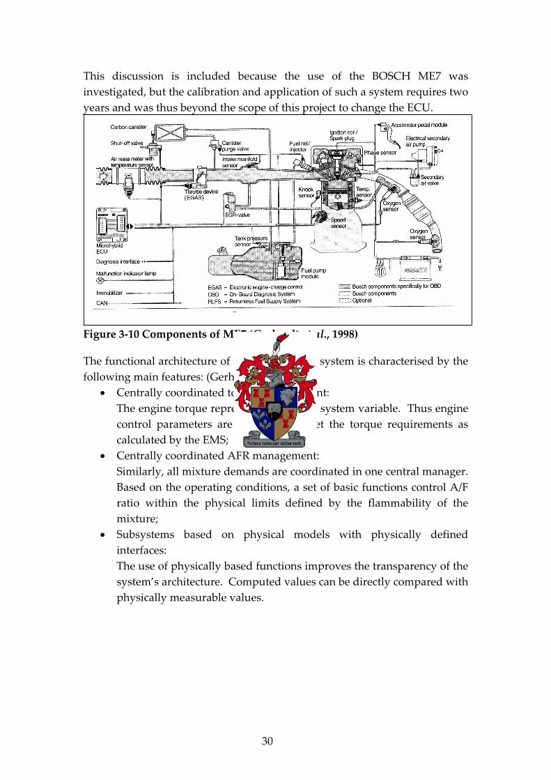
30
This discussion is included because the use of the BOSCH ME7 was
investigated, but the calibration and application of such a system requires two
years and was thus beyond the scope of this project to change the ECU.
Figure 3 10 Components of ME7 (Gerhardt et al., 1998)
The functional architecture of the BOSCH ME7 system is characterised by the
following main features: (Gerhardt et al., 1998):Centrally coordinated torque management:
The engine torque represents the central system variable. Thus engine
control parameters are adjusted to meet the torque requirements as
calculated by the EMS;
Centrally coordinated AFR management:
Similarly, all mixture demands are coordinated in one central manager.
Based on the operating conditions, a set of basic functions control A/F
ratio within the physical limits defined by the flammability of the
mixture;
Subsystems based on physical models with physically defined
interfaces:
The use of physically based functions improves the transparency of the
system’s architecture. Computed values can be directly compared with
physically measurable values.

31
Using physically based functions in combination with centrally coordinated
torque and AFR management allows for an improved handling of function
variants. Due to their relationship to the physical structure, single functions
as well as functionally linked groups of functions, subsystems could easily be
compared with customer’s requests using physically measured values.
Therefore a set of basic platform functions was realised and applied over the
entire EMS family (Gerhardt et al., 1998).
3.3.3. Boost Control
In a spark ignition engine the primary parameter controlling power output is
the amount of air induced into the engine per cycle. By definition
conventional spark ignition engines operate at a stoichiometric or near
stoichiometric air fuel ratio. Thus the amount of fuel injected is directly
proportional to the amount of air induced. The amount of air induced is
dependent on the density of air in the intake manifold. At wide open throttle
(WOT) for a turbocharged engine the density of air in the intake manifold is
proportional to the boost pressure. Thus to control the power output of the
engine, the boost pressure must be controlled.
The boost pressure developed by the compressor is proportional to the
amount of energy extracted by the turbine from the exhaust gas. By using a
by pass valve to route some of the exhaust gas directly to the exhaust system
and not through the turbine, it is possible to control the boost pressure. The
traditional way of controlling the by pass valve (or wastegate) is by actuating
it with a pneumatic piston. The piston is spring loaded, with a predetermined
preload. The preload on the spring determines the opening boost pressure
and the spring stiffness determines the relationship between wastegate
opening area and boost pressure. A typical layout is shown below in Figure
3 11.

32
Figure 3 11 Conventional Boost Control Layout (Audi AG, 1998)
With the increased power and capability of the modern ECU, electronic boost
control is becoming more common. This can be implemented by
manipulating the pressure that acts on the diaphragm of the wastegate
actuator. Manipulation of the pressure can be realised with the use of a 3 way
solenoid valve. A typical layout can be seen in Figure 3 12 and connections
within the valve can be seen in Figure 3 13.
Figure 3 12 Typical Electronic Boost Control Layout (Audi AG, 1998)

33
In the valve’s normal (de energised or OFF) position the wastegate (2) is
connected directly to the boost pressure (3). If the valve is energised
(switched ON) the wastegate (2) is connected to atmosphere (1) and the
wastegate will not open, thus maximum boost will be developed. Switching
the solenoid valve on and off repeatedly, the pressure on the actuator piston
can be varied between atmospheric pressure and the boost pressure. The
actual pressure generated at (2) will depend on the switching duty cycle.
The result is that the higher the switching duty cycle, the lower the pressure
on the actuator piston. This will result in a smaller opening of the wastegate
and thus a higher boost pressure could be developed. The advantage of using
the valve in its normal open position is that, should the electronics fail, the
wastegate will open as in the conventional case, producing a lower boost
pressure than with electronic control.
Figure 3 13 3 way Solenoid Valve (Normally open)
3.4. Engine Performance Simulation
WAVE is a computer aided engineering code developed by Ricardo to
analyse the dynamics of pressure waves, mass flows and energy losses in
ducts, plenums and the intake and exhaust manifolds of various systems and
machines. WAVE provides a fully integrated treatment of time dependent
fluid dynamics and thermodynamics by means of a one dimensional finite
difference formulation incorporating a general thermodynamic treatment of
working fluids including air, air hydrocarbon mixtures, products of
combustion, freons and liquid fuels. In addition, WAVE provides a
completely coupled interface to Ricardo s CFD code, VECTIS, which allows
various system components to be simulated as a full three dimensional
model. Finally, WAVE provides a completely coupled interface to external
models which are user defined to specifically describe the physics in a system
component.

34
WAVE can model general networks of pipes, volumes and junctions in terms
of a set of building blocks, which include:
Constant area or conical pipes or ducts;
Passages with abrupt changes of area;
Junctions of multiple ducts;
Elbows, orifices and plenums;
Terminators such as infinite plenums (ambients) and anechoic
boundaries.
WAVE also includes a library of machinery components such as engine
cylinders, piston compressors, turbocharger compressors and turbines, and
pumps. These components can be attached to the pipe networks to serve as
the sources or absorbers of pulsating flows.
The basic methodology incorporated in WAVE has been extensively tested
against a set of reference test cases (Ricardo, 2002). These included: shock
wave propagation in a duct, pressure wave reflection from closed and open
ends of a duct, steady state flow through a duct with an abrupt change of
cross sectional area, flow through an orifice, pipe flow with friction, pipe flow
with heat transfer and flow through junctions of three ducts.
3.4.1. Flow Modelling
The details of the flow in ducting systems are obtained as a solution of quasi
one dimensional compressible flow equations governing the conservation of
mass, momentum and energy. The duct system is discretized into a series of
small volumes and the governing equations are then written in a finite
difference form for each of these elementary volumes. A staggered mesh
system is used, with equations of mass and energy solved for each volume
and the momentum equation solved for each boundary between volumes.
The equations are written in an explicitly conservative form as:
mdt
dmmass Eq 3 10
sourceshmdt
dmeenergy Eq 3 11
lossesumdxdx
dpA
dt
dmumomentum Eq 3 12

35
The thermodynamic properties of the fluids are based on the appropriate
governing relations, such as perfect gas equations for the thermo chemistry of
hydrocarbon/air mixtures for general C/H/O/N type fuels, or real gas
equations for fluids such as freons or oils.
The solution of the governing equations is obtained by the application of a
finite difference technique utilizing the finite volume approach to the
discretization of the partial differential equations. The time differencing is
based on the explicit technique, with the time step governed by the Courant
condition.
This approach is superior to the method of characteristics, because it does not
require the inaccurate and cumbersome ad hoc treatment of many of the
terms of the governing equations and of the geometry. These ad hoc
treatments, which are inherent in the method of characteristics, introduce
inaccuracies specifically in the areas of source terms such as heat transfer,
friction, and distributed losses, boundary conditions at locations of abrupt
area change, junctions of multiple ducts, and bends. WAVE, on the other
hand, because of its basic formulation and solution technique, is able to
handle these effects accurately and with no special difficulty.
3.4.2. Combustion Modelling
WAVE contains a number of relatively simple but fully integrated combustion
models such as:
Standard diesel combustion;
SI combustion model (Wiebe based);
Stratified charge combustion model.
Since this thesis is focused on SI engines, only the SI combustion model will
be discussed in more detail.
The correlative combustion model for premixed charge spark ignited engines
is based on a Wiebe function relationship widely used to describe the rate of
mass burned in thermodynamic calculations. This relationship allows the
independent input of function shape parameters and of burn duration. It is
known to represent quite well the experimentally observed trends of
combustion heat release. When using the Wiebe correlation, the cumulative
mass fraction burned as a function of crank angle is given by the following:

36
1
1
WEXP
BDURAWIEXPW Eq 3 13
where:W = cumulative mass fraction burned
= crank degrees past start of combustion
BDUR = user entered 10 % – 90 % burn duration in crank degrees
WEXP = user entered Wiebe exponent
AWI = internally calculated parameter to allow BDUR to cover the
range of 10 % 90 %.
When using the Wiebe model, the combustion rate is controlled by three user
defined parameters. These are the location, in degrees, of the 50 % burned
point of the total heat release; the burn duration, in degrees, from 10 % to
90 % mass burned; and the Wiebe function exponent. The main effect of the
Wiebe exponent is the shift of the 10 % and 90 % points with respect to the
50 % point. This is illustrated in Figure 3 14 and Figure 3 15. In both figures
the 50 % burn point and combustion duration were held constant at 10 ˚CA
and 25 ˚CA respectively. It can be seen that a WEXP = 2 shift the 50 % burn
point earlier in respect to the burn duration than would a higher value for
WEXP.
0
0.005
0.01
0.015
0.02
0.025
0.03
0.035
0.04
0.045
30 20 10 0 10 20 30 40 50
Crank Angle Degrees
NormalisedRate/CA
WEXP = 2 WEXP = 4 WEXP = 8
Figure 3 14 Wiebe Combustion Curve Shape

37
0
0.1
0.2
0.3
0.4
0.5
0.6
0.7
0.8
0.9
1
30 20 10 0 10 20 30 40 50
Crank Angle Degrees
WEXP = 2 WEXP = 4 WEXP = 8
Figure 3 15 Wiebe Cumulative Combustion Curve Shape
3.4.3. Modelling of Compressors and Turbines
In WAVE a turbocharger is modelled as two separate components, a
compressor and a turbine. There may be more than one of each in a given
simulation. A compressor may be driven by an associated turbine or may be
gear driven by the engine. Similarly, a turbine may be driven at a fixed speed
for simulation of turbocompounded components. A compressor’s boost
pressure or speed can be controlled by actuating a wastegate or variable
geometry nozzle of its associated turbine. A turbine may be of fixed or
variable geometry with an optional wastegate. Each component is
represented by a map that relates mass flow, pressure ratio, rotational speed
and efficiency. Standard dimensional maps are pre processed for use in
WAVE by the TCMAP pre processor, which smoothes and extends the maps
and produces an input file for WAVE. This is done to allow optional user
prescribed scaling of the turbocharger to match it to an engine.
The compressor and turbine are each modelled as type 1 junctions, which are
plane boundaries between adjacent duct sub volumes. The compressor
junction requires two ducts, one inlet and one or more outlets. Both the fixed
and the variable geometry turbine junctions allow multiple inlet ducts and
one output duct.

38
A variable geometry turbine is defined in WAVE by supplying a series of
turbine performance maps, each at a different nozzle angle (rack position).
The code determines the actual turbine characteristics by interpolating
between the supplied maps to any rack position. An integral wastegate may
be defined for any turbine in the system. WAVE simulates the wastegate
opening as an additional flow path from the entrance duct to the exit duct of
the turbine. A fixed opening integral wastegate can be defined for each
turbine in the system. To model an external wastegate, one which does not
lead directly from the turbine inlet duct to the turbine outlet duct, a separate
flow path around the turbine may be constructed, using an orifice junction or
dashpot driven check valve junction to represent the wastegate itself.
The calculation of flow through a compressor or a turbine is carried out in
WAVE in the following manner. At each time step of the simulation of a
compressor/turbine, the code accesses the appropriate steady state map in a
quasi steady manner. The inputs used to read the maps are the instantaneous
values of inlet pressure and temperature and outlet pressure (values are total
or static as appropriate), and the compressor/turbine speed. The outputs
obtained from the maps are the instantaneous mass flow and adiabatic
efficiency. From these values the simulation computes the resulting
instantaneous mass and enthalpy fluxes out of the compressor or turbine.
Also, the instantaneous work done or extracted by a compressor/turbine is
calculated. The works of the compressor and turbine are integrated in time to
calculate the change of speed of the turbocharger.
For multiple entry turbines, WAVE makes a default assumption that all of the
entries are identical. If a multiple entry turbine is not symmetrical, the user
can override this assumption by assigning individual flow capacities to each
turbine entry. The total mass flow through the turbine is then the sum of the
mass flows calculated separately for each entry. Any leakage between the
multiple entries of the turbine must be accounted for by the user by
constructing a leakage orifice between the entries. For compressors with
multiple exits, the assumption is made that all of the exits are identical. The
above procedures represent a simplified treatment of two unsteady features:
The gas pressure and temperature entering a turbine can be
substantially non uniform in time, while the turbine maps were
acquired under steady state conditions. This introduces an error of
unknown magnitude into the simulation;
Under the conditions of partial admission (twin entry turbines), the
instantaneous mass flow through each entry of the turbine may not be
equal to one half of the full map value as assumed above.

39
Under steady state conditions, the above procedure perfectly reproduces the
steady state map data. The situation under unsteady conditions is less clear.
Comparisons of simulation results to available turbocharged engine data
made by Ricardo suggest that, despite the simplified treatment, the agreement
with data is quite good, at least within the typical inaccuracies due to
measurements of gas temperature and, to a lesser degree, pressures and
speed. (Ricardo, 2002)

40
4. ENGINE SIMULATION
The process of engine design and development can be time consuming and
laborious. If a numerical model can be used to predict engine performance
and calculate mechanical and thermal stresses, the results may be used for
optimisation of the engine. This optimisation may include, but is not limited
to, swept volume, CR, valve timing, turbocharger matching, and inlet and
exhaust manifold geometry. This optimisation may be done with the required
power output and/or reliability as the objective. With the use of numerical
models, the engineer will be able to develop a prototype engine that is much
more refined and closer to the optimum match than would be possible in the
same time without such a tool. Development time, and hence cost is reduced,
resulting in a better end product.
4.1. Engine Simulation Model – 1.6 litre Ford Rocam
Development and modelling of the test engine had previously been done with
WAVE; thus a model representing this engine existed, thus it was not
necessary to build a completely new model. The existing model was updated
to reflect the design changes made to the engine. Changes were made to the
exhaust manifold to accommodate the turbine, the exhaust system was altered
to represent the geometry of the system as used in actual engine testing and
the intake piping was adapted to accommodate the compressor. Figure 4 1
shows the graphical representation of the simulation model.
The values needed for combustion simulation were the Wiebe exponent, burn
duration and 50% burn point. These values were carried over from the
previous model, since no combustion data were initially available to update
these values. Therefore the simulated combustion and actual combustion
might differ.

41
Figure 4 1 Simulation model: Ford RSI Turbo
The design and simulation of the exhaust manifold were done using the old
combustion data from the NA model. Since the comparison between the
exhaust manifold concepts was done with the focus on engine breathing, the
influence of the combustion data was deemed not to be an important factor. It
was only after everything was built and the engine was set up and running
that combustion data were measured and used for final correlation between
the actual test data and simulations.
4.2. Engine Optimisation
When developing an up rated engine or doing a turbocharged conversion on
a NA engine, a target output must be set and decisions must be made on
which engine parameters may be changed in order to achieve the desired
output. As mentioned earlier, there are numerous parameters that can be
changed or optimised. All possible changes can be classified as primary and
secondary changes.

42
Engine design, performance simulation and optimisation are iterative
procedures; thus it is very difficult to separate the discussions of engine
simulation and optimisation from that of the next section, namely design and
modification. Primary and secondary changes will be indicated in this
section, but the influence of and the decisions taken regarding them will be
discussed in the next section.
In this project, where a turbocharger conversion is done on a NA engine, the
primary changes would be all changes that are necessary to fit the
turbocharger to the engine and make the basic configuration work. These
primary changes would typically include:
Redesigned exhaust manifold to accommodate the turbocharger;
Connecting the turbine outlet to the exhaust pipe;
Rerouting the clean air piping to include compressor before the
intake manifold;
Supplying oil to the turbocharger bearings and returning it to
the sump;
Supplying water for the cooling of the turbocharger bearings;
Upgrading the fuel injectors and fuel pressure regulator to
supply the extra fuel needed;
Changing the manifold absolute pressure (MAP) sensor to
enable boost pressure measurement by the ECU;
Adjusting fuelling and timing maps on the ECU.
Secondary changes can be defined as those changes that are not essentially
necessary, but would be beneficial to make. These changes could entail the
following:
Charge air cooling;
Valve timing optimisation;
Lowering of CR;
Electronic boost control;
Electronic throttle control.
Simulations at an early stage indicated that the objectives could be met with
only the primary changes. Therefore none of the secondary changes was
made, but when the simulation model has been correlated to the actual
engine, they could be used to illustrate the advantage that each secondary
change could have.

43
4.2.1. Modelling Strategy for Wastegate Control
The simulation package used has the capability to control the wastegate
opening area to a set target or limit on Brake Mean Effective Pressure (BMEP),
boost pressure or compressor speed. In reality, if a pneumatic actuator is
used, the boost pressure developed is proportional to the stiffness of the
spring and the opening pressure is proportional to the preset compression of
the spring. This relationship can be seen in Figure 4 2. The data were
obtained by doing a simple test with the actual wastegate actuator fitted to the
turbocharger used.
0
100
200
300
400
500
10 20 30 40 50 60 70 80
Boost Pressure [kPa]
WastegateArea[mm2]
0
3
6
9
12
15
RackTravel[mm]
Wastegate Area Travel
Figure 4 2 Measured Rack Travel and Calculated Wastegate Area versus
Boost Pressure
Pressure was applied with a hand pump and then the rack travel was
measured. Because the area cannot be measured directly, it has to be
calculated. With reference to Figure 4 3, the physical opening area can be
calculated by assuming that the flow area is the surface area of a cylinder that
is cut by a plane that is at an angle to the centreline of the cylinder. The flow
height BB’, height of the centreline of the cut cylinder, is equal to the travel
height AA’ multiplied by the ratio OB:OA. Thus the area can be calculated by
Eq 4 1.
OA
OBAARArea 2 Eq 4 1

44
If the flow area calculated with Eq 4 1 is bigger than the area of the hole in the
casing of the turbine, the area of the hole is used. This explains why the
wastegate area in Figure 4 2 remains constant for boost pressures exceeding
55 kPa. Thus the maximum wastegate area is equal to the area of the hole in
the turbine casing, which is equal to 490 mm2 for the turbocharger being used.
Flow Height
O
Rack travel
Flow Height
A
OB
A
A’
OO B
B’
Figure 4 3 Wastegate Area Calculation
A Visual Basic program (WG_control) was written to control the wastegate
area in an iterative manner until the area versus boost pressure corresponds
to the spring stiffness and preset compression. A simplified algorithm for
WG_control is outlined below:
Execute WAVE simulation with user specified starting value for
wastegate area;
Read results from output file after simulation finished;
Determine shortest distance between operating point and wastegate
characteristic line;
Adjust wastegate area in input file and execute WAVE simulation;
Repeat process until operating point lies within the specified tolerance
from wastegate characteristic line.
This code was written as a subroutine that it could easily be incorporated into
another program to fulfil this function.

45
4.2.2. Exhaust Manifold Simulation
The exhaust manifold had to be redesigned in order to accommodate the
turbocharger’s turbine. Two concepts for the exhaust manifold were
evaluated with the aid of simulations. The objective was to compare the
amount of internal exhaust gas recirculation (EGR) and exhaust manifold
pressure of the two concepts.
The detailed concepts are discussed in section 5, but the modelling of the
concepts in WAVE will be discussed here. Figure 5 3 and Figure 5 5 show the
computer aided design (CAD) models of the two concepts.
The two concepts are built up of ducts, orifices and complex junctions in
WAVE. The representation is shown in Figure 4 4 and Figure 4 5
respectively. Concept 1 consists of 2 complex junctions, 12 ducts and 6
orifices. Orifices are used to connect two ducts together. If the ducts are of
the same diameter, the orifice plays no role other than connecting two ducts,
but if the diameters differ, it acts as an abrupt change in area. Complex
junctions were used to model the junctions between the different cylinders in
order to model the flow and duct orientation correctly. Complex junctions
take into account the duct orientation and represent the volume where two or
more ducts join together.
Figure 4 4 Simulation Model of Exhaust Manifold: Concept 1
Concept 2 consists of 15 ducts, 8 orifices and 3 complex junctions. Concept 2
has more components to account for the simple pulse converters used. Ducts
6013, 6016, 6018, 6022, 6023 and 6091 cross sectional area decreases in the flow
direction to simulate nozzles. The complex junctions are used to simulate the
collector between two nozzles and connection to the next duct.

46
Figure 4 5 Simulation Model of Exhaust Manifold: Concept 2
Simulations were done with all inputs identical but with the two different
exhaust manifold concepts. During the simulations the focus was shifted to
the turbocharger’s performance and the engine’s breathing characteristics.
The approach taken was to run engine simulations in such a way as to
emulate the methodology that would have been used in an engine prototype
development process. Thus the wastegate was opened according to a spring
stiffness that was pre defined. Since the actual turbocharger used for this
project came with a wastegate actuator, its standard opening characteristics
were used in the simulation. This test was done at different engine speeds in
order to investigate each concept’s performance across the engine’s entire
operating speed range.
4.2.3. Valve Timing Optimisation
The valve timing plays an important role on the breathing of an engine. The
requirements for a turbocharged engine differ from that of a naturally
aspirated engine. In general the valve timing of a naturally aspirated engine
can be optimised for either higher torque at low engine speeds, compromising
power at high engine speeds or vice versa.
In general for NA engines the exhaust valve closure (EVC) and intake valve
opening (IVO) are the important parameters, whereas on turbocharged
engines the exhaust valve opening (EVO) and intake valve closure (IVC) are
more important (Watson & Janota, 1984). Furthermore, the amount of valve
overlap plays a significant role. Valve overlap is defined as the crank angle
during which both exhaust and intake valves of the same cylinder are open.

47
Another factor that plays a significant role is the amount of exhaust valve
overlap. This can be defined as the crank angle that the exhaust valves of two
cylinders, which fire in succession and are on the same exhaust manifold, are
open simultaneously.
As mentioned earlier, valve timing optimisation falls under the secondary
engine changes. This optimisation was done only using simulations and is
used to illustrate its advantages.
4.2.3.1. Optimisation Strategy
Optimising the valve timing and lift is a trade off between higher torque at
low engine speeds and power at high engine speeds. The initial aim of this
project was to achieve a torque curve, as flat as possible, over a wide engine
operating speed range at 150 N m and to produce 100 kW at 6366 rev/min.
This odd engine speed was due to the fact that the gearbox that this engine is
mostly used with, was rated at 150 N m maximum; therefore to achieve
100 kW at this torque the engine speed must be 6366 rev/min.
Thus optimising the valve timing for low engine speeds would result in very
little boost being required to achieve the target of 150 N m, but with high
boost being required at high engine speeds. Due to the fact that the
compression process in the compressor is not isentropic and the higher the
boost pressure, the higher the compressed air temperature, the initial charge
temperature would be higher, which would make the engine even more
susceptible to knock because initial charge temperature and pressure would
be higher than normal.
If the valve timing was optimised for a specific engine speed, the same airflow
could be achieved with lower boost pressure than when the valve timing was
not optimised, but with higher boost. Therefore when considering the above,
it was decided to optimise the valve timing for high engine speeds in order to
decrease the boost pressure necessary to achieve the 100 kW target, while
higher boost pressure would be used at low engine speeds to achieve the
150 N m target.
However, the higher boost pressure at low engine speeds could result in a
situation where the boost pressure is high enough and the airflow is low
enough to cause the compressor to surge. Thus care must be taken to ensure
that the compressor operates with an adequate safety margin from the surge
line on the compressor map.

48
Knock at low engine speeds are generally more severe and damaging than at
high engine speeds. The boost pressure and charge air temperature would be
higher than optimal at low engine speeds, but would still be lower than at
high engine speeds, even if the valve timing is optimised for high engine
speeds. Therefore it was not expected that knock would occur at low engine
speeds. Since knock was not simulated and the optimised valve timing
would not be implemented, it was assumed that knock would not occur for
the purpose of this investigation.
4.2.3.2. Full Factorial Simulation
The optimisation of valve timing and lift is basically the optimisation of a
function which is not explicitly known and which has six variables (EVO,
EVC, IVO, IVC, exhaust valve lift, intake valve lift). There exist numerous
optimisation algorithms each applicable to certain kinds of problems (Press etal., 2001). Most optimisation algorithms require quite a number of iterations
before arriving at a solution. Therefore it was decided that, as a starting
point, a full factorial optimisation would be done.
Valve lift is limited by the maximum acceleration the valve train can
withstand. The acceleration is inversely proportional to the time the valve is
open and proportional to the valve lift. The result would be that the longer a
valve is open, the more lift is possible and vice versa for a given maximum
acceleration. Thus to keep the maximum acceleration the same, the amount of
lift must be adjusted according to the valve open time. In the full factorial
search the simplification was made that the lift for both the valves remains
constant. With this decision the variables were reduced to four.
Assigning four values to each variable it resulted in four to the power of four
simulations, which is equal to 256. Table 4 1 lists the initial values used for
each variable. This would give a relatively coarse search, but refinement can
be done in an iterative way. The simulations only require computer time and
not actual testing and set up time, thus it was cost effective to perform such a
full factorial search. The search was done at an engine speed of 6366 rev/min
and 2000 rev/min. 256 simulations at a single engine speed took about five
days to complete on a personal computer with an AMD 1.2 GHz Duron
processor and with 128 MB of memory.

49
Table 4 1 Initial Values for Full Factorial Valve Optimisation
IVO IVC EVO EVC
270 540 90 360
300 570 130 390
330 600 150 420
360 630 180 450
After the simulations were completed, the results were sorted in order of
descending engine torque and increasing boost pressure. Thus the top results
were the highest torque with the lowest boost pressure. The top 20 results
showed that the best IVC was as late as possible. Thus IVC was held constant
during further refinement. A second optimisation process was undertaken
with only 3 variables and 5 values for each. After the refined optimisation
was completed, the results were again sorted as described above. The search
was iterated until each of the remaining 3 variables’ values was within 1
degree of each other.
The end results for each speed opposed to the standard engine’s valve timing
can be summarised as in Table 4 2. It can be seen that the required valve
timing differs a lot from low to high engine speeds. The standard engine’s
intake valve timing fits between the optimised results, but that found for the
exhaust valve is totally different. This was due to the different breathing
characteristics caused by the turbocharger. The valve overlap at 6366 rev/min
of 63°CA was close to that on the standard engine of 70°CA.
Table 4 2 Full Factorial Results
Engine Speed
[rev/min]
IVO
[°CA ATDC]
IVC
[°CA ATDC]
EVO
[°CA ATDC]
EVC
[°CA ATDC]
2000 301 580 172 421
6366 342 630 125 405
STD Engine 328 614 112 398

50
4.2.3.3. Optimisation Using a Search Algorithm
In the previous section valve optimisation was done at two engine speeds.
Thus a solution for both the high and low engine speeds was obtained. This
would not necessarily result in a flat torque curve. The ability to optimise the
wastegate actuator together with the valve timing to obtain the desired torque
curve could not be done using the full factorial method. Since the target was
a nearly flat torque curve over a wide as possible engine speed range, an
optimisation problem was setup to optimise for the whole engine speed
range. The target torque curve can be specified and the optimisation
algorithm will optimise the valve timing and wastegate actuators
characteristics to obtain the desired torque curve while using minimal boost
pressure.
Increasing the number of variables increases the complexity of the
optimisation process considerably. In order to make a decision on which
optimising algorithm must be used, some of the characteristics of the function
that must be optimised must be known. The function in this specific case had
multiple variables, was not explicitly known and thus it was impossible to
calculate the function’s gradient (derivative) directly. The method of finite
differences could have been used to determine the function’s gradient but this
would have resulted in more function evaluations (simulations), which is time
consuming. The fact that the output torque doesn’t vary much with small
variations in valve timing (0.25 degrees) further complicates the
determination of the function’s gradient.
It was decided to use a direct search method, such as the Simplex method.
There are various variations of the Simplex method available. The Nelder
Mead Simplex algorithm was the choice from Press W H, et al.(2001). The
program example was easily rewritten in Visual Basic and was combined with
the wastegate control program mentioned earlier enabling optimisation of the
valve timing as well as the wastegate actuator characteristics.
Including the wastegate spring stiffness (GRAD) and preload (PRESET) into
the optimisation the variables were increased to six, namely: IVO, IVC, EVO,
EVC, GRAD and PRESET. The same simplification on valve lift was made as
in the full factorial search, it was kept constant.

51
Considering these facts, the following strategy for valve optimisation was
developed:
1. Set initial values of IVO, IVC, EVO, EVC, GRAD, PRESET;
2. Determine initial wastegate area;
3. Run wave simulation;
4. Calculate new wastegate area based on boost pressure developed;
5. Adjust wastegate area to actuator characteristics;
6. Repeat steps 3 to 5 until all operating points correspond to actuator
characteristics;
7. Evaluate torque curve;
8. Calculate new values for variables;
9. Repeat steps 3 to 5 until all operating points are on desired line;
10. Repeat steps 7 to 9 until no further improvement is found.
When the torque curve is evaluated it is actually compared to the target
torque curve that the user specified. The optimisation program was
programmed in such a way that a specific torque can be specified at each
speed and also a weighing factor indicating its importance. The error that the
optimisation program minimises can be expressed in Eq 4 2. Including the
boost pressure in the error will have the result that the optimisation seeks the
minimum boost pressure.
1
.n
i i i i
i
Error Tt Tp C Pboost Eq 4 2
Where: Tti = target torqueTpi = predicted torque
Ci = weighing factor
Pboosti = boost pressuren = number of speeds evaluated in simulation.
The initial values as well as the optimised results after 30 iterations on a
model with exhaust manifold concept #1 are shown in Table 4 3; it took about
three weeks to complete 30 iterations. The torque curves for the standard and
optimised results can be compared in Figure 4 6 with the ideal torque curve.

52
Table 4 3 Simplex Optimisation Results (30 iterations)
Variable Initial Optimised
IVO 328 329
IVC 614 621.8
EVO 112 112.4
EVC 398 390.7
GRAD 20 19.1
PRESET 25 26.7
ERROR 63.4 24.7
Further investigation into the torque limit on the gearbox proved that
150 N m was not the limit. Therefore the restriction of a torque limitation was
removed. Since 6366 rev/min was above the standard engine’s rev limiter
(6250 rev/min), it was decided to lower the engine speed at which peak power
would be developed. The target torque curve was constructed by calculating
the required torque to deliver 100 kW from 5000 rev/min up to 5500 rev/min.
This resulted in 191 N m and 174 N m respectively. Thus 191 N m was then
assumed from 2500 rev/min to 5000 rev/min and 174 N m for both
2000 rev/min and 5500 rev/min and each point were given the same weighing
factor.
150
155
160
165
170
175
180
185
190
195
1500 2000 2500 3000 3500 4000 4500 5000 5500 6000
Engine Speed [rev/min]
Torque[Nm]
Ideal Initial Optimised
Figure 4 6 Effect of Optimised Valve and Wastegate Settings on Torque

53
It can be seen that with only 30 iterations the improvement was considerable.
This improvement would not have been possible if only the valve timing was
altered without adjusting the wastegate settings. This optimisation tool
enables the user to specify any torque curve and the simulation will iterate
until the best possible solution using minimal boost pressure is found given
the constraints.
To simplify the optimisation and to speed it up, one or more of the variables
can be made constant. Since the magnitude of the different variables in the
optimisation varies between 20 and 600, scaling these parameters to the same
magnitude also benefited the optimisation. See APPENDIX A for the Nelder
Mead simplex method algorithm that was implemented in the optimisation
program as well as the scaling procedure.
4.3. Exhaust Manifold Concept Evaluation
As mentioned previously (section 4.2.2) the focus of the exhaust concept
evaluation is the breathing characteristics of the engine, pressure difference
across the engine and turbine and compressor performance. These were all
compared using the same wastegate actuator settings to control the boost
pressure.
Two exhaust manifold concepts were designed, one with easy manufacturing
and assembly as the highest priority and is referred to as concept 1. The
second concept was designed for optimal utilisation of the pulse energy in the
exhaust gas and making use of simple pulse converters to limit the amount of
pulse interference. This design is referred to as concept 2.
In Figure 4 7 it can be seen that the relationship between wastegate area and
boost pressure for both concepts fell exactly on the same line, thus the actual
actuator appears to have been simulated correctly in both cases. It is
important to note that the individual points are not exactly coincident. It can
be seen that concept 1 (C1) developed a higher boost pressure and thus the
wastegate area is proportionally bigger. But when considering the torque
developed as shown in Figure 4 8, concept 2 (C2) developed about 1 N m
more torque, which is a relatively small difference.

54
0
0.2
0.4
0.6
0.8
1
1.2
1.4
1.6
1.26 1.27 1.28 1.29 1.3 1.31 1.32 1.33
Boost Pressure [bar]
WastegateArea[cm
2]
C1 C2
Figure 4 7 Exhaust Concept Evaluation: Wastegate Area
As can be seen from Figure 4 8 the difference in torque developed varies
between 0.6 N m and nearly 1 N m and that C2 develops more torque than
C1. If the boost pressure developed by C2 was lower, while the torque
developed by C2 was greater, C2 must have a higher volumetric efficiency.
This is illustrated in Figure 4 9, which compares the volumetric efficiency.
130
140
150
160
170
180
1000 2000 3000 4000 5000 6000 7000
Engine Speed [rev/min]
Torque[Nm]
1
0.8
0.6
0.4
0.2
0
Difference(C1C2)
C1 C2 delta
Figure 4 8 Exhaust Concept Evaluation: Torque
The difference in volumetric efficiency is small less than 0.53%. The slightly
higher volumetric efficiency can directly be translated into a higher airflow
(Figure 4 10) through the engine.

55
98
100
102
104
106
108
110
112
1000 2000 3000 4000 5000 6000 7000
Engine Speed [rev/min]
VolumetricEfficiency[%
0.6
0.5
0.4
0.3
0.2
0.1
0
Difference(C1C2
C1 C2 delta
Figure 4 9 Exhaust Concept Evaluation: Volumetric Efficiency
At 6000 rev/min the difference in airflow is 1.24 kg/hr, which is a small
difference but is significant enough to make a 1 N m difference.
100
150
200
250
300
350
1000 2000 3000 4000 5000 6000 7000
Engine Speed [rev/min]
Airflow[kg/h]
1.4
1.2
1
0.8
0.6
0.4
0.2
0
Difference(C1C2)
C1 C2 delta
Figure 4 10 Exhaust Concept Evaluation: Airflow

56
When comparing the compressor and turbine efficiency, they were all within
0.5% of each other; thus it is too small to be significant. When comparing the
average residual mass (Figure 4 11) in all 4 cylinders, it is clear why C2
develops more torque than C1. C2 has less residual mass inside its cylinders;
thus it has more space for a fresh mixture of air and fuel and can therefore
develop more torque. This is also the reason why the volumetric efficiency
was higher for C2.
It is evident from Figure 4 7 that C1 develops a higher boost pressure than C2
and when comparing the average turbine inlet pressures the difference is less
than 0.2 %, thus extremely small. Thus it is assumed that the higher residual
mass of C1 could be attributed to the effect of pulse interference, causing
reverse flow over the exhaust valve before closure or reverse flow over the
inlet valve during valve overlap. In order to prove this assumption the mass
flow over the valves should have been examined.
5
5.5
6
6.5
7
1000 2000 3000 4000 5000 6000 7000
Engine Speed [rev/min]
Avg.ResidualMass[%]
2
2.5
3
3.5
Difference(C1C2)
C1 C2 delta
Figure 4 11 Exhaust Concept Evaluation: Average Residual Mass
Considering the above results, C2 is the better concept of the two, but it is
only marginally better. Optimisation could be used to optimise the nozzles of
the pulse converters, but optimisation might also be used to optimise C1 for
pipe diameters and junction specifics. The optimisation of C2 or C1 might not
be worth the effort.

57
When considering the advantages and disadvantages of each concept,
simplicity, performance and practicality need to be taken into account. C1
was the obvious choice, since its performance is only slightly less than C2, and
it was very much simpler and easier to manufacture than C2. The location of
the bolts on the turbine inlet would interfere with C2, making assembly
nearly impossible. C1 was thus manufactured for physical engine tests.

58
5. EXPERIMENTAL APPARATUS
Keeping in mind that the engine with a turbocharger and all the modifications
must still fit into the engine bay of the original vehicle without modifications
to the firewall, packaging is a significant challenge.
In this section all designed modifications are discussed in detail. The design
process followed will not be discussed in detail, but only the final concepts
and relevant manufacturing details will be highlighted. The difference
between the standard and turbocharged engine is summarised in Table 2 1.
5.1. Exhaust Manifold Design
Designing an exhaust manifold that would fit in the engine bay, make use of
the exhaust energy in the most efficient way and be easy to manufacture is an
optimisation problem that has to satisfy very challenging criteria. On the
basis of simulation results, which indicated small differences in performance
between different concepts, it was decided that the manifold that was easiest
to manufacture and that would fit was the solution that would be used. It
may not be the most efficient manifold, but it would work satisfactory. Thus
fitting the turbocharger became a packaging challenge.
The spatial constraints are very tight, since no space can be wasted in a
passenger car. The fact that the engine is of the cross flow type with the inlet
manifold on one side and the exhaust manifold on the other side complicates
matter further. The engine is transversely mounted, with the exhaust to the
firewall. The original equipment manufacturer (OEM) specifies that there
must at least be a space of 25 mm between the engine and its attachments, e.g.
exhaust manifold or turbocharger and the firewall. A CAD model of the
complete engine bay was not available to the researcher, thus position
measuring had to be done on the actual car.
A positioning rig (Figure 5 1) was designed and manufactured to enable the
researcher to position the turbocharger, and then measure the position
relative to the engine. These measurements were then entered into CAD and
paths for the exhaust runners constructed from standard available pipe sizes
and bends. If a solution could not be found, the position of the turbocharger
had to be altered. This required that the new position had to be checked in
the actual engine bay, before it could be finalised. Two exhaust manifold
concepts were modelled and evaluated with the aid of simulation as
discussed in the previous section.

59
Figure 5 1 Positioning Rig
The positioning rig was bolted to the engine with the exhaust manifold studs.
It then had three sliders with locknuts to make adjustment in the x, y and z
direction possible. The turbocharger was also bolted to the rig and could be
rotated about the z axis in order to correctly position the turbocharger. The
position of the turbocharger was then easily measured by measuring the
distances along the three axes and the rotation about the z axis. These
measurements could then be entered into CAD.
The strength calculations that were of interest were whether the manifold
would be able to withstand the pressures and be structurally strong enough to
support the turbocharger when operating at high temperatures.
Before analysing the two concepts for the exhaust manifold layout, pulse
interference and how its disadvantages can be limited will be discussed.
Pulse interference can seriously compromise the gas exchange process, by
causing reverse flow into the cylinder just before EVC.

60
5.1.1. Pulse interference
When using a single turbine with a single entry, on an engine with more than
3 cylinders, it is inevitable that pulse interference will occur. Pulse
interference occurs when the exhaust valve of a cylinder is nearing its closing
and the exhaust valve of another cylinder opens. The pressure in the latter
cylinder is much higher than in the manifold. This will cause a pressure wave
travelling at sonic speed to travel towards the exhaust valves of the other
cylinders. If the former cylinder’s exhaust valve is still open, reverse flow can
be induced and the cylinder will be filled with exhaust gases. Interference is
likely to occur between: 1 3, 3 4, 4 2 and 2 1, where the first digit denotes the
cylinder nearing closure and the second denotes the cylinder whose exhaust
valve opens. These combinations are characteristic of a 4 stroke four cylinder
engine with firing order: 1 3 4 2. This can be clearly seen on the valve timing
diagram in Figure 5 2. It is also possible that a pressure wave travels toward
the turbine entry and gets reflected at the nozzle. It then runs back to the
cylinder where it came from. These kinds of reflections are called second
order reflected waves. There are even higher order reflections, but their
significance are usually negligible (Watson & Janota, 1984).
0
1
2
3
4
0 180 360 540 720
Crank Angle Degrees
Cylinder
Inlet Valve Exhaust Valve
Figure 5 2 Four cylinder engine s valve timing (firing order 1 3 4 2)
The question may arise: how is pulse interference overcome? The most
obvious way is by making sure that the exhaust valve overlap period is
shorter than the time needed for a pressure wave to travel from one exhaust
port to the next. This means that a very short valve open time must be used
or very long exhaust runners must be used. Both cases could cause serious
restriction to the breathing ability of the engine.

61
Another way of overcoming pulse interference is by grouping the cylinders
together in such a manner that there is no exhaust valve overlap on the
grouped cylinders. From Figure 5 2 it can be seen that there is no exhaust
overlap between cylinders 1 4 and 2 3. Thus the best way would be by
grouping these cylinders together. Joining the two groups of 1 4 and 2 3
together might again result in interference, but if a twin entry turbine is used
pulse interference can be substantially reduced or even eliminated. The
disadvantages of twin entry turbines are that they are more expensive and,
due to the lower frequency at which the pulses arrive at the entries, they
usually operate at a slightly lower efficiency than a single entry turbine.
5.1.2. Exhaust Manifold: Concept 1
Concept 1 shown in Figure 5 3 is the manifold that is the easiest to
manufacture, simple to model, easy to assemble and it fits in the confined
space. The manifold volume is small, but with short bends and sharp corners,
it is not the ideal pulse system. Owing to the small volume, one will be able
to harness some of the pulse energy. The disadvantage of such a manifold is
that pulse interference is unavoidable. The flow path from cylinder #4 to the
turbine entry makes a very sharp turn and a collector is absent at the
transition from the three into one junction.
Figure 5 3 Exhaust manifold: Concept 1, CAD model

62
The pipes used to make up concept 1 are mild steel, have an inside diameter
of 34.9 mm and a wall thickness of 1.6 mm. This was a standard pipe size for
exhausts. The shortest centreline radius available on bends was 75 mm. The
flange that fitted against the engine was laser cut from mild steel and is
10 mm thick. The flange that fitted against the turbine was also made from
10 mm mild steel, but was hand cut. Both flanges were skimmed after
welding to ensure flatness.
The strength calculations were based on an internal peak pressure of 2.5 bar
absolute, the turbocharger weighs 5 kg and the exhaust manifold temperature
was assumed to be 700 °C. A safety factor of 4 was implemented due to the
fact that the exact temperatures and instantaneous pressures were not known.
Material properties of mild steel at high temperatures can be found in Table
5 1.
Table 5 1 Material Properties of Mild Steel at High Temperatures (British
Iron and Steel Research Association Metallurgy, 1953)
Temperature [°C] Yield Strength [MPa] Young’s Modulus [GPa]
600 80 36
700 37 16.5
800 18 8
900 7 3
The manifold could be simplified by considering a thin walled pressure vessel
with internal pressure Pi, which is clamped in on the one side and a force on
the other similar to the classic cantilever example (Figure 5 4).
The stresses for each case (pressure vessel and cantilever) were calculated
using Eq 5 1 and Eq 5 2 and then added to give the total stress in the Zdirection.

63
Figure 5 4 Exhaust Manifold Force Diagram
The yield strength in Table 5 1 was then divided by the total stress calculated
to give the safety factor.
t
trP oiPz
2
).(,
Eq 5 1
I
rLF oFz
..,
Eq 5 2
Where: Pi is the internal pressure (2.5 bar)ro is the outside radius (19.05 mm)
t is the wall thickness (1.6 mm)
F is weight of the turbocharger (5 kg 50 N)
L is the distance from the clamped edge of manifold to the
centre of mass of the turbocharger (103 mm)
I is the second moment of area of the cylinder about an axis
through the centre.
The safety factor was found to be 9; this was larger than what was considered
to acceptable for a temperature of 700°C. Thus higher temperatures were also
considered. For a temperature of 800°C the safety factor was calculated to be
4 and for a temperature of 900°C the safety factor was found to be 2. Due to
the engine durability criteria, exhaust temperatures above 900°C are avoided
during the calibration of the engine. Thus assuming a 200°C difference
between the gas and the wall temperature it can be concluded that this
manifold will be strong enough.

64
5.1.3. Exhaust Manifold: Concept 2
Concept 2 (Figure 5 5) may initially appear simpler, but is actually much
more complex. Simple pulse converters are used at each 2 1 junction, thus
totalling 3 pulse converters. The advantage of such a manifold is that short
runners are used; thus the manifold volume is smaller than that of concept 1
and consequently more of the pulse energy could be harnessed. The
disadvantages of concept 2 are that it is more complex, thus more difficult to
manufacture, and assembly would be complicated due to the placement of the
bolts at the turbine entry.
Figure 5 5 Exhaust Manifold: Concept 2, CAD model
The simple pulse converters were based on a nozzle area ratio of 0.65 and the
throat area ratio 0.68. This combination was chosen so that the minimum
nozzle area specified by Watson and Janota (1984) was used and the throat
area was the same as the turbine entry. Strength calculations where not done
on this concept, because it would not be manufactured. It was, however, also
modelled in WAVE to compare its performance with concept 1 and the results
are presented in 4.2.2.
5.2. Intake Piping Design
The intake piping includes all the pipes from the air cleaner to the compressor
and from the compressor to the intake manifold. The major challenge was
packaging and the strength of these pipes was never a concern, thus no
strength calculations will be shown.

65
5.2.1. Pre Compressor Pipe
It was decided that the standard air cleaner would be used, since it gets fresh
air from the front of the engine bay, thus it would be the coolest air.
Packaging was mainly done on the actual car by building a prototype with
cardboard and then altering as was necessary. Due to the complexity and
packaging of the whole engine and where the pipe fits into the engine bay, it
cannot be shown on a photograph, but the CAD model can be seen in Figure
5 6. The pipe sizes were pre determined, since the pipe that comes from the
air cleaner is fixed and the compressor intake diameter is fixed, thus a
connection pipe that would fit into the engine bay and have the above
mentioned diameters needed to be designed.
After fitting and measuring different combination and configurations the best
and easiest solution was found. It was made up of a straight section with a
60 mm outside diameter (OD), a short radius 90° bend, and a reducer to
40 mm OD, since that is the inlet diameter of the compressor. The short
radius bend was only available in stainless steel, with an OD of 63 mm and
centreline radius of 100 mm. The straight pipe had to be flared to join
properly to the bend. A suitable standard reducer could not be found, thus it
had to be made from a solid round bar, thus reducing from 63 mm to 40 mm.
All the parts were welded together and painted for protection against
corrosion.
Figure 5 6 Pre Compressor Pipe

66
5.2.2. Post Compressor Pipe
The post compressor pipe extends from the compressor outlet to the intake
manifold, where it joins up with the throttle body. Since the compressor
outlet is very near to the exhaust manifold, rubber hose that could withstand
the pressure would not be able to withstand the temperature. Thus the
second choice of material for the pipe was mild steel. The outlet diameter of
the compressor is 50 mm OD and the throttle body has an OD of 60 mm. To
keep the pressure drop over the post compressor pipe as small as possible, it
was decided to use the biggest diameter (60 mm) for as much as possible of
the pipe.
On the compressor side it was necessary for a very sharp bend to clear and
get as far as possible away from the exhaust manifold. The only option was to
cut two 50 mm pipes at an angle and then weld these two together. This,
however, leaves a very sharp bend with sharp corners. Therefore it was
decided to put 3 guide vanes in the bend to direct the flow. Guidelines on
calculating the pressure drop for such bends were found in Kröger (1998), but
no guidelines for the design were available. Van der Spuy (2004), a specialist
in turbomachinary and compressible flow, was consulted. He suggested the
layout and size of the guide vanes. A cross section of this bend is shown in
Figure 5 7.
Figure 5 7 Guide Vanes in a Sharp Bend

67
The complete pipe is composed of the sharp bend followed directly by a
diffuser from 50 mm to 60 mm OD. The diffuser follows into a 90° bend, then
a straight section and is completed with another 90° bend which fits against
the throttle body. The CAD model of the complete post compressor pipe is
show in Figure 5 8.
Figure 5 8 Post Compressor Pipe
Special high temperature silicon hose with inside diameter (ID) 50 mm and
60 mm respectively was used to connect the compressor outlet to the post
compressor pipe and the post compressor pipe to the throttle body. The
hoses were secured with hose clamps on each side.
The post compressor pipe had to withstand the boost temperatures and
pressures. In this case the boost pressure was never above 1 bar and the boost
temperature never above 100°C. Thus it was clear that a mild steel pipe with
wall thickness of 1.6 mm would never operate anyway near its yield strength.
5.3. Variable Wastegate Actuator Design
Since electronic boost control is a complex matter on its own, the need for an
actuator that can easily be adjusted to accomplish different boost pressures
was identified. The requirements of such a variable wastegate actuator
(VWA) were that both the spring stiffness and pre load on the spring must be
independently adjustable.

68
Different concepts were evaluated and the final concept is shown in Figure
5 9. The spring stiffness can be adjusted by adjusting the number of active
coils and the preload can be adjusted by adjusting the locknuts on the rack as
on a normal turbocharger with a wastegate configuration.
Figure 5 9 Variable Wastegate Actuator
The working and function of the parts are discussed with reference to Figure
5 9. Pressure is supplied to the actuator via the hose tail (1) and acts as the
input to the actuator. Part 2 forms a lid for the pressure chamber. Part 3 is the
diaphragm, which deflects to push the plunger (13) that is connected to the
rack (10), which acts as the output and opens the wastegate. The rack screws
into the plunger and is locked with a locknut (12). The spring (9) was ground
flat on the plunger’s side and the tip was turned radially inward to form a tip
that fits into a slot in the plunger. This stops the spring from turning
independently of the plunger. The combination of parts 7 and 8 locked
together with a grubscrew (11) forms an adjusting mechanism to adjust the
number of active spring coils. Parts 4 and 6 screw into each other to adjust the
distance between the diaphragm and part 8. This adjustment allows
independent setting of the number active coils and the amount of preload on
the spring. Parts 4 and 6 are locked together with a locknut (5). The lid (2),
diaphragm (3) and part 4 were all held together by six cap screws.

69
The VWA was tested with different diaphragms. Since the diaphragm must
deform to push the plunger and wastegate open, it is necessary for it to have a
high level of elasticity, withstand gasoline fumes and be able to withstand
high temperatures. This implies that the opening characteristic of the
wastegate is not only dependent on the spring stiffness, but also on the
characteristics of the diaphragm. The combined characteristics of the spring
and diaphragm caused the relation of rack travel against pressure to be non
linear as can be seen in Figure 5 10. The diaphragm was made of rubber.
This rubber was made from a mixture of natural and synthetic rubber. This
rubber diaphragm was not resistant to gasoline; however, the little that it
would be exposed to would not harm it for the duration of a test. The
wastegate actuator was tested with two different rubber compounds.
Compound 1 was red and 3 mm thick while compound 2 was black and about
1.5 mm thick.. The data presented in Figure 5 10 were measured with a very
stiff spring. Actual testing was done using compound 1.
Commercially available wastegate actuators that are supplied with the
turbocharger do not rely on the diaphragm to deform. In fact, the diaphragm
is non elastic. The diaphragm is preformed and looks like a woven material
coated with some kind of rubber to make it airtight. The actuator’s
construction is such that the diaphragm moves without elastic deformation.
0
2
4
6
8
10
12
14
16
18
20
0 0.5 1 1.5 2 2.5 3 3.5 4Absolute Pressure [bar]
Travel[mm]
Compound 1 Compound 2
Figure 5 10 VWA Diaphragm Test

70
5.4. Oil Feed and Return lines
Oil must be supplied to the turbocharger’s bearings and then be returned to
the engine’s sump. The return line must be free flowing and rely on gravity
only, since any back pressure could result in a situation where the oil is forced
past the turbine and compressor’s seals. This could cause permanent damage
to the seals and the oil is then burned in the turbine or induced into the
engine intake system.
On CI engines this situation could result in engine runaway, which could
cause serious damage or even total destruction of the engine. The oil induced
into the intake would be burned, because there is always excess air in the
combustion chamber and the combustion pressures would be much higher
than in SI engines. If more oil is burned in the combustion chamber, the
power extracted by the turbine increases and the developed boost pressure
will increase, causing even more air to be induced, leading to runaway. The
engine could keep on running on engine oil, even if the fuel supply is shut off.
The only way of stopping this is by cutting off the air supply to the engine.
This risk does not apply to SI engines where oil ingestion leads to engine
fouling and excessive smoke emission.
According to the turbocharger manufacturer’s specifications (APPENDIX B),
the maximum oil flow through the bearings is 1.8 litres per minute if 20W 20
oil is used at 4 bar and 100°C, while the turbocharger spins at 150 000 rev/min.
Adding a safety factor of 1.5, the system that had to be designed must be able
to deliver 2.7 litres of oil per minute to the bearings and return it to the sump.
The thread in the hole for the oil supply on the turbocharger is M10 parallel
thread. Using a double ferrule fitting, the biggest steel pipe that would fit
into this fitting is 6 mm OD (4 mm ID). This pipe has a pressure rating that is
much higher than the operating oil pressure of the engine. The oil supply was
taken from the clean oil side on the oil filter adapter. An aluminium bush was
welded onto the adapter and threaded to accept the same fitting as on the
turbocharger. The oil filter adapter is on the opposite side of the engine as the
turbocharger, thus the supply line was routed around the engine. The pipe
was bent by hand with the help of a pipe bender. The shortest path was from
the adaptor, against the engine block behind the intake manifold around the
back (gearbox’s side) of the engine to the turbocharger. The pipe was secured
to the engine with two specially made pipe clamps and the ends were secured
into the fittings. This configuration was secure and there were no long pieces
of unsupported pipe that could vibrate and result in a fatigue failure.

71
The return line was a little more complicated, since back pressure build up
could have significant consequences as described earlier. There were two
options for returning the oil to the sump. The first was through the drain
plug of the sump and the second was to return it above the oil level via a hole
in the sump. The problem with the first configuration was that the oil was
returned below the level of oil inside the sump. Thus the head (h1) of oil
build up in the return line is proportional to the resistance to flow through the
connection at the drain plug. A schematic of the situation is shown in Figure
5 11.
h1
Engine
Sump
Oil Level
Turbo
h2
dh
Figure 5 11 Oil Return Schematic
An experiment was done with the connection as it would be on the actual
engine and water was used as the fluid. The height of build up (dh) was
measured for different flow rates. The build up height (dh) could be related to
the volume flow rate by Eq 5 3 and assuming that the system was in
equilibrium.2
21 .2
1
A
Q
ghhdh
Eq 5 3
Where: Q = Volume flow rate [m3/s]
A = area of the pipe [m2]
The flow rate for oil was then calculated by assuming that the Reynolds
number must be the same. Thus the flow rate for oil can be calculated
according to Eq 5 4.
OHoil
oilOH
OHoil VQ
2
2
2 .
.Eq 5 4

72
The build up height for oil could therefore be calculated by using Eq 5 3. It
was found that there was sufficient space for build up when the oil was hot,
but when the oil was cold the viscosity was too high and the height (dh) was
larger than the height of the turbocharger above the oil level, there would be a
pressure build up in the bearing housing.
Therefore the second option of returning the oil to the sump via a hole above
the oil level was the most appropriate solution. The sump had to be taken off
in order to weld a bush to the sump, after which it was drilled and tapped.
These operations could not be done on the engine, since the drilling and
tapping process would cause burrs to fall into the sump. Removing the sump
from this specific engine involved separating the engine and gearbox in order
to remove two of the bolts securing the sump to the engine block.
The size of the oil outlet on the turbocharger is 10 mm. Thus it was decided to
use a pipe with connections that have a minimum diameter of 10 mm. A
custom fitting was made up from a hose tail connection welded to a flat piece
of mild steel to form a flange. This connection could then be bolted to the
turbocharger and connected to a pipe. The other end of the pipe was then
connected to the fitting on the sump. This pipe was braided hydraulic hose
with ID 13 mm, which could withstand up to 10 bar at a temperature of
200°C. This hydraulic hose was secured at each end with a hose clamp. The
fittings used had a minimum inside diameter of 11 mm, thus the smallest
opening was that of the turbocharger’s oil outlet. The system would therefore
be safe and would not cause back pressure on the bearing housing.
5.5. Fuel System Upgrade
The standard injectors on the engine are rated at 110 gram per minute at a
working pressure of 2.7 bar. From initial calculation of target power, required
fuel and necessary airflow, it became evident that bigger injectors were
needed. The local suppliers of BOSCH equipment were contacted and 4
injectors of 160 gram per minute at 3 bar were made available. The standard
fuel pressure regulator was also replaced with a 3 bar regulator. This
upgrade was able to fulfil the engine’s fuel requirement.

73
5.6. Exhaust System Upgrade
The initial idea was to use the standard exhaust system, since the package was
designed in such a way that the coupling from the turbocharger is exactly
where the connection on the standard engine is between the manifold and the
exhaust system. After the first tests with minimal boost it was found that the
exhaust back pressure went above 50 kPa, which was deemed to be too high,
thus it was decided to use a bigger exhaust. A free flow exhaust was
available, which has been used in a previous project. This exhaust was fitted
without any modification being necessary. With the free flow exhaust the
back pressure never went above 35 kPa.
5.7. Experimental Set up
The engine was set up on a test bed in a test cell with an Eddy current
dynamometer to absorb energy from the engine. The calibration of the load
cell on the dynamometer was checked before and after each test. The fuel
consumption was measured with an AVL gravimetric fuel flow meter. The
airflow through the engine was measured with a Ricardo flow meter. Two
calibrated orifice flow meters were used to measure the mass flow of coolant
and water through the engine and oil cooler respectively. All temperatures
that are above 300°C were measured with type K thermocouples and all
below 300°C with type J. The reason for using type J thermocouples is their
higher sensitivity at low temperatures.
The engine was fitted with a calibration ECU, thus the calibration maps could
be adjusted from a computer with the ECU calibration software installed. All
measuring channels were fed into a programmable logic controller (PLC) that
was connected to another computer with ETA (Engine Test Automation)
software installed. ETA is a software package that can display and save the
measured channels as well as control everything from coolant temperature,
air temperature to the engine’s torque and speed according to user defined set
points.
All engine tests were carried out at steady state conditions. The engine speed
or torque was adjusted and readings were only taken after a stabilisation
period, when all temperatures and pressures had reached equilibrium. This
usually took about two to five minutes depending on engine operating
conditions. Data were then saved at one second intervals for a duration of 30
seconds. These 30 data points were then averaged to give one result at a
single engine speed or load.

74
5.7.1. Combustion Analysis
In order to calculate the combustion heat release and burn duration, the
cylinder pressure history must be known. Cylinder pressure is usually
measured with a piezoelectric pressure transducer. This type of transducer
contains a quartz crystal. One end of the crystal is exposed through a
diaphragm to the cylinder pressure; as the cylinder pressure increases, the
crystal is compressed and it generates an electric charge, which is
proportional to the cylinder pressure. A charge amplifier is then used to
produce a voltage proportional to this charge. Accurate pressure versus
crank angle data can be obtained with these systems provided the following
steps are adhered to:
1. The correct reference pressure is used to convert the measured
pressure signal to absolute pressure;
2. The pressure versus crank angle, or volume, phasing is accurate to
within about 0.2° crank angle (CA);
3. The clearance volume is estimated with sufficient accuracy;
4. Transducer temperature variations, which can change the transducer’s
calibration factor, due to variation in wall heat flux during the engine
cycle are held to a minimum (Heywood, 1988).
In this project a special spark plug fitted with piezoelectric pressure
transducer was used. These transducers are known to have a limited
accuracy and are not recommended for very accurate thermodynamic
analyses. Given the lack of an available instrumented cylinder head and
related transducers, the spark plug transducer was the only option for this
study. For the purposes of this study, where cylinder pressure and burn rates
for the substantially different NA and turbocharged versions of the engine
were measured and compared, the spark plug transducer was adequate to
indicate major differences. However the spark plug transducer would not be
adequate to indicate minor differences in pressure or burn rates.

75
A variety of indexing systems for the measuring of the position of the
crankshaft are available. The actual system comprised of an inductive pick
up and a toothed wheel. The toothed wheel had 60 equally spaced teeth, but
2 teeth were removed to create a reference mark on the wheel. A USB
(Universal Serial Bus) MicroDAQ was used as data acquisitioning system
together with WaveView TM for Microsoft® Windows TM. The maximum
sampling frequency was 250 kHz on one channel. Thus, sampling two
channels effectively halved the maximum sampling speed. It was decided
that the same sampling speed in terms of degree CA would be used at all
engine speeds, given the maximum sampling frequency of 125 kHz per
channel the fastest possible would be three samples per degree CA and the
sampling time was adapted to capture at least 300 engine cycles.
A dedicated software program post processed this data to provide a crank
angle referenced pressure curve. This program called PostWave was
developed by Van der Weshuizen, H J (2003). The offset between the true
TDC and the reference mark on the indexing wheel was determined by
plotting the logarithm of the measured cylinder pressure versus the logarithm
of the cylinder volume for a motored trace. The lines must be straight with no
curvature, and have as little area as possible between them, but there must be
no cross over between the two lines. A graph with the correct offset can be
seen in Figure 5 12. This motored test was done at low MAP and by nature of
the logarithm, the pumping loop appears exaggerated.
1.5
1.7
1.9
2.1
2.3
2.5
2.7
2.9
3.1
4.5 4.3 4.1 3.9 3.7 3.5 3.3
Log V
LogP
Figure 5 12 LogP LogV of motored test

76
RACER, a program implementing a simple single zone, fully mixed model,
type of heat release analysis, as described by Gatowski, Balles, Chun, Nelson,
Ekchain and Heywood (1984) and Heywood (1988) and programmed by
Moran, D P, et al (1997), was used for the determination of the combustion
heat release from the measured pressure data. The basic analysis calculates a
rate of combustion, which is in units of rate of energy release (Joule/°CA).
From this other useful quantities can be calculated which aid the description
and comparisons of combustion processes. Two such quantities, namely burn
duration and the 50% burn point, were of interest since they are needed in the
WAVE simulations as described in section 3.4.2.
The burn duration used in the simulation is 10% to 90%, which can be defined
as the angle through which the crank turns from the point when 10% of the
mass was burned until 90% of the mass was burned. The 10% to 90% burn
duration was preferred because it eliminates the uncertainty which results
from the asymptotic nature of the departure and approach to the horizontal,
where zero heat release occurs, on the burned mass fraction curve. Other
popular groups are 2% to 98% and 5% to 95%. The 50% burn point is the
crank angle when 50% of the mass was burned. This gives an indication of
the combined effect of ignition timing and burn duration.
In Figure 5 13 the calculated cumulative combustion heat release is compared
to that predicted by WAVE simulation (“Sim”). The curve designated “RAW”
is that calculated by RACER. As can be seen, there is an increasing offset
from zero before actual ignition in the calculated heat released until about 10
after TDC. This was due to an offset error that exists on the burn rate curve.
This offset is then integrated and thus continues to increase. This
phenomenon was witnessed at all speeds and can be attributed to the specific
heat ratios and conduction constants in the heat release model. This did not
affect the results of RACER, since RACER’s model takes into account that no
heat can be released before ignition. Thus burn rate can be scaled in such a
way that the combustion and hence heat released only starts after ignition.
Integrating the burn rate from ignition onwards, the “Scaled” curve is
obtained as shown in Figure 5 13. This was only done for the purpose of
illustration and does not affect the burn duration and 50% burn point values
calculated by RACER.

77
0
0.2
0.4
0.6
0.8
1
60 40 20 0 20 40 60
Crank Angle [°]
NormalisedCumm.Heatrelease
RAW Sim Scaled
Figure 5 13 Normalised Cumulative Heat Release (NA engine, WOT at
4000 rev/min)
Thus it can be seen that, if the Wiebe exponent with the value of 2 as
proposed by Heywood (1988) is used, the correlation between the cumulative
heat released as calculated by RACER and that simulated with WAVE is good
(see Figure 3 15 for simulation with different Wiebe exponents).
5.7.2. Power Correction
The measurement of the power output from internal combustion engines and
the correction for atmospheric conditions is a broad matter as there are many
different standards. The most common standards are the ECE, SABS, SAE
and DIN. The differences between these standards are highlighted and
discussed by Kingwill (2000). See APPENDIX C for the reference values and
correction formulae of the ECE standard that is applied throughout this
thesis.
The air during testing had a relative humidity ranging from 28% to 68%. The
torque and power measured were adjusted and the corrected values are
presented for the NA engine tests. However, the standards do not apply to
turbocharged SI engines, thus the uncorrected values are presented when
comparing turbocharged results. Since the simulations where run at the
reference conditions no correction were applied to the simulated results.

78
5.7.3. Exhaust Gas Measurement
A thermocouple placed in a pipe with gas flowing as shown in Figure 5 14
does not directly measure gas temperature. The temperature of the tip of the
probe is at an equilibrium point between the gas temperature and the wall
temperature which depends on the convective heat transfer from the gas,
radiation heat transfer to the (cooler) walls and conduction along the
thermocouple axis to the walls.
Figure 5 14 Thermocouple Set up (Ricardo, 2002)
The contribution of conduction to the heat transfer is usually small and can be
neglected. The different components of heat transfer from the probe are given
by (Ricardo, 2002):
)(. tipgastipconv TTAhQ Eq 5 5
4)(... walltiptiprad TTAFQ Eq 5 6
Where: h = convective heat transfer coefficient [W/m2 K]
Atip = area of thermocouple tip [m2]
Tgas = gas temperature [K]
Ttip = thermocouple tip temperature [K]
Twall = wall temperature [K]
= emissivity (» 0.8)
= Stefan Boltzmann constant (5.669E 08 W/m2 K4)
F = radiation view factor to walls (1.0)

79
An energy balance between convection and radiation shows that heat
radiation can produce errors in exhaust gas measurements of up to 50 K
(Ricardo, 2002), therefore the thermocouple temperature will read too low. In
unsteady flows there is a further problem, especially in comparisons between
measurements and simulation. The simulation prints out cycle averaged
values of mass flow averaged temperatures in the ducts. However, the
thermocouple reading, which is also an average value, represents a different
average, defined by the averaging of the above equations. This produces even
larger differences between the simulated predictions and measurements. The
thermocouple model available in WAVE allows the radiation and convection
to the thermocouple to be modelled to enable better comparison with test
results.
This thermocouple model was used to verify the phenomenon witnessed in
testing where the thermocouples in the exhaust ports measure a lower
temperature than further downstream in the exhaust, where all four exhaust
runners joined. An initial possibility was that this might be due to the effect
of post combustion, which is combustion taking place in the exhaust, but tests
with a very lean air fuel mixture showed exactly the same phenomenon.
Therefore post combustion could not be the cause.
The results shown in Figure 5 15 are the averaged exhaust port temperatures
compared to the downstream (ds) temperature for both simulated and actual
tests. These data were recorded during a power curve on the NA engine with
an exhaust manifold which had surface mount thermocouples to measure the
actual wall temperature.
As can be seen, the difference between the average port and downstream
temperatures is smaller at low engine speeds. The frequency of pulses
downstream of the 4 into 1 junction is four times higher than in the ports.
Thus at high engine speeds the thermocouple in the port measures a lower
average temperature due to convection and radiation heat loss to the cooler
walls as it is exposed to hot exhaust gas pulses for a shorter period of time
than the downstream thermocouple that is basically in a continuous flow of
exhaust gas. At low engine speeds, on the other hand, the heat loss to the
exhaust pipe as the gas flow from the port to the downstream thermocouple,
plays a bigger role than the convection and radiation losses at the port
thermocouple and that is why the downstream measurement is closer to that
measured in the port.

80
400
500
600
700
800
900
0 1000 2000 3000 4000 5000 6000 7000
Engine Speed [rev/min]
Temperature[°C]
NA_EXP_port NA_EXP_ds NA_SIM_avg NA_SIM_ds
Figure 5 15 Exhaust Port versus Downstream Temperatures
In reality, measuring actual exhaust gas temperature would require that a
long piece of exhaust is perfectly insulated and enough time must be allowed
for the wall temperature to reach the same temperature as the gas. Only then
can the thermocouple measure accurately.
In practice it is unnecessary to measure the exact temperature of the exhaust
gas, but one rather uses the same method of measuring to enable one to have
results that are reliable and repeatable, but not absolute in terms of quantity.
For this reason the thermocouples were always inserted deeper than halfway
into the pipe, in order to eliminate conduction along the axis of the
thermocouple.
This thermocouple model was not implemented in all the simulations,
because the wall temperature was not measured in all tests and the accuracy
of this thermocouple model relies on reliable wall temperature data. A wall
temperature could be estimated, but using an estimate of the wall
temperature together with the added complexity, which increased the
simulation time, had no real significance. Instead the actual gas temperature
values are presented and should therefore be higher than the measured
results by an amount illustrated in Figure 5 15.

81
5.7.4. Engine Calibration
At WOT for the turbocharged engine, fuel loop and timing swing experiments
were conducted to find the optimum timing and fuelling for maximum power
at WOT. The experimental engine was fitted with a knock sensor. The
ignition timing was advanced until the ECU detected knock and then it was
retarded two steps. The step sizes in timing maps of the ECU software were
roughly 1.25 degrees. The fuelling was then enriched if the exhaust
temperatures were above 815°C, or if the exhaust temperature was below
815°C it, it was made leaner, until knock was detected or the limit on exhaust
temperature was reached. This iterative procedure ensured that the optimum
engine settings were attained, given the constraints of knock and exhaust port
temperature. The NA engine data is presented as taken from a power curve
run using the production ECU and settings.
During part load, the NA engine’s lambda values where used for the
turbocharged engine, if it was possible to reach these values subject to
limiting the exhaust temperature below 815°C. The ignition timing was
optimised for maximum torque. This resulted in ignition timing settings
slightly more advanced than that on the NA engine, since the high octane fuel
had a higher knock resistance. In practice, the lambda and ignition timing
would be optimised for lowest fuel consumption at part load.

82
6. RESEARCH RESULTS
The objective of this thesis is to compare the developed turbocharged engine
to the standard NA engine, but also to compare the simulated results against
the actual measured results in order to answer the question as to whether 1 D
flow simulation is adequate to predict engine performance for turbocharged
engines.
The results presented in this chapter will firstly be concerned with the
correlation between simulated and measured NA engine performance.
Secondly, the turbocharged simulation results and actual turbocharged
performance will be discussed and, thirdly, the turbocharged results will be
compared to those of the NA engine.
6.1. NA Results: Simulation versus Experiments
When simulating and predicting engine performance, one can force the model
to get the desired output, but then the input might not represent the actual
set up. A base model was available for the test engine. This model was used
as a starting point and it was modified and refined to better represent the
actual engine. It was found that the valve sizes were larger than on the actual
engine. Changing the valve size directly affects the gas exchange process. A
better correlation for volumetric efficiency could not be found thus the valve
sizes in the base model were not altered. The proper way to calibrate the
model would be to measure the actual flow coefficients on a flow bench, but it
was not available for this study.
The base model was set up such that the throttle body is closest to cylinder #1
instead of #4, which was corrected. Other adjustments to the model included:
updating the complete exhaust system, adjusting the air fuel ratio to represent
the actual measured data and setting the combustion parameters to that
measure on the actual engine. The combustion is modelled based on the
Wiebe correlation as presented in section 3.4.2. The input parameters are the
50% burn point and the burn duration (10% 90%). These two parameters
were calculated from measured data as explained in section 5.7.1.
Engine parameters, which were measured, are compared to the simulated
predictions of brake torque, volumetric efficiency, airflow, maximum
combustion pressure, motored in cylinder pressure, exhaust backpressure,
specific fuel consumption (SFC), intake MAP and intake manifold air
temperature.

83
As can be seen in Figure 6 1 the predicted torque curve is nearly the same;
however, the simulation predicts peak torque at 4000 rev/min as opposed to
the actual torque peak at 2500 rev/min. Another aspect is that the dip in the
actual torque curve is not evident in the simulation, where instead a hump is
predicted. The maximum difference in torque prediction was 6 N m which
translates to an error of 4.6%.
100
110
120
130
140
0 1000 2000 3000 4000 5000 6000 7000
Engine Speed [rev/min]
Corr.Torque[Nm]
NA_EXP NA_SIM
Figure 6 1 NA Simulation vs Experiment: Torque
This difference in torque can be explained by looking at Figure 6 2 and Figure
6 3, where the volumetric efficiency and air flow respectively are compared.
The predicted volumetric efficiency and air flow is nearly the same as the
measurements on the actual engine in the range from 3000 rev/min to
4000 rev/min, which is exactly the range where the torque hump is predicted.
The simulation predicts more torque than is actually developed with similar
airflow or volumetric efficiency.
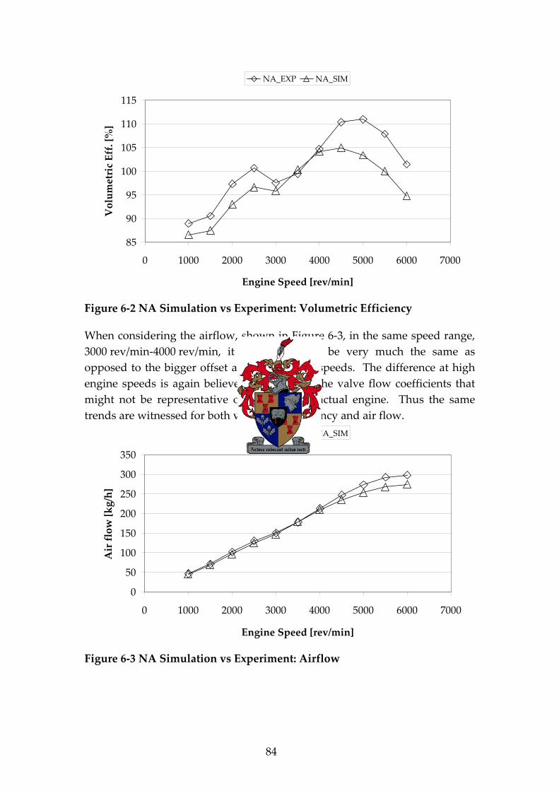
84
85
90
95
100
105
110
115
0 1000 2000 3000 4000 5000 6000 7000
Engine Speed [rev/min]
VolumetricEff.[%]
NA_EXP NA_SIM
Figure 6 2 NA Simulation vs Experiment: Volumetric Efficiency
When considering the airflow, shown in Figure 6 3, in the same speed range,
3000 rev/min 4000 rev/min, it can be seen to be very much the same as
opposed to the bigger offset at higher engine speeds. The difference at high
engine speeds is again believed to be due to the valve flow coefficients that
might not be representative of those on the actual engine. Thus the same
trends are witnessed for both volumetric efficiency and air flow.
0
50
100
150
200
250
300
350
0 1000 2000 3000 4000 5000 6000 7000
Engine Speed [rev/min]
Airflow[kg/h]
NA_EXP NA_SIM
Figure 6 3 NA Simulation vs Experiment: Airflow

85
The fact that the engine simulation predicts more power from the same
amount of airflow could be due to the fact that the simulation does not take
blow by into account. Blow by may not only influence indicated
performance, but also the gas pressure on the rings, which influences the
friction and wear characteristics as well as the hydrocarbon emissions
(Ferguson, 1986). Mass loss due to blow by could then be used to explain the
difference in peak combustion pressures as shown in Figure 6 4. The
maximum difference in peak pressure is 15.4% at 1000 rev/min, with 14.8% at
3500 rev/min.
25
30
35
40
45
50
55
60
65
0 1000 2000 3000 4000 5000 6000 7000
Engine Speed [rev/min]
Max.CombustionPressure[bar]
NA_EXP NA_SIM
Figure 6 4 NA Simulation vs Experiment: Maximum Combustion Pressure
To try and illustrate the effect of blow by, a measured pressure curve for a
motored case is compared in Figure 6 5 to that predicted by simulation. The
difference in peak pressure in the motored case can only be due to blow by
(assuming no measuring error was made), since the air intake pressure,
temperature and airflow through the engine match those of the actual engine.
The difference in motored peak pressure is 14.8%. Using the polytropic
relation Eq 6 1 between volume, pressure and temperature and assuming
isentropic compression with no heat transferred to the gas as it is compressed,
the mass lost due to blow by is 10%. Heywood (1988) states that mass lost
due to blow by is in the order of 1%.
1
2
1
1
1
2
1
2
V
V
P
P
T
T Eq 6 1

86
Using the initial pressure, displacement volume and clearance volume and
assuming no heat transfer from or to the gas, the actual peak pressure for the
motored case is 13.3% lower and the simulation peak pressure is 1.7% higher
than the pressure based on the polytropic relation respectively. The lower
pressure measured in the actual engine can be justified by assuming the
cylinder walls and piston to be at the same temperature as the engine coolant,
thus 90°C, there would certainly be heat loss to the cylinder walls and piston.
The polytropic relation predicts a gas temperature of 425°C at the end of
compression. Thus it is expected that the gas temperature would be lower at
the end of compression due to heat loss and thus resulting in a lower
pressure.
The higher pressure predicted by the simulation can be attributed to the use
of the same boundary conditions as for a fired case. Thus the cylinder walls
and piston would be at a higher temperature than during a motored case and
would cause heat transfer to the gas resulting in a higher temperature and
pressure at the end of compression.
Therefore the discrepancy between the measured and simulated cylinder
pressure could be attributed to a combination of heat addition and
measurement error.
0
500
1000
1500
360 270 180 90 0 90 180 270 360
Crank Angle [°]
Pressure[kPa]
P_EXP P_SIM
Figure 6 5 NA Simulation vs Experiment: Motored in cylinder Pressure
(1500 rev/min)

87
Since the exhaust system is not a complete model representing the actual
exhaust, the orifice can be adjusted in order to give a good correlation
between the exhaust backpressure as predicted and the actual measured data.
This correlation is shown in Figure 6 6.
0
5
10
15
20
25
30
0 50 100 150 200 250 300 350
Mass flow [kg/h]
Exh.BackPress[kPa]
NA_EXP NA_SIM
Figure 6 6 NA Simulation vs Experiment: Exhaust Backpressure
The trend of SFC shown in Figure 6 7 is very much the same; however the
correlation at low engine speeds is better than at high engine speeds. This
could be explained by the combined effect of torque and airflow. At low and
high engine speeds the torque was accurately simulated, but the airflow at
high engine speeds was less accurate than at low and medium engine speeds.
Thus given nearly the same torque at high engine speeds combined with the
lower air flow and thus also lower fuel flow, it directly translates into a lower
SFC.

88
250
270
290
310
330
350
0 1000 2000 3000 4000 5000 6000 7000
Engine Speed [rev/min]
SFC[g/kWh]
NA_EXP NA_SIM
Figure 6 7 NA Simulation vs Experiment: Specific Fuel Consumption
MAP was measured using the engine’s T map sensor. This sensor is used to
measure this engine’s MAP and intake air temperature on the engine. The
data were logged in ETA but were imported from the ECU calibration
software. The resolution of the MAP in the ECU calibration software is very
coarse, which could explain the roughness of the MAP curve in Figure 6 8.
95
96
97
98
99
100
101
102
0 1000 2000 3000 4000 5000 6000 7000
Engine Speed [rev/min]
MAP[kPa]
NA_EXP NA_SIM
Figure 6 8 NA Simulation vs Experiment: Manifold Absolute Pressure

89
The air temperature inside the intake manifold was measured with the T map
sensor. The air temperature in the manifold is not only dependent on the
atmospheric air temperature, but also on the heat transfer from the manifold
itself to the air inside the manifold. The air inside the manifold could heat up
due to radiation and convection from the manifold walls. The effect of this
heating would be more significant at lower engine speeds, when the airflow is
lower and the flow velocity is slower. The air spends more time inside the
manifold before it is induced into the cylinders. This could explain why the
predicted air temperature inside the manifold is much higher than actually
measured at low engine speeds, whereas at higher engine speeds the
correlation is better as is shown in Figure 6 9.
The manifold wall temperature was estimated for the simulations and it was
assumed to be independent of engine speed. Considering the engine is in a
thermal equilibrium condition, it radiates the same amount of heat energy
because it has the same area and the operating temperature should be nearly
the same, because the coolant temperature is controlled to be constant.
Therefore it is assumed that the engine block is at a constant temperature; this
assumption could hold for the intake manifold as well.
25
27
29
31
33
35
37
0 1000 2000 3000 4000 5000 6000 7000
Engine Speed [rev/min]
IntakeManifoldAir
Temperature[°C]
NA_EXP NA_SIM
Figure 6 9 NA Simulation vs Experiment: Intake Manifold Air Temperature

90
This concludes the comparison between the simulated and actual test results
of the NA engine. In general the simulation could predict the trends
accurately, thus the influence that one factor could have on another could be
investigated with the aid of simulations. The maximum error on brake torque
prediction is 8 N m on 131 N m, which equates to 6%. Thus the general
conclusion can be drawn that 1 D flow simulation could be used with
confidence for NA engine performance prediction.
6.2. Turbocharged Results: Simulation versus Experiments
Comparing turbocharged results is not as simple as comparing the naturally
aspirated results, since there are many more factors playing a role and
complicating the comparison. There are various ways of simulating a
turbocharged engine. The way the wastegate is controlled is the main variant.
The wastegate can be operated as a pneumatic valve, opening proportionally
to the boost pressure developed; this method is used on most cars not
equipped with electronic boost control. This proportional control method
was not available in simulation, but by combining a programmed algorithm
with the simulation package it was possible. The other options are specifying
a target BMEP value or boost pressure value that the simulation then tries to
match by opening or closing the wastegate.
For comparison the actual test results will be presented against these three
options: PROP (opening proportional to boost pressure), BMP (target BMEP
value), BP (target boost pressure value). In the proportional case the
wastegate area versus boost pressure in the simulation was adjusted until it
corresponded exactly with that relationship measured on the actual engine.
The torque and power presented for the turbocharged engine are not
corrected, since there is not a standard for correcting the power developed by
a turbocharged SI engine.
The largest error in predicting the torque as shown in Figure 6 10 was the case
where the boost pressure was the same; the predicted torque was more than
the actual with a maximum difference of 17 N m or 9%. The second most
accurate was the proportional control and BMP was exactly the same, which
is expected since the target BMEP was specified for this case. The trends in
torque prediction for all the cases correspond very well.

91
140
150
160
170
180
190
200
210
220
1000 2000 3000 4000 5000 6000
Engine Speed [rev/min]
Torque[Nm]
TRB_EXP PROP_SIM BMP_SIM BP_SIM
Figure 6 10 Turbocharged Simulation versus Experiment: Torque
However, when the boost pressures as shown in Figure 6 11 for the different
cases are compared, the worst prediction was the case where the BMEP was
matched to that of the actual engine. Thus the simulation predicts the same
power output with lower boost pressure or a higher power output with the
same boost pressure. This tendency of the simulation performing better than
the actual engine was witnessed in the NA engine simulation as well
especially between 3000 rev/min and 4500 rev/min where the simulated air
flow was nearly equal to the measured air flow.
1.2
1.25
1.3
1.35
1.4
1.45
1.5
1.55
1.6
1.65
1000 2000 3000 4000 5000 6000
Engine Speed [rev/min]
BoostPressure[bar]
TRB_EXP PROP_SIM BMP_SIM BP_SIM
Figure 6 11 Turbocharged Simulation versus Experiment: Absolute Boost
Pressure

92
Comparing the volumetric efficiencies based on the density in the manifold it
is clear why the actual engine under performs with regards to the torque
developed. It is only at 1500 rev/min and above 4500 rev/min where the
actual engine comes close to the simulation in terms of volumetric efficiency.
At 5000 rev/min and 5500 rev/min the actual engine performs better than the
simulation. As can be seen in Figure 6 13 the actual air flow at 5000 and
5500 rev/min is very similar to the simulation with the same boost pressure.
Thus the actual engine has the same or better volumetric efficiency if the air
flow is similar to that of the simulations.
90
95
100
105
110
115
1000 2000 3000 4000 5000 6000
Engine Speed [rev/min]
VolumetricEfficiency[%]
TRB_EXP PROP_SIM BMP_SIM BP_SIM
Figure 6 12 Turbocharged Simulation vs Experiment: Volumetric Efficiency
When comparing the turbocharged and predicted airflow as shown in Figure
6 13, it can be seen that the airflow is lowest in the BMP case. This is the same
as in the case when comparing the naturally aspirated simulation and test
results; the airflow was lower while developing the same power output. The
PROP case matched the airflow fairly well, but then the predicted torque was
more than the actual torque. In the case where the boost pressure was
matched, the simulation predicted higher airflow than was actually
measured. Thus it can be assumed that the breathing characteristics of the
actual engine and the model used in the simulations are not exactly the same
and this could be attributed to the valve flow coefficients.

93
50
100
150
200
250
300
350
400
450
1000 2000 3000 4000 5000 6000
Engine Speed [rev/min]
Airflow[kg/h]
TRB_EXP PROP_SIM BMP_SIM BP_SIM
Figure 6 13 Turbocharged Simulation versus Experiment: Airflow
The discrepancy between airflow and power developed could partially be due
to blow by, the same as in the naturally aspirated case. The simulation does
not take blow by into account and therefore predicts lower airflow but higher
torque. This could also be used to explain why the predicted maximum
combustion pressures in Figure 6 14 were higher than the actual results,
although the mass lost due to blow by is not significant enough to result in
such a big difference in peak combustion pressure. Therefore factors such as
the accuracy of the spark plug pressure transducer and heat transfer from the
gas inside the cylinder to the cylinder walls could have a significant effect on
the peak combustion pressure.

94
30
40
50
60
70
80
90
1000 2000 3000 4000 5000 6000
Engine Speed [rev/min]
Max.CombustionPressure[bar]
TRB_EXP PROP_SIM BMP_SIM BP_SIM
Figure 6 14 Turbocharged Simulation versus Experiment: Max. Combustion
Pressure
The case where the boost pressure was matched, the maximum combustion
pressure is the highest, but it is also the case where the highest airflow was
predicted. Thus it makes sense that, if a higher mass of air is present in the
combustion chamber, the maximum pressure will also be higher.
However, when comparing the SFC as shown in Figure 6 15, it is interesting
to note the trends of all the different cases are similar and that despite the
difference in boost pressure and developed torque the simulations all predict
the same SFC. The simulated results predicted higher SFC than the actual
engine at low engine speeds and lower SFC at high engine speeds.

95
0.25
0.3
0.35
0.4
0.45
1000 2000 3000 4000 5000 6000
Engine Speed [rev/min]
SFC[kg/kWh]
TRB_EXP PROP_SIM BMP_SIM BP_SIM
Figure 6 15 Turbocharged Simulation versus Experiment: SFC
The intake manifold pressure as shown in Figure 6 16 is dependent on the
boost pressure, but also includes the pressure drop across the intake piping
and throttle. The smallest error was predicted by the BP case, where the boost
pressure was matched exactly. This shows that the flow losses from the
compressor outlet to the intake manifold are representative of the reality. The
largest under prediction was in the case of matching the BMEP, where the
simulation predicted the same power output with a lower boost pressure than
was actually required.
1.2
1.25
1.3
1.35
1.4
1.45
1.5
1.55
1.6
1000 2000 3000 4000 5000 6000
Engine Speed [rev/min]
MAP[bar]
TRB_EXP PROP_SIM BMP_SIM BP_SIM
Figure 6 16 Turbocharged Simulation versus Experiment: MAP

96
Predicting the intake manifold air temperature as shown Figure 6 17, all the
simulations predicted lower temperatures than were actually measured. This
could be due to the fact that the wall temperatures that were used in the
simulations were lower than in reality; thus the air was actually cooled by the
cooler manifold walls.
40
45
50
55
60
65
70
75
80
85
1000 2000 3000 4000 5000 6000
Engine Speed [rev/min]
IntakeManifoldAirTemp.[°C]
TRB_EXP PROP_SIM BMP_SIM BP_SIM
Figure 6 17 Turbocharged Simulation versus Experiment: Intake Manifold
Air Temperature
When comparing the compressor outlet air temperature as shown in Figure
6 18, it is evident that BP was the best prediction. Thus the same increase in
pressure resulted in similar increase in air temperature; therefore the
predicted compressor efficiency should be very close to reality. This indicates
that the simulation interpreted the compressor map correctly and is
representative of the reality. The lower boost pressure as in the case of BMP
results in a lower air temperature; this is further confirmation that the
compressor map and efficiency have been interpreted correctly.

97
50
55
60
65
70
75
80
85
90
95
1000 2000 3000 4000 5000 6000
Engine Speed [rev/min]
CompressorOutletTemperature
[°C]
TRB_EXP PROP_SIM BMP_SIM BP_SIM
Figure 6 18 Turbocharged Simulation versus Experiment: Compressor
Outlet Temperature
The amount of boost pressure developed is proportional to the amount of
energy that can be extracted out of the exhaust gas by the turbine. Thus the
relationship between the wastegate area and boost pressure can be compared
in Figure 6 19 for both the actual and the simulated conditions. It can be seen
that the relationship between the wastegate area and boost pressure is much
more sensitive in the simulated case and therefore the maximum area
predicted is much smaller than was actually measured. It can be seen that the
wastegate area for the PROP case falls on the measured line and thus it was
simulated correctly.

98
0
0.5
1
1.5
2
2.5
3
3.5
1.2 1.3 1.4 1.5 1.6
Boost Pressure [bar]
WastegateArea[cm2]
TRB_EXP PROP_SIM BMP_SIM BP_SIM
Figure 6 19 Turbocharged Simulation versus Experiment: Wastegate Area
What is not obvious immediately when considering Figure 6 19 is why the
wastegate area curves back and thus for the same boost pressure there are two
corresponding area values. This phenomenon occurred in reality as well as in
the simulations. In reality it is impossible to achieve this with the standard
wastegate actuator; since it consist only of a diaphragm and spring, the
opening area must be proportional to the boost pressure. The cause of this
effect is the force on the wastegate valve itself due to the large pressure
difference between the turbine entry and outlet. Thus the force experienced
by the spring is the sum of the force on the diaphragm caused by the boost
pressure and the force on the wastegate valve caused by the pressure
difference across it. Thus the force on the wastegate valve causes the
wastegate to open more than is predicted by using purely the boost pressure.
When considering the wastegate area versus exhaust mass flow, as shown in
Figure 6 20, it is interesting to note that it is a near linear relationship. The
gradient of the actual results is totally different from that predicted by the
simulation. Thus it can be concluded that the wastegate area and or its flow
characteristics were not simulated correctly or the calculation of the wastegate
area from the measured rack travel is inaccurate.

99
0
0.5
1
1.5
2
2.5
3
3.5
0 100 200 300 400 500
Mass Flow [kg/h]
WastegateArea[cm2]
TRB_EXP PROP_SIM BMP_SIM BP_SIM
Figure 6 20 Turbocharged Simulation versus Experiment: Wastegate Area as
function of mass flow
In Figure 6 21 the turbine pressure ratio which best resembles the actual
results is that of the BMP case. The pressure ratios for the other cases were
both higher. This is due to the fact that the predicted turbine inlet pressure
was higher for the same mass flow than the actual results indicated. This
complements the assumption that the flow characteristic of the simulated
turbine does not correspond to the actual tests.
1.1
1.2
1.3
1.4
1.5
1.6
1.7
1.8
1000 2000 3000 4000 5000 6000
Engine Speed [rev/min]
TurbinePressureRatio(Pin/Pout)
TRB_EXP PROP_SIM BMP_SIM BP_SIM
Figure 6 21 Turbocharged Simulation versus Experiment: Turbine Pressure
Ratio

100
The predicted turbine inlet temperature as shown in Figure 6 22 correlated
fairly well. The temperatures are predicted well inside the range of the 50°C
error, which is the sort of error that can be expected when measuring exhaust
temperatures as is done in practice (see section 5.7.3). What is a matter of
concern is that the predicted temperatures are lower than the actual results.
The measuring error would cause thermocouple readings that are lower than
the actual values. Thus the predicted result should have been higher.
700
750
800
850
900
950
1000 2000 3000 4000 5000 6000
Engine Speed [rev/min]
TurbineInletTemperature[°C]
TRB_EXP PROP_SIM BMP_SIM BP_SIM
Figure 6 22 Turbocharged Simulation versus Experiment: Turbine Inlet
Temperature
However, the fact that the simulation predicts lower temperatures only at
speeds above 2500 rev/min could be linked to the fact that very rich mixtures
were used at speeds above 2500 rev/min. Thus the simulation predicts lower
exhaust temperatures than the actual temperatures, especially when very rich
mixtures were used. A possible reason for this is the simulation’s inability to
accurately predict exhaust temperature with very rich mixtures. Another
possibility could be that there might have been combustion in the exhaust
manifold if air was leaking into the exhaust manifold. The air could be
introduced into the exhaust manifold, although the exhaust manifold pressure
was nominally higher than the atmospheric pressure; due to the pulsation
effects in the exhaust manifold.

101
It can be concluded that the simulated results showed the same trends as were
measured on the actual engine. The compressor modelling seems to be of a
high standard, but there is concern about turbine modelling and map
interpretation as well as the wastegate area predicted. The engine power
output is highly dependent on the boost pressure, which is in turn dependent
on the energy extracted from the exhaust gas. Thus both the compressor and
turbine modelling should be accurate in order to predict the same boost
pressure, turbine inlet pressure as well as wastegate area.
6.3. Comparison of the NA and Turbocharged Results
When comparing the turbocharged engine to the NA engine, not only are the
same aspects considered as in the previous two sections, but the forces on the
bearings and the energy balance were also compared. The forces are an
important factor, because if the forces developed exceed the functional limit of
the components, then durability will be compromised. The energy balance
can be used to audit the modifications made to the engine in order to make an
objective engineering judgement whether it is worthwhile.
The CR of the turbocharged engine was the same as that of the NA engine
and the turbocharged engine did not have an intercooler. Thus the
compressor would increase both the initial charge pressure and temperature
and knock could result. Therefore a fuel with a higher octane was used
during the turbocharged engine tests. The fuel used was Shell 102.6 octane
racing fuel. This fuel contains more than 0.05% lead and can therefore be
classified as leaded. The fuel used during testing of the NA engine was
unleaded with a 95 RON.
6.3.1. Comparison of Turbocharged Boost Settings
Different wastegate actuator settings were tested in order to find the best
solution that would give a torque curve as flat as possible while producing a
maximum of 100 kW. The experiments were started at low boost and the
boost pressure was gradually increased until the 100 kW target was reached.
In this section only the different boost pressures, lambda settings, ignition
timing, compressor operating points and the resulting torque curves will be
compared to the NA engine. A detailed comparison involving only the
optimum boost setting and the NA engine results will follow in the next
section.

102
The boost pressures (gauge) developed are shown in Figure 6 23. The NA
engine has no boost pressure and is therefore 0 bar. The lowest boost curve,
0.21 bar, was run with the NA engine’s standard exhaust pipe. This caused a
very high exhaust backpressure and it was then replaced with a free flow
exhaust. A peak boost pressure of 0.21 bar was achieved with no preload on
the spring in the variable wastegate actuator. Due to the stiffness of the
diaphragm, the same spring stiffness was used in all the tests. The standard
wastegate actuator was used in the 0.36 bar STD experiment, and the preload
was set so that the wastegate would start opening at 0.3 bar boost. As can be
seen, this is the flattest boost curve, because this actuator opens linearly with
boost pressure. The highest boost curve was the one that was actually used,
since it met the target power output.
0
0.1
0.2
0.3
0.4
0.5
0.6
1500 2000 2500 3000 3500 4000 4500 5000 5500 6000
Engine Speed [rev/min]
BoostPressure[bar]
0.58bar 0.55bar 0.44bar 0.36bar_STD 0.21bar NA
Figure 6 23 Turbocharged Boost Settings: Boost Pressure
The lambda settings for the experiments are shown in Figure 6 24. It is
evident that the NA engine’s lambda was the closest to stoichiometric. The
turbocharged engine’s exhaust temperatures were very high and therefore a
very rich lambda was used to maintain port temperatures below the threshold
of 830 C.

103
0.7
0.75
0.8
0.85
0.9
0.95
1500 2000 2500 3000 3500 4000 4500 5000 5500 6000
Engine Speed [rev/min]
Lambda
0.58bar 0.55bar 0.44bar 0.36bar_STD 0.21bar NA
Figure 6 24 Turbocharged Boost Settings: Lambda
The ignition timing is compared in Figure 6 25. As can be seen, the ignition
timing was most advanced in the 0.21 bar experiment. This was possible
since the boost pressure was low and high octane fuel was being used,
therefore knock was not a limitation. As the boost pressure was increased, the
ignition timing had to be retarded, since knock became a limitation.
10
12
14
16
18
20
22
24
26
28
30
1500 2000 2500 3000 3500 4000 4500 5000 5500 6000
Engine Speed [rev/min]
IgnitionTiming[CABTDC]
0.58bar 0.55bar 0.44bar 0.36bar_STD 0.21bar NA
Figure 6 25 Turbocharged Boost Settings: Ignition Timing

104
The compressor operating points were superimposed on the compressor map
and this compressor map is shown in Figure 6 26. Since the NA engine did
not have a compressor, its operating points are only shown in order to see the
difference in volume flow rates. It can be seen that 0.58 bar runs through the
highest efficiency area of the compressor. Therefore the match between the
compressor and this engine is very good.
57000
87000
118000
140000
160000
175000
187000
0.72
0.71
0.7
0.68
0.68
0.65
0.6
0.650.6
0.55
1.0
1.2
1.4
1.6
1.8
2.0
2.2
2.4
2.6
2.8
0.00 0.02 0.04 0.06 0.08 0.10 0.12 0.14 0.16
Volume flow [m^3/s]
PressureRatio[P2t/P1t]
0.58bar 0.55bar 0.44bar 0.36bar_STD 0.21bar NA
Figure 6 26 Turbocharged Boost Settings: Compressor Operating Points
The torque curves for the different boost settings are shown in Figure 6 27.
The higher the boost pressure the higher the torque produced. It is evident
from all the curves that the torque decreases considerably at engine speeds
higher than 4000 rev/min. When considering the boost curve of 0.36 bar STD,
it is nearly flat from 2000 rev/min up to 5500 rev/min. This boost curve
resulted in a very flat torque curve from 2500 rev/min up to 4000 rev/min,
after which it decreases significantly. Therefore more boost is needed at high
engine speeds in order to maintain the same amount of torque.
This phenomenon of decreasing torque can partly be due to the fact that at
4000 rev/min the compressor is at its highest efficiency; thus at higher engine
speeds the boost pressure drops and the boost temperature increases.
Another factor that could cause the torque to decrease at engine speeds higher
than 4000 rev/min is pulse interference. Pulse interference was discussed in a
previous section (5.1.1) and it could be very engine speed specific (Watson &
Janota, 1984). It impedes the gas exchange process and causes higher residual
mass in the combustion chamber. Therefore the torque produced would be
less.

105
120
140
160
180
200
220
1500 2000 2500 3000 3500 4000 4500 5000 5500 6000
Engine Speed [rev/min]
Torque[Nm]
0.58bar 0.55bar 0.44bar 0.36bar_STD0.21bar NA 100 kW
Figure 6 27 Turbocharged Boost Settings: Torque
Different boost settings were tested and the resulting torque curves were
presented. The boost curve with the highest boost resulted in the highest
power output and the 100 kW target was reached with this setting at
5000 rev/min. In the following discussions all the turbocharged results refer
to the 0.58 bar boost setting.
6.3.2. Force Analysis
An important aspect of engine analysis is the loading on the bearings. Since
the in cylinder pressure was measured, the forces on the piston can be
calculated. The acceleration forces, however, are not explicitly known, but
assumptions can be made to make calculations simpler. The assumptions can
be summarised as follows:
The crankshaft is turning at a constant speed;
The piston’s centre of mass is at the centre of the small end
bearing;
The connecting rod is composed of two point masses, one at
each end, connected with a weightless rod;
The crankshaft is perfectly balanced and it is assumed to be
weightless;
Friction is neglected in all joints as well as between the piston
and cylinder wall.

106
The mass of a generic piston and connecting rod was used. Therefore the
forces quoted in this comparison cannot be used as absolute values. The
objective was to investigate the order of magnitude of the bearing forces that
an increase in cylinder pressure would have.
A pure mathematical model was derived for the motion (displacement,
velocity and acceleration) of the piston. The derived equations can be seen in
APPENDIX D. The method of dynamically equivalent masses as described by
Mabie, H H and Reinholtz, C F (1987) was used to account for the inertia of
the connecting rod. The mass of the counter weights was chosen so that they
would perfectly balance the mass of the connecting rod at the big end bearing.
An elementary model of the crank, connecting rod and piston was also built
in Adams View to compare it to the mathematical model. The gas force on
the piston, as a function of crank angle, and the rotational speed of the
crankshaft was used as input to the simulation. The simulation then animates
movement and calculates the accelerations and forces at the bearings. These
accelerations can then be compared to those of the mathematical model for
correlation. Figure 6 28 show the correlation between the piston’s
acceleration and velocity calculated by the derived mathematical equations
and the simulation.
25000
20000
15000
10000
5000
0
5000
10000
15000
0 90 180 270 360 450 540 630 720
Crank Angle [°]
Acceleration[m/s2]
30
20
10
0
10
20
30
Velocity[m/s]
Piston Acc. Sim Acc. Piston Vel. Sim Vel.
Figure 6 28 Piston Velocity and Acceleration Correlation
The correlation between the analytical and simulated magnitude of the force
in the small and big end bearings of the NA engine at 3000 rev/min and
WOT are presented in Figure 6 29 and Figure 6 30 respectively and the
correlation was very good.
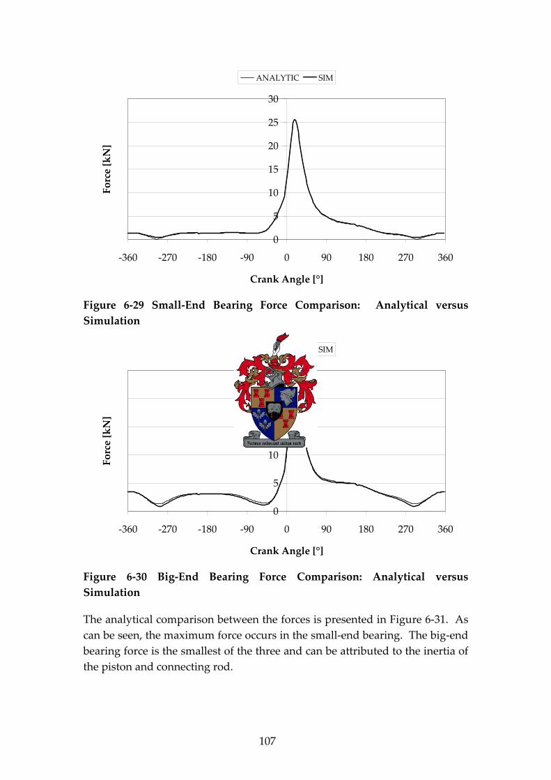
107
0
5
10
15
20
25
30
360 270 180 90 0 90 180 270 360
Crank Angle [°]
Force[kN]
ANALYTIC SIM
Figure 6 29 Small End Bearing Force Comparison: Analytical versus
Simulation
0
5
10
15
20
25
360 270 180 90 0 90 180 270 360
Crank Angle [°]
Force[kN]
ANALYTIC SIM
Figure 6 30 Big End Bearing Force Comparison: Analytical versus
Simulation
The analytical comparison between the forces is presented in Figure 6 31. As
can be seen, the maximum force occurs in the small end bearing. The big end
bearing force is the smallest of the three and can be attributed to the inertia of
the piston and connecting rod.

108
The inertia force is always in the opposite direction to the acceleration, and
therefore the inertia force acting on the big end bearing can be subtracted
from the gas force acting on the piston. This is the reason why the big end
bearing’s maximum force is smaller than that of the small end bearing. A
similar reasoning can be used to explain the difference between the main
bearing and small and big end bearing forces. The force on the main bearing
is carried by two bearings in the case of a single cylinder engine. In the case
of a multiple cylinder engine depending on engine configuration, the main
bearing forces of two adjacent cylinders always cause negative interference
and tend to cancel each other out.
0
5
10
15
20
25
30
360 270 180 90 0 90 180 270 360
CA [°]
Force[kN]
Small Big Main
Figure 6 31 Analytically Determined Bearing Forces
The forces predicted by the simulation are only a magnitude (do not take the
direction of action into account) and therefore only the maximum forces for
the NA engine and turbocharged engine will be compared. The gas force that
acts on top of the piston is presented in Figure 6 32. The drop in gas force at
5000 rev/min is due to the late ignition timing and longer burn duration. The
maximum gas pressure for the turbocharged engine occurred 5°CA later at
5000 rev/min than at the other engine speeds. The burn rate at 5000 rev/min
was also 5°CA slower than the average of other speeds.

109
10
15
20
25
30
35
40
1000 2000 3000 4000 5000 6000 7000
Engine Speed [rev/min]
Force[N]
Fgas_NA Fgas_TRB
Figure 6 32 NA versus Turbocharged Results: Gas Force on Piston
The maximum forces on the small and big end bearings at different engine
speeds are presented in Figure 6 33 and Figure 6 34 respectively. When
considering the gas force in the NA engine, it is fairly constant from
3000 rev/min up to 6000 rev/min; however, the small and big end bearing
forces decrease with an increase in engine speed. This is due to the fact that
as the engine speed increases, the inertia force also increases and, as explained
earlier, the inertia force tends to cancel out the gas force on the piston.
Therefore the force on the bearings decreases as the engine speed increases
and the gas pressure remains nearly constant.
The same reasoning can be followed for the turbocharged engine; however,
the gas pressure does not decrease, but increases steadily with increased
engine speeds, yet the bearing forces still decrease as the engine speed
increases.

110
10
15
20
25
30
35
40
1000 2000 3000 4000 5000 6000 7000
Engine Speed [rev/min]
Force[kN]
Fsmall_NA Fsmall_TRB
Figure 6 33 NA versus Turbocharged Results: Small end Bearing Forces
The forces on the small end bearings are higher than those on the big end due
to the mass and inertia of the connecting rod. Due to the simplification
assumptions the forces predicted by simulation on the main bearings are
exactly equal to those on the big end bearings and are therefore not
presented.
10
15
20
25
30
35
40
1000 2000 3000 4000 5000 6000 7000
Engine Speed [rev/min]
Force[kN]
Fbig_NA Fbig_TRB
Figure 6 34 NA versus Turbocharged Results: Big end Bearing Forces

111
The maximum forces on both the small and big end bearings were increased
by 45% and 49% respectively as a result of turbocharging to yield 48% more
torque and 37% more power. The area under the curves was also increased;
thus it could be assumed that the turbocharged engine is more susceptible to
failure due to fatigue as a result of the increased loading and thus a
compromise on durability is inevitable.
6.3.3. Energy Balance
Energy cannot be created nor be destroyed; thus if energy enters a system,
and the energy of the system does not increase, it must leave the system.
Thus an energy balance is the sum of what enters, what leaves and what
remains in the system. If the system is in a steady state condition, its energy
(or temperature) can be assumed to remain constant, and then it is only
necessary to consider what enters and what leaves the system.
The simplification was made that air at atmospheric conditions has zero
potential energy; thus the exhaust gases have a great deal of thermal energy.
Thus the amount of energy input into the system in terms of fuel energy must
be recovered as shaft energy, heat rejected to the cooling system, thermal
energy in exhaust gas, chemical energy in the exhaust gas and radiation to the
surroundings. The chemical energy in the exhaust is made up of partially and
un burnt hydrocarbons and carbon monoxide. The energy in the carbon
monoxide can be accounted for with a relation presented by Heywood (1988).
The hydrocarbons are unaccounted for and make up part of “other” energy.
Due to the complicated measurement of radiation energy, it is also accounted
for as “other” energy.
The heat rejection was measured by installing 2 orifice flow meters; one in the
engine’s cooling system and the other in the facility water side that circulated
through the oil cooler. The engine coolant was thus not routed through the
oil cooler in order to measure the effect of the turbocharger on the oil
separately from that of the cooling system. The pressure drop across the
orifices was measured as well as the temperature difference across the engine
and oil cooler. From these measurements the mass flow and thus the total
energy removed could be calculated. The heat rejected to the cooling system,
which uses a mixture of 50% water and 50% ethylene glycol can be calculated
if the specific heat for the fluid are known. The specific heat value was
extrapolated by fitting a second order polynomial to the data found in Mills
(1995), see Figure 6 35. The specific heat at 90°C was found to be 3786 J/kg K
compared to a specific heat value of 4128 J/kg K for pure water.

112
y = 0.0053571x2 0.5178571x + 3268.3928571
R2= 0.9914273
3400
3500
3600
3700
3800
3900
4000
250 275 300 325 350 375 400
Temperature [K]
SpecificHeat[J/kg.K]
Aqueous Ethylene Glycol Solution
Figure 6 35 Extrapolation of Specific Heat
When comparing the heat rejected to the cooling system and the oil cooler as
shown in Figure 6 36, the heat rejected to the cooling system is more in the
case of the turbocharged engine, as can be expected, but what is of interest is
that the heat removed by the oil cooler is nearly the same.
The maximum increase in heat rejected to the cooling system was 35% which
is in the same order of magnitude as the 37% increase in maximum power
output. Therefore it can be assumed that, if the power output of an SI engine
is increased by x%, the cooling system would have an x% increased loading
and should be upgraded if it does not have enough spare capacity.

113
0
5
10
15
20
25
30
35
40
1000 2000 3000 4000 5000 6000
Engine Speed [rev/min]
HeatRejection[kW]
NA_coolant TRB_Coolant NA_Oilcooler TRB_Oilcooler
Figure 6 36 NA versus Turbocharged Results: Heat Rejection
It might be considered that the oil cooler is operating at its limit and therefore
no more heat can be extracted, but when looking at the oil temperature as
shown in Figure 6 37, it can be seen that the oil temperature of the
turbocharged engine is actually lower than for the NA engine. This can be
explained by the fact that the turbocharger’s bearing housing is water cooled.
Thus most of the heat energy in the bearing housing is removed by the
cooling system and not the oil; in fact some of the heat energy in the oil must
be removed by the cooling system, because the oil temperature is lower for
the turbocharged engine.

114
80
85
90
95
100
105
110
115
120
125
1000 2000 3000 4000 5000 6000
Engine Speed [rev/min]
OilTemperature[°C]
NA_EXP TRB_EXP
Figure 6 37 NA versus Turbocharged Results: Oil Temperature
When comparing the energy balance for the NA engine in Figure 6 38 to that
of the turbocharged engine in Figure 6 39, it must be kept in mind that
everything is in percentages and that 100% of the fuel energy for the NA
engine is actually less than 100% for the turbocharged engine because of the
different fuel quantities consumed.
It is interesting to note that the NA engine never converted less than 25% of
the fuel energy into shaft energy, as opposed to the turbocharged engine,
which at 5000 rev/min and 5500 rev/min is only converting 20% of the fuel
into useful shaft energy. This is due to the fact that a very rich mixture was
used to cool down the exhaust temperatures. What is a matter of concern is
the fact that the “other” energy accounts for 38% to 46% of the fuel energy in
the case of the turbocharged engine from 3000 rev/min to 5500 rev/min. This
is due to the fact that unburned and partially burned fuel is leaving through
the exhaust, which is unaccounted for in the energy balance. When operating
at part load with lambda values near 1, the amount of “other” energy
decreases drastically to about 6% to 10% of the fuel energy. This is shown and
explained in section 6.3.5. The chemical energy contained in the carbon
monoxide accounts for a maximum of 2% in the case of the NA engine and 3%
for the turbocharged engine.

115
27.2 29.5 29.7 31.2 29.3 27.5 27.6 26.5 25.4
23.0 21.2 19.8 19.117.5
15.9 16.1 15.6 15.2
18.8 22.2 22.4 23.923.7
23.7 25.8 25.2 26.0
29.6 25.7 26.6 24.2 27.9 31.0 28.7 30.8 31.3
0%
20%
40%
60%
80%
100%
1500 2000 2500 3000 3500 4000 4500 5000 5500
Engine Speed [rev/min]
FuelEnergy[%]
%Shaft Work %Cooling %Exhaust %Other %CO Exh.
Figure 6 38 NA engine: Energy Balance at WOT
When comparing the percentage of energy leaving the exhaust, it can be seen
that about 5% more goes to waste in the NA engine than in the turbocharged
engine. This is where it is beneficial to have a turbine that utilises some of the
energy that is available in the exhaust gas.
27.7 30.9 29.9 27.1 26.7 25.7 24.7 20.7 21.1
26.8 21.017.7
14.7 13.7 12.5 12.110.0 10.8
19.3 20.720.3
19.0 19.8 20.4 21.7
19.8 20.9
24.6 26.030.5
37.2 37.6 38.9 38.946.4 44.3
0%
20%
40%
60%
80%
100%
1500 2000 2500 3000 3500 4000 4500 5000 5500
Engine Speed [rev/min]
FuelEnergy[%]
%Shaft Work %Cooling %Exhaust %Other %CO Exh.
Figure 6 39 Turbocharged Engine: Energy Balance at WOT

116
6.3.4. Performance Comparison
Before the turbocharged conversion was done, the base engine was tested to
have a baseline for comparison. After all the testing on the turbocharged
engine was completed, the engine was built back to the original specification
in order to see whether the engine sustained any damage or performance
degradation. The torque measured before and after the conversion is
presented in Figure 6 40. It can be seen that there are no major differences;
thus it would be safe to assume that the engine has not suffered any damage
because its performance is on par. This also gives an indication of the
repeatability of the test procedure and reliability of the equipment used.
105
110
115
120
125
130
135
140
0 1000 2000 3000 4000 5000 6000 7000
Engine Speed [rev/min]
CorrectedTorque[Nm]
Pre_Conversion Post_Conversion
Figure 6 40 NA Engine Torque
The measured torque and power of the turbocharged and NA engine are
shown in Figure 6 41. The torque was increased at 1500 rev/min with 27 N m.
The maximum increase in torque is at 4000 rev/min, where it is increased by
64 N m, which translates to an increase of 48%. The maximum power output
was increased by 37% to a maximum of 96 kW.
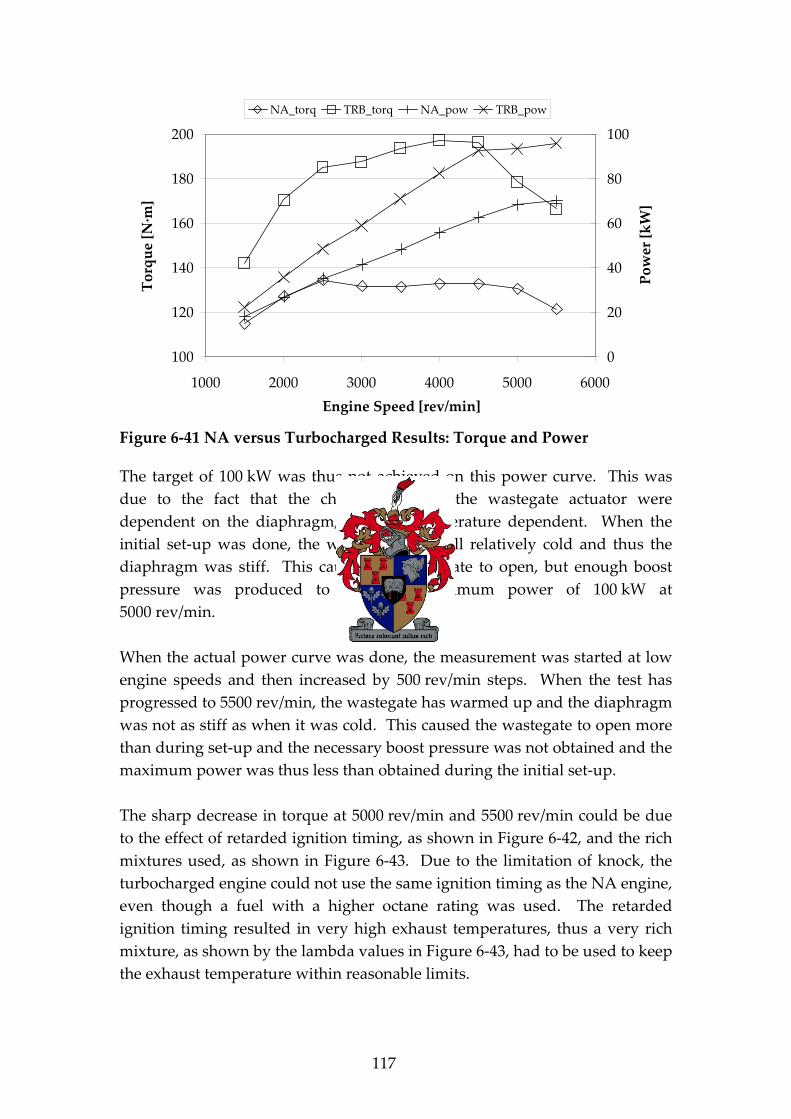
117
100
120
140
160
180
200
1000 2000 3000 4000 5000 6000
Engine Speed [rev/min]
Torque[Nm]
0
20
40
60
80
100
Power[kW]
NA_torq TRB_torq NA_pow TRB_pow
Figure 6 41 NA versus Turbocharged Results: Torque and Power
The target of 100 kW was thus not achieved on this power curve. This was
due to the fact that the characteristics of the wastegate actuator were
dependent on the diaphragm, which is temperature dependent. When the
initial set up was done, the wastegate was still relatively cold and thus the
diaphragm was stiff. This caused the wastegate to open, but enough boost
pressure was produced to obtain a maximum power of 100 kW at
5000 rev/min.
When the actual power curve was done, the measurement was started at low
engine speeds and then increased by 500 rev/min steps. When the test has
progressed to 5500 rev/min, the wastegate has warmed up and the diaphragm
was not as stiff as when it was cold. This caused the wastegate to open more
than during set up and the necessary boost pressure was not obtained and the
maximum power was thus less than obtained during the initial set up.
The sharp decrease in torque at 5000 rev/min and 5500 rev/min could be due
to the effect of retarded ignition timing, as shown in Figure 6 42, and the rich
mixtures used, as shown in Figure 6 43. Due to the limitation of knock, the
turbocharged engine could not use the same ignition timing as the NA engine,
even though a fuel with a higher octane rating was used. The retarded
ignition timing resulted in very high exhaust temperatures, thus a very rich
mixture, as shown by the lambda values in Figure 6 43, had to be used to keep
the exhaust temperature within reasonable limits.

118
0
5
10
15
20
25
30
1000 2000 3000 4000 5000 6000
Engine Speed [rev/min]
SparkAdvance[°CABTDC]
NA_EXP TRB_EXP
Figure 6 42 NA versus Turbocharged Results: Ignition Timing
During a telephonic interview with a calibration engineer, P Krabbendam
(2004), who was involved with the initial calibration of the ECU on the
standard production engine, the limit on exhaust port temperature was
mentioned as 815 °C. This limit was due to the specific exhaust valves and
valve seats being used in these engines.
0.6
0.65
0.7
0.75
0.8
0.85
0.9
0.95
1000 2000 3000 4000 5000 6000
Engine Speed [rev/min]
Lambda
NA_EXP TRB_EXP
Figure 6 43 NA versus Turbocharged Results: Lambda

119
As a result of the retarded ignition timing and very rich mixtures, the
turbocharged engine operated at a higher SFC than the NA engine, as shown
in Figure 6 44. The lower the SFC the more efficient the engine. The highest
SFC values were at 5000 rev/min and 5500 rev/min, where the lambda values
were below 0.75. The turbocharged engine operated at lower SFC than the
NA engine at engine speeds below 2500 rev/min. At these operating
conditions the ignition timing was nearly the same, but the lambda was
slightly richer than that of the NA engine. Thus the higher power output at
these low engine speeds resulted in an SFC below that of the NA engine.
200
250
300
350
400
450
1000 2000 3000 4000 5000 6000
Engine Speed [rev/min]
SFC[g/kWh]
NA_EXP TRB_EXP
Figure 6 44 NA versus Turbocharged Results: SFC
The intake manifold absolute pressure, MAP, and intake manifold
temperature, TMAP (measured with TMAP sensor), are shown in Figure 6 45.
This indicates that the difference in MAP between the turbocharged and NA
engine is nearly 60 kPa. The temperature difference between the two versions
of the engine is about 50°C above 5000 rev/min. The boost pressure decreases
slightly from 4000 rev/min and higher. This reduction in boost pressure can
be attributed to the force on the wastegate valve caused by the pressure drop
across the valve. Thus the wastegate opens more and less boost pressure is
developed.

120
0
20
40
60
80
100
120
140
160
180
200
1000 2000 3000 4000 5000 6000
Engine Speed [rev/min]
IntakeManifoldPressure[kPa]
0
10
20
30
40
50
60
70
80
90
100
IntakeManifoldTemperature
[°C]
NA_MAP TRB_MAP NA_TMAP TRB_TMAP
Figure 6 45 NA versus Turbocharged Results: MAP and TMAP
The boost pressure versus wastegate area is shown in Figure 6 46. It can be
seen that the wastegate opens more for the same boost pressure when the area
is bigger than 2.5 cm2. This was phenomenon was explained in a previous
section (p 98).
0
0.5
1
1.5
2
2.5
3
3.5
1 1.1 1.2 1.3 1.4 1.5 1.6
Boost Pressure [bar]
WastegateArea[cm2]
TRB_EXP
Figure 6 46 NA versus Turbocharged Results: Wastegate Area

121
The increased pressure in the manifold resulted in a higher density in the
manifold, as shown in Figure 6 47. The effect of decreasing boost pressure
and increasing temperature is clearly visible on the air density inside the
intake manifold of the turbocharged engine for engine speeds above
4000 rev/min. On the NA engine a similar phenomenon is witnessed, and this
is due to the increase in temperature and the decrease in MAP. MAP drops as
speed increases due to the upstream restrictions including the clean air
system (filter, pipes and throttle body).
1
1.1
1.2
1.3
1.4
1.5
1.6
1.7
1000 2000 3000 4000 5000 6000
Engine Speed [rev/min]
AirDensity[kg/m
3]
NA_EXP TRB_EXP
Figure 6 47 NA versus Turbocharged Results: Intake Manifold Air Density
The increase in TMAP for the NA engine is due to the ambient air
temperature, as shown in Figure 6 48, which increased during the duration of
the test. The ambient temperature increased, since the test cell did not have
controlled air temperature.
The temperature increase from ambient to TMAP for the turbocharged engine
is due to the compression of the air through the compressor. If an intercooler
had been installed, the TMAP could have been reduced. This would have had
a major effect on the density, since density is inversely proportional to
temperature. Thus it would have been possible to develop the same amount
of torque with a lower boost pressure. If a moderate temperature difference
of 30°C could be achieved across the intercooler, it would be possible to
obtain the same density with a decrease of 9% on boost pressure, thus the
boost pressure could be lowered to about 0.43 bar instead of 0.58 bar (gauge).
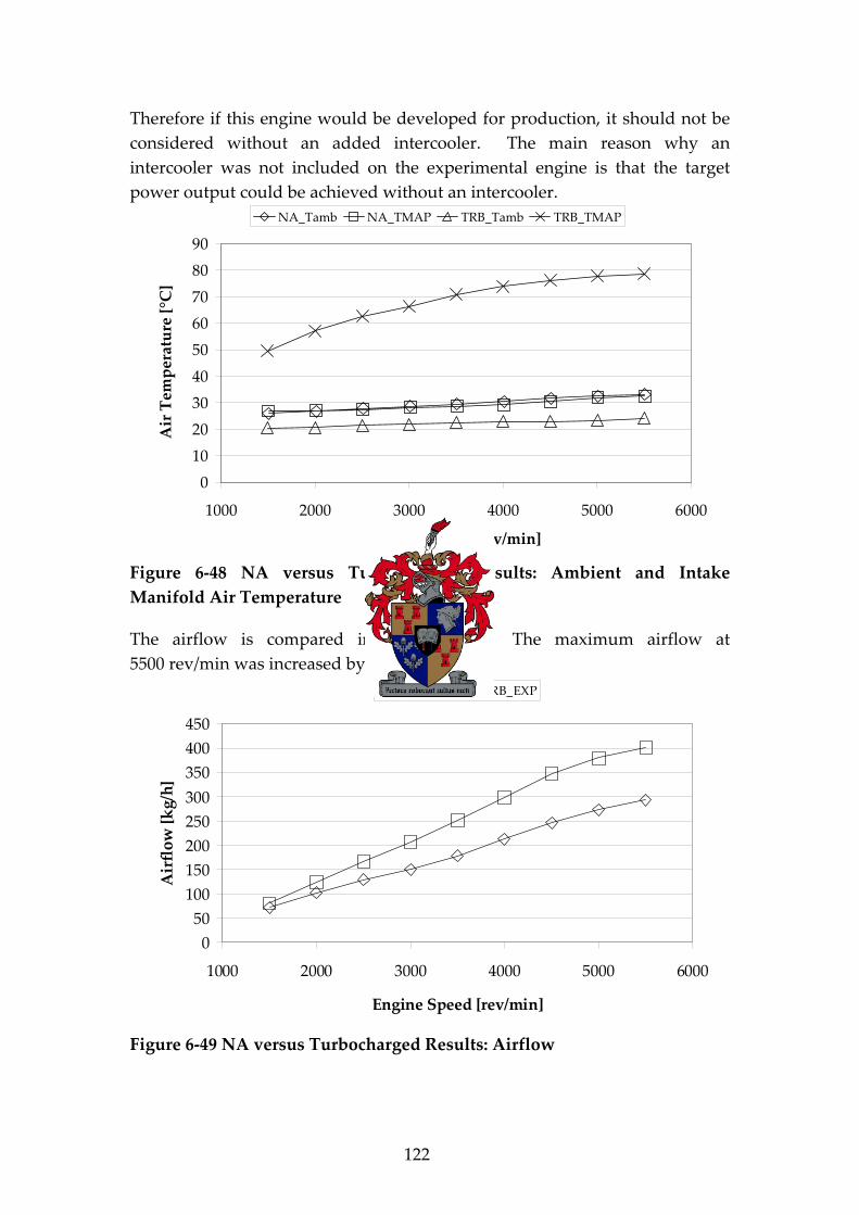
122
Therefore if this engine would be developed for production, it should not be
considered without an added intercooler. The main reason why an
intercooler was not included on the experimental engine is that the target
power output could be achieved without an intercooler.
0
10
20
30
40
50
60
70
80
90
1000 2000 3000 4000 5000 6000
Engine Speed [rev/min]
AirTemperature[°C]
NA_Tamb NA_TMAP TRB_Tamb TRB_TMAP
Figure 6 48 NA versus Turbocharged Results: Ambient and Intake
Manifold Air Temperature
The airflow is compared in Figure 6 49. The maximum airflow at
5500 rev/min was increased by 37% to 400 kg/h.
0
50
100
150
200
250
300
350
400
450
1000 2000 3000 4000 5000 6000
Engine Speed [rev/min]
Airflow[kg/h]
NA_EXP TRB_EXP
Figure 6 49 NA versus Turbocharged Results: Airflow

123
When considering the volumetric efficiency, which is based on the manifold
conditions, as shown in Figure 6 50, the NA engine has a higher volumetric
efficiency below 2500 rev/min than the turbocharged engine. Above
2500 rev/min the higher air density increases the volumetric efficiency of the
turbocharged engine above that of the NA engine.
80
85
90
95
100
105
110
115
1000 2000 3000 4000 5000 6000
Engine Speed [rev/min]
VolumetricEfficiency[%]
NA_EXP TRB_EXP
Figure 6 50 NA versus Turbocharged Results: Volumetric Efficiency
When considering the exhaust manifold pressure as shown in Figure 6 51, it
can be seen that the turbine causes a very large backpressure.
0
20
40
60
80
100
120
1000 2000 3000 4000 5000 6000
Engine Speed [rev/min]
ExhaustManifoldPressure[kPa]
NA_EXP TRB_EXP
Figure 6 51 NA versus Turbocharged Results: Exhaust Manifold Pressure

124
To put the exhaust manifold pressure into perspective, let us consider the
pressure difference between the intake and exhaust manifold. This pressure
difference is shown in Figure 6 52. The turbocharged engine’s pressure
difference is positive at engine speeds below 2500 rev/min. This is also the
range where a lower SFC was recorded for the turbocharged engine. Thus
above 2500 rev/min the engine does pumping work, which might seem
contradicting to the principle of turbocharging. Due to the boost limitation on
spark ignition engines this will always be witnessed for especially engines
fitted with a small turbocharger to improve the engines response. On large
compression ignition engines, it would be expected that there is always a
positive pressure difference across the engine if it is a well designed system
(Watson & Janota, 1984).
60
40
20
0
20
1000 2000 3000 4000 5000 6000
Engine Speed [rev/min]
PressureDifference[kPa]
NA_EXP TRB_EXP
Figure 6 52 NA versus Turbocharged Results: Pressure Difference (Intake
Manifold Exhaust Manifold)
The exhaust backpressure (post turbine) is plotted as a function of mass flow,
the sum of fuel flow and airflow, in Figure 6 53. This is where the advantage
of the free flow exhaust is evident. The measured exhaust backpressures are
about the same, but they occur at very different mass flow rates. Therefore
the free flow exhaust system can handle more mass flow while producing the
same backpressure as the standard exhaust system.
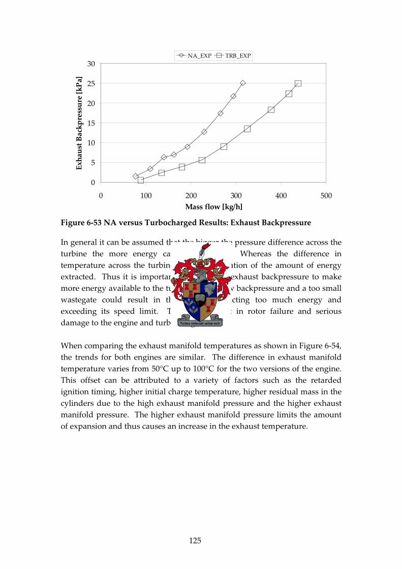
125
0
5
10
15
20
25
30
0 100 200 300 400 500
Mass flow [kg/h]
ExhaustBackpressure[kPa]
NA_EXP TRB_EXP
Figure 6 53 NA versus Turbocharged Results: Exhaust Backpressure
In general it can be assumed that the bigger the pressure difference across the
turbine the more energy can be extracted. Whereas the difference in
temperature across the turbine gives an indication of the amount of energy
extracted. Thus it is important to reduce the exhaust backpressure to make
more energy available to the turbine. A too low backpressure and a too small
wastegate could result in the turbine extracting too much energy and
exceeding its speed limit. This could result in rotor failure and serious
damage to the engine and turbocharger.
When comparing the exhaust manifold temperatures as shown in Figure 6 54,
the trends for both engines are similar. The difference in exhaust manifold
temperature varies from 50°C up to 100°C for the two versions of the engine.
This offset can be attributed to a variety of factors such as the retarded
ignition timing, higher initial charge temperature, higher residual mass in the
cylinders due to the high exhaust manifold pressure and the higher exhaust
manifold pressure. The higher exhaust manifold pressure limits the amount
of expansion and thus causes an increase in the exhaust temperature.

126
550
600
650
700
750
800
850
900
950
1000 2000 3000 4000 5000 6000
Engine Speed [rev/min]
Temperature[°C]
NA_EXP TRB_EXP Post_TRB
Figure 6 54 NA versus Turbocharged Results: Exhaust Manifold
Temperature
Post turbine temperatures are on average 30°C lower than the NA exhaust
manifold temperatures. The difference between pre and port turbine
temperatures decreases with increasing engine speed. This is due to the
increasing amount of exhaust gas flowing through the wastegate and not
passing through the turbine. The energy of the gas passing through the
wastegate can not be recovered by the turbine.
When considering the fuel consumption as a function of the power
developed, as shown in Figure 6 55, it is clear to see the non linearity when
developing more than 93 kW at 5000 rev/min and 5500 rev/min. This is a
result of the very rich mixtures that had to be used in order to cool the
exhaust temperatures. But when considering the fuel consumption at lower
engine speeds, both engines have similar fuel conversion efficiencies, thus the
same amount of fuel is used to develop the same amount of power. This
relation would not hold if the CR of the turbocharged engine were lowered.
If the CR were lowered, the engine would be less likely to knock, but a lower
CR is less efficient (Ferguson, 1986). Using a lower CR could enable the use of
more advanced ignition timing and leaner mixtures, thus improving the
combustion and recovering part of the inefficiency associated with a low CR,
especially at WOT. However at part load where knock is not a limitation and
lean mixtures are used to improve fuel consumption, it would thus not be
possible to recover the inefficiency of a lower CR at part load.
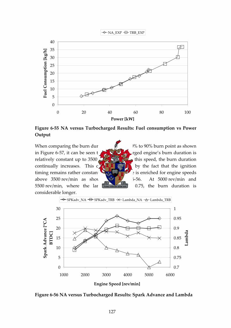
127
0
5
10
15
20
25
30
35
40
0 20 40 60 80 100
Power [kW]
FuelConsumption[kg/h]
NA_EXP TRB_EXP
Figure 6 55 NA versus Turbocharged Results: Fuel consumption vs Power
Output
When comparing the burn duration from the 10% to 90% burn point as shown
in Figure 6 57, it can be seen that the turbocharged engine’s burn duration is
relatively constant up to 3500 rev/min. Above this speed, the burn duration
continually increases. This can be explained by the fact that the ignition
timing remains rather constant, but the mixture is enriched for engine speeds
above 3500 rev/min as shown in Figure 6 56. At 5000 rev/min and
5500 rev/min, where the lambda is below 0.75, the burn duration is
considerable longer.
0
5
10
15
20
25
30
1000 2000 3000 4000 5000 6000
Engine Speed [rev/min]
SparkAdvance[°CA
BTDC]
0.7
0.75
0.8
0.85
0.9
0.95
1
Lambda
SPKadv_NA SPKadv_TRB Lambda_NA Lambda_TRB
Figure 6 56 NA versus Turbocharged Results: Spark Advance and Lambda

128
The reason why the burn duration at 4500 rev/min of the NA engine is longer
than that at 5000 rev/min is due to the timing that was retarded at
4500 rev/min. Thus the burn duration is not only dependent on the air/fuel
ratio, but also on the ignition timing.
20
21
22
23
24
25
26
27
28
29
30
1000 2000 3000 4000 5000 6000
Engine Speed [rev/min]
1090%BurnDuration[°CA]
NA_EXP TRB_EXP
Figure 6 57 NA versus Turbocharged Results: Burn Duration
Figure 6 58 compares the 50% burn point. This is the crank angle at which
50% of the mass of fuel was burned. It is an indication of ignition timing and
burn duration, however where ignition occurs before TDC, the 50% burn
point usually only occurs after TDC.
5
7
9
11
13
15
17
19
21
23
25
1000 2000 3000 4000 5000 6000
Engine Speed [rev/min]
50%BurnPoint[°CAATDC]
NA_EXP TRB_EXP
Figure 6 58 NA versus Turbocharged Results: 50% Burn Point
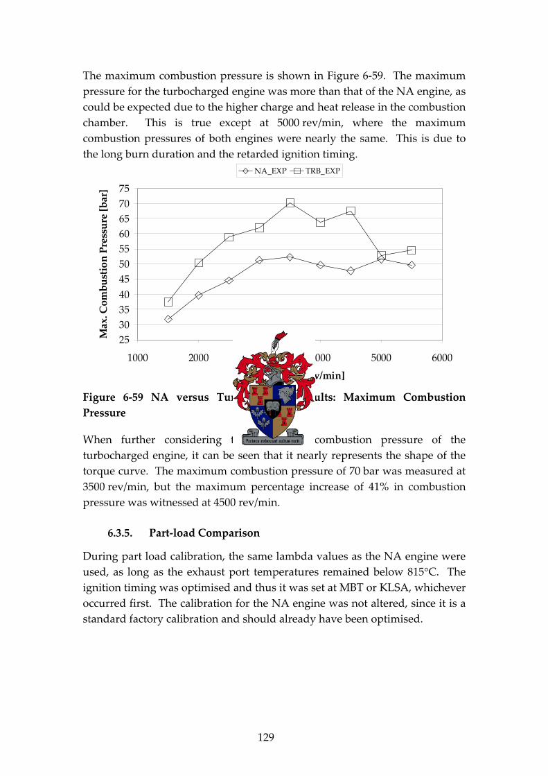
129
The maximum combustion pressure is shown in Figure 6 59. The maximum
pressure for the turbocharged engine was more than that of the NA engine, as
could be expected due to the higher charge and heat release in the combustion
chamber. This is true except at 5000 rev/min, where the maximum
combustion pressures of both engines were nearly the same. This is due to
the long burn duration and the retarded ignition timing.
25
30
35
40
45
50
55
60
65
70
75
1000 2000 3000 4000 5000 6000
Engine Speed [rev/min]
Max.CombustionPressure[bar]
NA_EXP TRB_EXP
Figure 6 59 NA versus Turbocharged Results: Maximum Combustion
Pressure
When further considering the maximum combustion pressure of the
turbocharged engine, it can be seen that it nearly represents the shape of the
torque curve. The maximum combustion pressure of 70 bar was measured at
3500 rev/min, but the maximum percentage increase of 41% in combustion
pressure was witnessed at 4500 rev/min.
6.3.5. Part load Comparison
During part load calibration, the same lambda values as the NA engine were
used, as long as the exhaust port temperatures remained below 815 C. The
ignition timing was optimised and thus it was set at MBT or KLSA, whichever
occurred first. The calibration for the NA engine was not altered, since it is a
standard factory calibration and should already have been optimised.

130
Testing was done only at two speeds, 2500 rev/min and 4000 rev/min, which
are the engine speeds where maximum torque was developed for the NA
engine and turbocharged engine, respectively. The maximum torque of the
NA engine at both speeds was used as the baseline, and assigned a value of
100%. All the comparisons are made in terms of percentage load, thus
percentage load of the NA engine at that speed.
Considering the part load SFC as presented in Figure 6 60, it is very
interesting to note that the SFC values for both engines at the different speeds
are fairly similar up to 60% load. At 80% load and 4000 rev/min, the
turbocharged engine’s exhaust temperature was very high and lambda was
reduced from 1.05 to 0.95 to keep the exhaust temperature within the limits,
thus the higher SFC for the turbocharged engine at 4000 rev/min can be
explained.
200
250
300
350
400
450
0 20 40 60 80 100 120 140 160Load [%]
SFC[g/KW.hr]
NA 4000 NA 2500 TRB 4000 TRB 2500
Figure 6 60 NA versus Turbocharged Results: Part load SFC
The main reason why the SFC at 100% load for the turbocharged engine is
better than the NA engine is due to the fact that the same lambda values
could not be reached due to the full load mixture enrichment necessary on the
NA engine. The turbocharged engine did not require a rich mixture to cool
the exhaust temperatures when operating at 100% of the NA engine’s torque.
Thus a lambda was adjusted for best fuel consumption while maintaining the
exhaust temperature below the upper limit. The spark advance and lambda
used during part load testing are presented in Figure 6 61 and Figure 6 62
respectively.

131
15
20
25
30
35
40
0 20 40 60 80 100 120 140 160Load [%]
SparkAdvance[°CABTDC]
NA_2500 TRB_2500 NA_4000 TRB_4000
Figure 6 61 NA versus Turbocharged Results: Part load Spark Advance
0.7
0.8
0.9
1
1.1
0 20 40 60 80 100 120 140 160Load [%]
Lambda
NA_2500 TRB_2500 NA_4000 TRB_4000
Figure 6 62 NA versus Turbocharged Results: Part load Lambda
At 4000 rev/min the turbocharged engine was severely limited by the high
exhaust temperatures and thus the lambda was reduced to keep the exhaust
temperature within the limits.

132
When operating the turbocharged engine at 2500 rev/min and lambda close to
1, about 92% of the fuel energy, as shown in Figure 6 63, can be accounted for
by the sum of shaft, cooling and exhaust energy, which is referred to as
Energy [%]. The exhaust energy is the potential thermal energy. The
chemical energy in the carbon monoxide (CO) and unburned fuel that exist in
the exhaust gas are not accounted for. For the NA engine about 88% of the
fuel energy can be accounted for when operating at lambda close to 1.
However, when lambda was decreased below 0.9, the percentage of
accounted energy decreased to 80% and decreased even further if lambda was
decreased more. This indicates that there is a lot of partially burned (carbon
monoxide) and unburned fuel leaving the engine through the exhaust. This is
verification of the fact that a large percentage of unaccounted, or “other”,
energy as shown in Figure 6 38 and Figure 6 39 is partially burned and
unburned fuel at WOT.
The reason why the NA engine can only account for about 88% of the fuel
energy when operating close to lambda 1, while the turbocharged engine can
account for about 92% of the fuel energy, is because the turbocharged engine
uses less fuel to develop the same amount of power. The actual amounts of
shaft, exhaust and cooling energy are very much similar for both engines, but
because the turbocharged engine uses less fuel it can account for a high
percentage of the fuel energy. The radiation losses for both engines should be
nearly the same because the operating temperatures of both engines were the
same. The unaccounted for energy can thus be attributed to unburned and
partially burned fuel in the exhaust as well as a percentage measurement
error.

133
0
20
40
60
80
100
0 20 40 60 80 100 120 140
Load [%]
Energy[%]
0.7
0.8
0.9
1
1.1
1.2
Lambda
NA_Energy TRB_Energy NA_Lambda TRB_Lambda
Figure 6 63 NA versus Turbocharged Results: Part load Energy Balance at
2500 rev/min
Probably the most significant results are represented by fuel flow and can be
seen in Figure 6 64. It can be seen that fuel flow at part load is nearly the
same for both engines. It is only at WOT that the turbocharged engine uses
more fuel than the NA engine. This extra fuel is not only used to cool the
exhaust temperature, but also to produce more power. This indicates that the
turbocharged engine not only develops more power, but could also match the
fuel economy at part load of its NA engine counterpart.
0
5
10
15
20
25
30
0 20 40 60 80 100 120 140 160
Load [%]
FuelFlow[kg/hr]
NA2500 TRB2500 NA4000 TRB4000
Figure 6 64 NA versus Turbocharged Results: Part load Fuel Flow

134
At a load equal to 100% of the NA WOT load the turbocharged engine is 7%
and 11% more fuel efficient at 2500 rev/min and 4000 rev/min respectively
and only 5% less fuel efficient at 80% and 4000 rev/min. It can thus be
concluded that a vehicle would be equally or more fuel efficient given the
same loading conditions.
When comparing part load fuel consumption, the turbocharged engine’s
consumption should be compared to a NA engine with the similar power
rating. Only then could the real advantage of having a small displacement,
high power output engine be put into perspective.
When comparing the rated power output of NA engines that are available on
the market at the time of writing this report, it was found that the 2 litre class
develops around 95 to 100 kW. Thus this turbocharged engine is 25% smaller
than similar rated NA engines. When comparing the peak torque the
turbocharged engine develops about 14% more torque than the average 2 liter
NA engine
Typical engine power requirements to maintain a constant speed on a level
road with a medium size passenger vehicle such as a mid ‘90s Toyota Corolla
was determined by Bell, A J (2005) and shown in Figure 6 65.
0
5
10
15
20
25
30
35
40 60 80 100 120 140
Road Speed [km/h]
RequiredEnginePower[kW]
Figure 6 65 Required Engine Power

135
To illustrate the advantage of a small turbocharged engine to a similar rated
bigger NA in this case a 1.6 liter turbocharged versus a 2.0 litre NA engine,
the torque of the 1.6 litre NA engine was scaled up by 25% which would be
the increase in displacement. It was assumed that the SFC of both NA
engines would be similar at a specific percentage load. These scaled torque
values were used as reference and maximum torque at a specific engine speed
was assigned a value of 100%. The torque developed by the turbocharged
engine was calculated as a percentage of the 2.0 liter NA engine’s torque. The
SFC was plotted against the turbocharged engine’s SFC as measured. This
was done for both 4000 rev/min and 2500 rev/min and is shown in Figure 6 66
and Figure 6 67 respectively. Superimposed on these graphs are the
percentage load required to maintain constant speeds of 80, 100 and 120 km/h
and corresponding SFC indicated by the shaded markers.
250
300
350
400
450
500
0 20 40 60 80 100 120Load [%]
SFC[g/KW.hr]
2.0L_4000 TRB_4000
80km/h
100km/h
120km/h
Figure 6 66 2.0L NA versus Turbocharged SFC at 4000 rev/min
The markers for 60km/h could not be included in either graph, since the
required power was outside the tested range.

136
200
250
300
350
400
450
0 20 40 60 80 100 120Load [%]
SFC[g/KW.hr]
2.0L_2500 TRB_2500
80km/h
100km/h
120km/h
Figure 6 67 2.0L NA versus Turbocharged SFC at 2500 rev/min
Table 6 1 illustrates the percentage fuel saved by using the turbocharged
engine instead of the big NA engine.
Table 6 1 Estimated Fuel Saving
Load [%] Engine Speed Road Speed [km/h] Fuel saving [%]
42 4000 120 5.3%
27 4000 100 9.6%
16 4000 80 12.8%
68 2500 120 1.0%
43 2500 100 8.8%
25 2500 80 11.6%
It can thus be concluded that the turbocharged engine is 12.8% and 11.6%
more fuel efficient than the bigger NA engine at 80km/h with engine speeds
of 4000 rev/min or 2500 rev/min respectively. The turbocharged engine is
more fuel efficient while having the capability to produce 14% and 8% more
torque than the bigger NA engine at 4000 rev/min and 2500 rev/min
respectively.

137
7. CONCLUSION
The development of a turbocharged spark ignition engine from a naturally
aspirated engine and the simulation and prediction of its performance were
the objectives and scope for this research project. These objectives were
successfully accomplished enabling the comparison of NA and turbocharged
engines.
Relevant literature was reviewed and was presented to the reader to
familiarise them with the theory behind turbocharging. The functionality of
the simulation package was briefly discussed. Simulation was used to
optimise valve timing and to illustrate the advantage that optimised valve
timing would have over the standard valve timing. Simulation was also used
to evaluate two exhaust manifold concepts. The exhaust manifold concept
evaluation showed that the concept using simple pulse converters was the
better of the two concepts. However, differences in overall performance were
very small and due to the advantage of simplicity and ease of manufacture
the concept without pulse converters was manufactured and used in actual
testing.
The engine was successfully converted to a turbocharged engine and testing
was completed successfully. The engine was then converted back to NA in
order to bracket the experiment and to ensure that neither the engine nor the
experimental apparatus has deviated during the evaluation. The engine
performed equally well before and after the converted period, thus the
engine’s condition remained consistent throughout the process while also
illustrating that the test facility produced reproducible results. This also
indicates the high degree of repeatability of the testing process.
The correlation between the measured and predicted torque for the NA
engine was within 6%. This error in predicting the NA engine torque can
mainly be attributed to the valve flow coefficients. The flow coefficients used
in the simulation were known to have not been accurately determined for this
specific engine. This inconsistency in the valve flow coefficients also caused a
shift in the predicted volumetric efficiency as a function of engine speed.
138
If the wastegate was controlled during simulation to match the boost pressure
that was measured on the actual engine, the predicted torque was within 9%
of the actual measured torque. It was found that the simulation predicted
more torque than was actually developed with the same boost pressure. The
trends of the predicted versus the measured engine parameters are the same,
as with the NA engine; therefore the simulation could be used to investigate
the sensitivity or influence of different design parameters on a desired output
such as torque.
The actual wastegate area and that predicted by the simulation did not
correlate well. The problem is believed to be due to inaccuracies both in the
simulated amount of air flowing through the wastegate and the calculation of
the wastegate area from the actual measured rack travel. The simulation
predicts very small opening areas when compared to what was calculated by
measuring the rack travel.
The turbocharged engine developed 96 kW at 5500 rev/min. At 2000 rev/min
84% of the maximum torque was produced, a maximum of 197 N m was
developed at 4000 rev/min and at 5500 rev/min 82% of the maximum torque
was still available. Thus the torque curve was not perfectly flat, but it was the
best that could be achieved without electronic boost control using the
standard cam shaft and valve timing. The turbocharged conversion increased
the maximum power by 37% and maximum torque by 48%.
When comparing this turbocharged engine with the NA engine, it has been
shown that this turbocharged engine could match the full load fuel economy
of the given NA engine up to the rated power of the NA engine, after which
the fuel consumption increased significantly as more power was developed.
This increase in fuel consumption was due to the rich mixture used to keep
the exhaust temperature below the limit.
The most significant fact was that at part load conditions this turbocharged
engine could match the SFC of the NA engine. Thus not only was more
power developed at WOT, but the fuel efficiency can be matched even at part
load. It is known that a big engine is less fuel efficient than a small engine
when both are developing the same torque at part load. Thus when
comparing the turbocharged engine to a average 2.0 litre NA engine of
similar rated maximum power output, the fuel savings of the turbocharged
engine at part load was estimated between 1% and 11.6% at 2500 rev/min and
between 5.3% and 12.8% at 4000 rev/min.
139
Developing a turbocharged engine from a NA engine is an attractive option
for motor companies that want to offer a higher performance engine in their
premium model, but do not have the resources to develop an all new engine.
It could also be used as a downsizing option and could be used to lower the
fleet average fuel consumption.
The first research question asked in the beginning was: what are the
implications of adding a turbocharger to a NA engine? The implications can
be summarised as:
It is possible to increase the maximum power output by 37% without
reducing the CR or increasing the engine speed at which it is
developed;
Using mechanical boost control and the NA engine’s camshaft and
valve timing, 82% of maximum torque was available from
2000 rev/min up to 5000 rev/min;
The loading on the components such as bearing forces would be
increased by the same percentage that the maximum torque is
increased provided the same speed range is considered;
The percentage increased loading on the cooling system is similar to
the percentage increase in maximum power output;
Part load efficiency could be matched if the turbocharged engine is
compared to a similar sized NA engine or the turbocharged engine
could be superior under certain conditions compared to an equally
powerful NA engine.
The second part of the research question: to determine whether the
performance of a turbocharged engine can be predicted accurately by using 1
D flow simulation? The simulation results can be summarised as:
The predicted torque was higher than the measured torque, but within
6% of the actual measured torque on the NA engine;
The predicted torque was higher than the measured torque, but within
9% of the actual measure torque on the turbocharged engine when
developing the same boost pressure;
The trends for both cases were very similar than that measured.
It can be concluded that if 6% and 9% accuracy on NA and turbocharged
engines respectively are within the acceptable limits of the purpose of the
simulations, then 1 D simulations would be accurate enough to be used.

140
8. RECOMMENDATIONS
When considering upgrading the performance of an engine by adding a
turbocharger, there are certain aspects that must be taken into consideration.
The strength of the crankshaft, connecting rods and pistons should be
investigated, since this will not only transfer more torque but also have higher
bearing loadings. The quality of the exhaust valve and seat are important due
to the higher exhaust temperatures typically experienced by a turbocharged
engine.
If a turbocharger with a water cooled bearing housing is used, the
degradation of the oil due to high temperatures in the turbocharger is not a
concern. The cooling system should, however, be upgraded depending on the
reserve capacity of the standard engine’s cooling system. As a general
guideline the cooling system should be able to cope with the same percentage
increase in loading as the percentage increase in power output.
It may be necessary to upgrade the fuel injectors to supply the extra fuel
needed to develop the higher power. If the fuel pressure is raised, the fuel rail
must be certified to be able to operate at this higher pressure. The fuel pump
must be able to deliver the desired flow rate at the designed operating
pressure and thus the fuel filter should also satisfy these requirements.
The exhaust system should be upgraded in order to keep the exhaust
backpressure (post turbine pressure) within reasonable limits due to the
higher airflow caused by the turbocharger. Since the turbine damps most of
the blow down noise that is carried by the exhaust gas, a free flow exhaust
system might be considered without increasing exhaust noise above the legal
limit. The amount of energy that the turbine can extract is proportional to the
pressure difference across the turbine, thus the lower the exhaust
backpressure the better. Care must be taken that, if the backpressure is too
low, it does not result in a situation where the wastegate is fully open, but the
boost pressure developed is too high. This could cause the turbine speed to
exceed its maximum and the results could be disastrous.

141
The variable wastegate actuator that was designed and manufactured proved
to be a useful and valuable tool. Although only one spring was used during
testing, different boost pressures could be achieved by only adjusting the
preload on the spring. If this variable wastegate actuator could be modified
such that it does not rely on the diaphragm to deform, its opening
characteristics would only be dependent on the spring and therefore it would
be a linear function of pressure and its operation would be consistent,
independent of the operating temperature.
Whilst not investigated specifically in this research, the importance of an
intercooler on a turbocharged engine cannot be over emphasised. The main
advantage of an intercooler is lower intake air temperatures. The lower air
temperatures will result in lower initial charge temperatures and would thus
reduce the chances that knock will occur. The lower air temperatures would
also make it possible to reduce the boost pressure, but still maintain the same
density of the air in the intake manifold. Lower boost pressure would further
reduce the chances that knock would occur. Thus, with reduced air
temperatures and reduced boost pressure, the ignition timing could be
advanced closer to MBT. Advancing the ignition timing may result in
reduced exhaust temperatures, which would enable leaner AFR mixtures
being used and thus improving fuel consumption. The use of lower boost
pressure might facilitate the use of a high CR which would greatly benefit
engine efficiency.
In this research project a turbocharged engine was developed, thus a test
engine is available in either NA or turbocharged format. This project sets the
pathway for further research and development in turbocharging. Possible
research could include valve optimisation coupled with boost pressure
optimisation, development of control strategies for electronic boost control
and electronic throttle control to minimise turbo lag.
Adding a turbocharger to a NA engine is not a simple or trivial task, but a
properly designed system will yield fruits in proportion with the engineering
excellence that was invested.

142
9. REFERENCES
Audi AG, 1998, Audi TT self study programme 207, Ingolstadt.
Azzoni, P, Moro, D, Ponti, F & Rizzoni, G, 1998, Engine and load torqueestimation with application to electronic throttle control, SAE paper, No. 980795,
Society of Automotive Engineers.
Bell, AJ, 2005, The effect of fuel formulation on the exhaust emissions of sparkignition engines, Ph.D. thesis, University of Stellenbosch.
Birmann, R, 1946, Exhaust energy converting means for internal combustionengines, US Patent, No. 2406656.
British Iron and Steel Research Association Metallurgy, 1953, Physicalconstants of some commercial steels at elevated temperatures, London Butterworth
Scientific Publications, London.
Ferguson, CR, 1986, Internal combustion engines – applied thermodynamics, JohnWiley, New York.
Gatowski, JA, Balles, EN, Chun, KM, Nelson, FE, Ekchian, JA, & Heywood,
JB, 1984, Heat release analysis of engine pressure data, SAE paper, No. 841359,
Society of Automotive Engineers.
Gerhardt, J, Honninger, H & Bischof, H, 1998, A new approach to functional andsoftware structure for engine management systems – BOSCH ME7, SAE paper, No
980801, Society of Automotive Engineers.
Heywood, JB, 1988, Internal combustion engine fundamentals, McGraw Hill,
United States of America.
Kingwill, AC, 2000, The calculation of the factors for power correction in IC engines,Internal report, Stellenbosch Automotive Engineering, October.
Kühnle, Kopp & Kausch, 1994, Öldurchsatz K0 mittlere Ölzufuhr, (datasheet).
Krabbendam, P, 2004, Telephonic interview, February, Stellenbosch.

143
Kröger, DG, 1998, Air cooled heat exchangers and cooling towers thermal flowperformance evaluation and design, Mechanical Engineering Department,
University of Stellenbosch.
Mabie, HH & Reinholtz, CF, 1987, Mechanisms and dynamics of machinery, 4th
edition, John Wiley, New York.
Mills, AF, 1995, Heat and mass transfer, Richard D. Irwin, United States of
America.
Moran, DP, Bell, AJ & Williams, PNT, 1997, RACER – Engine combustion dataacquisition and burn rate analysis system, Unpublished in house system
operations manual, Centre for Automotive Engineering, University of
Stellenbosch, September.
Nelder, JA & Mead, R, 1965, A simplex method for function minimization, TheComputer Journal Vol. 7, p. 308 313.
Press, WH, Teukolsky, SA, Vetterling, WT & Flannery, BP, 2001, Numericalrecipes in Fortran 77: The art of scientific computing, 2nd edition, Volume 1, The
Press Syndicate of the University of Cambridge, New York.
Ricardo, 2002, WAVE v5 Engine reference manual.
Sayers, AT, 1990, Hydraulic and compressible flow turbomachines, AT Sayers,
Cape Town.
Streib, H & Bischof, H, 1978, Electronic Throttle Control (ETC): A cost effectivesystem for improved emissions, fuel economy and driveability, SAE paper, No.
960338, Society of Automotive Engineers.
Van der Spuy, J, 2003, Personal interview, 2 October, Stellenbosch.
Van der Weshuizen, HJ, 2003, Computational and experimental investigation ofchamber design and combustion process interaction in a spark ignition engine, MSc.
thesis, University of Stellenbosch.
Venter, J, 1999, Automotive turbocharging, Car, December, p. 78.

144
Watson, N & Janota, M, 1971, Non steady flow in an exhaust system with a pulseconverter junction, Paper 27, Conference on Unsteady Flow, University of
Salford.
Watson, N & Janota, M, 1984, Turbocharging the internal combustion engine,MacMillan, Great Britain.

145
APPENDIX A OPTIMISATION ALGORITHMS
A.1. Nelder Mead Algorithm
The Nelder Mead algorithm (Nelder & Mead, 1965) was proposed as a
method for minimizing a real valued function F(x) for x n. Four scalar
parameters must be specified to define a complete Nelder Mead method:
coefficients of reflection ( ), expansion ( ), contraction ( ), and shrinkage ( ).
According to the original Nelder Mead paper, these parameters should
satisfy:
> 0; >1; > ; 0 < < 1; and 0 < < 1.(The relation > , while not stated explicitly in the original paper, is implicit
in the algorithm description and terminology.) The nearly universal choices
used in the standard Nelder Mead algorithm are:
= 1; = 2; = ½; and =½One iteration of the Nelder Mead algorithm for n variables:
1. Order: Order n+1 vertices to satisfy f(x1) f(x2) ….f(xn) f(xn+1)2. Reflect: Calculate the reflection point xr
))1( 1nr xxx (A 1)
wheren
i
i
n
xx
1 , Evaluate fr = f(xr)
if f1 fr fn, accept the reflected point xr and terminate iteration.
3. Expand: If fr < f1, calculate the expansion point xe,
1)1( ne xxx (A 2)
Evaluate fe = f(xe). If fe < f0, accept xe and terminate iteration; otherwise
(if fe fr), accept xr and terminate the iteration.
4. Contract: If fr fn, perform a contraction between x and the better of
xn+1 and xn.a. Outside: If fn fr fn+1, perform a outside contraction
1)1( nc xxx (A 3)
Evaluate fc = f(xc). If fc fr, accept xc and terminate the iteration; otherwise go
to step 5 (perform a shrink step).
b. Inside: If fr fn+1, perform a inside contraction
sncc xxx )1( (A 4)
Evaluate fcc = f(xcc). If fcc < fn+1, accept xcc and terminate the iteration; otherwise
go to step 5 (perform a shrink step).
5. Perform a shrink step: Evaluate f at the n points )( 11 xxxv ii ,

146
i = 2, …, n+1. The unordered vertices of the simplex at the next
iteration consist of x1, v2, …, vn+1.
A.2. Initial Value Scaling for Optimisation
Consider an optimisation problem with n variables and x1, x2, …, xn the initialvalues. Calculate a scaling factor Si by:
i
n
i ii xn
xS
.1 (A 5)
The scaled input is then calculated by:
i
ii Sx
y (A 6)
Then y1, y2, …, yn is used as the initial values. The boundary conditions must
also be scales accordingly. Thus when the optimisation has been completed,
the end values must be multiplied by the scaling factor to get the real value.

147
APPENDIX B TURBOCHARGER OIL FLOW
Figure B 1 K03 Oil Flow Specification (Kühnle, Kopp, Kausch, 1994)

148
APPENDIX C POWER CORRECTION FACTORS
For the purpose of determining the corrected power of internal combustion
engines, the following standard reference conditions are defined and
tabulated in Table C 1:
Table C 1 ECE Standard Reference Conditions
Quantity: Symbol: Reference Value: Unit:
Total barometric
pressurePr 100 kPa
Air temperature Tr 298 Kelvin [K]
Relative
humidityr 30 %
The ECE correction factor can be calculated as follows:
6.02.1 )298
273()
99( airin
a
T
PCF
Where:
)]3.237/()9.11678.16[(
)(
airinairinvsat
vsatbaroa
TTExpP
PPP
Note: Pa in kPa and Tairin in °C:
It must be stressed that the correction factor is only valid within a range of
±2% adjustment and must therefore be applied carefully.
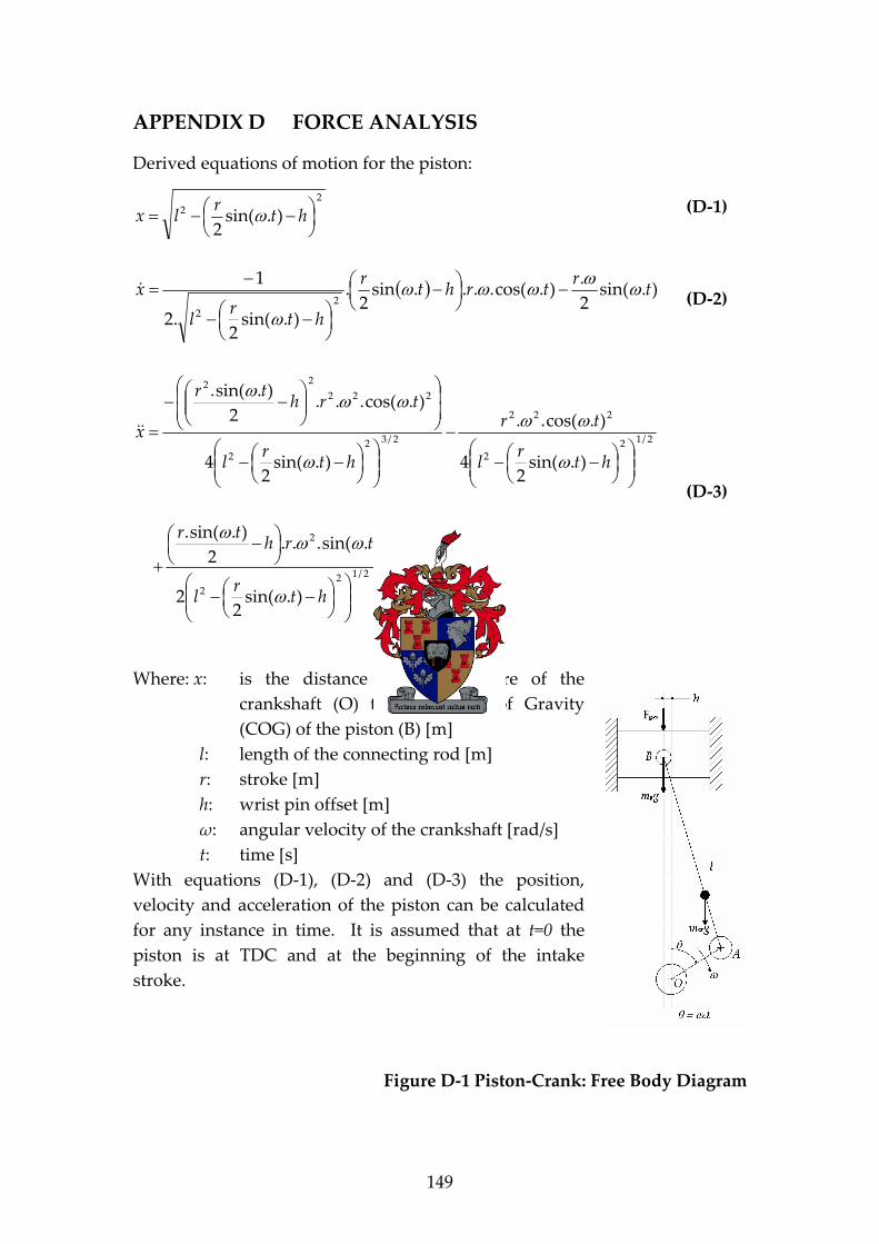
149
APPENDIX D FORCE ANALYSIS
Derived equations of motion for the piston:
22 ).sin(
2ht
rlx (D 1)
).sin(2
.).cos(....sin
2.
).sin(2
.2
12
2
tr
trhtr
htr
l
x(D 2)
2
).cos(..
).sin(2
2
).sin(...2
).sin(.
).sin(2
4
).cos(..
).sin(2
4
).cos(...2
).sin(.
2
2/122
2
2/122
222
2/322
222
22
tr
htr
l
trhtr
htr
l
tr
htr
l
trhtr
x
(D 3)
Where: x: is the distance from the centre of the
crankshaft (O) to the Centre of Gravity
(COG) of the piston (B) [m]
l: length of the connecting rod [m]
r: stroke [m]
h: wrist pin offset [m]
: angular velocity of the crankshaft [rad/s]
t: time [s]
With equations (D 1), (D 2) and (D 3) the position,
velocity and acceleration of the piston can be calculated
for any instance in time. It is assumed that at t=0 the
piston is at TDC and at the beginning of the intake
stroke.
Figure D 1 Piston Crank: Free Body Diagram