Application of the Transmissibility Concept in Transfer ... · Application of the T ransmissibility Concept in Transfer Path Analysis ... indirect way , ... In gene ral, all of these

Application of the Transmissibility Concept in Transfer Path Analysis

P. Gajdatsy1,2, K. Janssens1, Wim Desmet2, H. Van der Auweraer1 1LMS International NV Interleuvenlaan 68, 3001 Leuven, Belgium 2K. U. Leuven, Department of Mechanical Engineering Celestijnenlaan 300B, 3001 Leuven, Belgium email: [email protected]

Abstract In recent years, there has been a renewed interest in developing faster and simpler transfer path analysis (TPA) methods. A dominant class of these new approaches, often referred to as Operational Path Analyses (OPA), is designed to achieve this goal by using only operational data in conjunction with the application of the transmissibility concept. Despite the reduction in measurement time and complexity, these suffer from a number of limitations, such as problems related to the estimation of transmissibility, or the unreliability of the results due to cross coupling between path inputs, etc, which makes them prone to errors. Some of these only apply to one specific method while others are common to all transmissibility based approaches. The goal of this paper is to identify and describe these limitations and point out the potential dangers of applying such methods without taking these into account.

1 Introduction

The concept of transmissibility has been around for many years [1-3], but has recently gained new interest, especially in the field of structural health monitoring and operational modal analysis [4]. Furthermore, it has also found its way into other areas, such as noise path analysis. The link between some new ad-hoc approaches to noise path analysis and the transmissibility concept was demonstrated in [5]. The motivation for the research into new noise path analysis techniques is that the classical Transfer Path Analysis (TPA) method, despite having become a well-established and reliable technique for tackling NVH problems, still remains a time consuming and complex procedure. The use of transmissibilities apparently offers a possibility for a significant reduction in measurement time and complexity. Among these new TPA methods, two groups can be distinguished. Earlier publications [6, 7] describe an approach which corresponds to the use of transmissibilities to replace the frequency response functions (FRFs) to describe the transfer paths [5, 8]. As opposed to this, a recently published method [9] uses them in an indirect way, for the in-situ estimation of the frequency response functions of the system, thus eliminating the need for experimental FRF measurements. In general, all of these methods are referred to as Operational Transfer Path Analysis (OTPA), or simply Operational Path Analysis (OPA) methods, since just the operational data in itself is sufficient for the analysis. But a fundamental question arises, namely, as to what extent the notions of “Transfer Paths” and “Transfer Path Analysis” are still applicable to the results obtained this way. The goal of this paper is to give an answer to this question by identifying the limitations pertaining to both types of approaches. In order to achieve this, first a general system model is introduced which is then followed by an overview of the basic ideas of the transmissibility concept. Then the transmissibility based OTPA methods are discussed in detail and finally, the identified limitations are analyzed through both analytical considerations and numerical simulations. Partial results of this study have already been published at various conferences [10-13].

Appears in MSSP vol. 24(7) - ISMA2010 special issue 3909

2 Transfer Path Analysis (TPA)

2.1 Basic TPA formulation

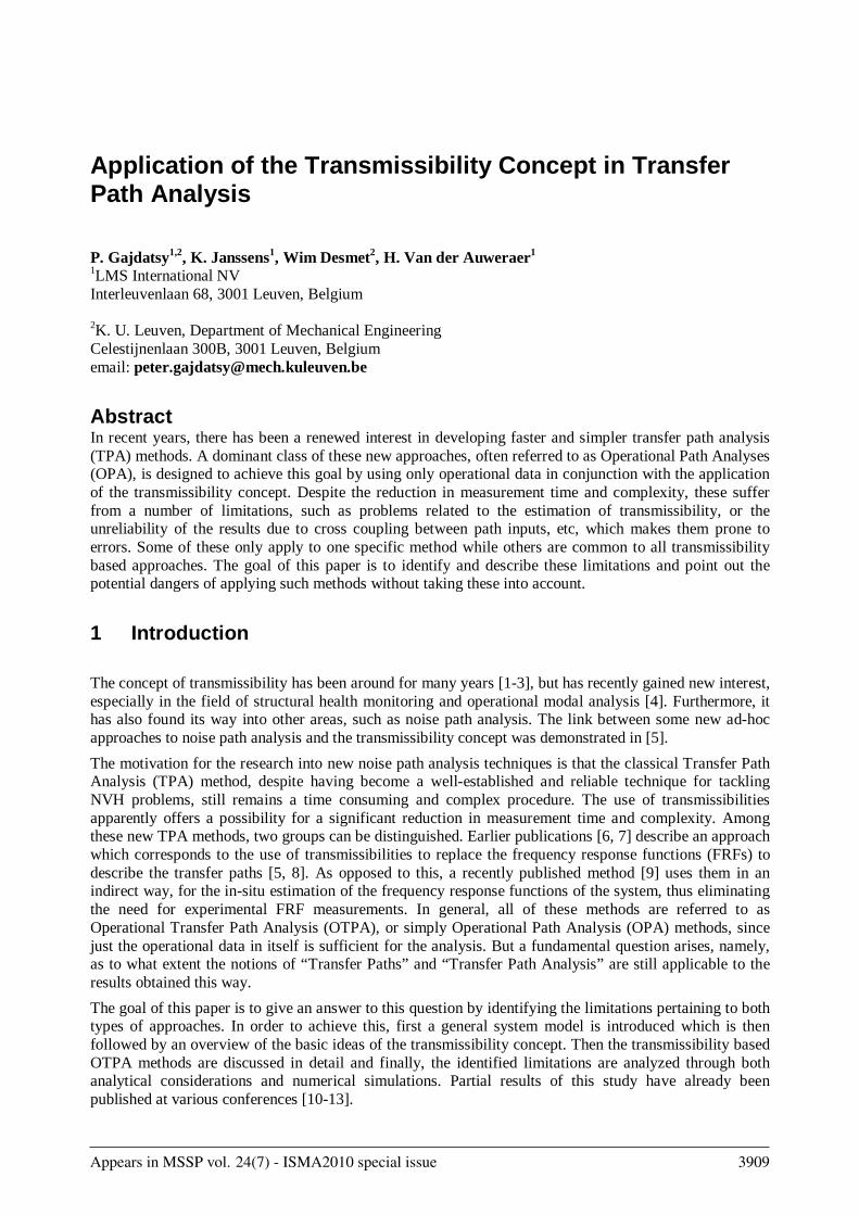
The transfer path model used throughout the following discussions is the classical source-path-receiver TPA model which dates back to the '80s [14-16]. It is first briefly reviewed and the key ideas and its limitations are discussed. The basic assumption of this TPA model is that the global system can be divided into an active and a passive part, the former containing the sources, the latter the transmission paths and receiver points. A schematic representation is shown in Fig. 1. At the interface between the two parts, structural or acoustic loads can be defined depending on the type of coupling. These excitations are then propagated to the receiver points through the transfer paths. Generally, the loads are force (Fi) or volume velocity (Qj), e.g. an engine mount or the air intake orifice respectively, and the receiver responses are sound pressure (ptarget) or acceleration (e.g. the sound at the driver’s ear or steering wheel vibration). The transfer paths are represented by their corresponding Frequency Response Functions (FRF), which are often called Noise Transfer Functions (NTF’s). Each of them describes the relationship between one input degree-of-freedom (DoF) and one response DoF. There is also a second group of FRF’s in the model, denoted by Hij in Fig. 1 and usually referred to as “local FRF’s”. These FRF’s express the relationship between the responses at the input DoF’s (apn, ppi) and also at additional response locations, which are called overdetermination points (apk). This model presumes a causal load-response relationship and that all the FRF’s are system characteristics of the global system.

Figure 1: General TPA model

Based on these considerations, the response at the receiver location pt can therefore be expressed as:

)(Q.)(NTF)(F.)(NTF)(p j

r

1jji

n

1iit

(1)

where Fi (i = 1…n) denotes the interface forces due to structural loads, Qj (j = 1…r) the volume velocities due to acoustic loads, and NTFi and NTFj the corresponding noise transfer functions.

Active Subsystem

Fn

Hij ap1

NTFj

ppi

pt

Qj

…

Passive Subsystem

apk

… ap2

F1 F2

apn

3910 PROCEEDINGS OF ISMA2010 INCLUDING USD2010

Further, a passive side response api can be written as

j

ijjpi HFa (2)

where, Hij represents the corresponding local FRF’s. All of these quantities depend on the dynamics of the actual system. Therefore, if the system is modified and its dynamic behavior is changed then these input quantities have to be identified again. An alternative solution would be to directly characterize the excitation source of the system [29], but this is beyond the scope of classical TPA. Frequently, the contributions from structural loads or the contributions from acoustic loads are separately investigated. The former case is generally referred to as “Transfer Path Analysis”, while the latter as “Acoustic Source Quantification” or also as “Panel Contribution Analysis” in case the acoustic sources are radiating panels [17-18]. The underlying general principles however remain the same. For the sake of simplicity, the discussions in the following chapters will be restricted to a single case in which the inputs are structural loads and the target is a single pressure response.

2.2 Practical limitations of classical TPA

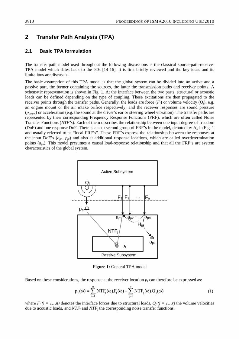
TPA is a powerful methodology to assess dominant noise source contributions. The most common way to visualize the results of a TPA analysis is the so called partial path contribution (PPC) plot, such as the one shown in Fig.2. In such a plot each row shows the partial contribution of a single path – which is the load multiplied by its corresponding NTF – to the target response as a function of RPM for a given engine order. However, such plot should be handled with care as it only displays the magnitude information but not the phase relationship between the different paths. For example, the black rectangle shows a region where transfer paths 3 and 4 seem to have a high contribution yet the total contribution remains low. This is due to a canceling phase relationship between the transfer paths, compensating each other. The phase information therefore should always be taken into account during an analysis. To facilitate this, the results are often also plotted on Bode or vector diagrams.

RPM

Pat

hs

1000 2000 3000 4000 5000 6000

1

2

3

4

5

6

Sum55

60

65

70

75

dB

Figure 2: A partial path contribution (PPC) plot

The test procedure to build a conventional TPA model typically requires two basic steps, first the identification of the operational loads during in-operation tests (e.g. run-up, run-down, etc.) e.g. on the road or on a chassis dyno; and secondly the estimation of the NTF’s from experimental tests (e.g. hammer impact test, shaker test, etc.). The procedure is similar for both structural and acoustical loading cases, but the practical implementation is governed by the nature of the signals and loads.

TRANSFER PATH ANALYSIS AND SOURCE IDENTIFICATION 3911

As for the second step, a number of reliable and well-known methods exist to measure and estimate both acoustic and structural NTF’s. For example, reciprocity techniques are commonly used, exciting at the acoustic response location and measuring corresponding accelerations at the load location [19]. However, with regard to the estimation of the operational loads, they remain the main factor in the accuracy of the analysis [20-23]. Presently, there are three classical measurement methods in use. The most straightforward approach is to measure the forces directly by using dedicated measuring devices such as e.g. load cells for structural forces. But such direct measurements are not feasible in the majority of the cases because load cells require space and well-defined support surfaces. This either distorts the original mounting conditions or simply makes mounting impossible. The second, and most widely used, approach is the mount stiffness method which can be used in cases when the active and passive system components are connected through flexible mounts. This approach calculates the transmitted force from the relative operational displacement across a given mount and the corresponding known mount stiffness profile.

2piai

ii

))(a)(a().(K)(F

(3)

Fi is the force in the mount, Ki is the mount stiffness profile and aai and api are the active and passive side mount accelerations. The mount stiffness method is a fast method, but its main drawback is that accurate mount stiffness data are seldom available and as most mounts are non-linear, they depend on the load conditions (pre-loads) and excitation amplitudes. The third approach is the inverse force identification method which estimates the operational forces from a large set of (mostly local) operational indicator accelerations and the corresponding FRF matrix. For a set of n operational forces Fnx1, m operational acceleration indicator responses, amx1, are measured on the passive side, along with the corresponding FRF matrix Hmxn between all inputs and all indicator responses. The operational forces then can be estimated by multiplying amx1 with the pseudo-inverse of Hmxn:

})({a.)]([H })({F (4)

This equation is calculated separately for each frequency. The number of indicator responses (m) must exceed the number of forces (n), typically by a factor 2 as a rule of thumb, in order to minimize ill-conditioning problems during the pseudo-inverse calculation. The main drawback of this approach is the need to perform a large number of FRF measurements to build the full Hmxn matrix, which is time consuming. Moreover, the active part has to be removed for the FRF measurements, further increasing the duration of the measurement [21-22]. Despite these limitations this method is used most often in the NVH field, and therefore in this article it is referred to as the classical TPA approach. For the sake of completeness, it must be mentioned that there are some other approaches, such as combining numerical models with measurement data [24], the use of a different approach to FRF measurement [25] or the use of Fast TPA approaches for assessing global subsystem responses [5,8], but these are not yet as widespread as the classical methods described previously.

3 Transmissibility

The common feature in most of the recently proposed, so-called operational TPA methods is that they attempt to avoid the time consuming stage of FRF measurements by relying on the in-operation measurement of system transmissibilities. Transmissibility expresses the relationship between two responses in a system. Let apa and apb denote these two responses, Fi the single force acting on the system and Hai, Hbi the corresponding transfer functions from Hij. The transmissibility can be formulated then, as:

)(H)(H

)(F)(H)(F)(H

)(a)(a

Tbi

ai

ibi

iai

pb

paab

(5)


Basically, transmissibility is the ratio of two FRF’s in a single input case. Naturally, this formulation can also be extended to MIMO systems [1-4]. In order to gain more insight into the meaning of the previous result, the transfer functions are rewritten in a pole-zero form in Eq. (6), as it was formulated by Guillaume et al in [3]. Here D() represents the denominator polynomial whose roots are the system poles and Nxx() the numerator polynomial containing the zeros of the transfer function. An important fact is that while Nxx() is specific to each transfer function, D() is common to every member of Hij. Therefore the transmissibility reduces to Eq. (7).

)(D)(N)(Hand

)(D)(N)(H bi

biai

ai

(6)

)(N)(NT

bi

aiab

(7)

This result has a number of important consequences. First of all it can be seen that the peaks in the magnitude of the transmissibility functions do not coincide with the peaks in the FRF’s since the poles of one transfer function become the zeros of the transmissibility Tab. Another important observation is that the transmissibility depends on the location of the forces [3]. In case an additional force is acting on the system the transmissibilities will change since the corresponding FRF’s will be changed. One way to acquire the transmissibility functions of a system is to measure them experimentally before the structure is placed in operation, which is the common practice in structural health monitoring applications. However, in other cases, such as OMA and OPA, they need to be estimated from operational data.

4 Operational Transfer Path Analyses

In order to overcome the test-time limitations of the traditional TPA approach and to speed up the analysis process, a number of solutions and improvements have been proposed as mentioned in Section 1, making different trade-offs regarding speed, accuracy, detail of analysis and causality [5-8]. During the following discussions the classical TPA approach is used as a reference, in spite of its shortcomings. The reasons for this choice are twofold: firstly because it is the most well-known approach in the NVH field and secondly because the new methods in general claim to be equivalent to it. In some of these methods the transmissibility concept is directly applied to the TPA model, by replacing the transfer functions with transmissibilities. The goal of these methods is to use only operational data to derive ‘TPA-like’ results without the need for all the additional measurements characteristic of classical TPA approaches. This is achieved by using a different TPA-like model in which the target response is formulated using operational responses measured at the load locations instead of the loads themselves. Since the mathematical formulation is similar to that of TPA, there is often confusion about the terminology, which unfortunately leads to an incorrect use of the method and interpretation of the results. These methods are discussed in Section 4.1. Another type of transmissibility based TPA approach, described in Section 4.2, uses the concept in an indirect way. The system description remains the classical source-path-receiver TPA model, but the transfer functions are estimated from the transmissibilities [9, 26]. Although this avoids most of the pitfalls of the previous group it still has some limitations.

4.1 OPA methods based on direct application of transmissibility

The approaches belonging to this group are referred to as “OPA” or “OPA method”. The basic idea of the OPA method was described in [6] as an ad-hoc measurement method and was then further elaborated by


[7], however, without linking this approach to the underlying transmissibility formulation. In [5], this approach was shown to be an implicit application of MIMO transmissibility theory. Using the notation of Fig. 1 the mathematical model for a pressure target can be expressed as:

)(p.)(T)(a.)(T)(p pj

r

1jjpi

n

1iit

(8)

where api (i = 1…n) are the body side mount accelerations representing the structural paths, pj (j = 1…r) operational pressures representing the acoustic sources and, finally, Ti and Tj the transmissibilities between the acceleration and pressure inputs at the load locations and the target response. For the sake of clarity the () term, denoting the frequency dependence, is omitted in the following. The transmissibilities can be estimated from the operational input and response data using an H1 estimator:

'}p,a{}p,a{T}'p,a{p}p,a{.TppTa.Tp ppppppppt

r

1jpjjpi

n

1iit

(9)

1-aata

-1

ppppppt SS'}p,a{}p,a{}'p,a{pT (10)

The sign denotes the complex conjugate transpose of the vectors, the horizontal line the average, the <…> sign a row vector, the {…} a column vector, […] a matrix, and taS and aaS stand for the averaged cross- and autopower matrix respectively. At first sight this approach looks promising since there is no need for time consuming FRF measurements. All that is required is some operational data and the results can be immediately calculated. Despite the fact that this approach claims to be similar to the classical TPA approach, there are a number of fundamental differences: first of all, the OPA model is not causal, as opposed to the classical TPA model. Instead of a load-response relationship, it is based on a response-response relationship, which means that while in TPA one can draw a conclusion as to what effect a certain load has on the total response, in OPA one can only talk, with a few exceptions, about a similarity, or in other words, a "co-existence" relationship between the target and the input responses. Secondly, the transmissibilities are not system characteristics but depend on the position and number of forces acting on the system, as it was mentioned in Section 3, and thirdly, transmissibilities are not equivalent to the NTF’s. However, there might be some situations where such a method can still be useful for troubleshooting. Earlier studies [10-13] showed that the necessary conditions for this are i) the forces acting on the structure should have a low correlation with each other in order to have good transmissibility and path contribution estimates, ii) cross coupling between paths should be small, meaning that the effect of a given force must be the most prominent in the corresponding input response and negligible in all other input responses and iii) all paths must be taken into account. All these limitations are thoroughly elaborated through a set of examples in Section 5.

4.2 OPA method based on indirect application of transmissibility

Despite the fact that this recently published method [9] also calls itself an OPA approach, it is fundamentally different from the previous one. In this method the transmissibilities are used indirectly, only to estimate the NTF’s, but not to replace them and the classical TPA model is preserved. This approach avoids most of the problems related to the direct transmissibility methods and the results can actually be interpreted in the same way as in the traditional TPA. Still it has a few limitations on its own. The most obvious one is that the method requires a large number of incoherent forces acting on the active part and a number of known forces acting at the connection points during operation. This requirement limits the applicability of the method since in most practical situations only a few, and even then often coherent sources are present on the active part (e.g. engine imbalance), and as for the known forces on the


passive part, it is usually quite complicated, if not impossible, to excite the connection points during operation, let alone at the exact same DOF as the operational forces.

5 Limitations of the direct OPA methods

In the following, the required conditions for the OPA method, mentioned in Section 4.1, are discussed:

low coherence between input forces

low cross coupling between input responses

all active paths included in the analysis These conditions need to be fulfilled to obtain physically meaningful results through the direct OPA methods. In order to assess their effect from a practical point of view, a measurement based test case is used. An extensive dataset is synthesized from an existing and well-validated experimental TPA model originating from an engine noise TPA dataset of a 4-cylider car in run-up conditions (from 1000 to 6000 rpm). It contains 21 structural paths: 3 engine mounts and 4 subframe mounts measured in three orthogonal directions, plus 1 pressure target at the driver’s location. A high quality analysis was performed and the model was validated for consistency. The use of such “representative” dataset is preferred over both pure simulation data, which can not include all real-life critical factors, and over pure experimental data, which is hard to control to allow consistent comparisons. The resulting dataset includes: i) operational mount forces F21x1 for orders 0.5 up to 10, ii) body FRF matrix H21x21 and iii) NTF21x1 between forces and pressure target. Based on this data, a number of numerical simulations are carried out to re-synthesize the load and response data, such as the operational passive-, sometimes called body side accelerations and pressure responses, for the separate assessment of each condition. The results are shown in PPC plots. The analysis only treats structural transfer paths. A related investigation regarding acoustic sources is discussed in [28]. Traditionally the similarity between synthesized and measured target pressure is used as an indication of the quality of the synthesis. In the case of classical TPA this is a valid approach, but when it comes to OPA this has to be discarded and the individual path contributions must be compared. This is due to the fact that the considered OPA methods could be called “backward-forward” calculations. The target signal is used already during the estimation of the transmissibilities, as seen in Eq. 11, therefore it is not surprising that the path contributions sum up to the measured target in most cases. In the following steps the error on the individual path contributions is used to indicate the quality and reliability of the direct OPA method.

5.1 Low coherence for good transmissibility estimates

The first critical element of the OPA method is the ill-conditioning problem related to estimating transmissibilities from operational data. As described in Section 4.1 they are typically estimated by using an H1 estimator, well-known from classical Least-Squares (LS) estimation:

-1aata SS}T{ (11)

The basic condition for performing this operation is the invertibility of the averaged autopower matrix aaS which is equal to having a full rank matrix. This requires that in the build-up or averaging of the power spectra, a number of different conditions at least equal to the number of paths are realized at each frequency. This might be obtained by combining tests under different conditions. For example, during an engine run-up, each frequency will, with increasing RPM, be excited by different orders, each of these causing a different phase relation between the engine mount responses. Averaging over the RPM range or in different driving conditions with varying torques also decorrelates the autopower matrix. In most


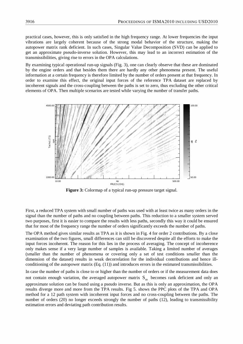
practical cases, however, this is only satisfied in the high frequency range. At lower frequencies the input vibrations are largely coherent because of the strong modal behavior of the structure, making the autopower matrix rank deficient. In such cases, Singular Value Decomposition (SVD) can be applied to get an approximate pseudo-inverse solution. However, this may lead to an incorrect estimation of the transmissibilities, giving rise to errors in the OPA calculations. By examining typical operational run-up signals (Fig. 3), one can clearly observe that these are dominated by the engine orders and that besides them there are hardly any other phenomena present. The useful information at a certain frequency is therefore limited by the number of orders present at that frequency. In order to examine this effect, the original input forces of the reference TPA dataset are replaced by incoherent signals and the cross-coupling between the paths is set to zero, thus excluding the other critical elements of OPA. Then multiple scenarios are tested while varying the number of transfer paths.

10.00 500.00HzFRLE:S (CH1)

1000.00

4500.00

rpm

Tach

o1 (T

1)

50.00

100.00

dB Pa

Figure 3: Colormap of a typical run-up pressure target signal.

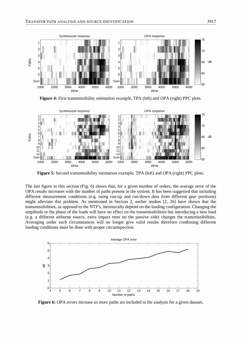
First, a reduced TPA system with small number of paths was used with at least twice as many orders in the signal than the number of paths and no coupling between paths. This reduction to a smaller system served two purposes, first it is easier to compare the results with less paths, secondly this way it could be ensured that for most of the frequency range the number of orders significantly exceeds the number of paths. The OPA method gives similar results as TPA as it is shown in Fig. 4 for order 2 contributions. By a close examination of the two figures, small differences can still be discovered despite all the efforts to make the input forces incoherent. The reason for this lies in the process of averaging. The concept of incoherence only makes sense if a very large number of samples is available. Taking a limited number of averages (smaller than the number of phenomena or covering only a set of test conditions smaller than the dimension of the dataset) results in weak decorrelation for the individual contributions and hence ill-conditioning of the autopower matrix (Eq. (11)) and introduces errors in the estimated transmissibilities. In case the number of paths is close to or higher than the number of orders or if the measurement data does not contain enough variation, the averaged autopower matrix aaS becomes rank deficient and only an approximate solution can be found using a pseudo inverse. But as this is only an approximation, the OPA results diverge more and more from the TPA results. Fig 5. shows the PPC plots of the TPA and OPA method for a 12 path system with incoherent input forces and no cross-coupling between the paths. The number of orders (20) no longer exceeds strongly the number of paths (12), leading to transmissibility estimation errors and deviating path contribution results.


RPM

OPA response

1000 2000 3000 4000 5000 6000

1

2

3

4

5

6

Sum

RPM

Synthesized response

Pat

hs

1000 2000 3000 4000 5000 6000

1

2

3

4

5

6

Sum55

60

65

70

75

dB

Figure 4: First transmissibility estimation example, TPA (left) and OPA (right) PPC plots.

RPM

OPA response

1000 2000 3000 4000 5000 6000

1 2 3 4 5 6 7 8 9101112

Sum

RPM


Pat

hs

1000 2000 3000 4000 5000 6000

1 2 3 4 5 6 7 8 9101112

Sum 55

60

65

70

75

dB

Figure 5: Second transmissibility estimation example, TPA (left) and OPA (right) PPC plots.

The last figure in this section (Fig. 6) shows that, for a given number of orders, the average error of the OPA results increases with the number of paths present in the system. It has been suggested that including different measurement conditions (e.g. using run-up and run-down data from different gear positions) might alleviate this problem. As mentioned in Section 2, earlier studies [2, 26] have shown that the transmissibilities, as opposed to the NTF's, intrinsically depend on the loading configuration. Changing the amplitude or the phase of the loads will have no effect on the transmissibilities but introducing a new load (e.g. a different airborne source, extra impact tests on the passive side) changes the transmissibilities. Averaging under such circumstances will no longer give valid results therefore combining different loading conditions must be done with proper circumspection.

4 5 6 7 8 9 10 11 12 13 14 15 16 17 18 190

1

2

3

4

5

6

dB

Number of paths

Average OPA error

Figure 6: OPA errors increase as more paths are included in the analysis for a given dataset.


So far, an ideal situation has been presented in which all the input forces are incoherent. However, in a real test case, the forces are always partially correlated due to the modal behavior of the system, which means that to a significant extent they carry the same information, thus reducing the rank of the autopower matrix and increasing the error of the estimation. Therefore, in such a real-life application with correlated inputs, the average error can be expected to be much higher than the ideal example shown here.

5.2 Cross-coupling between the path inputs

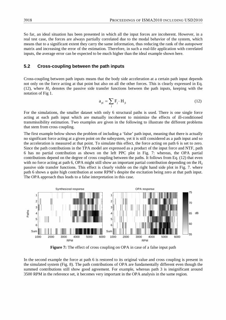
Cross-coupling between path inputs means that the body side acceleration at a certain path input depends not only on the force acting at that point but also on all the other forces. This is clearly expressed in Eq. (12), where Hij denotes the passive side transfer functions between the path inputs, keeping with the notation of Fig 1.

j

jijpi HFa (12)

For the simulations, the smaller dataset with only 6 structural paths is used. There is one single force acting at each path input which are mutually incoherent to minimize the effects of ill-conditioned transmissibility estimation. Two examples are given in the following to illustrate the different problems that stem from cross coupling. The first example below shows the problem of including a ‘false’ path input, meaning that there is actually no significant force acting at a given point on the subsystem, yet it is still considered as a path input and so the acceleration is measured at that point. To simulate this effect, the force acting on path 6 is set to zero. Since the path contributions in the TPA model are expressed as a product of the input force and NTF, path 6 has no partial contribution as shown on the left PPC plot in Fig. 7: whereas, the OPA partial contributions depend on the degree of cross coupling between the paths. It follows from Eq. (12) that even with no force acting at path 6, OPA might still show an important partial contribution depending on the Hij passive side transfer functions. This effect is clearly visible on the right hand side plot in Fig. 7. where path 6 shows a quite high contribution at some RPM’s despite the excitation being zero at that path input. The OPA approach thus leads to a false interpretation in this case.

RPM

OPA response

1000 2000 3000 4000 5000 6000

1

2

3

4

5

6

Sum

RPM


Pat

hs

1000 2000 3000 4000 5000 6000

1

2

3

4

5

6

Sum55

60

65

70

75

dB

Figure 7: The effect of cross coupling on OPA in case of a false input path

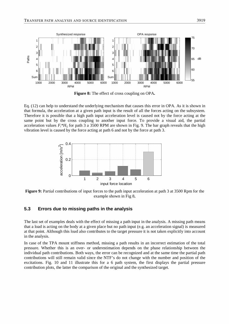
In the second example the force at path 6 is restored to its original value and cross coupling is present in the simulated system (Fig. 8). The path contributions of OPA are fundamentally different even though the summed contributions still show good agreement. For example, whereas path 3 is insignificant around 3500 RPM in the reference set, it becomes very important in the OPA analysis in the same region.


RPM

OPA response

1000 2000 3000 4000 5000 6000

1

2

3

4

5

6

Sum

RPM


Pat

hs

1000 2000 3000 4000 5000 6000

1

2

3

4

5

6

Sum55

60

65

70

75

dB

Figure 8: The effect of cross coupling on OPA.

Eq. (12) can help to understand the underlying mechanism that causes this error in OPA. As it is shown in that formula, the acceleration at a given path input is the result of all the forces acting on the subsystem. Therefore it is possible that a high path input acceleration level is caused not by the force acting at the same point but by the cross coupling to another input force. To provide a visual aid, the partial acceleration values Fi*Hij for path 3 a 3500 RPM are shown in Fig. 9. The bar graph reveals that the high vibration level is caused by the force acting at path 6 and not by the force at path 3.

1 2 3 4 5 60

0.2

0.4

input force location

acce

lera

tion

[m/s

2 ]

Figure 9: Partial contributions of input forces to the path input acceleration at path 3 at 3500 Rpm for the

example shown in Fig 8.

5.3 Errors due to missing paths in the analysis

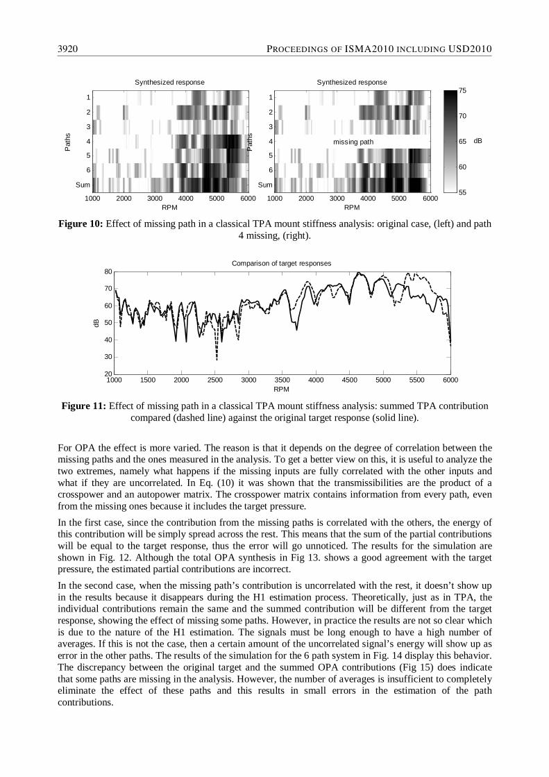
The last set of examples deals with the effect of missing a path input in the analysis. A missing path means that a load is acting on the body at a given place but no path input (e.g. an acceleration signal) is measured at that point. Although this load also contributes to the target pressure it is not taken explicitly into account in the analysis. In case of the TPA mount stiffness method, missing a path results in an incorrect estimation of the total pressure. Whether this is an over- or underestimation depends on the phase relationship between the individual path contributions. Both ways, the error can be recognized and at the same time the partial path contributions will still remain valid since the NTF’s do not change with the number and position of the excitations. Fig. 10 and 11 illustrate this for a 6 path system, the first displays the partial pressure contribution plots, the latter the comparison of the original and the synthesized target.


RPM


Pat

hs

1000 2000 3000 4000 5000 6000

1

2

3

4

5

6

Sum

RPM


Pat

hs

1000 2000 3000 4000 5000 6000

1

2

3

4

5

6

Sum55

60

65

70

75

dBmissing path

Figure 10: Effect of missing path in a classical TPA mount stiffness analysis: original case, (left) and path

4 missing, (right).

1000 1500 2000 2500 3000 3500 4000 4500 5000 5500 600020

30

40

50

60

70

80

dB

RPM

Comparison of target responses

Figure 11: Effect of missing path in a classical TPA mount stiffness analysis: summed TPA contribution

compared (dashed line) against the original target response (solid line).

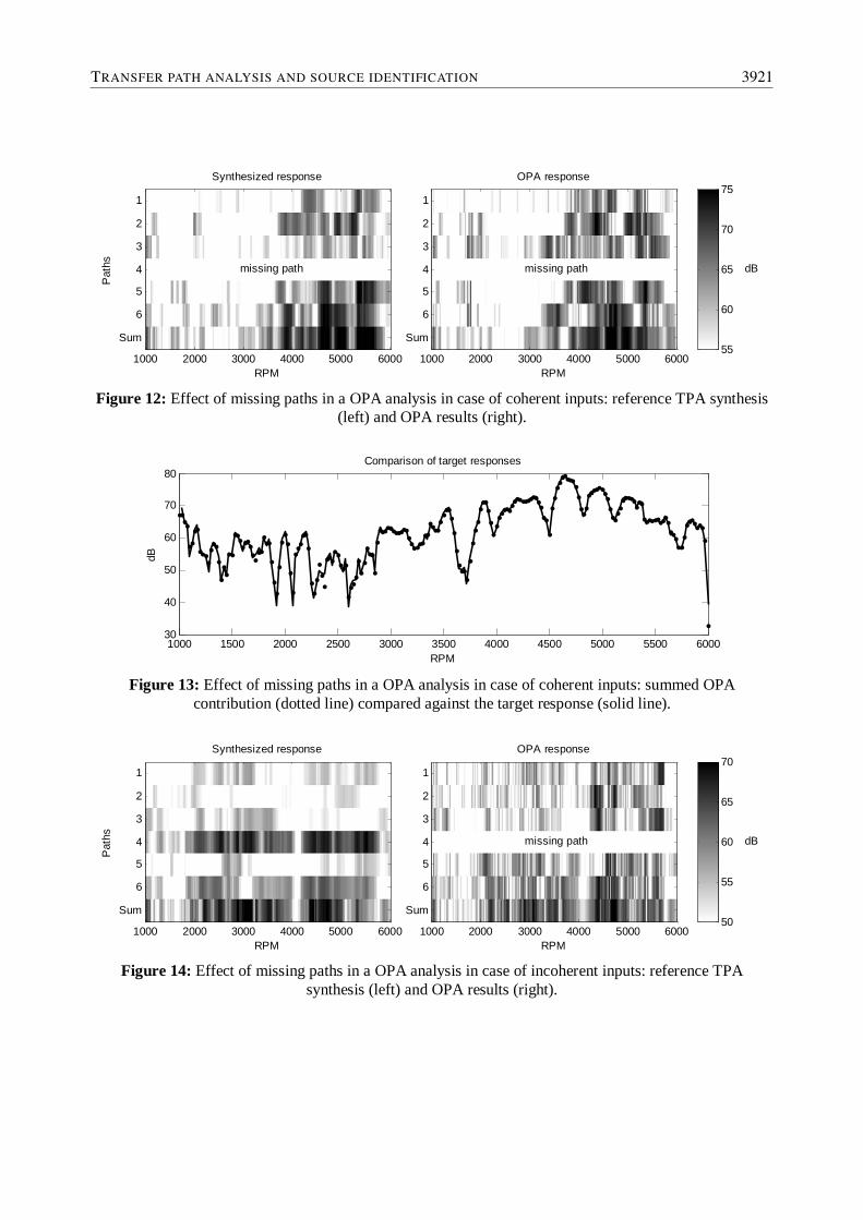
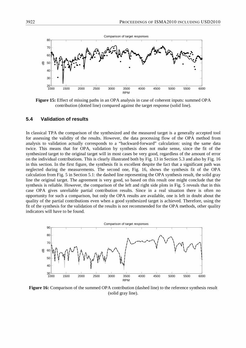
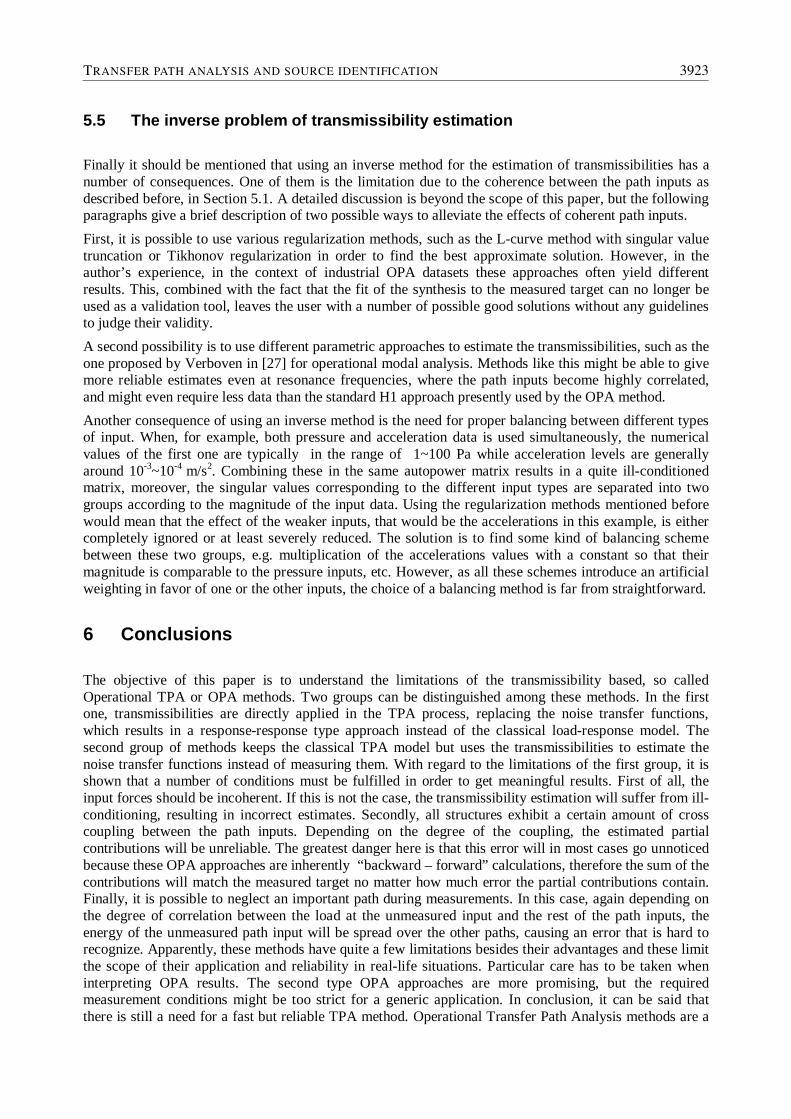
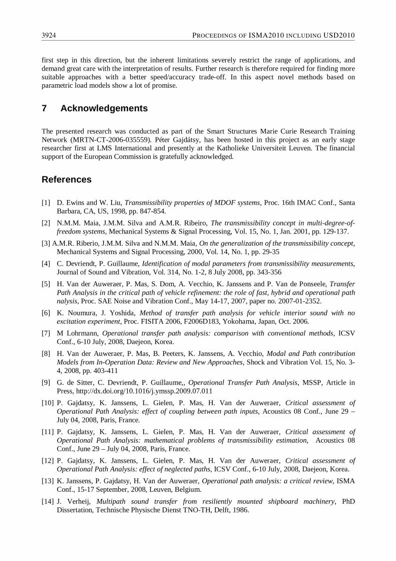
For OPA the effect is more varied. The reason is that it depends on the degree of correlation between the missing paths and the ones measured in the analysis. To get a better view on this, it is useful to analyze the two extremes, namely what happens if the missing inputs are fully correlated with the other inputs and what if they are uncorrelated. In Eq. (10) it was shown that the transmissibilities are the product of a crosspower and an autopower matrix. The crosspower matrix contains information from every path, even from the missing ones because it includes the target pressure. In the first case, since the contribution from the missing paths is correlated with the others, the energy of this contribution will be simply spread across the rest. This means that the sum of the partial contributions will be equal to the target response, thus the error will go unnoticed. The results for the simulation are shown in Fig. 12. Although the total OPA synthesis in Fig 13. shows a good agreement with the target pressure, the estimated partial contributions are incorrect. In the second case, when the missing path’s contribution is uncorrelated with the rest, it doesn’t show up in the results because it disappears during the H1 estimation process. Theoretically, just as in TPA, the individual contributions remain the same and the summed contribution will be different from the target response, showing the effect of missing some paths. However, in practice the results are not so clear which is due to the nature of the H1 estimation. The signals must be long enough to have a high number of averages. If this is not the case, then a certain amount of the uncorrelated signal’s energy will show up as error in the other paths. The results of the simulation for the 6 path system in Fig. 14 display this behavior. The discrepancy between the original target and the summed OPA contributions (Fig 15) does indicate that some paths are missing in the analysis. However, the number of averages is insufficient to completely eliminate the effect of these paths and this results in small errors in the estimation of the path contributions.


RPM


Pat

hs

1000 2000 3000 4000 5000 6000

1

2

3

4

5

6

Sum

RPM

OPA response

1000 2000 3000 4000 5000 6000

1

2

3

4

5

6

Sum55

60

65

70

75

dBmissing pathmissing path

Figure 12: Effect of missing paths in a OPA analysis in case of coherent inputs: reference TPA synthesis

(left) and OPA results (right).

1000 1500 2000 2500 3000 3500 4000 4500 5000 5500 600030

40

50

60

70

80

dB

RPM


Figure 13: Effect of missing paths in a OPA analysis in case of coherent inputs: summed OPA

contribution (dotted line) compared against the target response (solid line).

RPM


Pat

hs

1000 2000 3000 4000 5000 6000

1

2

3

4

5

6

Sum

RPM

OPA response

1000 2000 3000 4000 5000 6000

1

2

3

4

5

6

Sum50

55

60

65

70

dBmissing path

Figure 14: Effect of missing paths in a OPA analysis in case of incoherent inputs: reference TPA

synthesis (left) and OPA results (right).


1000 1500 2000 2500 3000 3500 4000 4500 5000 5500 600020

30

40

50

60

70

80dB

RPM


Figure 15: Effect of missing paths in an OPA analysis in case of coherent inputs: summed OPA

contribution (dotted line) compared against the target response (solid line).

5.4 Validation of results

In classical TPA the comparison of the synthesized and the measured target is a generally accepted tool for assessing the validity of the results. However, the data processing flow of the OPA method from analysis to validation actually corresponds to a “backward-forward” calculation: using the same data twice. This means that for OPA, validation by synthesis does not make sense, since the fit of the synthesized target to the original target will in most cases be very good, regardless of the amount of error on the individual contributions. This is clearly illustrated both by Fig. 13 in Section 5.3 and also by Fig. 16 in this section. In the first figure, the synthesis fit is excellent despite the fact that a significant path was neglected during the measurements. The second one, Fig. 16, shows the synthesis fit of the OPA calculation from Fig. 5 in Section 5.1: the dashed line representing the OPA synthesis result, the solid gray line the original target. The agreement is very good, so based on this result one might conclude that the synthesis is reliable. However, the comparison of the left and right side plots in Fig. 5 reveals that in this case OPA gives unreliable partial contribution results. Since in a real situation there is often no opportunity for such a comparison, but only the OPA results are available, one is left in doubt about the quality of the partial contributions even when a good synthesized target is achieved. Therefore, using the fit of the synthesis for the validation of the results is not recommended for the OPA methods, other quality indicators will have to be found.

1000 1500 2000 2500 3000 3500 4000 4500 5000 5500 600030

40

50

60

70

80

90

dB

RPM


Figure 16: Comparison of the summed OPA contribution (dashed line) to the reference synthesis result

(solid gray line).


5.5 The inverse problem of transmissibility estimation

Finally it should be mentioned that using an inverse method for the estimation of transmissibilities has a number of consequences. One of them is the limitation due to the coherence between the path inputs as described before, in Section 5.1. A detailed discussion is beyond the scope of this paper, but the following paragraphs give a brief description of two possible ways to alleviate the effects of coherent path inputs. First, it is possible to use various regularization methods, such as the L-curve method with singular value truncation or Tikhonov regularization in order to find the best approximate solution. However, in the author’s experience, in the context of industrial OPA datasets these approaches often yield different results. This, combined with the fact that the fit of the synthesis to the measured target can no longer be used as a validation tool, leaves the user with a number of possible good solutions without any guidelines to judge their validity. A second possibility is to use different parametric approaches to estimate the transmissibilities, such as the one proposed by Verboven in [27] for operational modal analysis. Methods like this might be able to give more reliable estimates even at resonance frequencies, where the path inputs become highly correlated, and might even require less data than the standard H1 approach presently used by the OPA method. Another consequence of using an inverse method is the need for proper balancing between different types of input. When, for example, both pressure and acceleration data is used simultaneously, the numerical values of the first one are typically in the range of 1~100 Pa while acceleration levels are generally around 10-3~10-4 m/s2. Combining these in the same autopower matrix results in a quite ill-conditioned matrix, moreover, the singular values corresponding to the different input types are separated into two groups according to the magnitude of the input data. Using the regularization methods mentioned before would mean that the effect of the weaker inputs, that would be the accelerations in this example, is either completely ignored or at least severely reduced. The solution is to find some kind of balancing scheme between these two groups, e.g. multiplication of the accelerations values with a constant so that their magnitude is comparable to the pressure inputs, etc. However, as all these schemes introduce an artificial weighting in favor of one or the other inputs, the choice of a balancing method is far from straightforward.

6 Conclusions

The objective of this paper is to understand the limitations of the transmissibility based, so called Operational TPA or OPA methods. Two groups can be distinguished among these methods. In the first one, transmissibilities are directly applied in the TPA process, replacing the noise transfer functions, which results in a response-response type approach instead of the classical load-response model. The second group of methods keeps the classical TPA model but uses the transmissibilities to estimate the noise transfer functions instead of measuring them. With regard to the limitations of the first group, it is shown that a number of conditions must be fulfilled in order to get meaningful results. First of all, the input forces should be incoherent. If this is not the case, the transmissibility estimation will suffer from ill-conditioning, resulting in incorrect estimates. Secondly, all structures exhibit a certain amount of cross coupling between the path inputs. Depending on the degree of the coupling, the estimated partial contributions will be unreliable. The greatest danger here is that this error will in most cases go unnoticed because these OPA approaches are inherently “backward – forward” calculations, therefore the sum of the contributions will match the measured target no matter how much error the partial contributions contain. Finally, it is possible to neglect an important path during measurements. In this case, again depending on the degree of correlation between the load at the unmeasured input and the rest of the path inputs, the energy of the unmeasured path input will be spread over the other paths, causing an error that is hard to recognize. Apparently, these methods have quite a few limitations besides their advantages and these limit the scope of their application and reliability in real-life situations. Particular care has to be taken when interpreting OPA results. The second type OPA approaches are more promising, but the required measurement conditions might be too strict for a generic application. In conclusion, it can be said that there is still a need for a fast but reliable TPA method. Operational Transfer Path Analysis methods are a


first step in this direction, but the inherent limitations severely restrict the range of applications, and demand great care with the interpretation of results. Further research is therefore required for finding more suitable approaches with a better speed/accuracy trade-off. In this aspect novel methods based on parametric load models show a lot of promise.

7 Acknowledgements

The presented research was conducted as part of the Smart Structures Marie Curie Research Training Network (MRTN-CT-2006-035559). Péter Gajdátsy, has been hosted in this project as an early stage researcher first at LMS International and presently at the Katholieke Universiteit Leuven. The financial support of the European Commission is gratefully acknowledged.

References

[1] D. Ewins and W. Liu, Transmissibility properties of MDOF systems, Proc. 16th IMAC Conf., Santa Barbara, CA, US, 1998, pp. 847-854.

[2] N.M.M. Maia, J.M.M. Silva and A.M.R. Ribeiro, The transmissibility concept in multi-degree-of-freedom systems, Mechanical Systems & Signal Processing, Vol. 15, No. 1, Jan. 2001, pp. 129-137.

[3] A.M.R. Riberio, J.M.M. Silva and N.M.M. Maia, On the generalization of the transmissibility concept, Mechanical Systems and Signal Processing, 2000, Vol. 14, No. 1, pp. 29-35

[4] C. Devriendt, P. Guillaume, Identification of modal parameters from transmissibility measurements, Journal of Sound and Vibration, Vol. 314, No. 1-2, 8 July 2008, pp. 343-356

[5] H. Van der Auweraer, P. Mas, S. Dom, A. Vecchio, K. Janssens and P. Van de Ponseele, Transfer Path Analysis in the critical path of vehicle refinement: the role of fast, hybrid and operational path nalysis, Proc. SAE Noise and Vibration Conf., May 14-17, 2007, paper no. 2007-01-2352.

[6] K. Noumura, J. Yoshida, Method of transfer path analysis for vehicle interior sound with no excitation experiment, Proc. FISITA 2006, F2006D183, Yokohama, Japan, Oct. 2006.

[7] M Lohrmann, Operational transfer path analysis: comparison with conventional methods, ICSV Conf., 6-10 July, 2008, Daejeon, Korea.

[8] H. Van der Auweraer, P. Mas, B. Peeters, K. Janssens, A. Vecchio, Modal and Path contribution Models from In-Operation Data: Review and New Approaches, Shock and Vibration Vol. 15, No. 3-4, 2008, pp. 403-411

[9] G. de Sitter, C. Devriendt, P. Guillaume,, Operational Transfer Path Analysis, MSSP, Article in Press, http://dx.doi.org/10.1016/j.ymssp.2009.07.011

[10] P. Gajdatsy, K. Janssens, L. Gielen, P. Mas, H. Van der Auweraer, Critical assessment of Operational Path Analysis: effect of coupling between path inputs, Acoustics 08 Conf., June 29 – July 04, 2008, Paris, France.

[11] P. Gajdatsy, K. Janssens, L. Gielen, P. Mas, H. Van der Auweraer, Critical assessment of Operational Path Analysis: mathematical problems of transmissibility estimation, Acoustics 08 Conf., June 29 – July 04, 2008, Paris, France.

[12] P. Gajdatsy, K. Janssens, L. Gielen, P. Mas, H. Van der Auweraer, Critical assessment of Operational Path Analysis: effect of neglected paths, ICSV Conf., 6-10 July, 2008, Daejeon, Korea.

[13] K. Janssens, P. Gajdatsy, H. Van der Auweraer, Operational path analysis: a critical review, ISMA Conf., 15-17 September, 2008, Leuven, Belgium.

[14] J. Verheij, Multipath sound transfer from resiliently mounted shipboard machinery, PhD Dissertation, Technische Physische Dienst TNO-TH, Delft, 1986.


[15] J. Verheij, Experimental procedures for quantifying sound paths to the interior of road vehicles, Proc. 2nd Int. Conf. on Vehicle Comfort, Bologna, Italy, Oct.14-16, 1992, pp. 483-491.

[16] F.X. Magrans, Method of measuring transmission paths, J. Sound Vib., Vol 73, No. 3, pp. 321-330 (1981)

[17] J. Verheij, Hoebrichts, Thompson, Acoustical source strength characterisation for heavy road vehicles engines in connection with pass-by noise, 3rd ICSV Conf., June 1994, Montreal (CND).

[18] P. van der Linden, J. Schnur, T. Schomburg, Quantifying the noise emission of engine oilsumps, valve covers, etc. using artificial excitation, 5th ICSV Conf., Adelaide (AU), December 1997.

[19] P. van der Linden, J. Fun, Using mechanical-acoustic reciprocity for diagnosis of structure borne sound in vehicles, SAE Noise & Vibration Conference & Exposition, May 1993, Traverse City, MI, USA, SAE paper no. 93130.

[20] J. Starkey and G. Merril, On the ill-conditioned nature of indirect force measurement techniques, Int. J. Analyt. Exp. Modal Anal., Vol. 4, No. 3, 1989, pp. 103-108.

[21] P. van der Linden and H. Floetke, Comparing inverse force identification and the mount stiffness force identification methods for noise contribution analysis, Proc. 2004 ISMA Conf., Leuven, Belgium, Sept. 2004.

[22] P. Mas, P. Sas and K. Wyckaert, Indirect force identification based upon impedance matrix inversion: a study on statistical and deterministical accuracy, Proc. 1994 ISMA Conf., Leuven, Belgium, Sept. 12-14, 1994.

[23] M. Blau, Indirect measurement of multiple excitation force spectra by FRF matrix inversion: influence of errors in statistical estimates of FRFs and response spectra, Acta Acustica united with Acustica, Volume 85, Number 4, July/August 1999 , pp. 464-479 (16)

[24] P. van der Linden, F. Gerard, K. Michiels, H. Van der Auweraer, D. Storer, Body in white panel noise assessment through spatial and modal contribution analysis, Proc. ISMA-25, Leuven, Belgium, Sept. 2000, pp.1361-1368.

[25] W. Biermayer, F. Brandl, R. Hoeldrich, A. Sontacchi, S. Brandl, H. H. Priebsch, Efficient Transfer Path Analysis for Vehicle Sound Engineering, JSAE 2008 Annual Congress, 21-23 May, 2008, Pacifico Yokohama, Japan

[26] P. Guillaume, C. Devriendt, G. De Sitter, An operational modal analysis approach based on parametrically identified multivariable transmissibilities, MSSP, Article in Press, http://dx.doi.org/10.1016/j.ymssp.2009.02.015

[27] P. Verboven, Frequency domain system identification for modal analysis. PhD Thesis, Department of Mechanical Engineering, Vrije Universiteit Brussel, Belgium, avrg.vub.ac.be, 2002.

[28] D. Tcherniak, A.P. Schuhmacher, Application of Transmissibility Matrix Method to NVH Source Contribution Analysis, IMAC XVII, 9-12 February 2009, Orlando, Florida, USA

[29] D. de Klerk and D.J. Rixen, Component transfer path analysis method with compensation for test bench dynamics, Mechanical Systems and Signal Processing, 2010 (in press, available online), doi:10.1016/j.ymssp.2010.01.006



Documents

Application of the Transmissibility Concept in Transfer ... · Application of the T ransmissibility Concept in Transfer Path Analysis ... indirect way , ... In gene ral, all of these