Engineering Structures 141 (2017) 175–183

Contents lists available at ScienceDirect

Engineering Structures

journal homepage: www.elsevier .com/ locate /engstruct

Cosine based and extended transmissibility damage indicatorsfor structural damage detection

http://dx.doi.org/10.1016/j.engstruct.2017.03.0300141-0296/� 2017 Elsevier Ltd. All rights reserved.

⇑ Corresponding author at: Division of Computational Mechanics, Ton Duc ThangUniversity, Ho Chi Minh City, Viet Nam.

E-mail addresses: magd.abdelwahab@tdt.edu.vn, magd.abdelwahab@ugent.be(M. Abdel Wahab).

Yun-Lai Zhou a, Magd Abdel Wahab b,c,d,⇑aDepartment of Civil and Environmental Engineering, National University of Singapore, 2 Engineering Drive 2, Singapore 117576, SingaporebDivision of Computational Mechanics, Ton Duc Thang University, Ho Chi Minh City, Viet Namc Faculty of Civil Engineering, Ton Duc Thang University, Ho Chi Minh City, Viet Namd Soete Laboratory, Faculty of Engineering and Architecture, Ghent University, Technologiepark, Technologiepark Zwijnaarde 903, B-9052 Zwijnaarde, Belgium

a r t i c l e i n f o a b s t r a c t

Article history:Received 15 November 2016Revised 12 February 2017Accepted 16 March 2017Available online 24 March 2017

Keywords:Structural damage detectionTransmissibilityModal assurance criterionCosine similarity measure

Structural damage detection using vibration-based techniques and transmissibility is investigated andproposed with elaborating the mathematical interrelationship between modal assurance criterion(MAC) and cosine similarity measure. From this interrelationship, two new damage indicators, namelycosine based indicator (CI) and extended transmissibility damage indicator (ETDI), are drawn out. EvenMAC and cosine similarity measure are normally adopted separately; their kernel agrees well with eachother. In this study, we extend these two indicators, derive two new damage indicators, CI and ETDC, andapply them in a transmissibility based structural damage detection technique. In order to verify the fea-sibility of the developed damage indicators, experimental data for a three-story benchmark structure isadopted. The results from the benchmark demonstrate well performance of both indicators in damagedetection, which might imply their potential applicability in further real engineering structures.

� 2017 Elsevier Ltd. All rights reserved.

1. Introduction

Structural health monitoring (SHM) has undergone boomingadvancement during the last decades with numerous techniquesraised and applied in real engineering projects in both time andfrequency domain, empirically based and model methods. Forvibration-based techniques, the reader may refer to [1,2], wherein [1], vibration-based approaches were summarized and in [2],the survey mainly illustrated the vibration-based techniques incomposite structures. Note that this survey also followed the struc-tural damage identification philosophy that damage detectioncould be considered as a statistical pattern recognition paradigm,which summarized SHM into a four step paradigm: (1) OperationalEvaluation; (2) Data Acquisition, Fusion, and Cleansing; (3) FeatureExtraction and Information Condensation and (4) Statistical ModeDevelopment for Feature Discrimination. For more details aboutthis paradigm, the reader may refer to [1].

SHM development can be summarized into two main parts: a)testing and measuring techniques and b) methodologies for themeasured data interpretation. As to the testing and measuring

techniques, along with the history, SHM underwent various tech-niques such as oil penetrating, modal testing, acoustic emission,ultrasonic testing, eddy current and magnetic particle testing. Onthe other hand, methodologies like probabilistic based, patternrecognition based, and so on, are also developed to interpret themeasured data such as strain based and impedance based. Evenmore options exist nowadays for SHM, vibration based techniques[3–7] still hold an essential role since its easy conduction but effec-tive and efficient in SHM in both civil engineering and mechanicalengineering.

Modal testing and modal analysis serve as the fundamental invibration-based techniques, which also underwent two mainphases: a) experimental modal analysis (EMA) and b) operationalmodal analysis (OMA). EMA frequently makes use of laboratorytesting of specimens to extract modal parameters, such as naturalfrequencies, mode shapes and Frequency Response Functions(FRFs) in order to avoid the operating conditions. The drawbacksof this method are obvious as it might be convenient for smallspecimens, while for heavy, large structures such as wind turbines,dam and so on, it will be definitely challenging, or in some casesimpossible. Another shortcoming is the cost that the laboratorytesting needs to transfer the specimen from operating conditioninto prototype. This cost includes the reinstallation, dismantling,transferring, testing, which will impose more expenses and doesnot make the method a cost-effective approach. The OMA tries to

176 Y.-L. Zhou, M. Abdel Wahab / Engineering Structures 141 (2017) 175–183

avoid these drawbacks by directly testing and analyze the mea-sured responses. Generally speaking, statistical based methods willbe taken into consideration for this kind of analysis since theunknown loads shall restrict the analysis to be responses based.

Among all output-based techniques, transmissibility, one con-cept raised several decades ago, has served as an essential featurein system identification, damage identification, i.e. detection, local-ization, and quantification. For details about transmissibility, thereader may refer to [8–12]. The transmissibility was elaboratedin theoretical advancement perspective in [8,9] by addressing theforce transmissibility, direct transmissibility and certain applica-tions. The study in [10] focused on the damage detection historicaldevelopment with transmissibility by generally summarizing thekey investigations during last decades. In [11], transmissibilitywas reviewed in a general perspective from both theoretical pro-cess and engineering applications, while in [12], a concept of trans-missibility selection was presented in order to reduce thecomputation expenses, but simultaneously maintaining the capac-ity of detecting damage effectively with elaborating the historicaldevelopment of transmissibility theory and application in a con-densed view. In addition to the development of transmissibilitytheory, vibration based SHM techniques are summarized intotwo categories, namely physical model and data/statistical model.The physical model based techniques require the physical model asprior in order to have a better analysis with Finite Element Analysis(FEA), while the data model based techniques try to identify dam-ages according to the structural responses under operating/testingcondition.

Modal assurance criterion (MAC), firstly raised in late 1970s[13,14], has served as one essential indicator in the later damagedetection history. MAC, initially designed for correlation analysis[13–16], has been widely applied to discriminate the damage fea-tures from baseline [12,17–25]. The key idea is to construct a dam-age sensitive feature and to use data analysis tools, to developdamage indicators using MAC [12,17–26] or artificial neural net-works (ANNs) [27] to discriminate the current structural patternfrom the baseline. On the one hand, different indicators were con-structed, such as Frequency Domain Assurance Criterion (FDAC) toanalyze the correlation between the analytically calculated and theexperimentally measured FRF [15]. This indicator, FDAC, laterextended to a particular form known as Response Vector AssuranceCriterion (RVAC) intending to measure the correlation betweenoperational deflection shapes [16]. Several years later, by averagingRVAC, Detection and Relative Damage Quantification Indicator(DRQ) was built to detect and quantify the damage relatively[17,19]. Henceforth, DRQ was extended to transmissibility baseddamage detection and quantification [23]. In [28], the frequencyband selection was pointed out that the noise-contaminated bandshould be avoided in order to reduce the influence in final results.In [21], MAC was applied to the vector of inverse delta transmissi-bilities for identifying the damage. Similar application also waspresented in [22] for transmissibility coherence, compressed trans-missibility [12], transmissibility based distance measure [24]. In[25], coordinate modal assurance criterion (COMAC) was utilizedto detect damage for a helicopter composite main rotor blade. Inaddition, MAC was also applied to build objective function inmulti-objective framework based damage localization and quan-tification [18,20], where analytical and experimental flexibilitieswere taken into consideration.

With regard to cosine similarity measure, which was raised dec-ades ago, it was defined as the inner product of two vectors dividedby the product of their lengths [29], expressing the angle betweenthese two vectors. Cosine similarity measure has been applied invarious engineering applications [30–35], such as in pattern recog-nition [30], image recognition [32], neutrosophic sets medicaldiagnosis [33] and damage identification [31,34,35]. In [31], cosine

similarity measure was taken for comparison with other distancemeasures like Euclidean distance, Manhattan distance, L-infinity,Mahalanobis distance in K-nearest neighbor (KNN) classificationmethod and was applied to Z-24 bridge data sets as case study.This study revealed that similarity measures have significantimpact on the pattern recognition success rate. Furthermore, inRefs [34,35] cosine similarity measure was applied to the transmis-sibility compressed by principal component analysis (PCA) in dam-age recognition, where it showed well performance in identifyingthe damages.

Even though MAC and cosine similarity measure have been sep-arately utilized in the past, it might be beneficial for researchers topoint out the inter-connection between them. This study aims tounveil the inter-connection between MAC and cosine similaritymeasure, and thus to propose a comparison between them andsome previously developed indicators for transmissibility baseddamage detection methodology. The remaining sections of thepaper are summarized as follows. Section 2 gives the fundamentalsof transmissibility, MAC and cosine similaritymeasure. In Section 3,the damage detection paradigm using transmissibility is presented.Section 4 utilizes experimental data of three-story benchmarkstructure as case study. Finally concluding remarks are summa-rized in Section 5.

2. Theoretical fundamentals

2.1. Transmissibility fundamentals

Transmissibility serves as an essential feature for damagedetection [8–12,23,26,36,37] as it does not require the measure-ment of forces, and thus leading to a wide application, and integra-tion with other methods. Transmissibility, generally, is defined asthe ratio between two dynamic outputs, and for a linearmultiple-degree-of-freedom (MDOF) system subjected to a har-monic loading at a given position, it will be expressed as:

Tði;jÞðxÞ ¼ XiðxÞXjðxÞ ð1Þ

where Xi and Xj are the complex amplitudes of the systemresponses, xi(t) and xj(t), respectively, and x is the frequency. In thisstudy, Fourier transform is adopted in obtaining the response spec-trum. Certainly Laplace transform can also be adopted, the finaldetected results will be the same.

Transmissibility can be estimated by several approaches, forinstance, directly using the two outputs. In addition, one can alsouse FRFs if available, or taking average by using auto- and spectra:

Tði;jÞðxÞ ¼ XiðxÞXjðxÞ ¼

XiðxÞ � XiðxÞXjðxÞ � XiðxÞ ¼

Gði;iÞðxÞGðj;iÞðxÞ ð2Þ

where G means the auto- or cross-spectrum. Note that by analogof coherence estimation in FRFs, transmissibility coherence (TC)can be drawn out. For details, the reader may refer to [11,22],where TC is systematically discussed and applied in damagedetection and quantification, especially for small nonlinearityquantification. Herein in this study, transmissibility is derivedby Eq. (2).

2.2. Modal assurance criterion (MAC)

MAC is normally defined with some vectors, like FRFs, transmis-sibility and so on. For a general case, e.g. two vectors (two col-umns), A and B, it can be expressed as:

MACðA;BÞ ¼ ðATBÞ2

ðATAÞðBTBÞ ð3Þ

1

Y.-L. Zhou, M. Abdel Wahab / Engineering Structures 141 (2017) 175–183 177

where MAC 2[0,1], ()T means the transpose. Note that this will bethe same in all equations discussed hereinafter. Furthermore, whenMAC equals to ‘0’, it means no correlation between A and B, whilewhen MAC equals to ‘1’, it means the highest correlation betweenA and B takes place [25].

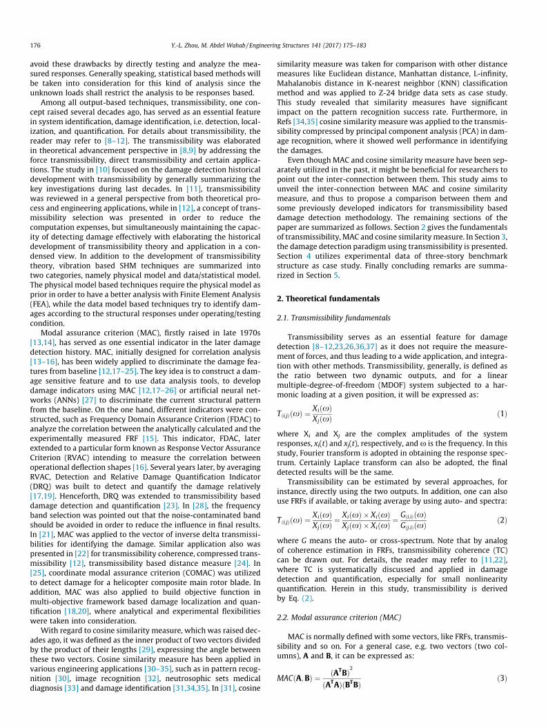
2.3. Cosine similarity measure

Cosine similarity measure aims to illustrate the angle betweentwo vectors, A and B, and it is expressed as:

CosðA;BÞ ¼ ATBjAjjBj ð4Þ

where Cos 2[�1, 1]. When Cos equals to ‘1’, it means that A and Bhold the same direction, while ‘�1’ means that A and B hold theopposite direction. A clear description for the angle is depicted inFig. 1.

2.4. Interrelation between MAC and cosine similarity measure

In order to demonstrate the interrelation between MAC andcosine similarity measure, it is better to calculate the square ofcosine measure. As expressed in Eq. (5), it is proved that the squareof cosine measure is MAC:

CosðA;BÞ2 ¼ ATBjAjjBj

!2

¼ ðATBÞ2

ðATAÞðBTBÞ ¼ MACðA;BÞ ð5Þ

From Eq. (5), it is possible to explain why MAC 2[0,1], i.e. thereason is that Cos2[�1, 1]. And this argument could also explainthat why ‘1 – MAC’ can be objective function in [18,20], since 1-MAC will be sine2, which also hold the value 2[0, 1]. In addition,using the same argument can explain why as damage increases,MAC does not harmonically increases [21].

Taking a as the angle between two vectors A and B, then a 2[0,2p] and the MAC indicator have three tendency changing points,namely ‘p/2’, ‘p’, ‘3p/2’. MAC does not decrease harmonically ver-sus the increase of angle between the two vectors since these threetendency changing points will act as critical values between twotendencies. For instance, when the angle increase from ‘0’ to‘p/2’, MAC will decrease from ‘1’ to ‘0’, and from ‘p/2’ to ‘p’, MACwill increase from ‘0’ to ‘1’. Therefore, in this study, ‘p/2’ is calledtendency changing point. Note that since the angle between thetwo vectors hold [0, 2p], then cosine will solely have one tendencychanging point at p, then from ‘0’ to ‘p’, cosine measure decreasesfrom ‘1’ to ‘�1’ harmonically versus the increase of angle betweentwo vectors. While it increases from ‘�1’ to ‘1’ versus the increaseof angle between two vectors from ‘p’ to ‘2p’. Regarding patternrecognition, all patterns will be recognized from the baseline,namely if the angle between the current pattern and the baselineexists, then it will be identified. Note that the angle ‘p’ theoretically

x

y

z

A

B

Angle(A, B)

Fig. 1. The angle between vector A and B measured by cosine similarity measure.

speaking, will be impossible to see in MAC as MAC = 1, while cosinesimilarity can figure it out as it is ‘�1’.

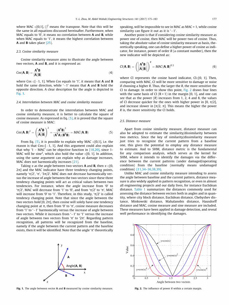
Another point is that if considering cosine similarity measure aspower one of cosine, then MAC will be power two of cosine. Thus,taking the absolute value of cosine similarity measure as basis, the-oretically speaking, one can define a higher power of cosine as indi-cator, for instance, power of order R (a constant number), then thenew indicator will be depicted as:

CIðA;BÞ ¼ ATBjAjjBj

����������

!R

¼ MACðA;BÞR=2 ð6Þ

where CI represents the cosine based indicator, CI2[0, 1]. Then,comparing with MAC, CI will be more sensitive to damage or noiseif choosing a higher R. Thus, the larger the R, the more sensitive theCI to damage. In order to show this point, Fig. 2 draws four lineswith the same basis of CI (R = 1) in the margin [0, 1], and one cansee that as the power (R) increases from 1, 2, 4 and 8, the valuesof CI decrease quicker for the ones with higher power in [0, p/2],and increase slower in [p/2, p]. This means the higher the powerR is, the more sensitivity the CI holds.

2.5. Distance measure

Apart from cosine similarity measure, distance measure canalso be adopted to estimate the similarity/dissimilarity betweentwo metrics. Since the key of similarity/dissimilarity measurejust tries to recognize the current pattern from a baselineone, this gives the potential to employ any distance measureto estimate. And to SHM, distance metric is the fundamentalfor any comparison analysis, which serves as the kernel forSHM, where it intends to identify the damages via the differ-ence between the current patterns (under damaged/operatingcondition) from the baseline (normally means undamagedcondition) [11,34–36,38,39].

Unlike MAC and cosine similarity measure intending to assessthe angle between baseline and the current pattern, distance mea-sure is also widely applied in pattern recognition, or even in almostall engineering projects and our daily lives, for instance Euclideandistance. Table 1 summarizes the distances commonly used forassessing the distance between vectors both in angles and in quan-tity, where city block distance, Euclidean distance, Chebyshev dis-tance, Minkowski distance, Mahalanobis distance, Hausdorffdistance and MAC, cosine measure and sine measure are included.These measures have been applied in damage detection, and revealwell performance in identifying the damages.

0 0.5 1 1.5 2 2.5 30

0.2

0.4

0.6

0.8

Angle between two vectors

Val

ue

y=cos(x)4y=cos(x)8

y=cos(x)2

y=cos(x)

Fig. 2. The influence of power R within a certain margin.

Table 1Summary for distance measure between vectors.

Distance between vectorsNo. Quantitative distance Angle distance

1 City block distance [12] Cosine measure [34,35]2 Euclidean distance [36] Sine measure3 Chebyshev distance [12] MAC [12–14,23,28]4 Minkowski distance [12,35]5 Mahalanobis distance [12,36]6 Hausdorff distance [34]

178 Y.-L. Zhou, M. Abdel Wahab / Engineering Structures 141 (2017) 175–183

3. Damage detection methodology

For damage detection, as discussed above, the general proce-dure is to construct damage sensitive indicators, which will be fur-ther employed to identify damages. Certainly kinds of sensitiveindicators may be constructed, however, the commonest one willstill be MAC, cosine similarity measure and so on. For two data setsTu and Td representing transmissibility under undamaged stateand damaged state, then corresponding damage indicators can becalculated as follows:

3.1. MAC

MACðTd;TuÞ ¼ðTdÞTðTuÞ� �2

ððTdÞTðTdÞÞ ðTuÞTðTuÞ� � ð7Þ

3.2. Cosine similarity measure

Cos Td;Tu� �

¼Td� �T

Tu� �Td��� ��� Tu�� �� ð8Þ

Note that Cos2[�1, 1], for damage detection, since the idea isonly to discriminate the damaged patterns from the baseline, itwill be sufficient to use the absolute value of cosine measure.And certainly, theoretically speaking, MAC will fail to detect thecase if the cosine measure equals to ‘�1’, i.e. the two vectors arein opposite direction, as in this case, MAC will also hold the value‘1’ considering the state to be undamaged as illustrated previously.For engineering application, changing the segment of data sets cansolve this. Then, it will be possible to compare MAC and Cosinebased indicator (CI), which is expressed as:

CIðTd;TuÞ ¼ ðTdÞTðTuÞjTdjjTuj

����������R

¼ MACðTd;TuÞR=2 ð9Þ

where CI2[0, 1]. One may select different R values for checking thesensitivity of CI in damage detection in comparison to MAC and Cos.

Another indicator based on MAC is illustrated as transmissibil-ity damage indicator (TDI) [23], which is defined as:

TDIm ¼ 1Nk

XNk

k¼1

PNii¼1

PNj

j¼1Tmij ðkDxÞTr

ijðkDxÞT��� ���2PNi

i¼1

PNj

j¼1Tmij ðkDxÞTm

ij ðkDxsÞT� � PNi

i¼1

PNj

j¼1TrijðkDxÞTr

ijðkDxsÞT� �

ð10Þwhere m represents mth measurement, Dx means the frequencyresolution, k means the frequency index, Nk, Ni, Nj are the numberof frequency lines of the transmissibility, number of coordinatesmeasured and number of excitations measured, respectively [23].()r means the reference measured data, i.e. the data measured underundamaged condition.

By analog of the CI definition, one may also extend TDI (ETDI)definition into a general one, which can be illustrated as:

ETDIm ¼ 1Nk

XNk

k¼1

PNii¼1

PNj

j¼1Tmij ðkDxÞTr

ijðkDxÞT��� ���Q

PNii¼1

PNj

j¼1Tmij ðkDxÞTm

ij ðkDxÞT� � PNi

i¼1

PNj

j¼1TrijðkDxÞTr

ijðkDxÞT� �� �Q=2

ð11Þwhere Q means the power of TDI. And Q = 1 means cosine basedTDI; Q = 2 means TDI; Q = 3 means enhanced TDI, where the sensi-tivity of ETDI will be higher than TDI. The higher the Q value is, themore sensitive the ETDI will be. Note this is an empirical setting of Rand Q relying on the engineer’s experience.

Note that FRFs have been commonly used in previous investiga-tions for damage detection. In this study, FRFs are also employed inCI and ETDI indicators for comparison with transmissibility basedCI and ETDI.

The damage detection procedure can be illustrated in a three-step paradigm.

Step 1: Transmissibility estimation. In this step, transmissibilitywill be estimated from structural dynamic responses using Eq.(2);Step 2: Damage indicators derivation. From Eqs. (10) and (11)damage indicators will be derived;Step 3: Damage prediction. Finally, one may predict the dam-ages from the results of the indicators in accordance to engi-neers’ experience.

4. Experimental validation

4.1. Model description

In order to verify the developed damage detection procedureand the two newly developed damage indicators, an open sourceof three-story floor structure tested in Los Alamos Lab is adopted[11,22,40–43] as shown in Fig. 3. The data can be downloaded from(http://www.lanl.gov/projects/national-security-education-center/engineering/ei-software-download/thanks.php). The reason toadopt this structure as a case study is that it has been well inves-tigated in previous work [11,22,40–43], and proves to be a repre-sentative structural model in real engineering. Four aluminumcolumns (17.7 � 2.5 � 0.6 cm3) are adopted to connect the aboveand below aluminum plates (30.5 � 30.5 � 2.5 cm3). The structureis installed on rails allowing solely x-direction movement. A centercolumn from the top floor is designed to generate nonlinearitywhen it hits the bumper. A shaker at the center of the base floorexcites the structure. Four accelerometers (Channels 2–5) are usedto record the horizontal movement of each floor from base, first,second and third floor, and load cell (Channel 1) is adopted torecord the excitation. All the time-domain series are measuredfor 17 different structural conditions as described in Table 2, wherefor each state, 50 measurements are recorded separately. Furtherinformation about this experiment, the reader may refer to[11,22,40–43], all information including the experiment descrip-tion illustrated above can be found.

4.2. Results and discussion

Results for the proposed damage detection procedure and thenewly derived damage indicators, are given and discussed indetails hereinafter.

4.2.1. Applicability of transmissibility in damage detectionFigs. 4 and 5 illustrate the transmissibility T(5, 3) and T(4, 3) for

the State #1, #2, #6 and #10, respectively. Note here T(5, 3) means

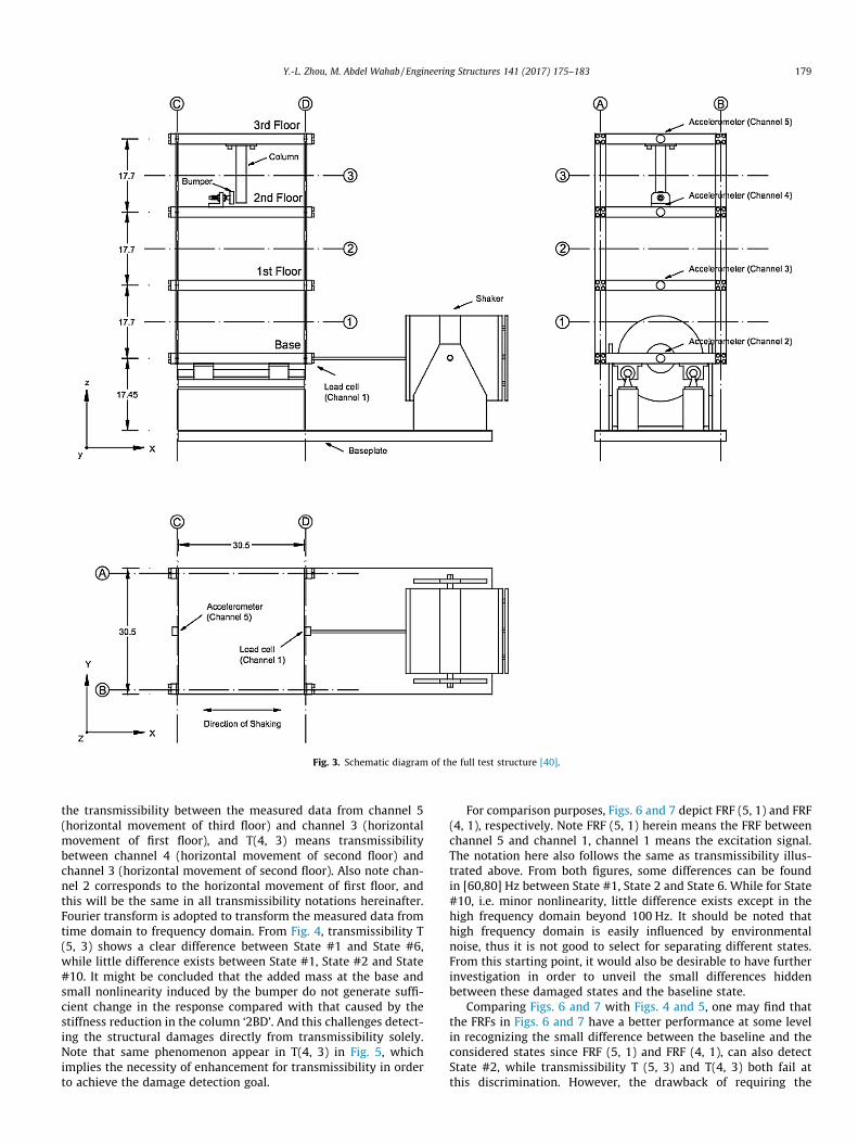
Fig. 3. Schematic diagram of the full test structure [40].

Y.-L. Zhou, M. Abdel Wahab / Engineering Structures 141 (2017) 175–183 179

the transmissibility between the measured data from channel 5(horizontal movement of third floor) and channel 3 (horizontalmovement of first floor), and T(4, 3) means transmissibilitybetween channel 4 (horizontal movement of second floor) andchannel 3 (horizontal movement of second floor). Also note chan-nel 2 corresponds to the horizontal movement of first floor, andthis will be the same in all transmissibility notations hereinafter.Fourier transform is adopted to transform the measured data fromtime domain to frequency domain. From Fig. 4, transmissibility T(5, 3) shows a clear difference between State #1 and State #6,while little difference exists between State #1, State #2 and State#10. It might be concluded that the added mass at the base andsmall nonlinearity induced by the bumper do not generate suffi-cient change in the response compared with that caused by thestiffness reduction in the column ‘2BD’. And this challenges detect-ing the structural damages directly from transmissibility solely.Note that same phenomenon appear in T(4, 3) in Fig. 5, whichimplies the necessity of enhancement for transmissibility in orderto achieve the damage detection goal.

For comparison purposes, Figs. 6 and 7 depict FRF (5, 1) and FRF(4, 1), respectively. Note FRF (5, 1) herein means the FRF betweenchannel 5 and channel 1, channel 1 means the excitation signal.The notation here also follows the same as transmissibility illus-trated above. From both figures, some differences can be foundin [60,80] Hz between State #1, State 2 and State 6. While for State#10, i.e. minor nonlinearity, little difference exists except in thehigh frequency domain beyond 100 Hz. It should be noted thathigh frequency domain is easily influenced by environmentalnoise, thus it is not good to select for separating different states.From this starting point, it would also be desirable to have furtherinvestigation in order to unveil the small differences hiddenbetween these damaged states and the baseline state.

Comparing Figs. 6 and 7 with Figs. 4 and 5, one may find thatthe FRFs in Figs. 6 and 7 have a better performance at some levelin recognizing the small difference between the baseline and theconsidered states since FRF (5, 1) and FRF (4, 1), can also detectState #2, while transmissibility T (5, 3) and T(4, 3) both fail atthis discrimination. However, the drawback of requiring the

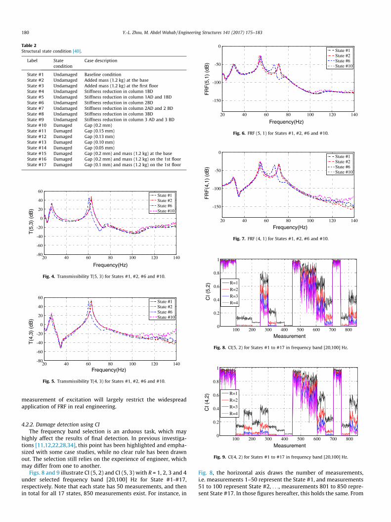
Table 2Structural state condition [40].

Label Statecondition

Case description

State #1 Undamaged Baseline conditionState #2 Undamaged Added mass (1.2 kg) at the baseState #3 Undamaged Added mass (1.2 kg) at the first floorState #4 Undamaged Stiffness reduction in column 1BDState #5 Undamaged Stiffness reduction in column 1AD and 1BDState #6 Undamaged Stiffness reduction in column 2BDState #7 Undamaged Stiffness reduction in column 2AD and 2 BDState #8 Undamaged Stiffness reduction in column 3BDState #9 Undamaged Stiffness reduction in column 3 AD and 3 BDState #10 Damaged Gap (0.2 mm)State #11 Damaged Gap (0.15 mm)State #12 Damaged Gap (0.13 mm)State #13 Damaged Gap (0.10 mm)State #14 Damaged Gap (0.05 mm)State #15 Damaged Gap (0.2 mm) and mass (1.2 kg) at the baseState #16 Damaged Gap (0.2 mm) and mass (1.2 kg) on the 1st floorState #17 Damaged Gap (0.1 mm) and mass (1.2 kg) on the 1st floor

20 40 60 80 100 120 140-80

-60

-40

-20

0

20

40

60

Frequency(Hz)

T(5

,3)

(dB

)

State #1State #2State #6State #10

Fig. 4. Transmissibility T(5, 3) for States #1, #2, #6 and #10.

20 40 60 80 100 120 140-80

-60

-40

-20

0

20

40

60

Frequency(Hz)

T(4

,3)

(dB

)

State #1State #2State #6State #10

Fig. 5. Transmissibility T(4, 3) for States #1, #2, #6 and #10.

20 40 60 80 100 120 140

-150

-100

-50

0

Frequency(Hz)

FR

F(5

,1)

(dB

)

State #1State #2State #6State #10

Fig. 6. FRF (5, 1) for States #1, #2, #6 and #10.

20 40 60 80 100 120 140

-150

-100

-50

0

Frequency(Hz)

FR

F(4

,1)

(dB

)

State #1State #2State #6State #10

Fig. 7. FRF (4, 1) for States #1, #2, #6 and #10.

100 200 300 400 500 600 700 8000

0.2

0.4

0.6

0.8

1

Measurement

CI (

5,2)

R=1

R=2

R=3

R=4

Fig. 8. CI(5, 2) for States #1 to #17 in frequency band [20,100] Hz.

0.4

0.6

0.8

1

CI (

4,2)

R=1

R=2

R=3

180 Y.-L. Zhou, M. Abdel Wahab / Engineering Structures 141 (2017) 175–183

measurement of excitation will largely restrict the widespreadapplication of FRF in real engineering.

100 200 300 400 500 600 700 8000

0.2

Measurement

R=4

Fig. 9. CI(4, 2) for States #1 to #17 in frequency band [20,100] Hz.

4.2.2. Damage detection using CIThe frequency band selection is an arduous task, which may

highly affect the results of final detection. In previous investiga-tions [11,12,22,28,34], this point has been highlighted and empha-sized with some case studies, while no clear rule has been drawnout. The selection still relies on the experience of engineer, whichmay differ from one to another.

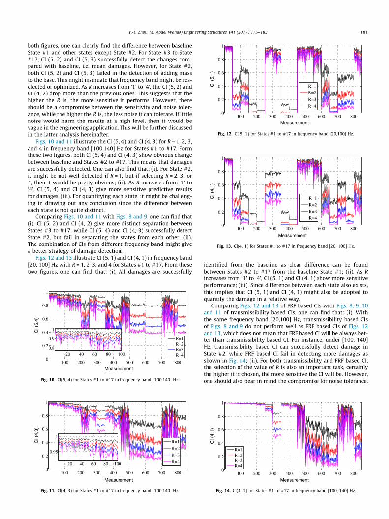
Figs. 8 and 9 illustrate CI (5, 2) and CI (5, 3) with R = 1, 2, 3 and 4under selected frequency band [20,100] Hz for State #1-#17,respectively. Note that each state has 50 measurements, and thenin total for all 17 states, 850 measurements exist. For instance, in

Fig. 8, the horizontal axis draws the number of measurements,i.e. measurements 1–50 represent the State #1, and measurements51 to 100 represent State #2, . . ., measurements 801 to 850 repre-sent State #17. In those figures hereafter, this holds the same. From

100 200 300 400 500 600 700 8000

0.2

0.4

0.6

0.8

1

Measurement

CI (

5,1)

R=1

R=2

R=3

R=4

Fig. 12. CI(5, 1) for States #1 to #17 in frequency band [20,100] Hz.

100 200 300 400 500 600 700 8000

0.2

0.4

0.6

0.8

1

Measurement

CI (

4,1)

R=1

R=2

R=3

R=4

Fig. 13. CI(4, 1) for States #1 to #17 in frequency band [20, 100] Hz.

Y.-L. Zhou, M. Abdel Wahab / Engineering Structures 141 (2017) 175–183 181

both figures, one can clearly find the difference between baselineState #1 and other states except State #2. For State #3 to State#17, CI (5, 2) and CI (5, 3) successfully detect the changes com-pared with baseline, i.e. mean damages. However, for State #2,both CI (5, 2) and CI (5, 3) failed in the detection of adding massto the base. This might insinuate that frequency band might be res-elected or optimized. As R increases from ‘1’ to ‘4’, the CI (5, 2) andCI (4, 2) drop more than the previous ones. This suggests that thehigher the R is, the more sensitive it performs. However, thereshould be a compromise between the sensitivity and noise toler-ance, while the higher the R is, the less noise it can tolerate. If littlenoise would harm the results at a high level, then it would bevague in the engineering application. This will be further discussedin the latter analysis hereinafter.

Figs. 10 and 11 illustrate the CI (5, 4) and CI (4, 3) for R = 1, 2, 3,and 4 in frequency band [100,140] Hz for States #1 to #17. Formthese two figures, both CI (5, 4) and CI (4, 3) show obvious changebetween baseline and States #2 to #17. This means that damagesare successfully detected. One can also find that: (i). For State #2,it might be not well detected if R = 1, but if selecting R = 2, 3, or4, then it would be pretty obvious; (ii). As R increases from ‘1’ to‘4’, CI (5, 4) and CI (4, 3) give more sensitive predictive resultsfor damages. (iii). For quantifying each state, it might be challeng-ing in drawing out any conclusion since the difference betweeneach state is not quite distinct.

Comparing Figs. 10 and 11 with Figs. 8 and 9, one can find that(i). CI (5, 2) and CI (4, 2) give more distinct separation betweenStates #3 to #17, while CI (5, 4) and CI (4, 3) successfully detectState #2, but fail in separating the states from each other; (ii).The combination of CIs from different frequency band might givea better strategy of damage detection.

Figs. 12 and 13 illustrate CI (5, 1) and CI (4, 1) in frequency band[20, 100] Hz with R = 1, 2, 3, and 4 for States #1 to #17. From thesetwo figures, one can find that: (i). All damages are successfully

100 200 300 400 500 600 700 8000

0.2

0.4

0.6

0.8

1

Measurement

CI (

5,4)

R=1R=2R=3R=420 40 60 80 100

0.8

0.9

1

Fig. 10. CI(5, 4) for States #1 to #17 in frequency band [100,140] Hz.

100 200 300 400 500 600 700 8000

0.2

0.4

0.6

0.8

1

Measurement

CI (

4,3)

R=1

R=2

R=3

R=420 40 60 80 100

0.95

1

Fig. 11. CI(4, 3) for States #1 to #17 in frequency band [100,140] Hz.

identified from the baseline as clear difference can be foundbetween States #2 to #17 from the baseline State #1; (ii). As Rincreases from ‘1’ to ‘4’, CI (5, 1) and CI (4, 1) show more sensitiveperformance; (iii). Since difference between each state also exists,this implies that CI (5, 1) and CI (4, 1) might also be adopted toquantify the damage in a relative way.

Comparing Figs. 12 and 13 of FRF based CIs with Figs. 8, 9, 10and 11 of transmissibility based CIs, one can find that: (i). Withthe same frequency band [20,100] Hz, transmissibility based CIsof Figs. 8 and 9 do not perform well as FRF based CIs of Figs. 12and 13, which does not mean that FRF based CI will be always bet-ter than transmissibility based CI. For instance, under [100, 140]Hz, transmissibility based CI can successfully detect damage inState #2, while FRF based CI fail in detecting more damages asshown in Fig. 14; (ii). For both transmissibility and FRF based CI,the selection of the value of R is also an important task, certainlythe higher it is chosen, the more sensitive the CI will be. However,one should also bear in mind the compromise for noise tolerance.

100 200 300 400 500 600 700 8000

0.2

0.4

0.6

0.8

1

Measurement

CI (

4,1)

R=1R=2R=3R=4

Fig. 14. CI(4, 1) for States #1 to #17 in frequency band [100, 140] Hz.

100 200 300 400 500 600 700 8000

0.2

0.4

0.6

0.8

1

Measurement

ET

DI (

FR

F)

Q=1Q=6Q=7Q=820 40 60 80 100

0.98

0.99

1

Fig. 18. FRF based ETDI for States #1 to #17 with Q = 1, 6, 7, 8.

182 Y.-L. Zhou, M. Abdel Wahab / Engineering Structures 141 (2017) 175–183

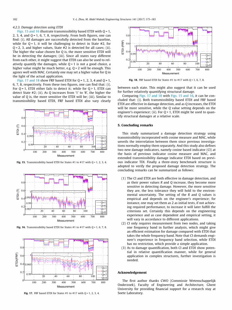
4.2.3. Damage detection using ETDIFigs. 15 and 16 illustrate transmissibility based ETDI with Q = 1,

2, 3, 4, and Q = 1, 6, 7, 8, respectively. From both figures, one canfind: (i). All damages are successfully detected from the baseline,while for Q = 1, it will be challenging to detect in State #2, forQ = 2, 3, and higher values, State #2 is detected for all cases; (ii).The higher the value chosen for Q is, the more sensitive ETDI willbe in detecting the damages; (iii). Since all states vary differentfrom each other, it might suggest that ETDI can also be used to rel-atively quantify the damages, while Q = 1 is not a good choice, ahigher value might be much better, e.g. Q = 2 will be enough. Thisagrees well with MAC. Certainly one may set a higher value for Q inthe light of the actual application.

Figs. 17 and 18 show FRF based ETDI for Q = 1, 2, 3, 4 and Q = 1,6, 7, 8, respectively. From these two figures, one can find that: (i).For Q = 1, ETDI either fails to detect it; while for Q > 1, ETDI candetect State #2; (ii). As Q increases from ‘1’ to ‘8’, the higher thevalue of Q is, the more sensitive the ETDI will be; (iii). Similar totransmissibility based ETDI, FRF based ETDI also vary clearly

100 200 300 400 500 600 700 8000

0.2

0.4

0.6

0.8

1

Measurement

ET

DI (

T)

Q=1Q=2Q=3Q=420 40 60 80 100

0.99

0.995

1

Fig. 15. Transmissibility based ETDI for States #1 to #17 with Q = 1, 2, 3, 4.

100 200 300 400 500 600 700 8000

0.2

0.4

0.6

0.8

1

Measurement

ET

DI (

T)

Q=1Q=6Q=7Q=820 40 60 80 100

0.985

0.99

0.995

1

Fig. 16. Transmissibility based ETDI for States #1 to #17 with Q = 1, 6, 7, 8.

100 200 300 400 500 600 700 8000

0.2

0.4

0.6

0.8

1

Measurement

ET

DI(

FR

F)

Q=1Q=2Q=3Q=420 40 60 80 100

0.99

0.995

1

Fig. 17. FRF based ETDI for States #1 to #17 with Q = 1, 2, 3, 4.

between each state. This might also suggest that it can be usedfor further relatively quantifying structural damage.

Comparing Figs. 17 and 18 with Figs. 15 and 16, it can be con-cluded that: (i). Both transmissibility based ETDI and FRF basedETDI are effective in damage detection, and as Q increases, the ETDIwill be more sensitive, while the Q value setting depends on theengineer’s experience; (ii). For Q > 1, ETDI might be used to quan-tify structural damages at a relative scale.

5. Concluding remarks

This study summarized a damage detection strategy usingtransmissibility incorporated with cosine measure and MAC, whileunveils the interrelation between them since previous investiga-tions normally employ them separately. And this study also definestwo new damage indicators, namely cosine based indicator (CI) atthe basis of previous indicator cosine measure and MAC, andextended transmissibility damage indicator ETDI based on previ-ous indicator TDI. Finally a three-story benchmark structure isadopted to verify the proposed damage detection strategy. Theconcluding remarks can be summarized as follows:

(1) The CI and ETDI are both effective in damage detection, andas their power values R and Q increase, they become moresensitive in detecting damage. However, the more sensitivethey are, the less tolerance they will hold to the environ-mental uncertainty. The setting of the R and Q values isempirical and depends on the engineer’s experience; forinstance, one may set them as 2 as initial tests, if not achiev-ing required performance, to increase it will later fulfill thecriterions set. Certainly this depends on the engineeringexperience and as case dependent and empirical setting, itwill vary in accordance to different applications.

(2) CI only requires measurement from two nodes, and takingone frequency band in further analysis, which might givean efficient estimation for damage compared with ETDI thattakes the whole frequency band. Note that CI demands engi-neer’s experience in frequency band selection, while ETDIhas no restriction, which provide a simple application.

(3) As to damage quantification, both CI and ETDI show poten-tial in relative quantification manner, while for generalapplication in complex structures, further investigation isneeded.

Acknowledgement

The first author thanks CWO (Commissie WetenschappelijkOnderzoek), Faculty of Engineering and Architecture, GhentUniversity for providing financial support for a research stay atSoete Laboratory.

Y.-L. Zhou, M. Abdel Wahab / Engineering Structures 141 (2017) 175–183 183

References

[1] Sohn H, Farrar CR, Hemez FM, Shunk DD, Stinemates SW, Nadler BRand Czarnecki JJ 2004 A review of structural health monitoring literaturefrom 1996–2001 Technical Report LA-13976-MS Los Alamos NationalLaboratory.

[2] Montalvao D, Maia NMM, Ribeiro AMR. A review of vibration-based structuralhealth monitoring with special emphasis on composite materials. Shock VibrDigest 2006;38(4):295–324.

[3] Zhou Y-L, Maia NMM, Sampaio R, Wahab MA. Structural damage detectionusing transmissibility together with hierarchical clustering analysis andsimilarity measure. Struct Health Monit 2016. http://dx.doi.org/10.1177/1475921716680849.

[4] Khatir S, Belaidi I, Serra R, Abdel Wahab M, Khatir T. Numerical study for singleand multiple damage detection and localization in beam-like structures usingBAT algorithm. J Vibroeng 2016;18(1):202–13.

[5] Khatir A, Tehami M, Khatir S, Abdel Wahab M. Multiple damage detection andlocalization in beam-like and complex structures using co-ordinate modalassurance criterion combined with firefly and genetic algorithms. J Vibroeng2016;18(8):5063–73.

[6] Gillich G-R, Praisach Z-I, Abdel Wahab M, Gillich N, Mituletu IC, Nitescu C 2016Free vibration of a perfectly clamped-free beam with stepwise eccentricdistributed masses Shock and Vibration 2016(Article ID 2086274) 10 pages;doi: 10.1155/2016/2086274.

[7] Khatir S, Belaidi I, Serra R, Abdel Wahab M, Khatir T. Damage detection andlocalization in composite beam structures based on vibration analysis.Mechanika 2015;21(6):472–9.

[8] Maia NMM, Urgueira APV, Almeida RAB. Whys and Wherefores ofTransmissibility Vibration Analysis and Control – New Trends andDevelopments. InTech; 2011. ISBN 978-953-307-433-977, 364 pages, pp.197–216.

[9] Maia NMM, Lage YE, Neves MM. Recent Advances on Force Identification inStructural Dynamics Advances in Vibration Engineering and StructuralDynamics. InTech; 2012. ISBN 978-953-951-0845-0840, 0378 pages, pp.0103–0132.

[10] Chesne S, Deraemaeker A. Damage localization using transmissibilityfunctions: a critical review. Mech Syst Signal Process 2013;38(2):569–84.

[11] Zhou YL. Structural health monitoring by using transmissibility PhD thesis,2015.

[12] Zhou Y-L, Maia NMM, Wahab MA. Damage detection using transmissibilitycompressed by principal component analysis enhanced with distancemeasure. J Vib Control 2016. http://dx.doi.org/10.1177/1077546316674544.

[13] Allemang RJ, Brown DL, A Correlation Coefficient for Modal Vector AnalysisProceedings of the 1st International Modal Analysis Conference, 1982, 110–116.

[14] Allemang RJ. The Modal Assrance Criterion (MAC): Twenty Years of Use andAbse Journal of Sound and Vibration August 14–21, 2003.

[15] Pascal R, Golinval JC, Razeto M. A Frequency Domain Correlation Technique forModel Correlation and Updating Proceedings of the 15th International ModalAnalysis Conference – IMAC 587–592, 1997.

[16] Heylen W, Lammens S, Sas P. Modal Analysis Theory and Testing KU Leuven-PMA Belgium, Section A.6, 1998.

[17] Maia NMM, Ribeiro AMR, Fontul M, Montalvao D, Sampaio RPC. Using thedetection and relative damage quantification indicator (DRQ) withtransmissibility. In: Garibaldi L, Surace C, Holford K, Ostachowicz WM,editors. Damage Assessment of Structures Vii. Key Engineering Materials.3472007. p. 455–460.

[18] Perera R, Ruiz A, Manzano C. An evolutionary multiobjective framework forstructural damage localization and quantification. Eng Struct2007;29:2540–50.

[19] Sampaio R, Maia N. Strategies for an efficient indicator of structural damage.Mech Syst Signal Process 2009;23:1855–69.

[20] Perera R, Ruiz A, Manzano C. Performance assessment of multicriteria damageidentification genetic algorithms. Comput Struct 2009;87:120–7.

[21] Zhou YL, Perera R, Sevillano E. Damage identification from power spectrumdensity transmissibility Proceedings of the 6th European Workshop onStructural Health Monitoring Dresden, Germany, July 2012, 2012.

[22] Zhou Y-L, Figueiredo E, Maia NMM, Perera R. Damage detection andquantification using transmissibility coherence analysis Shock and Vibration2015(Article ID 290714), 2015.

[23] Sampaio R, Maia N, Almeida RAB, Urgueira APV. A simple damage detectionindicator using operational deflection shapes. Mech Syst Signal Process2015;72–73:629–41.

[24] Zhou Y-L, Wahab MA. Rapid early damage detection using transmissibilitywith distance measure analysis under unknown excitation in long-term healthmonitoring. J Vibroeng 2016;18(7):4491–9.

[25] Santos FLM, Peeters B, Auweraer H, Goes LCS and Desmet W, Vibration-baseddamage detection for a composite helicopter main rotor blade Case studies inMechnical Systems and Signal Processing 3(22–27), 2016.

[26] Zhou Y-L, Wahab MA, Perera R. Damage detection by transmissibilityconception in beam-like structures. Int J Fract Fatigue Wear 2015;3:254–9.

[27] Zhou YL, Perera R. Transmissibility based damage assessment by intelligentalgorithm Proceedings of the 9th European Conference on Structural Dynamics(EURODYN 2014) Oporto, Portugal, June 2014, 2014.

[28] Zhou Y-L, Wahab MA, Figueiredo E, Maia NMM, Sampaio R, Perera R. Singleside damage simulations and detection in beam-like structures. J Phys: ConfSer 2015;628:012036.

[29] Ye J. Cosine similarity measures for intuitionistic fuzzy sets and theirapplications. Math Comput Model 2011;53:91–7.

[30] Junjie Wua SZ, Liu Hongfu, Xia Guoping. Cosine interesting pattern discovery.Inf Sci 2012;184:176–95.

[31] Liu W, Chen B, Swartz RA, Investigation of Time Series Representations andSimilarity Measures for Structural Damage Pattern Recognition The ScientificWorld Journal 2013 Article ID 248349, 248313 pages, 2013.

[32] Ye J. Improved cosine similarity measures of simplified neutrosophic sets formedical diagnoses. Artif Intell Med 2015;63:171–9.

[33] Xia P, Zhang L, Li F. Learning similarity with cosine similarity ensemble. Inf Sci2015;307:39–52.

[34] Zhou Y-L, Maia NMM, Sampaio R, Wahab MA, Structural damage detectionusing transmissibility together with hierarchical clustering analysis andsimilarity measure. Struct Health Monit Int J, in press, https://dx.doi.org/10.1177/1475921716680849.

[35] Zhou Y-L, Maia NMM, Sampaio R, Qian XD, Wahab MA. Damage detection viatransmissibility enhanced with similarity analysis and principal componentanalysis. In: Proceedings of the 2016 Leuven Conference on Noise andVibration Engineering (ISMA 2016) Leuven, Belgium, September 2016, 2016.

[36] Zhou Y-L, Figueiredo E, Maia NMM, Sampaio R, Perera R. Damage detection instructures using a transmissibility-based Mahalanobis distance. Struct ControlHealth Monit 2015;22:1209–22.

[37] Zhou Y-L, Figueiredo E, Maia NMM, Perera R. Damage detection usingtransmissibility coherence Proceedings of the International Conference onStructural Engineering Dynamics (ICEDyn 2015) Lagos, Algarve, Portugal, June2015, 2015.

[38] Worden K, Manson G, Fieller NRJ. Damage detection using outliner analysis. JSound Vib 2000;229(3):647–67.

[39] Figueiredo E, Cross E. Linear approaches to modeling nonlinearities in long-term monitoring of bridges. J Civ Struct Health Monit 2013;3(3):187–94.

[40] http://www.lanl.gov/projects/national-security-education-center/engineering/ei-software-download/thanks.php.

[41] Figueiredo E, Park G, Figueiras J, Farrar CR, Worden K. Structural healthmonitoring algorithm comparisons using standard data sets Los AlamosNational Laboratory Report LA-14393 Los Alamos National Laboratory, 2009.

[42] Figueiredo E. Damage Identification in Civil Engineering Infrastructure underOperational and Environmental Conditions PhD thesis Porto University,Portugal, 2010.

[43] Figueiredo E, Flynn E. Three-story building structure to detect nonlineareffects, 2013 http://wwwlanlgov/projects/national-security-education-center/engineering/ei-software-download/thanksphp.