Application of TAPM (v.1) in Swedish West Coast ... . Deliang Chen. 1, 2, Tijian Wang. 1, 2, Marie Haeger-Eugensson. 1, Christine Achberger. 2, Katarina Borne. 2 . 1. IVL Swedish Environmental

REPORT

Application of TAPM (v.1) in Swedish West Coast:

validation during 1999-2000

1IVL Swedish Environmental Research Ltd 2Earth Sciences Centre, Gothenburg University

The report approved: 2002-10-25

Karin Sjöberg Enhetschef

M Deliang Chen1,2, Tijian Wang1,2, Marie Haeger-Eugensson1, Christine Achberger2, Katarina Borne2

B2164 2002

Organization

IVL Swedish Environmental Research Institute Ltd. Report Summary Project title

Address P.O. Box 53021 SE-400 14 Göteborg Project sponsor

Telephone +46 (0)31-725 62 00

Author Deliang Chen1,2, Tijian Wang1,2, Marie Haeger-Eugensson1, Christine Achberger2, Katarina Borne2

1IVL Swedish Environmental Research Ltd 2Earth Sciences Centre, Gothenburg University Title and subtitle of the report Application of TAPM (v.1) in Swedish West Coast: validation during 1999-2000 Summary TAPM, The Air Pollution Model, was developed by Australian CSIRO Atmospheric Research Division. It is a 3-D meteorological and chemical model for air pollution studies. TAPM has been applied by IVL since 1999. To our knowledge TAPM has not yet been tested against observations in Sweden before. This report summarises an extensive simulation during 1999-2000 with the Swedish West Coast in focus. First it gives a brief description of TAPM. Then the details of the simulation including set-up of the model and choices made in modelling are explained. Three nestings were used to come down to the finest resolution of 1 km. The modelled results in terms of the surface air temperature and wind, as well as vertical profiles of wind, have been compared with available observations to examine TAPM’s performance for local meteorology that is often central to air pollution modelling in coastal areas. The NCDC surface meteorological data and sound radar (SODAR) data collected by Luft i Väst were used for the comparison. Investigations have shown that the model performs well in simulating air temperature and wind, which are the two most important fields to drive air pollution modelling. Also, TAPM was confirmed to have strong ability in simulating thermally driven meso-scale systems, such as sea-land breeze and urban heat island effect. It is thus concluded that TAPM is a very useful tool for local meteorological air pollution applications. Finally, some practical aspects of the future use of TAPM are commented and several useful tools for post-processing were developed and presented. Keyword TAPM model, Validation meteorological modelling, Swedish west coast

Bibliographic data

IVL Report B2164 The report can be ordered via Homepage: www.ivl.se, e-mail: [email protected], fax+46 (0)8-598 563 90, or via IVL, P.O. Box 21060, SE-100 31 Stockholm Sweden

Application of TAPM (v.1) in Swedish West Coast: IVL report B2164 validation during 1999-2000

Contents

Abstract ...............................................................................................................................................2 1. Background .................................................................................................................................1 2. Description of the model system ................................................................................................1

2.1 Essentials of the Model ..........................................................................................................1 2.2. Meteorology model ................................................................................................................2 2.3. Air pollution model ................................................................................................................2 2.4. Graphical user interface .........................................................................................................2

3. Validation of the model system ...................................................................................................3 3.1. Model set-up and methodology ...........................................................................................3 3.2. Observational Data ................................................................................................................3

4.Results...............................................................................................................................................5 4.1. Surface comparison ................................................................................................................5 4.2 Profile comparison ............................................................................................................... 14

5. Model outputs ............................................................................................................................. 30 6. Comments on use of TAPM ..................................................................................................... 30

6.1. Computer requirements ...................................................................................................... 30 6.2 Model limitations .................................................................................................................. 30 6.3. Soil moisture setting ............................................................................................................ 30 6.4. Output processing ............................................................................................................... 31

7. Conclusions ................................................................................................................................. 31 Acknowledgement .......................................................................................................................... 31 Reference .......................................................................................................................................... 31 Appendix 1 The 50 Swedish meteorological stations ................................................................ 32 Appendix 2 Tools developed ........................................................................................................ 34


Abstract TAPM, The Air Pollution Model, was developed by Australian CSIRO Atmospheric Research Division. It is a 3-D meteorological and chemical model for air pollution studies. TAPM has been applied by IVL since 1999. To our knowledge TAPM has not yet been tested against observations in Sweden before. This report summarises an extensive simulation during 1999-2000 with the Swedish West Coast in focus. First it gives a brief description of TAPM. Then the details of the simulation including set-up of the model and choices made in modelling are explained. Three nestings were used to come down to the finest resolution of 1 km. The modelled results in terms of the surface air temperature and wind, as well as vertical profiles of wind, have been compared with available observations to examine TAPM’s performance for local meteorology that is often central to air pollution modelling in coastal areas. The NCDC surface meteorological data and sound radar (SODAR) data collected by Luft i Väst were used for the comparison. Investigations have shown that the model performs well in simulating air temperature and wind, which are the two most important fields to drive air pollution modelling. Also, TAPM was confirmed to have strong ability in simulating thermally driven meso-scale systems, such as sea-land breeze and urban heat island effect. It is thus concluded that TAPM is a very useful tool for local meteorological air pollution applications. Finally, some practical aspects of the future use of TAPM are commented and several useful tools for post-processing were developed and presented.


1

1. Background Mathematical models are powerful tools for studying meteorology, air pollution problems and emission control strategies. Until now, there have been many air quality models developed for different scales ranging from local, urban, regional and global scales. On urban to regional scales, established air quality models, such as RADM, ADOM, STEM, RAINS-ASIA, CALGRID/CALPUFF and MODELS3, have been developed by different research groups in the world. However, most of these models have relatively coarse spatial resolutions and are difficulty to be applied for long-term simulations due to the complex physical and chemical processes involved. Recently, TAPM (The Air Pollution Model) developed by Australian CSIRO Atmospheric Research Division, appeared as an attractive model system since it integrates meteorology and air chemistry (Hurley, 1999b). This model was designed to be run in a nestable way so that the spatial resolution can be as fine as ~100 m. In addition, it can be run for one year or longer, which provides a means to deal with statistics of meteorological and pollutant variables. TAPM has been used and verified for regions in Australia and other parts in the world (e.g. Hurley, 1999a). CSIRO has applied the model to meteorological (and some air pollution) verification studies for Kwinana and the Pilbara (WA), Cape Grim and Launceston (TAS) (Hurley, 1999a), Melbourne (VIC), Newcastle and Sydney (NSW), and Mt Isa (QLD), as well as for Kuala Lumpur (Malaysia). However, to our knowledge, use of TAPM in Europe has not been documented before. For its wide application in environmental impact assessments in Europe and in Sweden, it is necessary to perform a model validation using the observational data. In this report, a comparison will be made between the model results and the measurement to quantify TAPM’s ability and performance for Sweden.

2. Description of the model system

2.1 Essentials of the Model

Air pollution models that can be used to predict pollution concentrations for periods of up to a year, are generally semi-empirical/analytic approaches based on Gaussian plumes or puffs. Typically, these models use either observed data from a surface based meteorological station or a diagnostic wind field model based on available observations. TAPM is different from these approaches in that it solves the fundamental fluid dynamics and scalar transport equations to predict meteorology and pollutant concentration for a range of pollutants important for air pollution applications. It consists of coupled prognostic meteorological and air pollution concentration components, eliminating the need to have site-specific meteorological observations. Instead, the model predicts the flows important to local-scale air pollution transport, such as sea breezes and terrain induced flows, against a background of larger-scale meteorology provided by synoptic analyses. It predicts meteorological and pollution parameters directly (including some photochemistry) on local, city or inter-


2

regional scales. Its output can also be used to drive regulatory models such as ISC, AUSPLUME, DISPMOD, and AUSPUFF.

2.2. Meteorology model

The meteorological component of TAPM is an incompressible, non-hydrostatic, primitive equation model with a terrain-following vertical co-ordinate for three-dimensional simulations. The model solves the momentum equations for horizontal wind components, the incompressible continuity equation for vertical velocity, and scalar equations for potential virtual temperature and specific humidity of water vapour, cloud water and rainwater. Explicit cloud microphysical processes are included. Turbulence kinetic energy and eddy dissipation rates are calculated for determining the turbulence terms and the vertical fluxes. Further, surface energy budget is considered to computer the surface temperature. A vegetative canopy and soil scheme is used at the surface. Radiative fluxes at the surface and at upper levels are also calculated.

2.3. Air pollution model

The air pollution component of TAPM, which uses predicted meteorology and turbulence from the meteorological component, includes three modules. The Eulerian Grid Module (EGM) solves prognostic equations for concentration and for cross-correlation of concentration and virtual potential temperature. The Lagrangian Particle Module (LPM) can be used to represent near-source dispersion more accurately, while the Plume Rise Module is used to account for plume momentum and buoyancy effects for point sources. The model also has gas-phase photochemical reactions based on the Generic Reaction Set, and gas- and aqueous-phase chemical reactions for sulphur dioxide and particles. In addition, wet and dry deposition effects are also included.

2.4. Graphical user interface

The model is driven by a graphical user interface, which is used to: (1) select all model input and configuration options, including access to supplied databases of terrain height, vegetation and soil type (USGS), synoptic-scale meteorology (CSIRO), and sea-surface temperature (NOAA) (2) run the model (3) choose and process model output, including options for visualisation, extraction of time-series, production of static 1-D and 2-D plots and summary statistics using common packages such as EXCEL.


3

3. Validation of the model system

3.1. Model set-up and methodology

Since meteorological factors play an important role in air pollution modeling, it is necessary to verify the model’s performance on meteorology modeling first. For this purpose, TAPM was run with three nestings that have spatial resolution of 9 km, 3 km and 1 km. There were 90*90 grid points in horizontal dimensions (see Figure 1) and 20 levels in vertical (10, 50, 100, 150, 200, 300, 400, 500, 750, 1000, 1250, 1500, 2000, 2500, 3000, 4000, 5000, 6000, 7000, and 8000 meters). The model was integrated for consecutive five-day intervals covering the years 1999 and 2000. This approach is chosen because 1) the output for five days can be saved in one CD, which makes the output data manageable; 2) the five day simulation takes about two days for a normal PC to run, which is a reasonable time interval. A disadvantage with this approach is that the simulation is interrupted every five days, which implies that the small-scale variations may not be well developed in the beginning of every five-day simulation. Therefore, the model performance could well be better if the simulated data in the beginning (say the first day) would have been ignored. The modelled air temperature at 2 m and wind at 10 m were selected as the two important fields for model validation. These levels are named modelled surface temperature and modelled surface wind respectively. The conventional statistical measures were adopted to determine the difference and correlation between the modelled results and the measurements. All comparisons were made for 1999 and 2000 respectively, in order to determine eventual differences from year to year.

3.2. Observational Data

The observational data used for model validation are from NCDC/NOAA in the TD9956-Datsav III variable length ASCII format. The TD9956 data contain all hourly records as well as any observations taken in-between hours. It is probably the most complete data set as it contains all information transmitted by the station. For more information, one can visit the homepage at:

http://lwf.ncdc.noaa.gov/oa/climate/climatedata.html

http://lwf.ncdc.noaa.gov/oa/climate/climateinventories.html#ABOUT

http://lwf.ncdc.noaa.gov/oa/climate/surfaceinventories.html#A


4

Figure 1. Model domains of the three nestings. The three surfaces stations (cycles) and two Sodar stations (squares) used in the comparisons are shown in the last nesting. The shows the topographical features To be able to carry out a comprehensive study, data from 50 Swedish meteorological stations with hourly values (or the best available time resolution) were collected. The details


5

about the three stations used directly in this investigation are listed in Table 1, the other stations can be found in appendix 1. The time period of the data is from 1 January 1999 to 31 December 2000. To limit the scope of this report, only three stations from Table 1 containing surface meteorological data were used for this report. They are GOTEBORG (Göteborg), LANDVETTER and SAVE (Säve), as indicated by bold letters. The three stations provide meteorological data from various levels above the ground (Göteborg ≈ 50 m, Landvetter ≈ 10 m and Säve ≈ 10 m) characterising the urban and suburban surface in the area. These levels are all named observed surface temperature and observed surface wind respectively.

Table 1. Information of the three Swedish meteorological stations used in the investigation. Their location can is shown in figure 1.

NUMBER CALL … NAME + COUNTRY/STATE LAT LON ELEV(M.A.S.L) 025130 GOTEBORG SN 5742N 01200E 0005 025260 ESGG GOTEBORG/LANDVETTER SN 5740N 01218E 0169 025120 ESGP GOTEBORG/SAVE (AFB) SN 5747N 01153E 0053

In addition, upper level wind data from two sound radar stations (Hunneberg, Borås, se figure 1) were selected for profiles comparisons. Compared with the surface data, the Sodar data is rather incomplete. The wind profiles are measured by two so-called Sensitron AQ-system sodar, Stockholm AB, Sweden. The Sodar work like an acoustic radar transmitting sound pulses which is reflected by the temperature structure in the air. By detecting signals from the reflected Doppler-shifted sound, the sodar system can derive and present information on the vertical wind profile. The instruments provide wind profiles from 50 m height up to maximum 475 m height. Generally, data is collected up to a level of approximately 175 m, but very seldom above 400 m. The horizontal wind range is 35 m/s, the vertical wind range is ±10 m/s. The wind accuracy is 0.2 m/s or better for the horizontal and 0.05 m/s for the vertical wind.

To make the direct comparison possible, sodar measurements at different levels are interpolated to the model levels. Missing values appear in both the surface and upper air measurement occasionally. Simulated values are omitted if the corresponding observations are missing. Thus, the numbers of data available for different comparisons vary always and need to be indicated in the statistics.

4.Results

4.1. Surface comparison

The scatter plots of the observed and modelled hourly near ground air temperature and horizontal wind (u and v component) at the three surface stations are displayed in Figures 2 to 4 for 1999 and 2000 respectively. The related statistics can be found in Table 2.


6

GÖTEBORG 1999

-20

-10

0

10

20

30

-10 0 10 20 30

Modeled surface temperature (°C)

Obs

erve

d su

rface

tem

pera

ture

(°C

)

a)

LANDVETTER 1999

-20

-10

0

10

20

30

-10 0 10 20 30


Obs

erve

d su

rface

tem

pera

ture

(°C

)

b)

SÄVE 1999

-20

-10

0

10

20

30

-10 0 10 20 30


Obs

erve

d su

rface

tem

pera

ture

(°C

)

c)


7

Figure 2. Scatter plots of the observed and modelled hourly surface air temperature at three surface stations for 1999 (a, b, c) and for 2000 (d, e, f) respectively.

GÖTEBORG 2000

-20

-10

0

10

20

30

-10 0 10 20 30


Obs

erve

d su

rface

tem

pera

ture

(°C

)

d)

LANDVETTER 2000

-20

-10

0

10

20

30

-10 0 10 20 30


Obs

erve

d su

rface

tem

pera

ture

(°C

)

e)

SÄVE 2000

-20

-10

0

10

20

30

-10 0 10 20 30


Obs

erve

d su

rface

tem

pera

ture

(°C

)

f)


8

GÖTEBORG 1999

-8

-4

0

4

8

12

-15 -10 -5 0 5 10 15 20

Modeled surface wind (u component, m/s)

Obs

erve

d su

rface

win

d (u

com

pone

nt, m

/s)

a)

LANDVETTER 1999

-15

-10

-5

0

5

10

15

20

-15 -10 -5 0 5 10 15 20


Obs

erve

d su

rface

win

d (u

com

pone

nt, m

/s)

b)

SÄVE 1999

-15

-10

-5

0

5

10

15

20

-15 -10 -5 0 5 10 15 20


Obs

erve

d su

rface

win

d (u

com

pone

nt,m

/s)

c)


9

Figure 3. Scatter plots of the observed and modelled hourly surface wind (u component) at three surface stations for 1999 (a, b, c) and for 2000 (d, e, f) respectively.

GÖTEBORG 2000

-8

-4

0

4

8

12

-15 -10 -5 0 5 10 15 20


Obs

erve

d su

rface

win

d (u

com

pone

nt, m

/s)

d)

LANDVETTER 2000

-20

-15

-10

-5

0

5

10

15

20

25

-15 -10 -5 0 5 10 15 20


Obs

erve

d su

rface

win

d (u

com

pone

nt, m

/s)

e)

SÄVE 2000

-20

-15

-10

-5

0

5

10

15

20

-15 -10 -5 0 5 10 15 20


Obs

erve

d su

rface

win

d (u

com

pone

nt, m

/s)

f)


10

GÖTEBORG 1999

-8

-4

0

4

8

-40 -30 -20 -10 0 10 20

Modeled surface wind (v component, m/s)

Obs

erve

d su

rface

win

d (v

com

pone

nt, m

/s)

a)

LANDVETTER 1999

-15

-10

-5

0

5

10

15

20

-40 -30 -20 -10 0 10 20


Obs

erve

d su

rface

win

d (v

com

pone

nt, m

/s)

b)

SÄVE 1999

-15

-10

-5

0

5

10

15

20

-40 -30 -20 -10 0 10 20


Obs

erve

d su

rface

win

d (v

com

pone

nt, m

/s)

c)


11

Figure 4. Scatter plots of the observed and modelled hourly surface wind (v component) at three surface stations for 1999 (a, b, c) and for 2000 (d, e, f) respectively.

GÖTEBORG 2000

-8

-4

0

4

8

-40 -30 -20 -10 0 10 20


Obs

erve

d su

rface

win

d (v

com

pone

nt, m

/s)

d)

LANDVETTER 2000

-15

-10

-5

0

5

10

15

20

25

-40 -30 -20 -10 0 10 20


Obs

erve

d su

rface

win

d (v

com

pone

nt, m

/s)

e)

SÄVE 2000

-15

-10

-5

0

5

10

15

20

25

-40 -30 -20 -10 0 10 20


Obs

erve

d su

rface

win

d (v

com

pone

nt, m

/s)

f)


12

The statistics listed in the Tables 2a and 2b, shows that TAPM has been successfully in modelling the near surface temperature and horizontal wind, although the skills for temperature and wind are varying. Table 2(a). Comparison between the modelled and observed variables for 1999 Correlation

coefficient Modelled average

Observed average

Bias RMSE

(a)Göteborg (2085*) Surface air temperature (oC) 0.94 9.8 10.4 -0.6 0.2 Surface wind u component (m/s) 0.71 0.4 0.3 0.1 0.2 Surface wind v component (m/s) 0.60 0.7 0.7 0.0 0.2 Surface wind speed (m/s) 0.38 2.8 2.5 0.3 0.2 (b) Landvetter (8711*) Surface air temperature (oC) 0.93 6.9 7.6 -0.7 0.2 Surface wind, u component (m/s)

0.82 0.7 0.4 0.3 0.2

Surface wind, v component (m/s) 0.75 1.0 1.6 -0.6 0.2 Surface wind speed (m/s) 0.67 3.9 4.4 -0.5 0.2 (c) Säve (8765*) Surface air temperature (oC) 0.94 7.9 8.2 -0.3 0.2 Surface wind, u component (m/s)

0.78 0.8 0.6 0.2 0.2

Surface wind, v component (m/s) 0.75 1.1 1.4 -0.3 0.2 Surface wind speed (m/s) 0.65 3.9 4.1 -0.2 0.2 * sample number for statistics Table 2(b). Comparison between the modelled and observed variables for 2000 Correlation


Observed average

Bias RMSE

(a) Göteborg (2695*) Surface air temperature (oC) 0.94 7.8 9.3 -1.5 0.2 Surface wind, u component (m/s)

0.78 0.6 0.4 0.2 0.2

Surface wind, v component(m/s) 0.64 0.8 0.6 0.2 0.2 Surface wind speed (m/s) 0.52 3.0 1.6 1.4 0.2 (b) Landvetter (8585*) Surface air temperature (oC) 0.93 6.4 7.7 -1.3 0.2 Surface wind, u component (m/s)

0.85 1.0 0.9 0.1 0.1

Surface wind, v component (m/s) 0.71 1.0 2.0 -1.0 0.2 Surface wind speed (m/s) 0.61 4.3 4.7 -0.4 0.2 (c) Säve (10347*) Surface air temperature (oC) 0.92 7.4 8.5 -1.1 0.2 Surface wind, u component (m/s)

0.79 1.1 0.9 0.2 0.1

Surface wind, v component (m/s) 0.69 1.2 1.6 -0.4 0.2 Surface wind speed (m/s) 0.55 4.2 4.0 0.2 0.2

* sample number for statistics


13

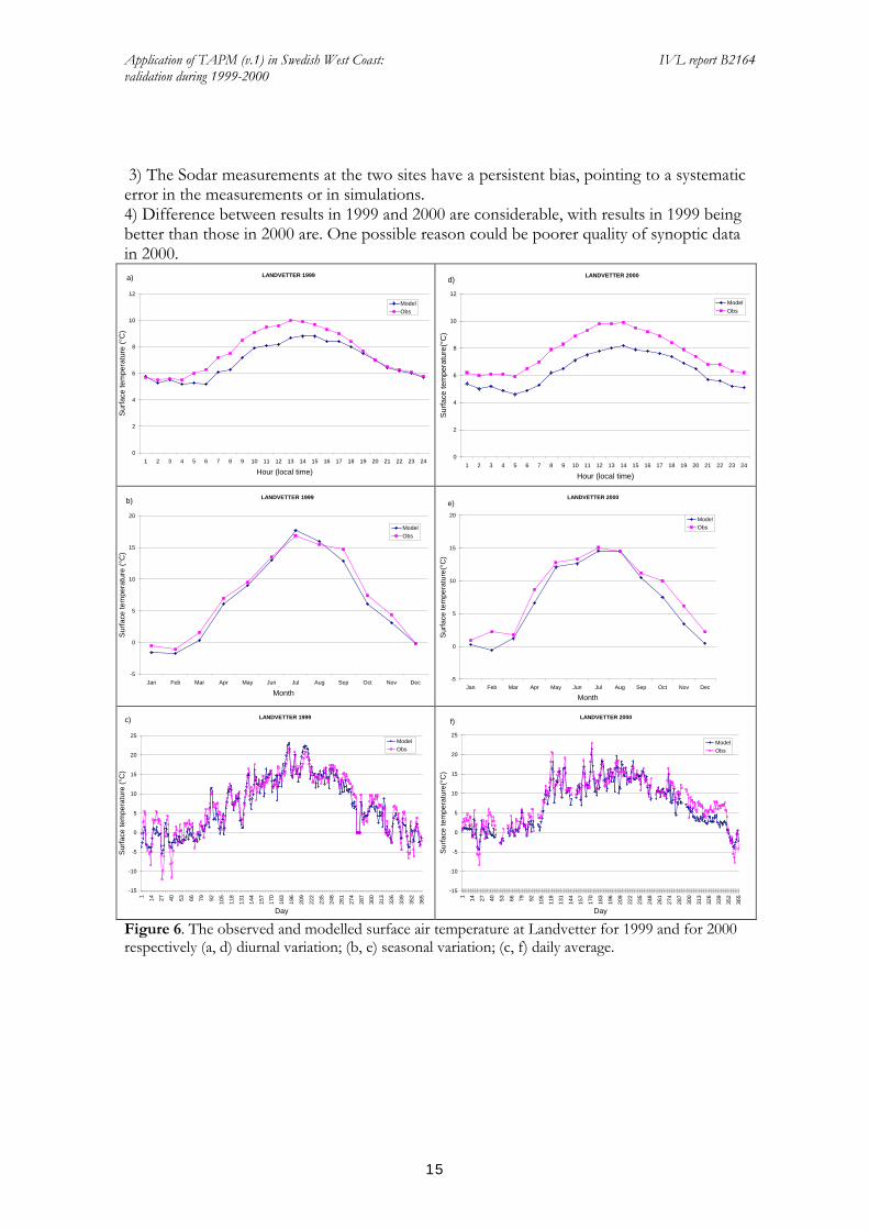
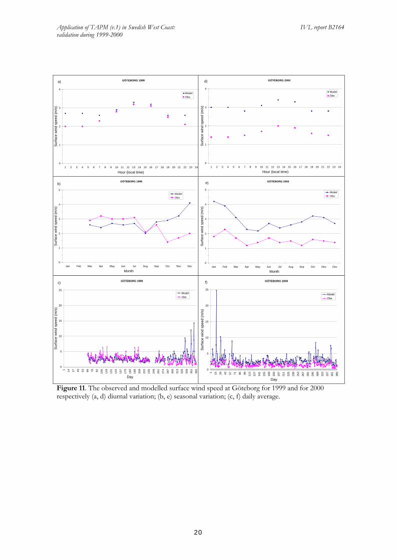
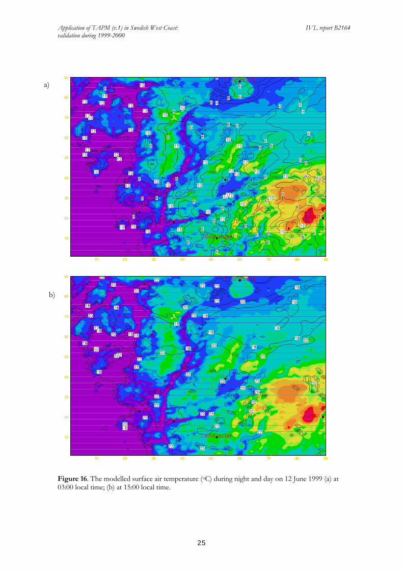
For surface temperature (Table 2b), high correlation (greater than 0.92) and small square error (0.03 to 0.05oC) were found between the model results and the measurements. In general, the model systematically underestimated surface temperature by about 1oC. The surface wind (Table 2a) was also well simulated, but the correlation coefficients were somewhat lower compared to those of temperature. The modelled horizontal wind was thus overestimated at urban site (Göteborg) and underestimated at non-urban sites (Landvetter as well as Säve) in 1999. There were considerable changes in the statistics between 1999 and 2000, indicating that year-to-year changes are important for this region. The diurnal variations, seasonal variations and daily averages of the observed and simulated surface temperature are presented in Figures 5-7 for 1999 and 2000 respectively. The slight underestimate of the surface temperature in Göteborg appears to be systematic with respect to time, as shown by Figures 5a and 5d. This is especially pronounced for 2000. However, the seasonal variations as shown by Figure 5e indicate that the underestimates mainly occur during cold months. This may be partly due to the neglect of the anthropogenic heating in the city. For Landvetter the underestimate mainly appears during the day (Figure 6a) even if the year-to-year change can be large (Figure 6a and Figure 6d). Once again, cold months have a larger underestimate than the warm months (Figure 6b and Figure 6e). Simulations for Säve (Figure 7) show a similar pattern as for Göteborg and Landvetter. The diurnal variations, seasonal variations and daily averages of the observed and simulated surface wind direction (Figures 8-10) and speed (Figures 11-13) are displayed for 1999 and 2000 respectively. In general, the simulations for wind direction follow the evolution of the observations well, although there are fairly systematic differences. For wind speed, the differences between 1999 and 2000 were fairly large especially for Göteborg (Figure 11d). The model has a strong ability to simulate urban heat island effect, which can be seen in Figure 14. The figure shows that the temperature difference between the urban (Göteborg) and the suburban (Landvetter and Säve) stations can reach 1.4-3.4 ºC (Göteborg-Landvetter) and 1.5-3.8 ºC) (Göteborg-Säve) on the hourly basis for modelled results and for measurements. The simulations follow the observations well, though the difference varies with year. A very important feature of TAPM is its ability to explicitly deal with surface energy budget and temperature, which allows simulation of thermally driven wind systems. An examination of the modelled results reveals that the model performs well in modeling mesoscale wind system, such as land-sea breeze circulation. As an example, Figures 15-18 display a simulation of such a wind system during 1999 in various ways. The figures show that during the daytime, solar radiation heats the ground faster than the sea, which results in higher air temperature over land compared to the sea. Therefore, air with lower density ascends over land and air with higher density descends over sea. Near the surface, air flow from the sea to the land, leading to development of sea breeze. During clear nights, the cooling of land is faster than the sea, hence air blow from land to sea over the surface, leading to formation of land breeze. The return flow of the sea breeze can be seen (Figure 17b) at the model level 9 (750 m).


14

4.2 Profile comparison

The statistics of observed and modelled wind profiles at selected levels at Hunneberg and Borås are listed in Table 3 and Table 4, respectively.

Figure 5. The observed and modelled surface air temperature at Göteborg for 1999 and for 2000 respectively (a, d) diurnal variation; (b, e) seasonal variation; (c, f) daily average. From the results following features are obvious: 1) The evolution of the simulated upper winds follows those of the observed fairly well, as reflected in the correlation coefficients that are comparable to those in the surface comparison. 2) The agreements at the two sites are comparable.

GÖTEBORG 1999

0

2

4

6

8

10

12

14

1 2 3 4 5 6 7 8 9 10 11 12 13 14 15 16 17 18 19 20 21 22 23 24

Hour (local time)

Sur

face

tem

pera

ture

(°C

)

ModelObs

a) GÖTEBORG 2000

0

2

4

6

8

10

12

14

1 2 3 4 5 6 7 8 9 10 11 12 13 14 15 16 17 18 19 20 21 22 23 24

Hour (local time)

Surfa

ce te

mpe

ratu

re (°

C)

ModelObs

d)

GÖTEBORG 1999

0

4

8

12

16

20

Jan Feb Mar Apr May Jun Jul Aug Sep Oct Nov Dec

Month

Surfa

ce te

mpe

ratu

re (°

C)

ModelObs

b)GÖTEBORG 2000

0

4

8

12

16

20


Month

Surfa

ce te

mpe

ratu

re (°

C)

ModelObs

e)

GÖTEBORG 1999

-10

-5

0

5

10

15

20

25

30

1 14 27 40 53 66 79 92 105

118

131

144

157

170

183

196

209

222

235

248

261

274

287

300

313

326

339

352

365

Day

Surfa

ce te

mpe

ratu

re(°

C)

ModelObs

c)GÖTEBORG 2000

-10

-5

0

5

10

15

20

25

30

1 14 27 40 53 66 79 92 105

118

131

144

157

170

183

196

209

222

235

248

261

274

287

300

313

326

339

352

365

Day

Surfa

ce te

mpe

ratu

re (°

C)

ModelObs

f)


15

3) The Sodar measurements at the two sites have a persistent bias, pointing to a systematic error in the measurements or in simulations. 4) Difference between results in 1999 and 2000 are considerable, with results in 1999 being better than those in 2000 are. One possible reason could be poorer quality of synoptic data in 2000.

Figure 6. The observed and modelled surface air temperature at Landvetter for 1999 and for 2000 respectively (a, d) diurnal variation; (b, e) seasonal variation; (c, f) daily average.

LANDVETTER 1999

0

2

4

6

8

10

12

1 2 3 4 5 6 7 8 9 10 11 12 13 14 15 16 17 18 19 20 21 22 23 24

Hour (local time)

Surfa

ce te

mpe

ratu

re (°

C)

ModelObs

a) LANDVETTER 2000

0

2

4

6

8

10

12

1 2 3 4 5 6 7 8 9 10 11 12 13 14 15 16 17 18 19 20 21 22 23 24

Hour (local time)

Surfa

ce te

mpe

ratu

re(°

C)

ModelObs

d)

LANDVETTER 1999

-5

0

5

10

15

20


Month

Surfa

ce te

mpe

ratu

re (°

C)

ModelObs

b) LANDVETTER 2000

-5

0

5

10

15

20


Month

Surfa

ce te

mpe

ratu

re(°

C)

ModelObs

e)

LANDVETTER 1999

-15

-10

-5

0

5

10

15

20

25

1 14 27 40 53 66 79 92 105

118

131

144

157

170

183

196

209

222

235

248

261

274

287

300

313

326

339

352

365

Day

Surfa

ce te

mpe

ratu

re (°

C)

Model Obs

c) LANDVETTER 2000

-15

-10

-5

0

5

10

15

20

25

1 14 27 40 53 66 79 92 105

118

131

144

157

170

183

196

209

222

235

248

261

274

287

300

313

326

339

352

365

Day

Surfa

ce te

mpe

ratu

re(°

C)

ModelObs

f)


16

Figure 7. The observed and modelled surface air temperature at Säve for 1999 and for 2000 respectively (a, d) diurnal variation; (b, e) seasonal variation; (c, f) daily average.

SÄVE 1999

0

2

4

6

8

10

12

1 2 3 4 5 6 7 8 9 10 11 12 13 14 15 16 17 18 19 20 21 22 23 24

Hour (local time)

Surfa

ce te

mpe

ratu

re (°

C)

ModelObs

a) SÄVE 2000

0

2

4

6

8

10

12

1 2 3 4 5 6 7 8 9 10 11 12 13 14 15 16 17 18 19 20 21 22 23 24

Hour (local time)

Surfa

ce te

mpe

ratu

re (°

C)

ModelObs

d)

SÄVE 1999

-5

0

5

10

15

20


Month

Surfa

ce te

mpe

ratu

re (°

C)

ModelObs

b) SÄVE 2000

-5

0

5

10

15

20


Month

Surfa

ce te

mpe

ratu

re (°

C)

ModelObs

e)

SÄVE 1999

-15

-10

-5

0

5

10

15

20

25

30

1 14 27 40 53 66 79 92 105

118

131

144

157

170

183

196

209

222

235

248

261

274

287

300

313

326

339

352

365

Day

Sur

face

tem

pera

ture

(°C

)

ModelObs

c) SÄVE 2000

-15

-10

-5

0

5

10

15

20

25

30

1 14 27 40 53 66 79 92 105

118

131

144

157

170

183

196

209

222

235

248

261

274

287

300

313

326

339

352

365

Day

Surfa

ce te

mpe

ratu

re (°

C)

ModelObs

f)


17

Figure 8. The observed and modelled surface wind direction at Göteborg for 1999 and for 2000 respectively (a, d) diurnal variation; (b, e) seasonal variation; (c, f) daily average.

GÖTEBORG 1999

90

135

180

225

270

1 2 3 4 5 6 7 8 9 10 11 12 13 14 15 16 17 18 19 20 21 22 23 24

Hour (local time)

Sur

face

win

d di

rect

ion

(º)

ModelObs

a) GÖTEBORG 2000

90

135

180

225

270

1 2 3 4 5 6 7 8 9 10 11 12 13 14 15 16 17 18 19 20 21 22 23 24

Hour (local time)

Sur

face

win

d di

rect

ion

(º)

ModelObs

d)

GÖTEBORG 1999

90

135

180

225

270


Month

Sur

face

win

d di

rect

ion

(º)

ModelObs

b) GÖTEBORG 2000

90

135

180

225

270


Month

Sur

face

win

d di

rect

ion

(º)

ModelObs

e)

GÖTEBORG 1999

0

90

180

270

360

1 14 27 40 53 66 79 92 105

118

131

144

157

170

183

196

209

222

235

248

261

274

287

300

313

326

339

352

365

Day

Sur

face

win

d di

rect

ion

(º)

ModelObs

c) GÖTEBORG 2000

0

90

180

270

360

1 14 27 40 53 66 79 92 105

118

131

144

157

170

183

196

209

222

235

248

261

274

287

300

313

326

339

352

365

Day

Sur

face

win

d di

rect

ion

(º)

ModelObs

f)


18

Figure 9. The observed and modelled surface wind direction at Landvetter for 1999 and for 2000 respectively (a, d) diurnal variation; (b, e) seasonal variation; (c, f) daily average.

LANDVETTER 1999

90

135

180

225

270

1 2 3 4 5 6 7 8 9 10 11 12 13 14 15 16 17 18 19 20 21 22 23 24

Hour (local time)

Sur

face

win

d di

rect

ion

(º)

ModelObs

a) LANDVETTER 2000

90

135

180

225

270

1 2 3 4 5 6 7 8 9 10 11 12 13 14 15 16 17 18 19 20 21 22 23 24

Hour (local time)

Sur

face

win

d di

rect

ion

(º)

ModelObs

d)

LANDVETTER 1999

90

135

180

225

270


Month

Sur

face

win

d di

rect

ion

(º)

ModelObs

b) LANDVETTER 2000

90

135

180

225

270


Month

Sur

face

win

d di

rect

ion

(º)

ModelObs

e)

LANDVETTER 1999

0

90

180

270

360

1 14 27 40 53 66 79 92 105

118

131

144

157

170

183

196

209

222

235

248

261

274

287

300

313

326

339

352

365

Day

Sur

face

win

d di

rect

ion

(º)

Model Obs

c) LANDVETTER 2000

0

90

180

270

360

1 15 29 43 57 71 85 99 113

127

141

155

169

183

197

211

225

239

253

267

281

295

309

323

337

351

365

Day

Surfa

ce w

ind

dire

ctio

n (º)

ModelObs

f)


19

Figure 10. The observed and modelled surface wind direction at Säve for 1999 and for 2000 respectively (a, d) diurnal variation; (b, e) seasonal variation; (c, f) daily average.

SÄVE 1999

90

135

180

225

270

1 2 3 4 5 6 7 8 9 10 11 12 13 14 15 16 17 18 19 20 21 22 23 24

Hour (local time)

Sur

face

win

d di

rect

ion

(º)

ModelObs

a) SÄVE 2000

90

135

180

225

270

1 2 3 4 5 6 7 8 9 10 11 12 13 14 15 16 17 18 19 20 21 22 23 24

Hour (local time)

Surfa

ce w

ind

dire

ctio

n (º

)

ModelObs

d)

SÄVE 1999

90

135

180

225

270


Month

Sur

face

win

d di

rect

ion

(º)

ModelObs

b) SÄVE 2000

90

135

180

225

270


Month

Sur

face

win

d di

rect

ion

(º)

ModelObs

e)

SÄVE 1999

0

90

180

270

360

1 14 27 40 53 66 79 92 105

118

131

144

157

170

183

196

209

222

235

248

261

274

287

300

313

326

339

352

365

Day

Sur

face

win

d di

rect

ion

(º)

ModelObs

c) SÄVE 2000

0

90

180

270

360

1 14 27 40 53 66 79 92 105

118

131

144

157

170

183

196

209

222

235

248

261

274

287

300

313

326

339

352

365

Day

Sur

face

win

d di

rect

ion

(º)

ModelObs

f)


20

Figure 11. The observed and modelled surface wind speed at Göteborg for 1999 and for 2000 respectively (a, d) diurnal variation; (b, e) seasonal variation; (c, f) daily average.

GÖTEBORG 1999

0

1

2

3

4

1 2 3 4 5 6 7 8 9 10 11 12 13 14 15 16 17 18 19 20 21 22 23 24

Hour (local time)

Sur

face

win

d sp

eed

(m/s

)

ModelObs

a) GÖTEBORG 2000

0

1

2

3

4

1 2 3 4 5 6 7 8 9 10 11 12 13 14 15 16 17 18 19 20 21 22 23 24

Hour (local time)

Sur

face

win

d sp

eed

(m/s

)

ModelObs

d)

GÖTEBORG 1999

0

1

2

3

4

5


Month

Sur

face

win

d sp

eed

(m/s

)

ModelObs

b)GÖTEBORG 2000

0

1

2

3

4

5


Month

Sur

face

win

d sp

eed

(m/s

)

ModelObs

e)

GÖTEBORG 1999

0

5

10

15

20

25

1 14 27 40 53 66 79 92 105

118

131

144

157

170

183

196

209

222

235

248

261

274

287

300

313

326

339

352

365

Day

Sur

face

win

d sp

eed

(m/s

)

ModelObs

c) GÖTEBORG 2000

0

5

10

15

20

25

1 15 29 43 57 71 85 99 113

127

141

155

169

183

197

211

225

239

253

267

281

295

309

323

337

351

365

Day

Surfa

ce w

ind

spee

d (m

/s)

ModelObs

f)


21

Figure 12. The observed and modelled surface wind speed at Landvetter for 1999 and for 2000 respectively (a, d) diurnal variation; (b, e) seasonal variation; (c, f) daily average.

LANDVETTER 1999

0

1

2

3

4

5

6

1 2 3 4 5 6 7 8 9 10 11 12 13 14 15 16 17 18 19 20 21 22 23 24

Hour (local time)

Sur

face

win

d sp

eed

(m/s

)

ModelObs

a) LANDVETTER 2000

0

1

2

3

4

5

6

1 2 3 4 5 6 7 8 9 10 11 12 13 14 15 16 17 18 19 20 21 22 23 24

Hour (local time)

Surfa

ce w

ind

spee

d (m

/s)

ModelObs

d)

LANDVETTER 1999

0

1

2

3

4

5

6

7

8


Month

Sur

face

win

d sp

eed

(m/s

)

ModelObs

b)LANDVETTER 2000

0

1

2

3

4

5

6

7

8


Month

Sur

face

win

d sp

eed

(m/s

)

ModelObs

e)

LANDVETTER 1999

0

5

10

15

20

25

30

1 14 27 40 53 66 79 92 105

118

131

144

157

170

183

196

209

222

235

248

261

274

287

300

313

326

339

352

365

Day

Sur

face

win

d sp

eed

(m/s

)

Model Obs

c) LANDVETTER 2000

0

5

10

15

20

25

30

1 14 27 40 53 66 79 92 105

118

131

144

157

170

183

196

209

222

235

248

261

274

287

300

313

326

339

352

365

Day

Sur

face

win

d sp

eed

(m/s

)

ModelObs

f)


22

Figure 13. The observed and modelled surface wind speed at Säve for 1999 and for 2000 respectively (a, d) diurnal variation; (b, e) seasonal variation; (c, f) daily average.

SÄVE 1999

0

1

2

3

4

5

6

1 2 3 4 5 6 7 8 9 10 11 12 13 14 15 16 17 18 19 20 21 22 23 24

Hour (local time)

Sur

face

win

d sp

eed

(m/s

)

ModelObs

a) SÄVE 2000

0

1

2

3

4

5

6

1 2 3 4 5 6 7 8 9 10 11 12 13 14 15 16 17 18 19 20 21 22 23 24

Hour (local time)

Sur

face

win

d sp

eed

(m/s

)

ModelObs

d)

SÄVE 1999

0

1

2

3

4

5

6

7


Month

Sur

face

win

d sp

eed

(m/s

)

ModelObs

b) SÄVE 2000

0

1

2

3

4

5

6

7


Month

Sur

face

win

d sp

eed

(m/s

)

ModelObs

e)

SÄVE 1999

0

5

10

15

20

25

30

1 14 27 40 53 66 79 92 105

118

131

144

157

170

183

196

209

222

235

248

261

274

287

300

313

326

339

352

365

Day

Sur

face

win

d sp

eed

(m/s

)

ModelObs

c)SÄVE 2000

0

5

10

15

20

25

30

1 14 27 40 53 66 79 92 105

118

131

144

157

170

183

196

209

222

235

248

261

274

287

300

313

326

339

352

365

Day

Sur

face

win

d sp

eed

(m/s

)

ModelObs

f)


23

Figure 14. The observed and modelled surface temperature difference between Göteborg and Landvetter (G-L), as well as between Göteborg and Säve (G-S) for 1999 and for 2000 respectively (a, d) diurnal variation; (b, e) seasonal variation; (c, f) daily average.

0

1

2

3

4

1 2 3 4 5 6 7 8 9 10 11 12 13 14 15 16 17 18 19 20 21 22 23 24

Hour (local time)

Sur

face

tem

pera

ture

diff

eren

ce (°

C)

G-L(Model)G-S(Model)G-L(Obs)G-S(Obs)

a)

0

1

2

3

4

1 2 3 4 5 6 7 8 9 10 11 12 13 14 15 16 17 18 19 20 21 22 23 24

Hour (local time)

Sur

face

tem

pera

ture

diff

eren

ce (°

C)


d)

-1

-0,5

0

0,5

1

1,5

2


Month

Sur

face

tem

pera

ture

diff

eren

ce (°

C)


b)

-3

-2

-1

0

1

2

3

4

5

1 14 27 40 53 66 79 92 105

118

131

144

157

170

183

196

209

222

235

248

261

274

287

300

313

326

339

352

365

Day

Sur

face

tem

pera

ture

diff

eren

ce (°

C)


c)

-3

-2

-1

0

1

2

3

4

5

1 14 27 40 53 66 79 92 105

118

131

144

157

170

183

196

209

222

235

248

261

274

287

300

313

326

339

352

365

Day

Sur

face

tem

pera

ture

diff

eren

ce (°

C)


f)


24

Figure 15. The modelled surface wind during night and day on 12 June 1999 a) at 03:00 local time; b) at 15:00 local time.

a)

b)


25

Figure 16. The modelled surface air temperature (oC) during night and day on 12 June 1999 (a) at 03:00 local time; (b) at 15:00 local time.

a)

b)


26

Figure 17. The modelled cross section (X-Z or u-10w) of wind during night and day on 12 June 1999 a) at 03:00 local time; b) at 15:00 local time. Unit of u and w m/s.

a)

b)


27

Figure 18. The modelled mixing height (m) during night and day on 12 June 1999 a) at 03:00 local time; b) at 15:00 local time. Table 3a. Comparison between the modelled and observed wind profiles at Hunneberg in 1999. Unit of wind speed: m/s.

a)

b)


28

Component

Height Correlation coefficient

Modelled average

Observed average

Bias RMSE

wind-u 50m (7672*) 0.78 0.2 wind-v 0.66 0.2 wind speed 0.54 6.0 3.5 2.5 0.2 wind-u 100m (7674*) 0.81 0.2 wind-v 0.70 0.2 wind speed 0.60 7.0 5.5 1.5 0.3 wind-u 150m (7658*) 0.82 0.2 wind-v 0.70 0.2 wind speed 0.62 7.8 6.6 1.2 0.3 wind-u 200m (7015*) 0.81 0.2 wind-v 0.70 0.2 wind speed 0.57 8.5 7.2 1.3 0.3 wind-u 300m (3908*) 0.76 0.3 wind-v 0.69 0.3 wind speed 0.50 9.5 7.8 1.7 0.4 wind-u 400m (1253*) 0.73 0.4 wind-v 0.68 0.4 wind speed 0.51 10.5 8.2 2.3 0.5 * sample number for statistics Table 3b. Comparison between the modelled and observed wind profiles at Hunneberg in 2000. Unit of wind speed: m/s. Component Height Correlation

coefficient Modelle

d average

Observedaverage

Bias RMSE

wind-u 50m (100*) -0.46 0.9 wind-v 0.57 0.6 wind speed 0.39 5.4 4.1 1.3 0.9 wind-u 100m (5603*) 0.65 0.3 wind-v 0.42 0.3 wind speed 0.47 8.2 4.7 3.5 0.3 wind-u 150m (5601*) 0.64 0.3 wind-v 0.44 0.3 wind speed 0.51 9.0 6.5 2.5 0.3 wind-u 200m (5571*) 0.62 0.3 wind-v 0.48 0.3 wind speed 0.50 9.7 7.4 2.3 0.4

wind-u 300m (4681*) 0.53 0.3 wind-v 0.52 0.3 wind speed 0.45 10.6 8.2 2.4 0.4 wind-u 400m (2923*) 0.37 0.4 wind-v 0.45 0.4 wind speed 0.22 11.2 8.4 2.8 0.5 * sample number for statistics


29

Table 4a. Comparison between the modelled and observed wind profiles at Borås in 1999. Unit of wind speed: m/s. Component Height Correlation


Observed average

Bias RMSE

Wind-u 50m (7297*) 0.80 0.2 Wind-v 0.71 0.2 Wind speed 0.60 5.3 3.8 1.5 0.2 Wind-u 100m (7851) 0.83 0.2 Wind-v 0.72 0.2 Wind speed 0.64 6.6 5.0 1.6 0.2 wind-u 150m (7364*) 0.77 0.2 wind-v 0.71 0.2 wind speed 0.49 7.5 5.5 2.0 0.3 wind-u 200m (5013*) 0.77 0.3 wind-v 0.71 0.2 wind speed 0.51 8.0 6.1 1.9 0.3 wind-u 300m (1544*) 0.81 0.4 wind-v 0.67 0.4 wind speed 0.45 9.8 8.0 1.8 0.4 wind-u 400m (298*) 0.87 0.5 wind-v 0.70 0.5 wind speed 0.56 11.7 9.6 2.1 0.6 * sample number for statistics Table 4b. Comparison between the modelled and observed wind profiles at Borås in 2000. Unit of wind speed: m/s. Component Height Correlation


Observed average

Bias RMSE

wind-u 50m (4773*) -0.07 0.2 wind-v -0.06 0.2

wind speed 0.01 6.2 2.5 3.7 0.3 wind-u 100m (7113*) 0.69 0.2 wind-v 0.53 0.2

Wind speed 0.47 7.7 4.2 3.5 0.3 wind-u 150m (7020*) 0.67 0.2 wind-v 0.57 0.3




Wind speed 0.12 11.4 9.0 2.4 0.8 * sample number for statistics


30

5. Model outputs The output of TAPM is rich, covering both 2D and 3D fields. The 2D fields are:

• total solar radiation, net radiation, sensible heat flux, evaporative heat flux, friction velocity, potential virtual temperature, potential temperature, convective velocity, mixing height, screen-level temperature, screen-level relative humidity, surface temperature and rainfall,

The 3D fields are:

• horizontal wind speed, horizontal wind direction, vertical velocity, temperature, relative humidity, and potential temperature and turbulence kinetic energy.

As examples, Figure 18 gives a snapshot of modelled mixing height during one day and one night. The figure shows distinct diurnal variations in mixing height, which is strong at the day time due to the unstable atmosphere and weak at the nigh time due to the stable stratification of the atmosphere.

6. Comments on use of TAPM

6.1. Computer requirements

A fast PC is required since the computer run time for TAPM is relatively long. However, the run-time will vary depending on your choice of model configurations.

6.2 Model limitations

Although TAPM performs well in many aspects, it has some major limitations as the following: (1) TAPM should not be used for larger domains than 1000 km by 1000 km, due to curvature of the earth. (2) The GRS photochemistry option in the model may not be suitable for examining small perturbations in emissions inventories, particularly in VOC emissions, due to the highly lumped approach taken for VOC's in this mechanism. VOC reactivates should also be chosen carefully for each region of application.

6.3. Soil moisture setting

The soil moisture is an import parameter in determining the surface energy balance. Based on our experience, a seasonal variable should be used. The following soil moisture (Table 5) is recommended for the model running for the Swedish West Coast. This table is based


31

on NCEP reanalysis of 1999 over the area. Further study may be needed to specify it in a better way.

Table 5. Deep soil volumetric moisture in content m3 m-3 (i.e. the volume of water per volume of soil) used in model run

Mon Jan Feb Mar Apr May Jun Jul Aug Sep Oct Nov Dec

Value 0.29 0.30 0.28 0.24 0.21 0.19 0.18 0.19 0.21 0.23 0.26 0.28

6.4. Output processing

Two extra programs (tapm2outa.exe and glc2glca.exe) can be used to transform the TAPM binary outputs into ASCII format, which can be seen in Appendix in detail. Another two programs, named readmet.exe and readcon.exe, have been designed to convert ASCII format files into binary format for Grads uses. For further information see Appendix 2. The output of TAPM can also be presented based on Grads system using *.gs files.

7. Conclusions Based on the comparisons between the TAPM output from the two years run and the surface/profile measurements on air temperature and wind, it has been found that TAPM performs well in simulating air temperature and wind for Swedish conditions. These parameters are the two most important fields to drive the air pollution modelling. In addition, TAPM has strong ability in modelling sea-land breeze and urban heat island effect. As such, it is concluded that in the future TAPM can be applied in meteorological modelling and environmental impact assessment in Sweden with confidence.

Acknowledgement Support to this study was partly founded by the Swedish Environmental Protection Agency (802-470-00-7) and the Swedish Road Administration. We would also like to acknowledge Leif Enger and David Svenson (Luft i Väst) for letting us use their SODAR data. We would also like to thank Karin Sjöberg for her comments on the manuscript.

Reference Hurley, P.J. (1999a). ‘The Air Pollution Model (TAPM) Version 1: Technical Description

and Examples’, CAR Technical Paper No. 43. 42 p.

Hurley, P.J. (1999b). ’The air pollution model (TAPM) version 1: User manual’. Internal paper 12 of CSIRO Atmospheric Research Division 22 p.


32

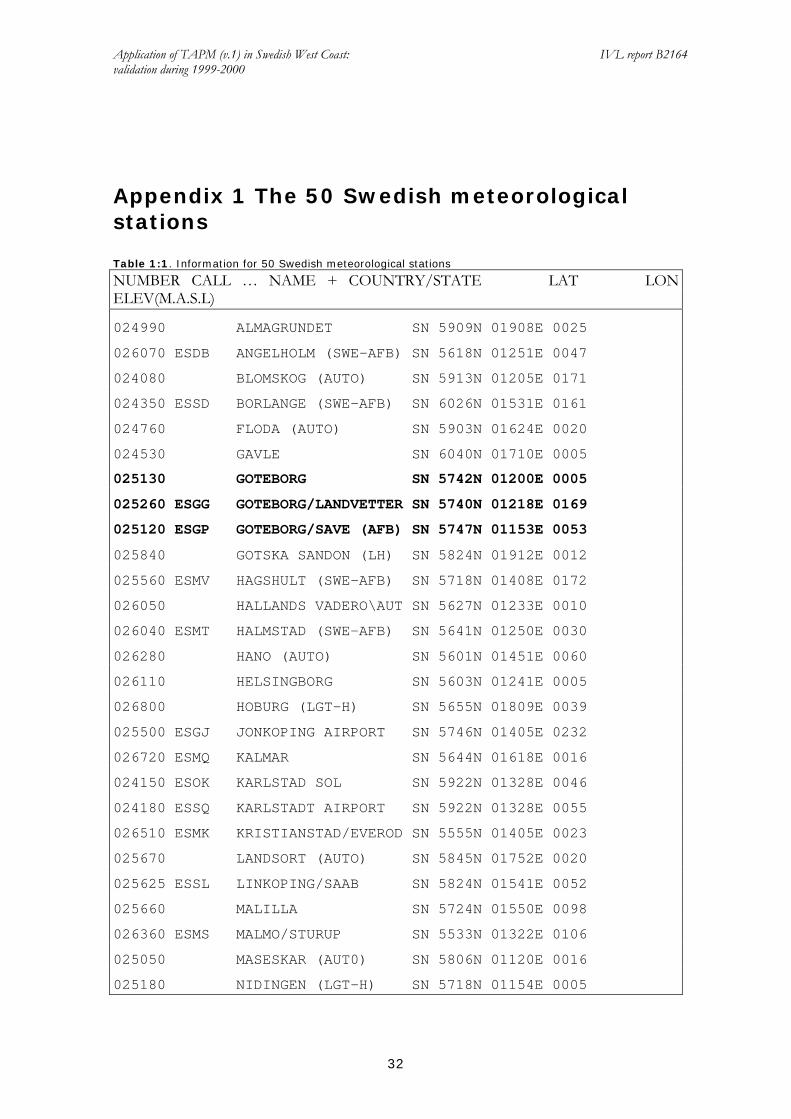
Appendix 1 The 50 Swedish meteorological stations

Table 1:1. Information for 50 Swedish meteorological stations NUMBER CALL … NAME + COUNTRY/STATE LAT LON ELEV(M.A.S.L)

024990 ALMAGRUNDET SN 5909N 01908E 0025

026070 ESDB ANGELHOLM (SWE-AFB) SN 5618N 01251E 0047

024080 BLOMSKOG (AUTO) SN 5913N 01205E 0171

024350 ESSD BORLANGE (SWE-AFB) SN 6026N 01531E 0161

024760 FLODA (AUTO) SN 5903N 01624E 0020

024530 GAVLE SN 6040N 01710E 0005

025130 GOTEBORG SN 5742N 01200E 0005

025260 ESGG GOTEBORG/LANDVETTER SN 5740N 01218E 0169

025120 ESGP GOTEBORG/SAVE (AFB) SN 5747N 01153E 0053

025840 GOTSKA SANDON (LH) SN 5824N 01912E 0012

025560 ESMV HAGSHULT (SWE-AFB) SN 5718N 01408E 0172

026050 HALLANDS VADERO\AUT SN 5627N 01233E 0010

026040 ESMT HALMSTAD (SWE-AFB) SN 5641N 01250E 0030

026280 HANO (AUTO) SN 5601N 01451E 0060

026110 HELSINGBORG SN 5603N 01241E 0005

026800 HOBURG (LGT-H) SN 5655N 01809E 0039

025500 ESGJ JONKOPING AIRPORT SN 5746N 01405E 0232

026720 ESMQ KALMAR SN 5644N 01618E 0016

024150 ESOK KARLSTAD SOL SN 5922N 01328E 0046

024180 ESSQ KARLSTADT AIRPORT SN 5922N 01328E 0055

026510 ESMK KRISTIANSTAD/EVEROD SN 5555N 01405E 0023

025670 LANDSORT (AUTO) SN 5845N 01752E 0020

025625 ESSL LINKOPING/SAAB SN 5824N 01541E 0052

025660 MALILLA SN 5724N 01550E 0098

026360 ESMS MALMO/STURUP SN 5533N 01322E 0106

025050 MASESKAR (AUT0) SN 5806N 01120E 0016

025180 NIDINGEN (LGT-H) SN 5718N 01154E 0005


33

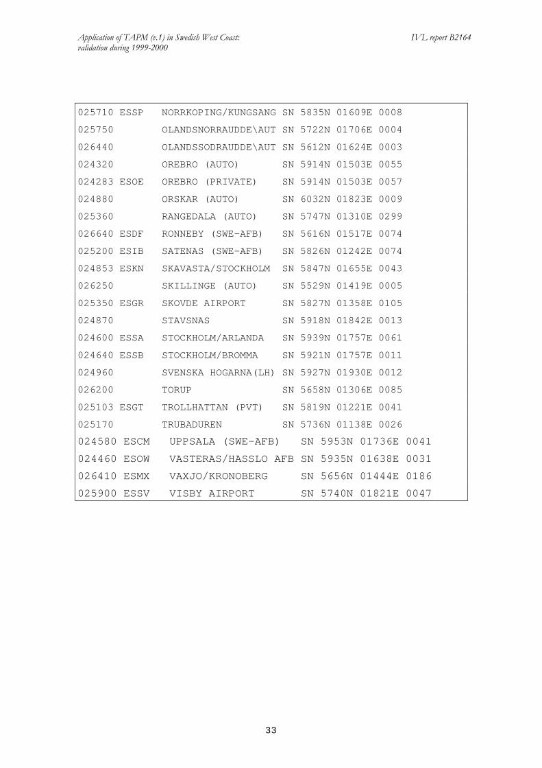
025710 ESSP NORRKOPING/KUNGSANG SN 5835N 01609E 0008

025750 OLANDSNORRAUDDE\AUT SN 5722N 01706E 0004

026440 OLANDSSODRAUDDE\AUT SN 5612N 01624E 0003

024320 OREBRO (AUTO) SN 5914N 01503E 0055

024283 ESOE OREBRO (PRIVATE) SN 5914N 01503E 0057

024880 ORSKAR (AUTO) SN 6032N 01823E 0009

025360 RANGEDALA (AUTO) SN 5747N 01310E 0299

026640 ESDF RONNEBY (SWE-AFB) SN 5616N 01517E 0074

025200 ESIB SATENAS (SWE-AFB) SN 5826N 01242E 0074

024853 ESKN SKAVASTA/STOCKHOLM SN 5847N 01655E 0043

026250 SKILLINGE (AUTO) SN 5529N 01419E 0005

025350 ESGR SKOVDE AIRPORT SN 5827N 01358E 0105

024870 STAVSNAS SN 5918N 01842E 0013

024600 ESSA STOCKHOLM/ARLANDA SN 5939N 01757E 0061

024640 ESSB STOCKHOLM/BROMMA SN 5921N 01757E 0011

024960 SVENSKA HOGARNA(LH) SN 5927N 01930E 0012

026200 TORUP SN 5658N 01306E 0085

025103 ESGT TROLLHATTAN (PVT) SN 5819N 01221E 0041

025170 TRUBADUREN SN 5736N 01138E 0026

024580 ESCM UPPSALA (SWE-AFB) SN 5953N 01736E 0041

024460 ESOW VASTERAS/HASSLO AFB SN 5935N 01638E 0031

026410 ESMX VAXJO/KRONOBERG SN 5656N 01444E 0186

025900 ESSV VISBY AIRPORT SN 5740N 01821E 0047


34

Appendix 2 Tools developed 1. tapm2outa.exe It converts TAPM meteorological output *.out and *.rfl files to an ASCII *.outa file. For all or a subset of specified dates can be run using the following command: echo sdate edate t100a | tapm2outa.exe where, sdate is the start date (yyyymmdd) that you want in the *.outa file, edate is the end date (yyyymmdd) that you want in the *.outa file,

t100a is the filename prefix for the *.out file (e.g. t100a.out) and produces a *.outa file (e.g. t100a.outa). The file format for the *.outa file is as follows:

• fixed format with READ1 using format 10i8 (10 integers per line with each integer using 8 characters)

• fixed format with READ2 using format 10f8.2 (10 floating point numbers per line with each number using 8 characters with 2 digits after the decimal point)

READ1: nx, ny, nz, dx, dy READ2: ((zs(i,j),i=1,nx),j=1,ny) READ2: (((z(i,j,k),i=1,nx),j=1,ny),k=1,nz) Repeated for each simulation hour: READ1: date, hour READ2: ((tsr(i,j),i=1,nx),j=1,ny) READ2: ((net(i,j),i=1,nx),j=1,ny) READ2: ((sens(i,j),i=1,nx),j=1,ny) READ2: ((evap(i,j),i=1,nx),j=1,ny) READ2: ((ustar(i,j),i=1,nx),j=1,ny) READ2: ((pvstar(i,j),i=1,nx),j=1,ny) READ2: ((ptstar(i,j),i=1,nx),j=1,ny) READ2: ((wstar(i,j),i=1,nx),j=1,ny) READ2: ((zmix(i,j),i=1,nx),j=1,ny) READ2: ((tscr(i,j),i=1,nx),j=1,ny) READ2: ((rhscr(i,j),i=1,nx),j=1,ny) READ2: ((tsurf(i,j),i=1,nx),j=1,ny) READ2: ((rain(i,j),i=1,nx),j=1,ny) READ2: (((ws(i,j),i=1,nx),j=1,ny),k=1,nz) READ2: (((wd(i,j),i=1,nx),j=1,ny),k=1,nz) READ2: (((ww(i,j),i=1,nx),j=1,ny),k=1,nz) READ2: (((tt(i,j),i=1,nx),j=1,ny),k=1,nz) READ2: (((rh(i,j),i=1,nx),j=1,ny),k=1,nz) READ2: (((pt(i,j),i=1,nx),j=1,ny),k=1,nz) READ2: (((tke(i,j),i=1,nx),j=1,ny),k=1,nz) with variables: nx number of west-east (x) grid points for the meteorological grid, ny number of south-north (y) grid points for the meteorological grid, nz number of vertical (z) grid points (levels) for the meteorological grid, dx west-east (x) grid spacing (m) for the meteorological grid, dy south-north (y) grid spacing (m) for the meteorological grid, zs smoothed terrain height (m), z height above the terrain (m), date date (yyyymmdd), hour hour of simulation (1-24), tsr total solar radiation (W m-2), net net radiation (W m-2), sens sensible heat flux (W m-2), evap evaporative heat flux (W m-2), ustar friction velocity scale (m s-1), pvstar potential virtual temperature scale (K), ptstar potential temperature scale (K),


35

wstar convective velocity scale (m s-1), zmix mixing height (m), tscr screen-level temperature (K), rhsrc screen-level relative humidity (%), tsurf surface temperature (K), rain rainfall (mm hr-1), ws horizontal wind speed (m s-1), wd horizontal wind direction (o) (usual meteorological definition), ww vertical velocity (m s-1), tt temperature (K), rh relative humidity (%), pt potential temperature (K), tke turbulence kinetic energy (m2 s-2). Note that the meteorological grid (array) is oriented so that: grid( 1, 1, 1) is the south-west corner at the surface, grid(nx, 1, 1) is the south-east corner at the surface, grid( 1,ny, 1) is the north-west corner at the surface, grid(nx,ny, 1) is the north-east corner at the surface, and similarly for array index k = nz at the top of the grid.

2. glc2glca.exe It converts a TAPM concentration output *.glc file to an ASCII *.glca file and can be run

using the following command: echo t100atr1 | glc2glca.exe where, t100atr1 is the filename prefix for the *.glc file (e.g. t100atr1.glc) and produces a *.glca file (e.g. t100atr1.glca).The file format for *.glca files is as follows (space delimited free format): READ: nx, ny Repeated for each simulation hour: READ: idate, itime READ: ((ic(i,j),i=1,nx),j=1,ny) with variables: nx number of west-east (x) grid points for the concentration grid, ny number of south-north (y) grid points for the concentration grid, idate date (yyyymmdd), itime hour of simulation, ic concentration grid (array). Note that the array is oriented so that ic( 1, 1) is the south-west corner, ic(nx, 1) is the south-east corner, ic(1 ,ny) is the north-west corner, ic(nx,ny) is the north-east corner.

3. readmet.exe It converts TAPM meteorology output ASCII file (such as t10a.outa) to bin format files and can be run using the following command: echo sdate fname | readmet.exe where, sdate is starting date(6 characters, yymmdd) and fname is the file name of ASCII file(4 characters, for example, t10a).

4. readcon.exe It converts TAPM concentration output ASCII file to binary format file and can be run using the following command: echo fname | readcon.exe

where, fname is the file name of ASCII file(7 characters, for example, t10atr1)

5. *.gs

All *.gs files are used to present the TAPM outputs based on Grads system.

Documents

Application of TAPM (v.1) in Swedish West Coast ... . Deliang Chen. 1, 2, Tijian Wang. 1, 2, Marie Haeger-Eugensson. 1, Christine Achberger. 2, Katarina Borne. 2 . 1. IVL Swedish Environmental