Embed Size (px)
Citation preview

Artif Intell Rev (2015) 43:381–416DOI 10.1007/s10462-012-9383-6
Application of reinforcement learning to routingin distributed wireless networks: a review
Hasan A. A. Al-Rawi · Ming Ann Ng ·Kok-Lim Alvin Yau
Published online: 8 January 2013© Springer Science+Business Media Dordrecht 2013
Abstract The dynamicity of distributed wireless networks caused by node mobility,dynamic network topology, and others has been a major challenge to routing in such networks.In the traditional routing schemes, routing decisions of a wireless node may solely dependon a predefined set of routing policies, which may only be suitable for a certain networkcircumstances. Reinforcement Learning (RL) has been shown to address this routing chal-lenge by enabling wireless nodes to observe and gather information from their dynamic localoperating environment, learn, and make efficient routing decisions on the fly. In this article,we focus on the application of the traditional, as well as the enhanced, RL models, to routingin wireless networks. The routing challenges associated with different types of distributedwireless networks, and the advantages brought about by the application of RL to routingare identified. In general, three types of RL models have been applied to routing schemes inorder to improve network performance, namely Q-routing, multi-agent reinforcement learn-ing, and partially observable Markov decision process. We provide an extensive review onnew features in RL-based routing, and how various routing challenges and problems havebeen approached using RL. We also present a real hardware implementation of a RL-basedrouting scheme. Subsequently, we present performance enhancements achieved by the RL-based routing schemes. Finally, we discuss various open issues related to RL-based routingschemes in distributed wireless networks, which help to explore new research directions inthis area. Discussions in this article are presented in a tutorial manner in order to establish afoundation for further research in this field.
Keywords Q-routing · Routing ·Wireless networks · Q-learning · Reinforcement learning
H. A. A. Al-Rawi (B)·M. A. Ng · K.-L. A. YauDepartment of Computer Science and Networked System,Faculty of Science and Technology, Sunway University, No. 5 Jalan Universiti,Bandar Sunway, 46150 Petaling Jaya, Selangor, Malaysiae-mail: [email protected]
123

382 H. A. A. Al-Rawi et al.
1 Introduction
Compared to static wired networks, the dynamicity of various properties in distributed wire-less networks, including mobility patterns, wireless channels and network topology, haveimposed additional challenges to achieving network performance enhancement in routing.Traditionally, routing schemes use predefined sets of policies or rules. Hence, most of theseschemes have been designed with specific applications in mind; specifically, each node pos-sesses predefined sets of policies suitable for a certain network condition. Since the policiesmay not be optimal in other network conditions, the schemes may not achieve the optimalresults most of the time due to the unpredictable nature of distributed wireless networks.
The application of Machine Learning (ML) algorithms to solve issues associated withthe dynamicity of distributed wireless networks has gained a considerable attention (Forster2007). ML algorithms help wireless nodes to achieve context awareness and intelligence fornetwork performance enhancement. Context awareness enables a wireless node to observeits local operating environment; while intelligence enables the node to learn an optimalpolicy, which may be dynamic in nature, for decision making on its operating environment(Yau et al. 2012). In other words, context awareness and intelligence help a wireless nodeto take actions based on its observed operating environment in order to achieve optimal ornear-optimal network performance.
Various ML techniques, such as Reinforcement Learning (RL) (Sutton and Barto 1998),swarm intelligence (Kennedy and Eberhart 1995), genetic algorithms (Gen and Cheng 1999),and neural networks (Forster 2007; Rojas 1996) have been applied to enhance network per-formance. The choice of a ML algorithm may be based on the characteristics of a distributedwireless network. Examples of distributed wireless networks are Wireless Sensor Networks(WSNs) (Akyildiz et al. 2002), wireless ad hoc networks (Toh 2001), cognitive radio net-works (Akyildiz et al. 2009), and delay tolerant networks (Burleigh et al. 2003). In relation tothe application of ML in distributed wireless networks, Forster (2007) provides a comparisonof various ML algorithms. For instance, in Forster (2007), the application of RL is found to bemore suitable for energy-constrained WSNs compared to the swarm intelligence approach.The rationale behind this is that, swarm intelligence usually incurs higher network overheadscompared to RL, hence it may consume more energy. Meanwhile, genetic algorithm maybe more suitable for centralized wireless networks because it requires global information(Forster 2007).
In distributed wireless networks, routing is a core component that enables a source nodeto find an optimal route to its destination node. Route selection may depend on the charac-teristics of the operating environment. Hence, the application of ML in routing schemes toachieve context awareness and intelligence has received a considerable research attention.For instance, in mobile networks, ML-based routing schemes are adaptive to the operatingenvironment because it may be impractical for network designers to establish and developrouting policies for each movement in which the characteristics and parameters of the operat-ing environment change with time and location (Ouzecki and Jevtic 2010; Chang et al. 2004).
This article provides an extensive survey on the application of various RL approaches torouting in distributed wireless networks. Our contributions are as follows. Section 2 presentsan overview of RL. Section 3 presents an overview of routing in distributed wireless networksfrom the perspective of RL. Section 4 presents RL models for routing. Section 5 presents newRL features for routing. Section 6 presents an extensive survey on the application of RL torouting. Section 7 presents an implementation of a RL-based routing scheme in wireless plat-form. Section 8 presents performance enhancements brought about by the application of RLin various routing schemes. Section 9 presents open issues. Finally, we provide conclusions.
123
Application of reinforcement learning 383
All discussions are presented in a tutorial manner in order to establish a foundation and tospark new interests in this research field.
2 Reinforcement learning
Reinforcement Learning (RL) is a biological-based ML approach that acquires knowledgeby exploring its local operating environment without the need of external supervision (Xia etal. 2009; Santhi et al. 2011). A learner (or agent) explores the operating environment itself,and learns the optimal actions based on a trial-and-error concept. RL has been applied tokeep track of the relevant factors that affect decision making of agents (Sutton and Barto1998). In distributed wireless networks, RL has been applied to model the main goal(s),particularly network performance metric(s) such as end-to-end delay, rather than to modelall the relevant factors in the operating environment that affect the performance metric(s) ofinterest. Through learning the optimal policy on the fly, the goal of the agent is to maximizethe long-term rewards in order to achieve performance enhancement (Ouzecki and Jevtic2010).
A RL task that fulfills the Markovian (or memoryless) property is called a Markov DecisionProcess (MDP) (Sutton and Barto 1998). The Markovian property implies that the actionselection of an agent at time t is dependent on the state-action pairs at time t − 1 only, ratherthan the past history at time t − 2, t − 3, . . .. In MDP, an agent is modeled as a four-tupleconsisting of {S, A, T, R}, where S is a set of states, A is a set of actions, T is a state transitionprobability matrix that represents the probability of a switch from one state at time t to anotherstate at time t + 1, and R is a reward function that represents a reward (or cost) r receivedfrom the operating environment. At time t , an agent observes state s ∈ S and chooses actiona ∈ A based on its knowledge (or learned optimal policy). At time t + 1, the agent receivesa reward r . As time goes by, the agent learns and associates each state-action pair with areward. In other words, the reward indicates the appropriateness of taking action a ∈ Ain state s ∈ S. Note that, MDP requires an agent to construct and keep track of a modelof its dynamic operating environment in order to estimate the state transition probabilitymatrix T . By omitting T , RL learns knowledge through constant interaction with operatingenvironment.
Q-learning is a popular RL approach, and it has been widely applied in distributed wirelessnetworks (Yau et al. 2012). In RL, an agent is modeled as a three-tuple consisting of {S, A, R}as described below:
• State. An agent has a set of states S that represent the decision making factors observedfrom its local operating environment. At any time instant t , agent i observes state si
t ∈ S.The state can be internal, such as buffer occupancy rate, or external, such as a destinationnode. The agent observes its state in order to learn about its operating environment. If thestate is partially observable (i.e. operating environment with noise), an agent can estimateits state, which is commonly called the belief state, using Partially Observable MarkovDecision Process (POMDP) (Sutton and Barto 1998).• Action. An agent has a set of available actions A. Examples of actions are data transmis-
sion and next-hop node selection. Based on the continuous observation and interactionwith the local operating environment, an agent i learns to select an action ai
t ∈ A thatmaximizes its current and future rewards.• Reward. Whenever an agent i carries out an action ai
t ∈ A, it receives a reward r it+1(s
it+1)
from the operating environment. A reward r it+1(s
it+1) may represent a performance
123
384 H. A. A. Al-Rawi et al.
metric, such as transmission delay, throughput, and channel congestion level. Weightfactor may be used to estimate the reward if there are two or more different types ofperformance metrics. For instance, in Dong et al. (2007), r i
t+1(sit+1) = ωr i
a,t+1(sit+1)+
(1 − ω)r ib,t+1(s
it+1) where r i
a,t+1(sit+1) and r i
b,t+1(sit+1) indicate rewards for different
performance metrics, respectively; and ω indicates the weight factor. There are two typesof rewards, namely delayed rewards and discounted rewards (or accumulated and esti-mated future rewards). Consider that an action is taken at time t , the delayed rewardrepresents the reward received from the operating environment at time t+1; whereas thediscounted reward is the accumulated rewards expected to be received from the operat-ing environment in the long run at time t + 1, t + 2, . . .. The agent aims to learn howto maximize its total rewards comprised of delayed and discounted rewards (Sutton andBarto 1998).
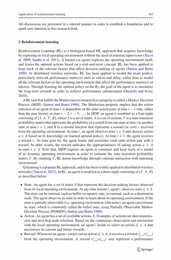
2.1 Q-learning model
Q-learning defines a Q-function Qit (s
it , ai
t ), which is also called a state-action function. TheQ-function estimates Q-values, which are the long-term rewards that an agent can expectto receive for each possible action ai
t ∈ A taken in state sit ∈ S. An agent i maintains a
Q-table that keeps track of Q-values for each possible state-action pair, so there are |S|× |A|entries. Subsequently, based on these Q-values, the agent derives an optimal policy π thatdefines the best-known action ai
t , which has the maximum Q-value for each state sit . For each
state-action pair (sit , ai
t ) at time t , the Q-value is updated using Q-function as follows:
Qit+1
(si
t , ait
)← (1− α) Qi
t
(si
t , ait
)+ α
[r i
t+1
(si
t+1
)+ γ max
a∈AQi
t
(si
t+1, a)]
(1)
where 0 ≤ α ≤ 1 is learning rate, and 0 ≤ γ ≤ 1 is discount factor. Higher learning rate α
indicates higher speed of learning, and it is normally dependent on the level of dynamicityin the operating environment. Note that, too high a learning rate may cause fluctuations inQ-values. If α = 1, the agent solely relies on its newly estimated Q-value r i
t+1(sit+1) +
γ maxa∈A
Qit (s
it+1, a), and forgets its current Q-value Qi
t (sit , ai
t ). On the other hand, γ enables
the agent to adjust its preference on the long-term future rewards. Unless γ = 1 in whichboth delayed and discounted rewards are given the same weight, the agent always gives morepreference to delayed rewards.
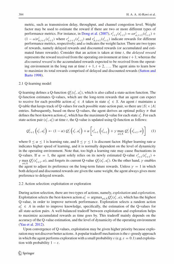
2.2 Action selection: exploitation or exploration
During action selection, there are two types of actions, namely, exploitation and exploration.Exploitation selects the best-known action ai
t = argmaxa∈A Qit (s
it , a), which has the highest
Q-value, in order to improve network performance. Exploration selects a random actionai
t ∈ A in order to improve knowledge, specifically, the estimation of the Q-values forall state-action pairs. A well-balanced tradeoff between exploitation and exploration helpsto maximize accumulated rewards as time goes by. This tradeoff mainly depends on theaccuracy of the Q-value estimation, and the level of dynamicity of the operating environment(Yau et al. 2012).
Upon convergence of Q-values, exploitation may be given higher priority because explo-ration may not discover better actions. A popular tradeoff mechanism is the ε-greedy approachin which the agent performs exploration with a small probability ε (e.g. ε = 0.1) and exploita-tion with probability 1− ε.
123
Application of reinforcement learning 385
The ε-greedy approach may not be suitable in some scenarios because exploration selectsnon-optimal actions randomly with equal probability, hence the worst action with the lowestQ-value may be chosen (Sutton and Barto 1998). A popular softmax approach based onthe Boltzmann distribution has been applied to choose non-optimal actions for exploration,and actions with higher Q-values are given higher priorities (Sutton and Barto 1998). Forinstance, in Dowling et al. (2005), a node i chooses its next-hop neighbor node ai
t ∈ A usingBoltzmann distribution with probability:
P(
sit , ai
t
)= e−Qi
t(sit ,a
it)/T
∑a∈A e−Qi
t(sit ,a
)/T
(2)
where A represents a set of node i’s neighbor nodes; and T is the temperature factor thatdetermines the level of exploration. Higher T value indicates higher possibility of exploringnon-optimal routes, whereas lower T value indicates higher possibility of exploiting optimalroutes.
In Bhorkar et al. (2012), a node i chooses its routing decision ait based on the historical
information as follows:
ε(
sit
)= 1
cit(si
t)+ 1
(3)
where cit (s
it ) is a counter that represents the number of successful packet transmissions
from node i to next-hop neighbor node sit ∈ Si until time t . Subsequently, with probability
1 − ε(sit ), node i chooses its routing decision ai
t = argmaxa∈A(sit )
Qit (s
it , a), while with
a smaller probability ε(sit ), node i chooses its routing decision ai
t ∈ A(sit ) equally with
probability ε(sit )/|A(si
t )|.In Liang et al. (2008), a node i adjusts its level of exploration according to the level of
dynamicity in the operating environment, particularly node mobility. The node computes theexploration probability as follows:
εi = na,Ti + nd,T
i
nTi
(4)
where na,Ti and nd,T
i are the number of nodes that appear and disappear within node i’stransmission range, respectively; nT
i is the number of node i’s neighbor nodes; and T is atime window. Hence, higher εi indicates a highly mobile network, and so RL requires moreexplorations.
2.3 Q-learning algorithm
Figure 1 shows the traditional Q-learning algorithm presented in Sects. 2.1 and 2.2.
3 Routing in distributed wireless networks
Routing is a key component in distributed wireless networks that enables a source node tosearch and establish route(s) to the destination node through a set of intermediate nodes. Theobjectives of the routing schemes are mainly dependent on the type of operating environmentand the underlying network, particularly its characteristics and requirements. This sectionreviews the concepts of routing in various types of distributed wireless networks, and the
123

386 H. A. A. Al-Rawi et al.
Fig. 1 The traditional Q-learning algorithm at agent i
advantages brought about by RL to routing. With respect to routing, Sect. 3.1 reviews severalmajor types of distributed wireless networks, particularly network characteristics, routingchallenges, and the advantages brought about by RL to routing. Section 3.2 provides anoverview of the application of RL to routing in distributed wireless networks, and a generalformulation of the routing problem using RL.
3.1 Types of distributed wireless networks
This section presents four types of distributed wireless networks, namely wireless ad hocnetworks, wireless sensor networks, cognitive radio networks, and delay tolerant networks.Table 1 summarizes each type of these networks.
3.1.1 Wireless ad hoc networks
A wireless ad hoc network is comprised of self-configuring static or mobile nodes. Two maintypes of wireless ad hoc networks are static ad hoc networks and Mobile Ad hoc NETworks(MANETs) (Toh 2001; Boukerche 2009).
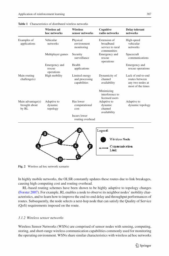
Figure 2 shows a wireless ad hoc network scenario. Nodes within the range of each other(e.g. A and B) may communicate directly; and out-of-range nodes (e.g. A and F) may usea routing scheme to search for a route, comprised of intermediate nodes, from node (A) tonode (F). The routing scheme uses a cost metric to compute the best possible route, such asthe shortest route and route with the lowest end-to-end delay.
The main routing challenge in wireless ad hoc networks is the dynamic topology causedby nodes’ mobility. For instance, in Fig. 2, source node (A) establishes a route (A-H-G-F)to destination node (F). Suppose, node (H) moves and becomes out-of-range from node (A)resulting in link breakage, then node (A) searches for another route to node (F). The packetend-to-end delay and packet loss rate are dependent on the effectiveness of the routing scheme.Furthermore, in link-state routing schemes, such as Optimized Link State Routing (OLSR)(Clausen and Jacquet 2003), each node maintains a route to every other nodes in the network.
123
Application of reinforcement learning 387
Table 1 Characteristics of distributed wireless networks
Wireless adhoc networks
Wirelesssensor networks
Cognitiveradio networks
Delay tolerantnetworks
Examples ofapplications
Vehicularnetworks
Physicalenvironmentmonitoring
Extension ofbroadbandservice to ruralcommunities
High-speedvehicularnetworks
Multiplayer games Securitysurveillance
Emergency andrescueoperations
Spacecraftcommunications
Emergency andrescueoperations
Healthapplications
Emergency andrescue operations
Main routingchallenge(s)
High mobility Limited energyand processingcapabilities
Dynamicity ofchannelavailability
Lack of end-to-endroutes betweenany two nodes atmost of the times
Minimizinginterference tolicensed users
Main advantage(s)brought aboutby RL
Adaptive todynamictopology
Has lowercomputationalcost
Adaptive todynamicchannelavailability
Adaptive todynamic topology
Incurs lowerrouting overhead
Fig. 2 Wireless ad hoc network scenario
In highly mobile networks, the OLSR constantly updates these routes due to link breakages,causing high computing cost and routing overhead.
RL-based routing schemes have been shown to be highly adaptive to topology changes(Forster 2007). For example, RL enables a node to observe its neighbor nodes’ mobility char-acteristics, and to learn how to improve the end-to-end delay and throughput performances ofroutes. Subsequently, the node selects a next-hop node that can satisfy the Quality of Service(QoS) requirements imposed on the route.
3.1.2 Wireless sensor networks
Wireless Sensor Networks (WSNs) are comprised of sensor nodes with sensing, computing,storing, and short-range wireless communication capabilities commonly used for monitoringthe operating environment. WSNs share similar characteristics with wireless ad hoc networks
123
388 H. A. A. Al-Rawi et al.
Fig. 3 WSN scenario
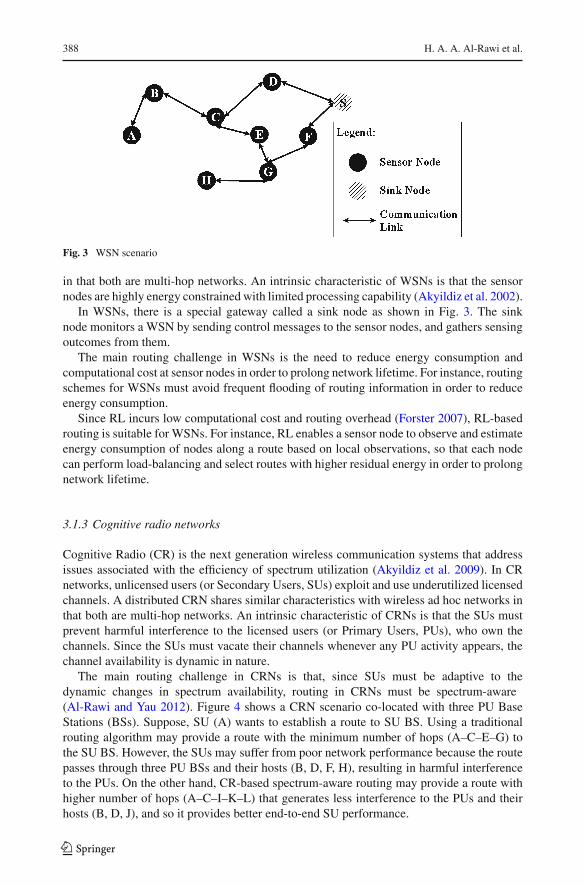
in that both are multi-hop networks. An intrinsic characteristic of WSNs is that the sensornodes are highly energy constrained with limited processing capability (Akyildiz et al. 2002).
In WSNs, there is a special gateway called a sink node as shown in Fig. 3. The sinknode monitors a WSN by sending control messages to the sensor nodes, and gathers sensingoutcomes from them.
The main routing challenge in WSNs is the need to reduce energy consumption andcomputational cost at sensor nodes in order to prolong network lifetime. For instance, routingschemes for WSNs must avoid frequent flooding of routing information in order to reduceenergy consumption.
Since RL incurs low computational cost and routing overhead (Forster 2007), RL-basedrouting is suitable for WSNs. For instance, RL enables a sensor node to observe and estimateenergy consumption of nodes along a route based on local observations, so that each nodecan perform load-balancing and select routes with higher residual energy in order to prolongnetwork lifetime.
3.1.3 Cognitive radio networks
Cognitive Radio (CR) is the next generation wireless communication systems that addressissues associated with the efficiency of spectrum utilization (Akyildiz et al. 2009). In CRnetworks, unlicensed users (or Secondary Users, SUs) exploit and use underutilized licensedchannels. A distributed CRN shares similar characteristics with wireless ad hoc networks inthat both are multi-hop networks. An intrinsic characteristic of CRNs is that the SUs mustprevent harmful interference to the licensed users (or Primary Users, PUs), who own thechannels. Since the SUs must vacate their channels whenever any PU activity appears, thechannel availability is dynamic in nature.
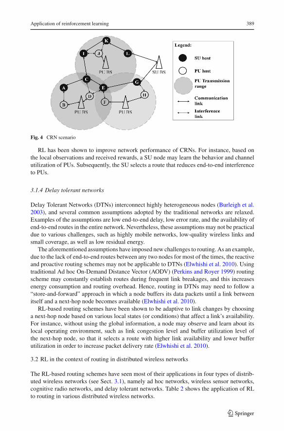
The main routing challenge in CRNs is that, since SUs must be adaptive to thedynamic changes in spectrum availability, routing in CRNs must be spectrum-aware(Al-Rawi and Yau 2012). Figure 4 shows a CRN scenario co-located with three PU BaseStations (BSs). Suppose, SU (A) wants to establish a route to SU BS. Using a traditionalrouting algorithm may provide a route with the minimum number of hops (A–C–E–G) tothe SU BS. However, the SUs may suffer from poor network performance because the routepasses through three PU BSs and their hosts (B, D, F, H), resulting in harmful interferenceto the PUs. On the other hand, CR-based spectrum-aware routing may provide a route withhigher number of hops (A–C–I–K–L) that generates less interference to the PUs and theirhosts (B, D, J), and so it provides better end-to-end SU performance.
123
Application of reinforcement learning 389
Fig. 4 CRN scenario
RL has been shown to improve network performance of CRNs. For instance, based onthe local observations and received rewards, a SU node may learn the behavior and channelutilization of PUs. Subsequently, the SU selects a route that reduces end-to-end interferenceto PUs.
3.1.4 Delay tolerant networks
Delay Tolerant Networks (DTNs) interconnect highly heterogeneous nodes (Burleigh et al.2003), and several common assumptions adopted by the traditional networks are relaxed.Examples of the assumptions are low end-to-end delay, low error rate, and the availability ofend-to-end routes in the entire network. Nevertheless, these assumptions may not be practicaldue to various challenges, such as highly mobile networks, low-quality wireless links andsmall coverage, as well as low residual energy.
The aforementioned assumptions have imposed new challenges to routing. As an example,due to the lack of end-to-end routes between any two nodes for most of the times, the reactiveand proactive routing schemes may not be applicable to DTNs (Elwhishi et al. 2010). Usingtraditional Ad hoc On-Demand Distance Vector (AODV) (Perkins and Royer 1999) routingscheme may constantly establish routes during frequent link breakages, and this increasesenergy consumption and routing overhead. Hence, routing in DTNs may need to follow a“store-and-forward” approach in which a node buffers its data packets until a link betweenitself and a next-hop node becomes available (Elwhishi et al. 2010).
RL-based routing schemes have been shown to be adaptive to link changes by choosinga next-hop node based on various local states (or conditions) that affect a link’s availability.For instance, without using the global information, a node may observe and learn about itslocal operating environment, such as link congestion level and buffer utilization level ofthe next-hop node, so that it selects a route with higher link availability and lower bufferutilization in order to increase packet delivery rate (Elwhishi et al. 2010).
3.2 RL in the context of routing in distributed wireless networks
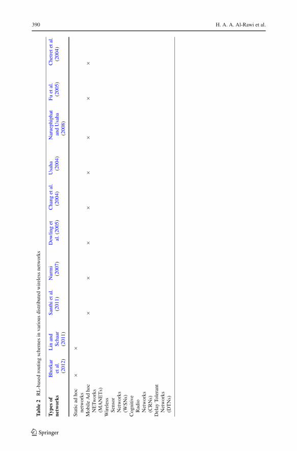
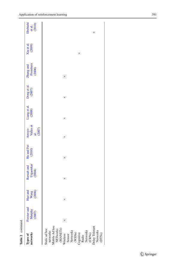
The RL-based routing schemes have seen most of their applications in four types of distrib-uted wireless networks (see Sect. 3.1), namely ad hoc networks, wireless sensor networks,cognitive radio networks, and delay tolerant networks. Table 2 shows the application of RLto routing in various distributed wireless networks.
123
390 H. A. A. Al-Rawi et al.
Tabl
e2
RL
-bas
edro
utin
gsc
hem
esin
vari
ous
dist
ribu
ted
wir
eles
sne
twor
ks
Typ
esof
netw
orks
Bho
rkar
etal
.(2
012)
Lin
and
Scha
ar(2
011)
Sant
hiet
al.
(201
1)N
urm
i(2
007)
Dow
ling
etal
.(20
05)
Cha
nget
al.
(200
4)U
saha
(200
4)N
arue
phip
hat
and
Usa
ha(2
008)
Fuet
al.
(200
5)C
hetr
etet
al.
(200
4)
Stat
icad
hoc
netw
orks
××
Mob
ileA
dho
cN
ETw
orks
(MA
NE
Ts)
××
××
××
××
Wir
eles
sSe
nsor
Net
wor
ks(W
SNs)
Cog
nitiv
eR
adio
Net
wor
ks(C
RN
s)D
elay
Tole
rant
Net
wor
ks(D
TN
s)
123
Application of reinforcement learning 391
Tabl
e2
cont
inue
d
Typ
esof
netw
orks
Fors
ter
and
Mur
phy
(200
7)
Hao
and
Wan
g(2
006)
Bar
uah
and
Urg
aonk
ar(2
004)
Hu
and
Fei
(201
0)A
rroy
o-V
alle
set
al.
(200
7)
Lia
nget
al.
(200
8)D
ong
etal
.(2
007)
Zha
ngan
dFr
omhe
rz(2
006)
Xia
etal
.(2
009)
Elw
hish
iet
al.
(201
0)
Stat
icad
hoc
netw
orks
Mob
ileA
dho
cN
ETw
orks
(MA
NE
Ts)
Wir
eles
sSe
nsor
Net
wor
ks(W
SNs)
××
××
××
××
Cog
nitiv
eR
adio
Net
wor
ks(C
RN
s)
×
Del
ayTo
lera
ntN
etw
orks
(DT
Ns)
×
123
392 H. A. A. Al-Rawi et al.
Routing in distributed wireless networks has been approached using RL so that each nodemakes local decision, with regards to next-hop or link selection as part of a route, in order tooptimize network performance. In routing, the RL approach enables a node to:
a. estimate the dynamic link cost. This characteristic allows a node to learn about andadapt to its dynamic local operating environment.
b. search for the best possible route using information observed from the local operatingenvironment only.
c. incorporate a wide range of factors that affect the routing performance.
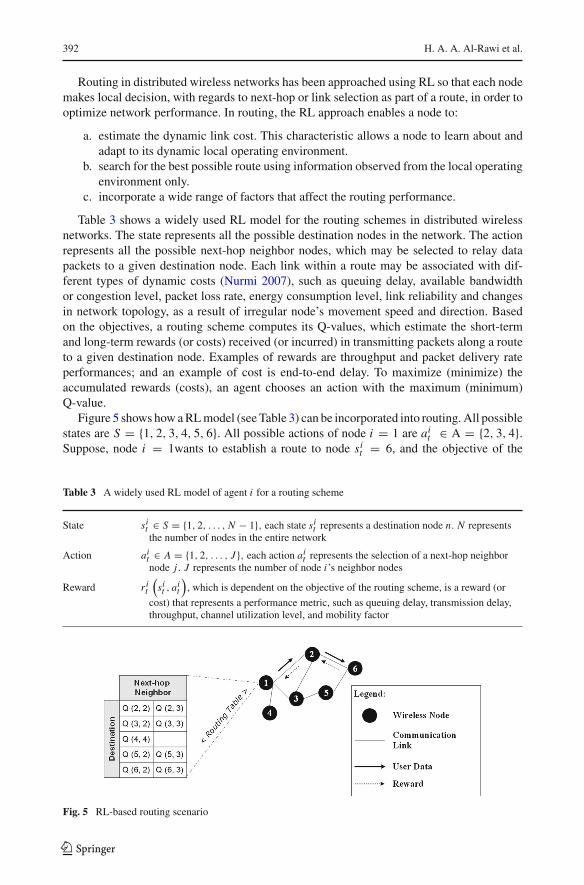
Table 3 shows a widely used RL model for the routing schemes in distributed wirelessnetworks. The state represents all the possible destination nodes in the network. The actionrepresents all the possible next-hop neighbor nodes, which may be selected to relay datapackets to a given destination node. Each link within a route may be associated with dif-ferent types of dynamic costs (Nurmi 2007), such as queuing delay, available bandwidthor congestion level, packet loss rate, energy consumption level, link reliability and changesin network topology, as a result of irregular node’s movement speed and direction. Basedon the objectives, a routing scheme computes its Q-values, which estimate the short-termand long-term rewards (or costs) received (or incurred) in transmitting packets along a routeto a given destination node. Examples of rewards are throughput and packet delivery rateperformances; and an example of cost is end-to-end delay. To maximize (minimize) theaccumulated rewards (costs), an agent chooses an action with the maximum (minimum)Q-value.
Figure 5 shows how a RL model (see Table 3) can be incorporated into routing. All possiblestates are S = {1, 2, 3, 4, 5, 6}. All possible actions of node i = 1 are ai
t ∈ A = {2, 3, 4}.Suppose, node i = 1wants to establish a route to node si
t = 6, and the objective of the
Table 3 A widely used RL model of agent i for a routing scheme
State sit ∈ S = {1, 2, . . . , N − 1}, each state si
t represents a destination node n. N representsthe number of nodes in the entire network
Action ait ∈ A = {1, 2, . . . , J }, each action ai
t represents the selection of a next-hop neighbornode j . J represents the number of node i’s neighbor nodes
Reward r it
(sit , ai
t
), which is dependent on the objective of the routing scheme, is a reward (or
cost) that represents a performance metric, such as queuing delay, transmission delay,throughput, channel utilization level, and mobility factor
Fig. 5 RL-based routing scenario
123

Application of reinforcement learning 393
routing scheme is to find a route that provides the highest throughput performance. Nodei may choose to send its packets to its neighbor node ai
t = 2, and receives a rewardfrom node ai
t = 2 that estimates throughput achieved by the route from upstream nodeai
t = 2 to destination node sit = 6, specifically route (2–6). Subsequently, node i updates
its Q-value for state sit = 6 via action ai
t = 2 using Q-function (see Eq. 1), specificallyQi
t
(si
t = 6, ait = 2
). Likewise, when node i sends its data packets to node ai
t = 3, itreceives a reward that estimates the throughput from upstream node ai
t = 3, which canbe either (3–2–6) or (3–5–6), and updates Qi
t
(si
t = 6, ait = 3
). Note that, whether route
(3–2–6) or (3–5–6) is chosen by upstream node ait = 3 is dependent on the Q-values of
Qi=3t
(si=3
t = 6, ai=3t = 2
)and Qi=3
t
(si=3
t = 6, ai=3t = 5
)at node ai
t = 3, and the upstreamnode that provides the maximum Q-value is the exploitation action. The matrix in Fig. 5 showsan example of routing table (or Q-table) being constantly updated at node i . Node i keepstrack of the Q-values of all possible destinations through its next-hop neighbor nodes in itsQ-table.
4 Reinforcement learning models for routing
RL models have been applied to routing schemes in various distributed wireless networks.The RL models are: Q-routing, Multi-Agent Reinforcement Learning (MARL), and PartiallyObservable Markov Decision Process (POMDP). The rest of this section discusses the RLmodels.
4.1 Q-routing model
Boyan and Littman (1994) propose Q-routing, which is based on the traditional Q-learningmodel (Sutton and Barto 1998). In Q-routing, a node chooses a next-hop node, which has theminimum end-to-end delay, in order to mitigate link congestion (Ouzecki and Jevtic 2010;Chang et al. 2004). The traditional Q-routing approach has also been adopted as a generalapproach to improve network performance in Zhang and Fromherz (2006).
In Q-routing, the state sit represents a destination node in the network. The action ai
trepresents the selection of a next-hop neighbor node to relay data to a destination node si
t .Each link of a route is associated with a dynamic delay cost comprised of queuing andtransmission delays. Subsequently, for each state-action pair (or destination and next-hopneighbor node pair), a node computes its Q-value, which estimates the end-to-end delay fortransmitting packets along a route to a destination node si
t . Specifically, at time instant t + 1,a particular node i updates its Q-value Qi
t (sit , j) to a destination node si
t via a next-hopneighbor node ai
t = j . Hence, Eq. (1) is rewritten as follows:
Qit+1
(si
t , j)← (1− α) Qi
t
(si
t , j)+ α
[r i
t+1
(si
t+1, j)+ min
k∈a jt
Q jt
(s j
t , k)]
(5)
where 0 ≤ α ≤ 1 is the learning rate; r it+1(s
it+1, j) = di
qu,t+1+ di, jtr,t+1 represents two types
of delays, specifically diqu,t+1 is the queuing delay at node i , and di, j
tr,t+1 is the transmission
delay between node i and its next-hop neighbor node j ; and Q jt (s
jt , k), which is a Q-value
received from next-hop neighbor node j , is the estimated end-to-end delay along the routefrom node j’s next-hop neighbor node k ∈ a j
t to the destination node.
123
394 H. A. A. Al-Rawi et al.
Referring to Fig. 5, suppose node i = 1wants to establish a route to node sit = 6 using
the Q-routing model. Node i = 1 may choose its next-hop neighbor node ait = j = 2
to forward its data packets. When node i sends its data packets to node j = 2, it receivesfrom neighbor node j = 2 an estimate of min
k∈a jt
Q jt (s
jt , k) that represents the estimated
minimum end-to-end delay from node j to destination nodesit . Node i = 1 also measures
its queuing delay diqu,t+1 and transmission delay di, j
tr,t+1 between itself and neighbor node
j = 2. Subsequently, using Eq. (5), node i updates its Q-value, Qit (s
it = 6, ai
t = 2) thatrepresents the end-to-end delay from itself to destination node si
t = 6 through the chosennext-hop neighbor node ai
t = 2.
4.2 Multi-agent reinforcement learning model
The traditional RL model, which is greedy in nature, provides local optimizations regardlessof the global performance; and so, it is not sufficient to achieve global optimizations or anetwork-wide QoS provisioning. This can be explained as follows: since nodes share a com-mon operating environment in wireless networks, a node’s neighbor nodes may take actionsthat affect its own performance due to channel contention. In Multi-Agent ReinforcementLearning (MARL), in addition to learning locally using the traditional RL model, each nodeexchanges locally observed information with neighboring nodes through collaboration inorder to achieve global optimizations. This helps the nodes to consider not only their ownperformance, but also others’ performance. Hence, the Multi-Agent Reinforcement Learn-ing (MARL) model extends the traditional RL model through fostering collaboration amongneighboring nodes so that a system-wide optimization problem can be decomposed into aset of distributed problems solved by individual nodes in a distributed manner.
Referring to Fig. 5, node i = 1 constantly exchanges knowledge (i.e. Q-values andrewards) with neighbor nodes j = 2, 3 and 4. As an example, in Dowling et al. (2005), theMARL-based routing scheme addresses a routing challenge in which a node i selects itsnext-hop neighbor node j with the objective of increasing network throughput and packetdelivery rate in a heterogeneous mobile ad hoc network (see Sect. 3.1.1). Each node maypossess different capabilities in solving the routing problem in a heterogeneous environment.Hence, the nodes share their knowledge (i.e. route cost) through message exchange. Theexchanged route cost is subsequently applied by a node i to update its Q-values so that anaction, which maximizes the rewards of itself and its neighboring nodes, is chosen.
4.3 Partially observable Markov decision process model
The Partial Observable Markov Decision Process (POMDP) model extends the Q-routingand Multi-agent RL model. In POMDP-based routing model, a node is not able to clearlyobserve its operating environment. Since the state is unknown, the node must estimate thestate. For instance, the state of a node may incorporate its next-hop neighbor node’s localparameters, such as the forwarding selfishness, residual energy, and congestion level.
As an example, in Nurmi (2007), the routing scheme addresses a routing challenge inwhich a node i selects its next-hop neighbor node j with the objective of minimizing energyconsumption. Node j’s forwarding decision, which is based on its local parameters (or states)such as the forwarding selfishness, residual energy and congestion level, is unclear to nodei . Additionally, node j’s decision is stochastic in nature. Hence, node j’s information isunknown to node i . The routing scheme is formulated as a POMDP problem in which node i
123
Application of reinforcement learning 395
estimates the probability distribution of the local parameters based on its previous estimationand its observed historical actions H j
t of node j .
5 New features
This section presents the new features that have been incorporated into the traditional RL-based routing models in order to further enhance network performance.
5.1 Achieving balance between exploitation and exploration
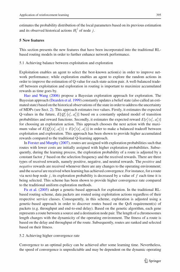
Exploitation enables an agent to select the best-known action(s) in order to improve net-work performance; while exploration enables an agent to explore the random actions inorder to improve the estimation of Q-value for each state-action pair. A well-balanced trade-off between exploitation and exploration in routing is important to maximize accumulatedrewards as time goes by.
Hao and Wang (2006) propose a Bayesian exploration approach for exploration. TheBayesian approach (Dearden et al. 1999) constantly updates a belief state (also called an esti-mated state) based on the historical observations of the state in order to address the uncertaintyof MDPs (see Sect. 2). This approach estimates two values. Firstly, it estimates the expectedQ-values in the future, E[Qi
t
(si
t , ait
)] based on a constantly updated model of transitionprobabilities and reward functions. Secondly, it estimates the expected reward E[r i
t (sit , ai
t )]for choosing an exploration action. This approach chooses the next action with the maxi-mum value of E[Qi
t (sit , ai
t )] + E[r it (s
it , ai
t )] in order to make a balanced tradeoff betweenexploitation and exploration. This approach has been shown to provide higher accumulatedrewards compared to the traditional Q-learning approach.
In Forster and Murphy (2007), routes are assigned with exploration probabilities such thatroutes with lower costs are initially assigned with higher exploration probabilities. Subse-quently, during the learning process, the exploration probability of a route is adjusted by aconstant factor f based on the selection frequency and the received rewards. There are threetypes of received rewards, namely positive, negative, and neutral rewards. The positive andnegative rewards are received whenever there are any changes to the operating environment;and the neutral are received when learning has achieved convergence. For instance, for a routevia next-hop node j , its exploration probability is decreased by a value of f each time it isbeing selected. This scheme has been shown to provide higher convergence rate comparedto the traditional uniform exploration methods.
Fu et al. (2005) adopt a genetic-based approach for exploration. In the traditional RL-based routing scheme, data packets are routed using exploitation actions regardless of theirrespective service classes. Consequently, in this scheme, exploration is adjusted using agenetic-based approach in order to discover routes based on the QoS requirement(s) ofpackets (e.g. throughput and end-to-end delay). Based on the genetic algorithm, each generepresents a route between a source and a destination node pair. The length of a chromosomeslength changes with the dynamicity of the operating environment. The fitness of a route isbased on the delay and throughput of the route. Subsequently, routes are ranked and selectedbased on their fitness.
5.2 Achieving higher convergence rate
Convergence to an optimal policy can be achieved after some learning time. Nevertheless,the speed of convergence is unpredictable and may be dependent on the dynamic operating
123

396 H. A. A. Al-Rawi et al.
environment. Traditionally, the learning rate α is used to adjust the speed of convergence.Higher learning rate may increase the convergence speed; however, the Q-value may fluctuate,particularly when the dynamicity of the operating environment is high because the Q-valueis now dependent more on its recent estimates, rather than its previous experience.
Nurmi (2007) applies a stochastic learning algorithm, namely Win-or-Learn-Fast PolicyHill Climbing (WoLF-PHC) (Bowling and Veloso 2002), to adjust the learning rate dynami-cally based on the dynamicity of the operating environment in distributed wireless networks.The algorithm defines Winning and Losing as receiving higher and lower rewards than itsexpectations, respectively. When the algorithm is winning, the learning rate is set to a lowervalue, and vice-versa. The reason is that, when a node is winning, it should be cautious inchanging its policy because more time should be given to the other nodes to adjust their ownpolicies in favor of this winning. On the other hand, when a node is losing, it should adaptfaster to any changes in the operating environment because its performance (or rewards) islower than expected.
Kumar and Miikkulainen (1997) apply a dual RL-based approach to speed up the con-vergence rate by updating the Q-values of previous state (i.e. source node) and next state(i.e. destination node) simultaneously although this may increase the routing overhead. Thetraditional Q-routing model updates the Q-values in regards to the destination node (seeSect. 4.1). On the other hand, dual RL-based Q-routing model updates Q-values in regards todestination and source nodes. Since the dual RL-based approach updates Q-values of a routein both directions, it enables nodes along a route to make decisions on next-hop selection forboth source and destination nodes while increasing the speed of convergence.
Hu and Fei (2010) use a system model to estimate the converged Q-values of all actions sothat it may not be necessary to update Q-values only after taking the corresponding actions.This is achieved through running virtual experiment or simulation to update Q-values using asystem model. The system model is comprised of a state transition probability matrix T (seeSect. 2), which is estimated using historical data of each link’s successful and unsuccessfultransmission rate based on the outgoing traffic of next-hop neighbor nodes.
5.3 Detecting the convergence of Q-values
When the Q-values have achieved convergence, further exploration may not change theQ-values, and so an exploitation action should be chosen. Hence, the detection of the con-vergence of Q-values helps to enhance network-wide performance.
Forster and Murphy (2007) propose two techniques to detect the convergence of Q-valuesfor each route with the objective of enhancing the learning process so that the knowledge issufficiently comprehensive. Specifically, the first technique ensures the convergence of eachroute at the unit level, while the second technique enhances the convergence of N differentroutes at the system level. The first technique assumes that the Q-value of a route has achievedconvergence when the route receives M static (or unchanged) rewards. On the other hand,the second technique requires at least N routes have been explored, which ensures thatconvergence is achieved at the system level. Combining both techniques, the convergence isachieved when there are N routes receiving M static rewards.
5.4 Storing Q-values efficiently
When the number of states (e.g. destination nodes) increases, memory requirement to store theQ-values for all state-action pairs may increase exponentially. Storing the Q-values efficientlymay reduce the memory requirement.
123
Application of reinforcement learning 397
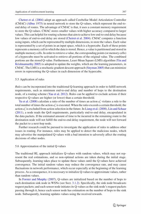
Chetret et al. (2004) adopt an approach called Cerebellar Model Articulation Controller(CMAC) (Albus 1975) in neural network to store the Q-values, which represent the end-to-end delay of routes. The advantage of CMAC is that, it uses a constant memory requirementto store the Q-values. CMAC stores smaller values with higher accuracy compared to largervalues. This can helpful for routing schemes that aim to achieve low end-to-end delay becauselow values of end-to-end delay are stored (Chetret et al. 2004). CMAC computes a functionusing inputs, which can be represented by multiple dimensions, to store the values. Each valueis represented by a set of points in an input space, which is a hypercube. Each of these pointsrepresents a memory cell in which the data is stored. Hence, a value is partitioned and stored inmultiple memory cells. In order to retrieve a value, the corresponding points (or memory cells)of a hypercube must be activated to retrieve all portions of the original value. The combinedportions are the stored Q-value. Furthermore, Least-Mean Square (LMS) algorithm (Yin andKrishnamurthy 2005) is adopted to update the weights, which are the learning parameters, inCMAC. The LMS is a stochastic gradient descent approach (Snyman 2005) that can minimizeerrors in representing the Q-values in each dimension of the hypercube.
5.5 Application of rules
Rules can be incorporated into the traditional Q-learning approach in order to fulfill networkrequirements, such as minimum end-to-end delay and number of hops to the destinationnode, of a routing scheme (Yau et al. 2012). Rules can be applied to exclude actions if theirrespective Q-values are higher (or lower) than a certain threshold.
Yu et al. (2008) calculate a ratio of the number of times an action ait violates a rule to the
total number of times the action ait is executed. When the ratio exceeds a certain threshold, the
action ait is excluded from action selection in the future. In Liang et al. (2008), Lin and Schaar
(2011), a node reads the QoS requirements, particularly end-to-end delay, encapsulated inthe data packets. If the estimated amount of time to be incurred in the remaining route to thedestination node will not fulfill the end-to-end delay requirement, the node will not forwardthe packet to a next-hop node.
Further research could be pursued to investigate the application of rules to address otherissues in routing. For instance, rules may be applied to detect the malicious nodes, whichmay advertise the manipulated Q-values with a bad intention to adversely affect the routingdecisions of other nodes.
5.6 Approximation of the initial Q-values
The traditional RL approach initializes Q-values with random values, which may not rep-resent the real estimations, and so non-optimal actions are taken during the initial stage.Subsequently, learning takes place to update these values until the Q-values have achievedconvergence. The initial random values may reduce the convergence rate, and may causefluctuations in network performance, which occur especially at the beginning of the learningprocess. As a consequence, it is necessary to initialize Q-values to approximate values, ratherthan random values.
In Forster and Murphy (2007), Q-values are initialized based on the number of hops toeach destination sink node in WSNs (see Sect. 3.1.2). Specifically, the sink node broadcastsrequest packets; and each sensor node initiates its Q-values as the sink node’s request packetspassing through it, hence each sensor node has estimation on the number of hops to the sinknode. Subsequently, learning updates values using the received rewards.
123
398 H. A. A. Al-Rawi et al.
6 Application of reinforcement learning to routing in distributed wireless networks
This section presents how various routing schemes have been approached using RL to providenetwork performance enhancement. We describe the main purpose of each scheme, and itsRL model.
6.1 Q-routing model
This section discusses the routing schemes that adopt the Q-routing model (see Sect. 4.1).
6.1.1 Q-routing approach with forward and backward exploration
Dual RL-based Q-routing (Kumar and Miikkulainen 1997), which is an extension of thetraditional Q-routing model, enhances network performance and convergence speed (seeSect. 5.2). Xia et al. (2009) also apply a Dual RL-based Q-routing approach in CRNs (seeSect. 3.1.3), and it has been shown to reduce end-to-end delay. In CRNs, the availabilityof a channel is dynamic, and it is dependent on the PU activity level. The purpose of therouting scheme is to enable a node to select a next-hop neighbor node with higher numberof available channels. Higher number of available channels reduces channel contention, andhence reduces the MAC layer delay.
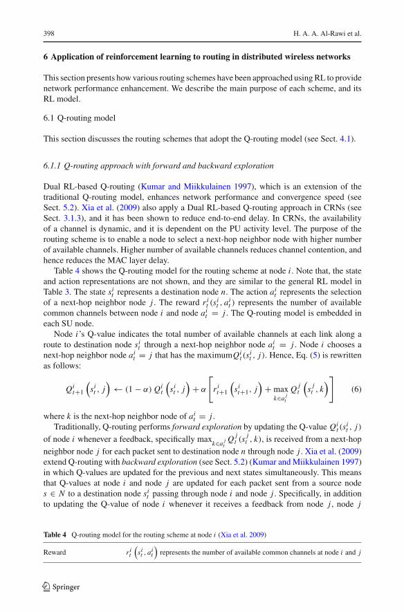
Table 4 shows the Q-routing model for the routing scheme at node i . Note that, the stateand action representations are not shown, and they are similar to the general RL model inTable 3. The state si
t represents a destination node n. The action ait represents the selection
of a next-hop neighbor node j . The reward r it (s
it , ai
t ) represents the number of availablecommon channels between node i and node ai
t = j . The Q-routing model is embedded ineach SU node.
Node i’s Q-value indicates the total number of available channels at each link along aroute to destination node si
t through a next-hop neighbor node ait = j . Node i chooses a
next-hop neighbor node ait = j that has the maximumQi
t (sit , j). Hence, Eq. (5) is rewritten
as follows:
Qit+1
(si
t , j)← (1− α) Qi
t
(si
t , j)+ α
[r i
t+1
(si
t+1, j)+max
k∈a jt
Q jt
(s j
t , k)]
(6)
where k is the next-hop neighbor node of ait = j .
Traditionally, Q-routing performs forward exploration by updating the Q-value Qit (s
it , j)
of node i whenever a feedback, specifically maxk∈a j
tQ j
t (sjt , k), is received from a next-hop
neighbor node j for each packet sent to destination node n through node j . Xia et al. (2009)extend Q-routing with backward exploration (see Sect. 5.2) (Kumar and Miikkulainen 1997)in which Q-values are updated for the previous and next states simultaneously. This meansthat Q-values at node i and node j are updated for each packet sent from a source nodes ∈ N to a destination node si
t passing through node i and node j . Specifically, in additionto updating the Q-value of node i whenever it receives a feedback from node j , node j
Table 4 Q-routing model for the routing scheme at node i (Xia et al. 2009)
Reward r it
(sit , ai
t
)represents the number of available common channels at node i and j
123
Application of reinforcement learning 399
also updates its Q-value whenever it receives forwarded packets from node i . Note that, thepackets are piggybacked with Q-values of node i into the forwarded packets to neighbornode j . Using this approach, node i has an updated Q-value to destination node si
t throughneighbor node j ; and node j has an updated Q-value to source node s through neighbor nodei . Hence, nodes along a route have updated Q-values of the route in both directions. The dualRL-based Q-routing approach has been shown to minimize end-to-end delay.
6.1.2 Q-routing approach with dynamic discount factor
The traditional RL approach has a static discount factor γ , which indicates the preferenceon the future long-term rewards. This enhanced Q-routing approach with dynamic discountfactor calculates the discount factor of each next-hop neighbor node, hence each of them mayhave different values of discount factor. This may provide a more accurate estimation on theQ-values of different next-hop neighbor nodes, which may have different characteristics andcapabilities.
Santhi et al. (2011) propose a Q-routing approach with dynamic discount factor to reducethe frequency of triggering the route discovery process due to link breakage in MANETs.The proposed routing scheme aims to establish routes with high robustness, which are lesslikely to fail, and it has been shown to reduce end-to-end delay and increase packet deliveryrate. This is achieved by selecting a reliable next-hop neighbor node based on three factors,which are considered in the estimation of discount factor γ , namely link stability, bandwidthefficiency, and node’s residual energy. Note that, the link stability is dependent on the nodemobility.
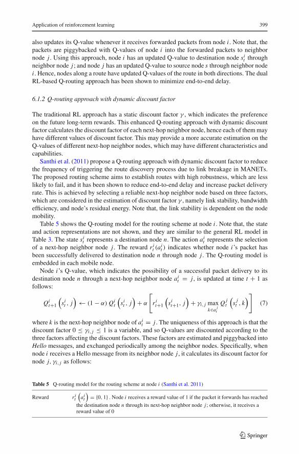
Table 5 shows the Q-routing model for the routing scheme at node i . Note that, the stateand action representations are not shown, and they are similar to the general RL model inTable 3. The state si
t represents a destination node n. The action ait represents the selection
of a next-hop neighbor node j . The reward r it (a
it ) indicates whether node i’s packet has
been successfully delivered to destination node n through node j . The Q-routing model isembedded in each mobile node.
Node i’s Q-value, which indicates the possibility of a successful packet delivery to itsdestination node n through a next-hop neighbor node ai
t = j , is updated at time t + 1 asfollows:
Qit+1
(si
t , j)← (1− α) Qi
t
(si
t , j)+ α
[r i
t+1
(si
t+1, j)+ γi, j max
k∈a jt
Q jt
(s j
t , k)]
(7)
where k is the next-hop neighbor node of ait = j . The uniqueness of this approach is that the
discount factor 0 ≤ γi, j ≤ 1 is a variable, and so Q-values are discounted according to thethree factors affecting the discount factors. These factors are estimated and piggybacked intoHello messages, and exchanged periodically among the neighbor nodes. Specifically, whennode i receives a Hello message from its neighbor node j , it calculates its discount factor fornode j, γi, j as follows:
Table 5 Q-routing model for the routing scheme at node i (Santhi et al. 2011)
Reward r it
(ai
t
)= {0, 1} . Node i receives a reward value of 1 if the packet it forwards has reached
the destination node n through its next-hop neighbor node j ; otherwise, it receives areward value of 0
123
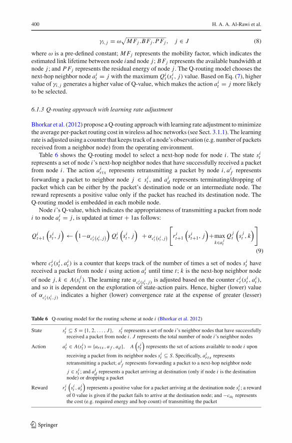
400 H. A. A. Al-Rawi et al.
γi, j = ω√
M Fj .B Fj .P Fj , j ∈ J (8)
where ω is a pre-defined constant; M Fj represents the mobility factor, which indicates theestimated link lifetime between node iand node j ; B Fj represents the available bandwidth atnode j ; and P Fj represents the residual energy of node j . The Q-routing model chooses thenext-hop neighbor node ai
t = j with the maximum Qit (s
it , j) value. Based on Eq. (7), higher
value of γi, j generates a higher value of Q-value, which makes the action ait = j more likely
to be selected.
6.1.3 Q-routing approach with learning rate adjustment
Bhorkar et al. (2012) propose a Q-routing approach with learning rate adjustment to minimizethe average per-packet routing cost in wireless ad hoc networks (see Sect. 3.1.1). The learningrate is adjusted using a counter that keeps track of a node’s observation (e.g. number of packetsreceived from a neighbor node) from the operating environment.
Table 6 shows the Q-routing model to select a next-hop node for node i . The state sit
represents a set of node i’s next-hop neighbor nodes that have successfully received a packetfrom node i . The action ai
rtx represents retransmitting a packet by node i, aif represents
forwarding a packet to neighbor node j ∈ sit , and ai
d represents terminating/dropping ofpacket which can be either by the packet’s destination node or an intermediate node. Thereward represents a positive value only if the packet has reached its destination node. TheQ-routing model is embedded in each mobile node.
Node i’s Q-value, which indicates the appropriateness of transmitting a packet from nodei to node ai
t = j , is updated at timet + 1as follows:
Qit+1
(si
t , j)←
(1−αci
t(sit , j
))
Qit
(si
t , j)+ αci
t(sit , j
)[
r it+1
(si
t+1, j)+max
k∈a jt
Q jt
(s j
t , k)]
(9)
where cit (s
it , ai
t ) is a counter that keeps track of the number of times a set of nodes sit have
received a packet from node i using action ait until time t ; k is the next-hop neighbor node
of node j, k ∈ A(s jt ). The learning rate αci
t (sit , j) is adjusted based on the counter ci
t (sit , ai
t ),and so it is dependent on the exploration of state-action pairs. Hence, higher (lower) valueof αci
t (sit , j) indicates a higher (lower) convergence rate at the expense of greater (lesser)
Table 6 Q-routing model for the routing scheme at node i (Bhorkar et al. 2012)
State sit ⊆ S = {1, 2, . . . , J }, si
t represents a set of node i’s neighbor nodes that have successfullyreceived a packet from node i . J represents the total number of node i’s neighbor nodes
Action ait ∈ A(si
t ) = {artx , a f , ad }, A(
sit
)represents the set of actions available to node i upon
receiving a packet from its neighbor nodes sit ⊆ S. Specifically, ai
rtx representsretransmitting a packet; ai
f represents forwarding a packet to a next-hop neighbor node
j ∈ sit ; and ai
d represents a packet arriving at destination (only if node i is the destinationnode) or dropping a packet
Reward r it
(sit , ai
t
)represents a positive value for a packet arriving at the destination node si
t ; a reward
of 0 value is given if the packet fails to arrive at the destination node; and −cat representsthe cost (e.g. required energy and hop count) of transmitting the packet
123
Application of reinforcement learning 401
fluctuations of Q-values. Further research could be pursued to investigate the optimal valueof αci
t (sit , j) and the effects of ci
t (sit , j) on αci
t (sit , j).
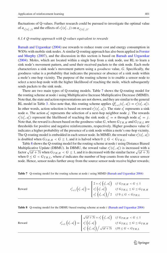
6.1.4 Q-routing approach with Q-values equivalent to rewards
Baruah and Urgaonkar (2004) use rewards to reduce route cost and energy consumption inWSNs with mobile sink nodes. A similar Q-routing approach has also been applied in Forsterand Murphy (2007), and the discussion in this section is based on Baruah and Urgaonkar(2004). Moles, which are located within a single hop from a sink node, use RL to learn asink node’s movement pattern, and send their received packets to the sink node. Each molecharacterizes a sink node’s movement pattern using a goodness value, G. Specifically, thegoodness value is a probability that indicates the presence or absence of a sink node withina mole’s one-hop vicinity. The purpose of the routing scheme is to enable a sensor node toselect a next-hop node with the higher likelihood of reaching the mole, which subsequentlysends packets to the sink node.
There are two main types of Q-routing models. Table 7 shows the Q-routing model forthe routing scheme at node i using Multiplicative Increase Multiplicative Decrease (MIMD).Note that, the state and action representations are not shown, and they are similar to the generalRL model in Table 3. Also note that, this routing scheme applies Qi
t+1(sit , ai
t ) = r it (s
it , ai
t ).In other words, action selection is based on reward r i
t (sit , ai
t ). The state sit represents a sink
node n. The action ait represents the selection of a next-hop neighbor node j . The rewards
r it (s
it , ai
t ) represent the likelihood of reaching the sink node sit = n through node ai
t = j .Note that, the reward is chosen based on the goodness value G, where GT H,H and GT H,L arethresholds for positive and negative reinforcements, respectively. Higher goodness value Gindicates a higher probability of the presence of a sink node within a mole’s one-hop vicinity.The Q-routing model is embedded in each sensor node. In MIMD, the reward value r i
t (sit , ai
t )
is doubled when GT H,H < G ≤ 1, and it is halved when 0 ≤ G < GT H,L .Table 8 shows the Q-routing model for the routing scheme at node i using Distance Biased
Multiplicative Update (DBMU). In DBMU, the reward value r it (s
it , ai
t ) is increased with afactor
√(d + 3) when GT H,H < G ≤ 1, and it is decreased with the similar factor
√(d + 3)
when 0 ≤ G < GT H,L , where d indicates the number of hop counts from the source sensornode. Hence, sensor nodes further away from the source sensor node receive higher rewards;
Table 7 Q-routing model for the routing scheme at node i using MIMD (Baruah and Urgaonkar 2004)
Reward r it+1
(sit , ai
t
)=
⎧⎪⎪⎪⎨⎪⎪⎪⎩
2× r it
(sit , ai
t
)i f GT H,H < G ≤ 1
r it
(sit , ai
t
)i f GT H,L ≤ G ≤ GT H,H
rit
(sit , ai
t
)/2 i f 0 ≤ G < GT H,L
Table 8 Q-routing model for the DBMU-based routing scheme at node i (Baruah and Urgaonkar 2004)
Reward r it+1
(sit , ai
t
)=
⎧⎪⎪⎪⎨⎪⎪⎪⎩
√(d + 3)× r i
t
(sit , ai
t
)i f GT H,H < G ≤ 1
r it
(sit , ai
t
)i f GT H,L ≤ G ≤ GT H,H
rit
(sit , ai
t
)/√(d + 3) i f 0 ≤ G < GT H,L
123
402 H. A. A. Al-Rawi et al.
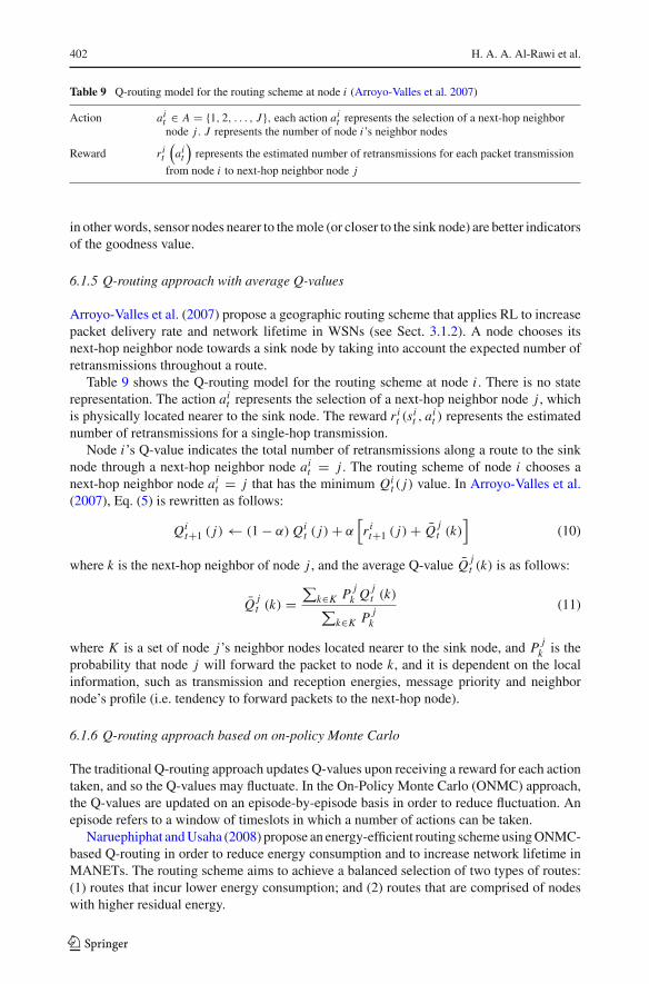
Table 9 Q-routing model for the routing scheme at node i (Arroyo-Valles et al. 2007)
Action ait ∈ A = {1, 2, . . . , J }, each action ai
t represents the selection of a next-hop neighbornode j . J represents the number of node i’s neighbor nodes
Reward r it
(ai
t
)represents the estimated number of retransmissions for each packet transmission
from node i to next-hop neighbor node j
in other words, sensor nodes nearer to the mole (or closer to the sink node) are better indicatorsof the goodness value.
6.1.5 Q-routing approach with average Q-values
Arroyo-Valles et al. (2007) propose a geographic routing scheme that applies RL to increasepacket delivery rate and network lifetime in WSNs (see Sect. 3.1.2). A node chooses itsnext-hop neighbor node towards a sink node by taking into account the expected number ofretransmissions throughout a route.
Table 9 shows the Q-routing model for the routing scheme at node i . There is no staterepresentation. The action ai
t represents the selection of a next-hop neighbor node j , whichis physically located nearer to the sink node. The reward r i
t (sit , ai
t ) represents the estimatednumber of retransmissions for a single-hop transmission.
Node i’s Q-value indicates the total number of retransmissions along a route to the sinknode through a next-hop neighbor node ai
t = j . The routing scheme of node i chooses anext-hop neighbor node ai
t = j that has the minimum Qit ( j) value. In Arroyo-Valles et al.
(2007), Eq. (5) is rewritten as follows:
Qit+1 ( j)← (1− α) Qi
t ( j)+ α[r i
t+1 ( j)+ Q̄ jt (k)
](10)
where k is the next-hop neighbor of node j , and the average Q-value Q̄ jt (k) is as follows:
Q̄ jt (k) =
∑k∈K P j
k Q jt (k)
∑k∈K P j
k
(11)
where K is a set of node j’s neighbor nodes located nearer to the sink node, and P jk is the
probability that node j will forward the packet to node k, and it is dependent on the localinformation, such as transmission and reception energies, message priority and neighbornode’s profile (i.e. tendency to forward packets to the next-hop node).
6.1.6 Q-routing approach based on on-policy Monte Carlo
The traditional Q-routing approach updates Q-values upon receiving a reward for each actiontaken, and so the Q-values may fluctuate. In the On-Policy Monte Carlo (ONMC) approach,the Q-values are updated on an episode-by-episode basis in order to reduce fluctuation. Anepisode refers to a window of timeslots in which a number of actions can be taken.
Naruephiphat and Usaha (2008) propose an energy-efficient routing scheme using ONMC-based Q-routing in order to reduce energy consumption and to increase network lifetime inMANETs. The routing scheme aims to achieve a balanced selection of two types of routes:(1) routes that incur lower energy consumption; and (2) routes that are comprised of nodeswith higher residual energy.
123
Application of reinforcement learning 403
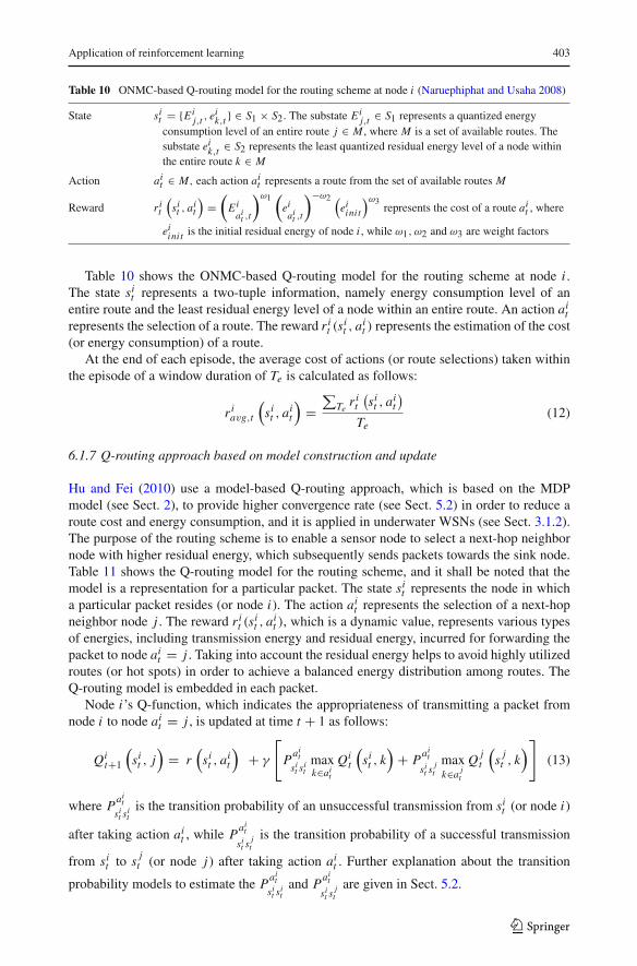
Table 10 ONMC-based Q-routing model for the routing scheme at node i (Naruephiphat and Usaha 2008)
State sit = {Ei
j,t , eik,t } ∈ S1 × S2. The substate Ei
j,t ∈ S1 represents a quantized energyconsumption level of an entire route j ∈ M , where M is a set of available routes. Thesubstate ei
k,t ∈ S2 represents the least quantized residual energy level of a node withinthe entire route k ∈ M
Action ait ∈ M, each action ai
t represents a route from the set of available routes M
Reward r it
(sit , ai
t
)=
(Ei
ait ,t
)ω1(
eiai
t ,t
)−ω2 (ei
ini t
)ω3represents the cost of a route ai
t , where
eiini t is the initial residual energy of node i , while ω1, ω2 and ω3 are weight factors
Table 10 shows the ONMC-based Q-routing model for the routing scheme at node i .The state si
t represents a two-tuple information, namely energy consumption level of anentire route and the least residual energy level of a node within an entire route. An action ai
trepresents the selection of a route. The reward r i
t (sit , ai
t ) represents the estimation of the cost(or energy consumption) of a route.
At the end of each episode, the average cost of actions (or route selections) taken withinthe episode of a window duration of Te is calculated as follows:
r iavg,t
(si
t , ait
)=
∑Te
r it
(si
t , ait
)
Te(12)
6.1.7 Q-routing approach based on model construction and update
Hu and Fei (2010) use a model-based Q-routing approach, which is based on the MDPmodel (see Sect. 2), to provide higher convergence rate (see Sect. 5.2) in order to reduce aroute cost and energy consumption, and it is applied in underwater WSNs (see Sect. 3.1.2).The purpose of the routing scheme is to enable a sensor node to select a next-hop neighbornode with higher residual energy, which subsequently sends packets towards the sink node.Table 11 shows the Q-routing model for the routing scheme, and it shall be noted that themodel is a representation for a particular packet. The state si
t represents the node in whicha particular packet resides (or node i). The action ai
t represents the selection of a next-hopneighbor node j . The reward r i
t (sit , ai
t ), which is a dynamic value, represents various typesof energies, including transmission energy and residual energy, incurred for forwarding thepacket to node ai
t = j . Taking into account the residual energy helps to avoid highly utilizedroutes (or hot spots) in order to achieve a balanced energy distribution among routes. TheQ-routing model is embedded in each packet.
Node i’s Q-function, which indicates the appropriateness of transmitting a packet fromnode i to node ai
t = j , is updated at time t + 1 as follows:
Qit+1
(si
t , j)= r
(si
t , ait
)+ γ
[P
ait
sit si
tmaxk∈ai
t
Qit
(si
t , k)+ P
ait
sit s j
tmaxk∈a j
t
Q jt
(s j
t , k)]
(13)
where Pai
t
sit si
tis the transition probability of an unsuccessful transmission from si
t (or node i)
after taking action ait , while P
ait
sit s j
tis the transition probability of a successful transmission
from sit to s j
t (or node j) after taking action ait . Further explanation about the transition
probability models to estimate the Pai
t
sit si
tand P
ait
sit s j
tare given in Sect. 5.2.
123
404 H. A. A. Al-Rawi et al.
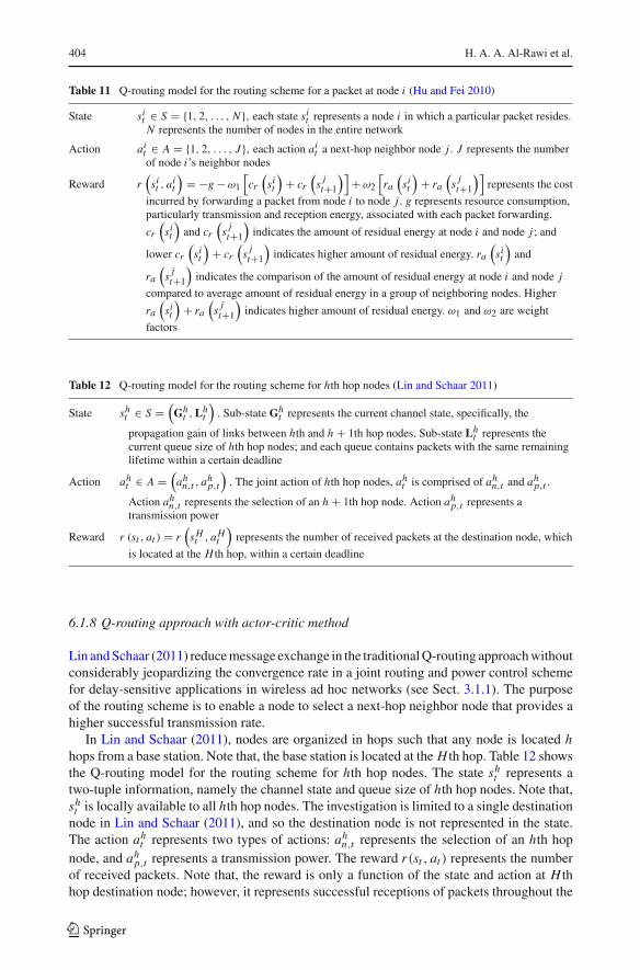
Table 11 Q-routing model for the routing scheme for a packet at node i (Hu and Fei 2010)
State sit ∈ S = {1, 2, . . . , N }, each state si
t represents a node i in which a particular packet resides.N represents the number of nodes in the entire network
Action ait ∈ A = {1, 2, . . . , J }, each action ai
t a next-hop neighbor node j . J represents the numberof node i’s neighbor nodes
Reward r(
sit , ai
t
)= −g−ω1
[cr
(sit
)+ cr
(s jt+1
)]+ω2
[ra
(sit
)+ ra
(s jt+1
)]represents the cost
incurred by forwarding a packet from node i to node j . g represents resource consumption,particularly transmission and reception energy, associated with each packet forwarding.
cr
(sit
)and cr
(s jt+1
)indicates the amount of residual energy at node i and node j ; and
lower cr
(sit
)+ cr
(s jt+1
)indicates higher amount of residual energy. ra
(sit
)and
ra
(s jt+1
)indicates the comparison of the amount of residual energy at node i and node j
compared to average amount of residual energy in a group of neighboring nodes. Higher
ra
(sit
)+ ra
(s jt+1
)indicates higher amount of residual energy. ω1 and ω2 are weight
factors
Table 12 Q-routing model for the routing scheme for hth hop nodes (Lin and Schaar 2011)
State sht ∈ S =
(Gh
t , Lht
). Sub-state Gh
t represents the current channel state, specifically, the
propagation gain of links between hth and h + 1th hop nodes. Sub-state Lht represents the
current queue size of hth hop nodes; and each queue contains packets with the same remaininglifetime within a certain deadline
Action aht ∈ A =
(ah
n,t , ahp,t
). The joint action of hth hop nodes, ah
t is comprised of ahn,t and ah
p,t .
Action ahn,t represents the selection of an h + 1th hop node. Action ah
p,t represents atransmission power
Reward r (st , at ) = r(
s Ht , aH
t
)represents the number of received packets at the destination node, which
is located at the H th hop, within a certain deadline
6.1.8 Q-routing approach with actor-critic method
Lin and Schaar (2011) reduce message exchange in the traditional Q-routing approach withoutconsiderably jeopardizing the convergence rate in a joint routing and power control schemefor delay-sensitive applications in wireless ad hoc networks (see Sect. 3.1.1). The purposeof the routing scheme is to enable a node to select a next-hop neighbor node that provides ahigher successful transmission rate.
In Lin and Schaar (2011), nodes are organized in hops such that any node is located hhops from a base station. Note that, the base station is located at the H th hop. Table 12 showsthe Q-routing model for the routing scheme for hth hop nodes. The state sh
t represents atwo-tuple information, namely the channel state and queue size of hth hop nodes. Note that,sh
t is locally available to all hth hop nodes. The investigation is limited to a single destinationnode in Lin and Schaar (2011), and so the destination node is not represented in the state.The action ah
t represents two types of actions: ahn,t represents the selection of an hth hop
node, and ahp,t represents a transmission power. The reward r(st , at ) represents the number
of received packets. Note that, the reward is only a function of the state and action at H thhop destination node; however, it represents successful receptions of packets throughout the
123
Application of reinforcement learning 405
entire network. Hence, r (st , at ) also indicates the successful transmission rate of all links inthe network.
Instead of using the traditional Q-routing-based Q-function (5), Lin and Schaar (2011)apply an actor-critic approach (Sutton and Barto 1998) in which the value function V h
t (sht ) (or
critic) and policy ρht (sh
t , aht ) (or actor) updates are separated. The critic is used to strengthen
or weaken the tendency of choosing a certain action, while the actor indicates the tendencyof choosing an action-state pair (Sutton and Barto 1998). Denote the difference in the valuefunction between hth hop (or the current hop) and h+ 1th hop (or the next hop) by δh
t (sht ) =
V h+1t (sh+1
t ) − V ht (sh
t ), the value function at hth hop nodes is updated using V ht+1(s
ht+1) =
(1− α)V ht (sh
t )+α[δht (sh
t )], and so it is updated using value functions received from h+1thhop nodes. Denote δH
t (s Ht ) = r(st , at ) + γ Vt (st ) − V H
t (s Ht ), the value function at H th
hop nodes (or the destination node) is V Ht+1(s
Ht+1) = (1− α)V H
t (s Ht ) + α[δH
t (s Ht )], and so
it is updated using value function Vt (st ), which is received from 1th hop nodes (or all thesource nodes), and reward r(st , at ). Therefore, the reward r(st , at ) is distributed throughoutthe network in the form of value function V h
t (sht ). The routing scheme of an hth hop node
chooses a next-hop neighbor node and transmission power aht that provide the maximum
ρht (sh
t , aht ) value, which is updated by ρh
t+1(sht+1, ah
t+1) = ρht (sh
t , aht ) + βδh
t (sht ), where β
is the learning rate. This routing scheme has been shown to increase the number of receivedpackets at the destination node within a certain deadline (or goodput).
Lin and Schaar (2011) also propose two approaches to reduce message exchange. Firstly,only a subset of nodes within an hth hop is involved in estimating the value function V h
t
(sh
t
).
Secondly, message exchanges are only carried out after a certain number of time slots.
6.2 Multi-agent reinforcement learning (MARL) model
Multi-Agent Reinforcement Learning (MARL) model decomposes a system-wide optimiza-tion problem into sets of local optimization problems, which are solved through collaborationwithout using global information. The collaboration may take the form of exchanging localinformation including knowledge (i.e Q-value), observations (or states) and decisions (oractions). For instance, MARL enables a node to collaborate with its neighbor nodes, andsubsequently make local decisions independently in order to achieve network performanceenhancement.
6.2.1 MARL approach with reward exchange
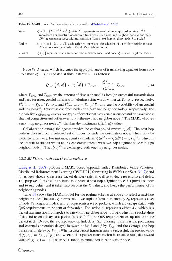
Elwhishi et al. (2010) propose a MARL-based routing scheme for delay tolerant networks(see Sect. 3.1.4), and it has been shown to increase packet delivery rate, as well as to decreasetransmission delay. Routing schemes for delay tolerant networks are characterized by thelack of end-to-end aspect, and each node explores network connectivity through finding anew link to a next-hop neighbor node when a new packet arrives, which must be kept inthe buffer while a link is formed. The purpose of this routing scheme is to select a reliablenext-hop neighbor node, and it takes into account three main factors. Specifically, two factorsthat are relevant to the channel availability (node mobility and congestion level) and a singlefactor that is relevant to the buffer utilization (remaining space in the buffer).
Table 13 shows the MARL model for node i to select a reliable next-hop neighbor node.The state si
t includes three events {Bi , Ui, j , D j,i }. The action ait represents a transmission
from node i to a next-hop neighbor node j . The reward represents the amount of time inwhich a mobile node i and a node j are neighbor nodes. The MARL model is embedded ineach node.
123
406 H. A. A. Al-Rawi et al.
Table 13 MARL model for the routing scheme at node i (Elwhishi et al. 2010)
State sit ∈ S = {Bi , Ui, j , D j,i }, state Bi represents an event of nonempty buffer; state Ui, j
represents a successful transmission from node i to a next-hop neighbor node j ; and stateD j,i represents a successful transmission from a next-hop neighbor node j to node i
Action ait ∈ A = {1, 2, . . . , J }, each action ai
t represents the selection of a next-hop neighbor nodej . J represents the number of node i’s neighbor nodes
Reward r it
(ai
t
)represents the amount of time in which node i and node ai
t = j are neighbor nodes
Node i’s Q-value, which indicates the appropriateness of transmitting a packet from nodei to a node ai
t = j , is updated at time instant t + 1 as follows:
Qit+1
(si
t , ait
)← r i
t
(ai
t
)+ T f ree − Pi, j
unsuccess
Pi, jsuccess
Tbusy (14)
where T f ree and Tbusy are the amount of time a channel is free (or successful transmission)and busy (or unsuccessful transmission) during a time window interval Twindow, respectively;Pi, j
success = T f ree/Twindow and Pi, junsuccess = Tbusy/Twindow are the probability of successful
and unsuccessful transmissions from node i to a next-hop neighbor node j , respectively. Theprobability Pi, j
unsuccess covers two types of events that may cause unsuccessful transmissions:channel congestion and buffer overflow at the next-hop neighbor node j . The MARL choosesa next-hop neighbor node ai, j
j that has the maximum Qit (s
it , ai
t ) value.
Collaboration among the agents involve the exchanges of reward r it (a
it ). The next-hop
node is chosen from a selected set of nodes towards the destination node, which may bemultiple hops away. For instance, agent i calculates r i
t (ai,kt ) = r i
t (ai, jt )+ r j
t (a j,kt ), which is
the amount of time in which node i can communicate with two-hop neighbor node k thoughneighbor node j . The r i
t (ai,kt ) is exchanged with one-hop neighbor nodes.
6.2.2 MARL approach with Q-value exchange
Liang et al. (2008) propose a MARL-based approach called Distributed Value Function-Distributed Reinforcement Learning (DVF-DRL) for routing in WSNs (see Sect. 3.1.2); andit has been shown to increase packet delivery rate, as well as to decrease end-to-end delay.The purpose of this routing scheme is to select a next-hop neighbor node that provides lowerend-to-end delay; and it takes into account the Q-values, and hence the performance, of itsneighboring nodes.
Table 14 shows the MARL model for the routing scheme at node i to select a next-hopneighbor node. The state si
t represents a two-tuple information, namely Sn represents a setof node i’s neighbor nodes, and Sp represents a set of packets, which are encapsulated withQoS requirements, to be sent or forwarded. The action ai
t represents either A f , which is apacket transmission from node i to a next-hop neighbor node j ; or Ad , which is a packet dropif the end-to-end delay of a packet fails to fulfill the QoS requirement encapsulated in thepacket itself. Denote the average one-hop link delay (i.e. queuing, transmission, processingand channel contention delays) between nodes i and j by TPi j , and the average one-hoptransmission delay by TPavr . When a data packet transmission is successful, the reward valuer i
t (sit , ai
t ) = TPavr /TPi j ; and when a data packet transmission is unsuccessful, the rewardvalue r i
t (sit , ai
t ) = −1. The MARL model is embedded in each sensor node.
123
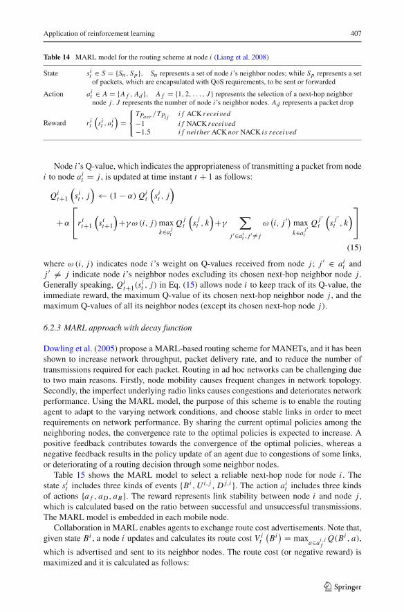
Application of reinforcement learning 407
Table 14 MARL model for the routing scheme at node i (Liang et al. 2008)
State sit ∈ S = {Sn , Sp}, Sn represents a set of node i’s neighbor nodes; while Sp represents a setof packets, which are encapsulated with QoS requirements, to be sent or forwarded
Action ait ∈ A = {A f , Ad }, A f = {1, 2, . . . , J } represents the selection of a next-hop neighbornode j . J represents the number of node i’s neighbor nodes. Ad represents a packet drop
Reward r it
(sit , ai
t
)=
⎧⎨⎩
TPavr /TPi j i f ACK received−1 i f NACK received−1.5 i f nei ther ACK nor NACK is received
Node i’s Q-value, which indicates the appropriateness of transmitting a packet from nodei to node ai
t = j , is updated at time instant t + 1 as follows:
Qit+1
(si
t , j)← (1− α) Qi
t
(si
t , j)
+α
⎡⎣r i
t+1
(si
t+1
)+γω (i, j) max
k∈a jt
Q jt
(s j
t , k)+γ
∑
j ′∈ait , j ′ �= j
ω(i, j ′
)maxk∈a j ′
t
Q j ′t
(s j ′
t , k)⎤⎦
(15)
where ω (i, j) indicates node i’s weight on Q-values received from node j ; j ′ ∈ ait and
j ′ �= j indicate node i’s neighbor nodes excluding its chosen next-hop neighbor node j .Generally speaking, Qi
t+1(sit , j) in Eq. (15) allows node i to keep track of its Q-value, the
immediate reward, the maximum Q-value of its chosen next-hop neighbor node j , and themaximum Q-values of all its neighbor nodes (except its chosen next-hop node j).
6.2.3 MARL approach with decay function
Dowling et al. (2005) propose a MARL-based routing scheme for MANETs, and it has beenshown to increase network throughput, packet delivery rate, and to reduce the number oftransmissions required for each packet. Routing in ad hoc networks can be challenging dueto two main reasons. Firstly, node mobility causes frequent changes in network topology.Secondly, the imperfect underlying radio links causes congestions and deteriorates networkperformance. Using the MARL model, the purpose of this scheme is to enable the routingagent to adapt to the varying network conditions, and choose stable links in order to meetrequirements on network performance. By sharing the current optimal policies among theneighboring nodes, the convergence rate to the optimal policies is expected to increase. Apositive feedback contributes towards the convergence of the optimal policies, whereas anegative feedback results in the policy update of an agent due to congestions of some links,or deteriorating of a routing decision through some neighbor nodes.
Table 15 shows the MARL model to select a reliable next-hop node for node i . Thestate si
t includes three kinds of events {Bi , Ui, j , D j,i }. The action ait includes three kinds
of actions {a f , aD, aB}. The reward represents link stability between node i and node j ,which is calculated based on the ratio between successful and unsuccessful transmissions.The MARL model is embedded in each mobile node.
Collaboration in MARL enables agents to exchange route cost advertisements. Note that,given state Bi , a node i updates and calculates its route cost V i
t
(Bi
) = maxa∈ai, j
fQ(Bi , a),
which is advertised and sent to its neighbor nodes. The route cost (or negative reward) ismaximized and it is calculated as follows:
123
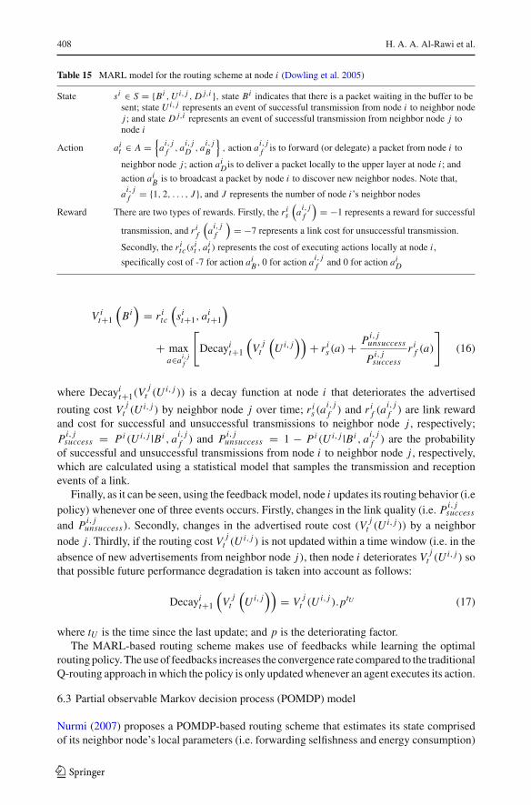
408 H. A. A. Al-Rawi et al.
Table 15 MARL model for the routing scheme at node i (Dowling et al. 2005)
State si ∈ S = {Bi , Ui, j , D j,i }, state Bi indicates that there is a packet waiting in the buffer to besent; state Ui, j represents an event of successful transmission from node i to neighbor nodej ; and state D j,i represents an event of successful transmission from neighbor node j tonode i
Action ait ∈ A =
{ai, j
f , ai, jD , ai, j
B
}, action ai, j
f is to forward (or delegate) a packet from node i to
neighbor node j ; action aiD is to deliver a packet locally to the upper layer at node i ; and
action aiB is to broadcast a packet by node i to discover new neighbor nodes. Note that,
ai, jf = {1, 2, . . . , J }, and J represents the number of node i’s neighbor nodes
Reward There are two types of rewards. Firstly, the r is
(ai, j
f
)= −1 represents a reward for successful
transmission, and r if
(ai, j
f
)= −7 represents a link cost for unsuccessful transmission.
Secondly, the r itc(s
it , ai
t ) represents the cost of executing actions locally at node i ,
specifically cost of -7 for action aiB , 0 for action ai, j
f and 0 for action aiD
V it+1
(Bi
)= r i
tc
(si
t+1, ait+1
)
+ maxa∈ai, j
f
[Decayi
t+1
(V j
t
(Ui, j
))+ r i
s (a)+ Pi, junsuccess
Pi, jsuccess
r if (a)
](16)
where Decayit+1(V j
t (Ui, j )) is a decay function at node i that deteriorates the advertised
routing cost V jt (Ui, j ) by neighbor node j over time; r i
s (ai, jf ) and r i
f (ai, jf ) are link reward
and cost for successful and unsuccessful transmissions to neighbor node j , respectively;Pi, j
success = Pi (Ui, j |Bi , ai, jf ) and Pi, j
unsuccess = 1 − Pi (Ui, j |Bi , ai, jf ) are the probability
of successful and unsuccessful transmissions from node i to neighbor node j , respectively,which are calculated using a statistical model that samples the transmission and receptionevents of a link.
Finally, as it can be seen, using the feedback model, node i updates its routing behavior (i.epolicy) whenever one of three events occurs. Firstly, changes in the link quality (i.e. Pi, j
success
and Pi, junsuccess). Secondly, changes in the advertised route cost (V j
t (Ui, j )) by a neighbornode j . Thirdly, if the routing cost V j
t (Ui, j ) is not updated within a time window (i.e. in theabsence of new advertisements from neighbor node j), then node i deteriorates V j
t (Ui, j ) sothat possible future performance degradation is taken into account as follows:
Decayit+1
(V j
t
(Ui, j
))= V j
t (Ui, j ).ptU (17)
where tU is the time since the last update; and p is the deteriorating factor.The MARL-based routing scheme makes use of feedbacks while learning the optimal
routing policy. The use of feedbacks increases the convergence rate compared to the traditionalQ-routing approach in which the policy is only updated whenever an agent executes its action.
6.3 Partial observable Markov decision process (POMDP) model
Nurmi (2007) proposes a POMDP-based routing scheme that estimates its state comprisedof its neighbor node’s local parameters (i.e. forwarding selfishness and energy consumption)
123
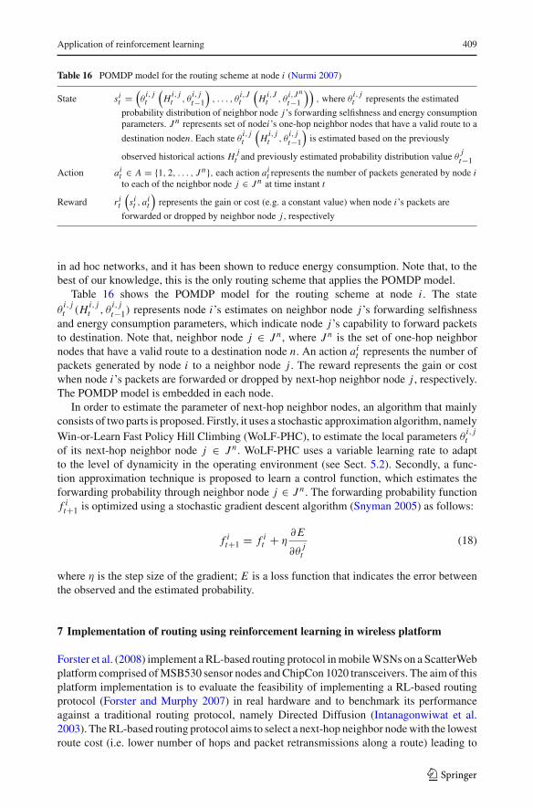
Application of reinforcement learning 409
Table 16 POMDP model for the routing scheme at node i (Nurmi 2007)
State sit =
(θ
i, jt
(Hi, j
t , θi, jt−1
), . . . , θ
i,Jt
(Hi,J
t , θi,J n
t−1
)), where θ
i, jt represents the estimated
probability distribution of neighbor node j’s forwarding selfishness and energy consumptionparameters. J n represents set of nodei’s one-hop neighbor nodes that have a valid route to a
destination noden. Each state θi, jt
(Hi, j
t , θi, jt−1
)is estimated based on the previously
observed historical actions H jt and previously estimated probability distribution value θ
jt−1
Action ait ∈ A = {1, 2, . . . , J n}, each action ai
t represents the number of packets generated by node ito each of the neighbor node j ∈ J n at time instant t
Reward r it
(sit , ai
t
)represents the gain or cost (e.g. a constant value) when node i’s packets are
forwarded or dropped by neighbor node j , respectively
in ad hoc networks, and it has been shown to reduce energy consumption. Note that, to thebest of our knowledge, this is the only routing scheme that applies the POMDP model.
Table 16 shows the POMDP model for the routing scheme at node i . The stateθ
i, jt (Hi, j
t , θi, jt−1) represents node i’s estimates on neighbor node j’s forwarding selfishness
and energy consumption parameters, which indicate node j’s capability to forward packetsto destination. Note that, neighbor node j ∈ J n , where J n is the set of one-hop neighbornodes that have a valid route to a destination node n. An action ai
t represents the number ofpackets generated by node i to a neighbor node j . The reward represents the gain or costwhen node i’s packets are forwarded or dropped by next-hop neighbor node j , respectively.The POMDP model is embedded in each node.
In order to estimate the parameter of next-hop neighbor nodes, an algorithm that mainlyconsists of two parts is proposed. Firstly, it uses a stochastic approximation algorithm, namelyWin-or-Learn Fast Policy Hill Climbing (WoLF-PHC), to estimate the local parameters θ
i, jt
of its next-hop neighbor node j ∈ J n . WoLF-PHC uses a variable learning rate to adaptto the level of dynamicity in the operating environment (see Sect. 5.2). Secondly, a func-tion approximation technique is proposed to learn a control function, which estimates theforwarding probability through neighbor node j ∈ J n . The forwarding probability functionf it+1 is optimized using a stochastic gradient descent algorithm (Snyman 2005) as follows:
f it+1 = f i
t + η∂ E
∂θj
t
(18)
where η is the step size of the gradient; E is a loss function that indicates the error betweenthe observed and the estimated probability.
7 Implementation of routing using reinforcement learning in wireless platform
Forster et al. (2008) implement a RL-based routing protocol in mobile WSNs on a ScatterWebplatform comprised of MSB530 sensor nodes and ChipCon 1020 transceivers. The aim of thisplatform implementation is to evaluate the feasibility of implementing a RL-based routingprotocol (Forster and Murphy 2007) in real hardware and to benchmark its performanceagainst a traditional routing protocol, namely Directed Diffusion (Intanagonwiwat et al.2003). The RL-based routing protocol aims to select a next-hop neighbor node with the lowestroute cost (i.e. lower number of hops and packet retransmissions along a route) leading to
123
410 H. A. A. Al-Rawi et al.
multiple sink nodes (Forster and Murphy 2007). Additionally, a random backoff delay wasintroduced to reduce channel contention.
Compared to the traditional Directed Diffusion (Intanagonwiwat et al. 2003) routing pro-tocol, the findings of the platform implementation is that, the RL-based routing protocol:
• Provides lower routing cost.• Provides higher packet delivery rate or lower packet loss rate attributed to the optimal
routes.• Requires higher memory requirement due to the complex data structures required to store
the Q-values.• Causes higher route discovery delay.
8 Performance enhancements
Table 17 shows the performance enhancements brought about by the application of RLin various routing schemes. The RL approach has been shown to achieve the followingperformance enhancements.
a. Lower end-to-end delay.b. Higher throughput.c. Higher packet delivery rate or lower packet loss rate.d. Lower routing overhead. Lower routing overhead may indicate more stable routes (or
higher route robustness), and so it may indicate a lower number of packet retransmissions(Dowling et al. 2005). Usaha (2004) reduces the number of route discovery messagesby incorporating a cache, which stores routing information, at each mobile node. Thisreduces the need to invoke the route discovery process for each connection request.
e. Longer network lifetime. Longer network lifetime indicates lower energy consumption.For instance, Nurmi (2007) takes account of the residual energy of each node in routingin order to increase network lifetime.
f. Higher reward value. Bhorkar et al. (2012) achieves higher reward value, which indicateslower average cost incurred by routing.
9 Open issues
This section discusses open issues that can be pursued in this area. Additionally, furtherresearch could be pursued to investigate the new features discussed in Sect. 5.
9.1 Suitability and comparisons of action selection approaches
Action selection techniques, such as ε -greedy and softmax (see Sect. 2.2) have been widelyapplied in the literature. The ε-greedy approach performs exploration with small probabilityε (e.g. ε = 0.1), and exploitation with probability 1 − ε. On the other hand, the softmaxapproach ranks the exploration actions so that it does not explore actions that are far awayfrom the optimal action. Nevertheless, each action selection technique has its merits anddemerits in regards to the respective applications. Hence, further research could be pursuedto investigate the suitability and network performance brought about by each of the techniquesfor routing in distributed wireless networks.
123
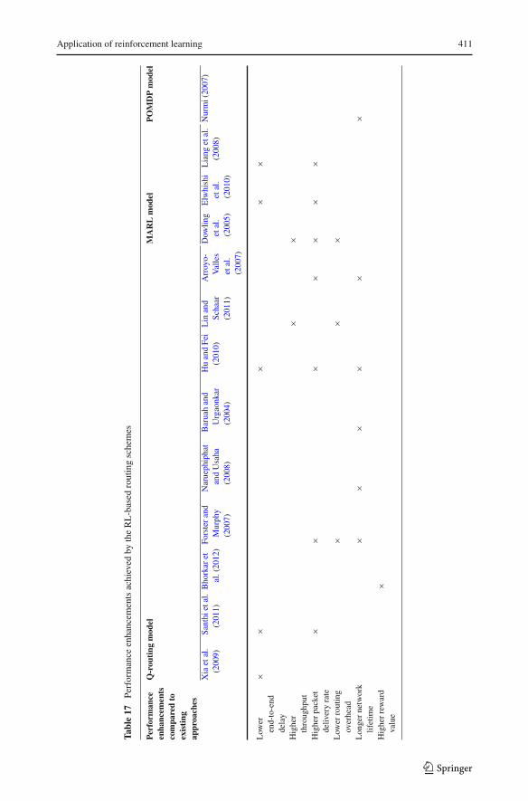
Application of reinforcement learning 411
Tabl
e17
Perf
orm
ance
enha
ncem
ents
achi
eved
byth
eR
L-b
ased
rout
ing
sche
mes
Per
form
ance
enha
ncem
ents
com
pare
dto
exis
ting
appr
oach
es
Q-r
outi
ngm
odel
MA
RL
mod
elP
OM
DP
mod
el
Xia
etal
.(2
009)
Sant
hiet
al.
(201
1)B
hork
aret
al.(
2012
)Fo
rste
ran
dM
urph
y(2
007)
Nar
ueph
ipha
tan
dU
saha
(200
8)
Bar
uah
and
Urg
aonk
ar(2
004)
Hu
and
Fei
(201
0)L
inan
dSc
haar
(201
1)
Arr
oyo-
Val
les
etal
.(2
007)
Dow
ling
etal
.(2
005)
Elw
hish
iet
al.
(201
0)
Lia
nget
al.
(200
8)N
urm
i(20
07)
Low
eren
d-to
-end
dela
y
××
××
×
Hig
her
thro
ughp
ut×
×
Hig
her
pack
etde
liver
yra
te×
××
××
××
Low
erro
utin
gov
erhe
ad×
××
Lon
ger
netw
ork
lifet
ime
××
××
××
Hig
her
rew
ard
valu
e×
123
412 H. A. A. Al-Rawi et al.
9.2 Degradation of optimal route due to exploitation
Exploitation may deliver all data packets along the same optimal (or near-optimal) route,which may cause congestion, resulting in higher energy consumption, routing overhead, aswell as the degradation of network performance. Various traditional approaches may be usedto ameliorate this issue as described below:
• Increasing learning rate. This increases the responsiveness of nodes to the dynamic con-ditions of the operating environment. When an optimal route becomes congested, nodesmay change their respective routes. However, a new route may be suboptimal comparedto the existing one. For instance, some intermediate nodes may have lower residualenergy. Hence, achieving a better balance in energy consumption among various routes,including the optimal route, is necessary.• Increasing exploration rate. This reduces the traffic load on the optimal route. Never-
theless, this may affect the network performance because the traditional explorationtechniques may choose the non-optimal routes, which may not meet the requirements onnetwork performance.• Using different QoS classes. This enables nodes to achieve a balance among the avail-
able routes based on the QoS requirements. For instance, high priority traffics may usean optimal route (i.e exploitation), while lower priority traffics may use a suboptimalroute (i.e exploration). For instance, Fu et al. (2005) adopt a genetic-based approach forexploration in route discovery, in which routes are discovered based on a predefined setof QoS goals (e.g. the throughput and end-to-end delay requirements). This approach hasbeen shown to improve the network performance. Further research could be pursued toinvestigate the effectiveness and amount of overhead of this technique, the coordinationamong nodes for QoS provisioning along a route, as well as to ameliorate the selfishnessof intermediate nodes.
9.3 Multi-agent RL approaches
Most routing schemes in the literature have been applying the traditional single-agent RLapproach. These schemes have been shown to improve network performance. Nevertheless,the performance may be further enhanced using the multi-agent RL model (see Sect. 4.2)(Dowling et al. 2005; Elwhishi et al. 2010; Liang et al. 2008). The multi-agent RL modelaims to coordinate agents in order to achieve the optimal network-wide performance, andits application in the literature has been limited. Nevertheless, the multi-agent RL approachrequires additional overhead and complexity (Di Felice et al. 2010; Dowling et al. 2005),and so further research could be pursued to address these issues. In regards to the challengesof each type of distributed wireless network (see Table 1), some of the expected advantagesbrought about by coordination through the application of multi-agent RL approach are asfollows:
• Mobile Ad Hoc Networks (see Sect. 3.1.1). The application of multi-agent RL approachmay improve the coordination of nodes moving in groups, which may be an importantfactor in nodes’ routing decisions. Consequently, the routing decision of nodes in eachgroup can be further enhanced and coordinated in real-time.• Wireless Sensor Networks (see Sect. 3.1.2). The application of the multi-agent RL
approach may prolong network lifetime of a WSN. For instance, the neighboring sensornodes may cooperate with each other to choose a sensor node with higher residual energyas clusterhead so that it is capable of collecting and forwarding data to the sink node.
123
Application of reinforcement learning 413
• Cognitive Radio Networks (see Sect. 3.1.3). The application of multi-agent RL approachmay be helpful to solve many issues that require coordination among SUs, as well asPUs. For instance, the neighboring SUs can share their respective estimations of PUutilization level, which is location-dependent. Subsequently, they can coordinate theirrespective routing decisions in order to reduce the interference to PUs.• Delay Tolerant Networks (see Sect. 3.1.4). The application of multi-agent RL has been
shown to improve the network-wide performance. For instance, Elwhishi et al. (2010)propose a MARL-based routing scheme that enables neighboring nodes to collaborateamong themselves so that they can respectively select a reliable next-hop based on threefactors, namely node mobility, the congestion level, and the buffer utilization level.
9.4 Exploration with stability enhancement
Exploration helps a routing scheme to converge to an optimal route selection policy. However,route discovery using non-optimal actions may increase network instability. Consequently,network performance (e.g. throughput and end-to-end delay) may fluctuate. While variousapproaches have been proposed to provide a balanced tradeoff between exploitation andexploration, further research could be pursued to investigate the possibility of achieving routeexploration, while minimizing network instability. For instance, using rules, exploration maybe triggered based on the required network performance level. Exploration of non-optimalroutes may only be granted if network performance is unsatisfactory.
9.5 Application of events to routing
Another feature that can be incorporated into the traditional RL-based routing scheme iscalled event. Traditionally, state monitors the conditions of the operating environment at alltimes. In contrast, event, such as node failure and handoff, is detected occasionally wheneverit occurs (Yau et al. 2012). In a highly dynamic operating environment, Q-values may changerapidly and fluctuate. The event may capture and detect the fluctuation of Q-values so thatappropriate actions can be taken in order to improve the convergence rate and networkperformance.
Rules (see Sect. 5.5) and events may be also applied together. For instance, rules andevents can improve the estimation of Q-values, and avoid invalid routes. For example, whenmobile nodes move out of range, their respective Q-values may become invalid, and so mak-ing routing decisions based on these Q-values may degrade the network performance. Anevent may be applied to detect whether a node is out-of-range due to node movement; subse-quently rules may be applied to set Q-values of neighbor nodes to infinity (Yau et al. 2012;Chang et al. 2004).
9.6 Lack of the implementation of RL-based routing schemes on wireless platform
To the best of our knowledge, there is only a single implementation of RL-based routingscheme in wireless platform by Forster et al. (2008) (see Sect. 7), and most of the existingrouting schemes have been evaluated using simulation. Real implementation on wirelessplatform is important to validate the correctness and feasibility of RL-based schemes. Furtherresearch can be pursued to investigate the implementation and challenges of the RL-basedrouting schemes on wireless platforms.
123
414 H. A. A. Al-Rawi et al.
10 Conclusions
Reinforcement Learning (RL) has been applied to various routing schemes for distributedwireless networks, including wireless ad hoc networks, wireless sensor networks, cognitiveradio networks and delay tolerant networks, and it has been shown to improve networkperformance, such as higher throughput and lower end-to-end delay. RL enables a wirelessnode to observe its local operating environment, and subsequently learn to make globalrouting decisions efficiently. The advantages brought about by RL to routing are foreseen todraw significant research interests in the near future. This article has provided an extensivereview on the existing RL-based routing schemes in distributed wireless networks. Firstly,this article presents Q-learning, which is a popular RL approach. Secondly, it identifiesthe challenges and advantages brought about by RL in various types of distributed wirelessnetworks. A general RL model for routing is also presented. Thirdly, it presents three types ofRL models for routing, namely Q-routing, multi-agent RL, and partially observable Markovdecision process. Fourthly, it provides an extensive review on how various routing schemeshave been formulated and modeled using RL in order to improve network performance.Fifthly, new features aiming to enhance the traditional RL approach for routing are presented.Sixthly, it presents an implementation of RL-based routing scheme on wireless platform.Seventhly, it presents performance enhancements achieved by the RL-based routing schemes.Lastly, it discusses the open issues associated with the application of RL in the routingschemes. Certainly, there is a substantial room for future work in the application of RL torouting.
References
Akyildiz IF, Su W, Sankarasubramaniam Y, Cayirci E (2002) Wireless sensor networks: a survey. ComputNetw 38(4):393–422
Akyildiz IF, Lee WY, Chowdhury KR (2009) Cognitive radio ad hoc networks. Ad Hoc Netw 7(5):810–836Al-Rawi HAA, Yau K-LA (2012) Routing in distributed cognitive radio networks: a survey. Wirel Pers Com-
mun Int J. doi:10.1007/s11277-012-0674-7Albus JS (1975) A new approach to manipulator control: the cerebellar model articulation controller. J Dyn
Syst Meas Control 97:220–227Arroyo-Valles R, Alaiz-Rodriquez R, Guerrero-Curieses A, Cid-Sueiro J (2007) Q-probabilistic routing in
wireless sensor networks. In: Proceedings of ISSNIP 3rd international conference intelligent sensors,sensor network and information processing, pp. 1–6
Baruah P, Urgaonkar R (2004) Learning-enforced time domain routing to mobile sinks in wireless sensorfields. In: Proceedings of LCN 29th annals IEEE international conference local computer networks, pp.525–532
Bhorkar AA, Naghshvar M, Javidi T, Rao BD (2012) Adaptive opportunistic routing for wireless ad hocnetworks. IEEE ACM Trans Netw 20(1):243–256
Boyan J, Littman ML (1994) Packet routing in dynamically changing networks: a reinforcement learningapproach. In: Proceedings of NIPS Adv neural information processing systems, pp 671–678
Boukerche A (2009) Algorithms and protocols for wireless, mobile and ad hoc networks. Wiley, New JerseyBurleigh S, Hooke A, Torgerson L, Fall K, Cerf V, Durst B, Scott K, Weiss H (2003) Delay-tolerant networking:
an approach to interplanetary internet. IEEE Commun Mag 41(6):128–136Bowling M, Veloso M (2002) Multiagent learning using a variable learning rate. Artif Intell 136(2):215–250Chang Y-H, Ho T, Kaelbling LP (2004) Mobilized ad-hoc networks: a reinforcement learning approach. In:
Proceedings of ICAC international conference autonomic computer, pp 240–247Chetret D, Tham C-K, Wong LWC (2004) Reinforcement learning and CMAC-based adaptive routing for
MANETs. In: Proceedings of ICON 12th IEEE international conference networks, pp. 540–544Clausen T, Jacquet P (2003) Optimized link state routing protocol (OLSR). IETF RFC 3626Dearden R, Friedman N, Andre D (1999) Model based Bayesian exploration. In: Proceedings of UAI 15th
conference uncertainty, artificial intelligence, pp 150–159
123
Application of reinforcement learning 415
Di Felice M, Chowdhury KR, Wu C, Bononi L, Meleis W (2010) Learning-based spectrum selection incognitive radio ad hoc networks. In: Proceedings of WWIC 8th international conference wired wirelessinternet communications, pp 133–145
Dong S, Agrawal P, Sivalingam K (2007) Reinforcement learning based geographic routing protocol for UWBwireless sensor network. In: Proceedings of GLOBECOM IEEE global telecommunications conference,pp 652–656
Dowling J, Curran E, Cunningham R, Cahill V (2005) Using feedback in collaborative reinforcement learningto adaptively optimize MANET routing. IEEE Trans Syst Man Cybern Part A Syst Hum 35(3):360–372
Elwhishi A, Ho P-H, Naik K, Shihada B (2010) ARBR: Adaptive reinforcement-based routing for DTN. In:Proceedings of WIMOB IEEE 6th international conference wireless and mobile computes, networks andcommunications, pp. 376–385
Forster A (2007) Machine learning techniques applied to wireless ad-hoc networks: guide and survey. In:Proceedings of ISSNIP 3rd international conference intelligent sensors, sensor Networks and information,pp. 365–370
Forster A, Murphy AL (2007) FROMS: Feedback routing for optimizing multiple sinks in WSN with rein-forcement learning. In: Proceedings of ISSNIP 3rd international conference intelligent sensors, sensorNetworks and, informations, pp. 371–376
Forster A, Murphy AL, Schiller J, Terfloth K (2008) An efficient implementation of reinforcement learningbased routing on real WSN hardware. In: Proceedings of WIMOB IEEE international conference wirelessand mobile computers, networks and communcations, pp 247–252
Fu P, Li J, Zhang D (2005) Heuristic and distributed QoS route discovery for mobile ad hoc networks. In:Proceedings of the CIT 5th international conference on computer and information technology, pp. 512–516
Gen M, Cheng R (1999) Genetic algorithms and engineering optimization. Wiley, NYHao S, Wang T (2006) Sensor networks routing via Bayesian exploration. In: Proceedings of LCN 31th annals
of IEEE international conference local computing Networks, pp. 954–955Hu T, Fei Y (2010) QELAR: a machine-learning-based adaptive routing protocol for energy-efficient and
lifetime-extended underwater sensor networks. IEEE Trans Mobile Comput 9(6):796–809Intanagonwiwat C, Govindan R, Estrin D, Heidemann J, Silva F (2003) Directed diffusion for wireless sensor
networking. IEEE ACM Trans Netw 11(1):2–16Kennedy J, Eberhart R (1995) Particle swarm optimization. In: Proceedings of IEEE international conference
neural networks. pp 1942–1948Kumar S, Miikkulainen R (1997) Dual reinforcement Q-routing: an on-line adaptive routing algorithm. In:
Proceedings of ANNIE artificial neural networks in engineering conference. pp 231–238Liang X, Balasingham I, Byun S-S (2008) A multi-agent reinforcement learning based routing protocol for
wireless sensor networks. In: Proceedings of ISWCS IEEE international symposium Wireless communi-cations systems. pp 552–557
Lin Z, Schaar Mvd (2011) Autonomic and distributed joint routing and power control for delay-sensitiveapplications in multi-hop wireless networks. IEEE Tran Wirel Commun 10(1):102–113
Naruephiphat W, Usaha W (2008) Balancing tradeoffs for energy-efficient routing MANETs based on rein-forcement learning. In: Proceedings of VTC spring IEEE vehicular techmology conference. pp 2361–2365
Nurmi P (2007) Reinforcement learning for routing in ad hoc networks. In: Proceedings of WiOpt 5th inter-national symposium modeling and optimization in mobile, ad hoc and wireless network and workshops,pp 1–8
Ouzecki D, Jevtic D (2010) Reinforcement learning as adaptive network routing of mobile agents. In: Pro-ceedings of MIPRO 33rd international convention, pp 479–484
Perkins CE, Royer EM (1999) Ad-hoc on-demand distance vector routing. In: Proceedings of WMCSA mobilecomputers systems and applications, pp 90–100
Rojas R (1996) Neural networks: a systematic introduction. Springer, NYSanthi G, Nachiappan A, Ibrahime MZ, Raghunadhane R, Favas MK (2011) Q-learning based adaptive QoS
routing protocol for MANETs. In: Proceedings of ICRTIT international conference recent trends in infor-mation technology, pp 1233–1238
Sutton RS, Barto AG (1998) Reinforcement learning: an introduction. MIT Press, CambridgeSnyman A (2005) Practical mathematical optimization: an introduction to basic optimization theory and
classical and new gradient-based algorithms. Springer, NYToh CK (2001) Ad hoc mobile wireless networks: protocols and systems. Prentice Hall, New JerseyUsaha W (2004) A reinforcement learning approach for path discovery in MANETs with path caching strategy.
In: Proceedings of ISWCS 1st international symposium wireless communications systems, pp 220–224Xia B, Wahab MH, Yang Y, Fan Z, Sooriyabandara M (2009) Reinforcement learning based spectrum-aware
routing in multi-hop cognitive radio networks. In: Proceedings of CROWNCOM 4th international confer-ence cognitive radio oriented wireless networks and communications, pp 1–5
123
416 H. A. A. Al-Rawi et al.
Yau K-LA, Komisarczuk P, Teal PD (2012) Reinforcement learning for context awareness and intelligence inwireless networks: review, new features and open issues. J Netw Comput Appl 35(1):253–267
Yin GG, Krishnamurthy V (2005) Least mean square algorithms with markov regime-switching limit. IEEETrans Autom Control 50(5):577–593
Yu FR, Wong VWS, Leong VCM (2008) A new QoS provisioning method for adaptive multimedia in wirelessnetworks. IEEE Trans Veh Technol 57(3):1899–1909
Zhang Y, Fromherz M (2006) Constrained flooding: a robust and efficient routing framework for wirelesssensor networks. In: Proceedings of AINA 20th international conference advanced information networkingand applications
123

本文献由“学霸图书馆-文献云下载”收集自网络,仅供学习交流使用。
学霸图书馆(www.xuebalib.com)是一个“整合众多图书馆数据库资源,
提供一站式文献检索和下载服务”的24 小时在线不限IP
图书馆。
图书馆致力于便利、促进学习与科研,提供最强文献下载服务。
图书馆导航:
图书馆首页 文献云下载 图书馆入口 外文数据库大全 疑难文献辅助工具