Application of Neural Networks to b-quark jet detection … · Z → b¯b Analysis Summary Application of Neural Networks to b-quark jet detection in Z → bb¯. ... 2 Steepest descent

IntroductionNeural Networks

Z → bb̄ AnalysisSummary

Application of Neural Networks to b-quark jetdetection in Z → bb̄.

Stephen Poprocki

REU 2005Department of Physics, The College of Wooster,

Wooster, Ohio 44691

Advisors: Gustaaf Brooijmans, Andy HaasNevis Laboratories, Irvington, NY 10533

August 4, 2005

Stephen Poprocki b-jet NNs and Z → bb̄.



Outline

1 Introduction

2 Neural NetworksTrainingMC Reconstruction OptionsImprovement Over Cut Method

3 Z → bb̄ AnalysisBackground Subtraction

4 Summary




Outline

1 Introduction



4 Summary




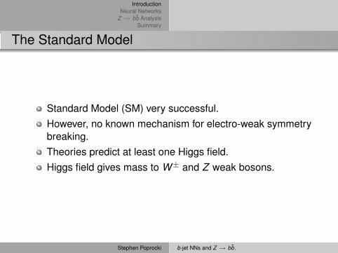
The Standard Model

Standard Model (SM) very successful.However, no known mechanism for electro-weak symmetrybreaking.Theories predict at least one Higgs field.Higgs field gives mass to W± and Z weak bosons.




Higgs Fields

Theories predict one or more Higgs bosons.Promising channels for Higgs detection at the Tevatron:

pp̄ →WH → lνbb̄,

pp̄ → ZH → l+l−bb̄,

pp̄ → ZH → νν̄bb̄.




Why b-jets

Calibration for b calorimeters.Measure mass of Z from Z → bb̄.Compare with known mass of Z .




Purity & Efficiency

Only use taggable MC jets.Each jet matched with 2 tracks within∆R =

√(∆η)2 + (∆φ)2 < 1.0.

Only use MC jets with at least 1 secondary vertex.Assume 0 vertex jets are non-b-jets.

efficiency =correctly tagged b-jetsnv>0

b-jetsnv>0 + b-jetsnv=0,

purity =incorrectly tagged non-b-jetsnv>0non-b-jetsnv>0 + non-b-jetsnv=0

.




TrainingMC Reconstruction OptionsImprovement Over Cut Method

Outline

1 Introduction



4 Summary





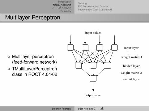
Multilayer Perceptron

Multilayer perceptron(feed-forward network)TMultiLayerPerceptronclass in ROOT 4.04/02

input values

output value

input layer

weight matrix 1

hidden layer

weight matrix 2

output layer





Training

Adjust weights according to output error.One weight update is an epoch/cycle/iteration.

Too many iterations =⇒ over-trained.Too few iterations =⇒ under-trained.

Various training algorithms.1 Stochastic minimization2 Steepest descent with fixed step size (batch learning)3 Steepest descent algorithm4 Conjugate gradients with the Polak-Ribiere updating

formula5 Conjugate gradients with the Fletcher-Reeves updating

formula6 Broyden, Fletcher, Goldfarb, Shanno (BFGS) method





Methods Training Error.

Epoch0 10 20 30 40 50 60

Epoch0 10 20 30 40 50 60

Err

or

0.2

0.25

0.3

0.35

0.4

0.45

0.5

Training sampleTest sample

iterations: 60method: Stochastic

Epoch0 10 20 30 40 50 60

Epoch0 10 20 30 40 50 60

Err

or0.2

0.25

0.3

0.35

0.4

0.45

0.5


iterations: 60method: Batch

Epoch0 10 20 30 40 50 60

Epoch0 10 20 30 40 50 60

Err

or

0.2

0.25

0.3

0.35

0.4

0.45

0.5


iterations: 60

method: Steepest Descent

Epoch0 10 20 30 40 50 60

Epoch0 10 20 30 40 50 60

Err

or

0.2

0.25

0.3

0.35

0.4

0.45

0.5


iterations: 60method: Ribiere Polak

Epoch0 10 20 30 40 50 60

Epoch0 10 20 30 40 50 60

Err

or

0.2

0.25

0.3

0.35

0.4

0.45

0.5


iterations: 60

method: Fletcher Reeves

Epoch0 10 20 30 40 50 60

Epoch0 10 20 30 40 50 60

Err

or0.2

0.25

0.3

0.35

0.4

0.45

0.5


iterations: 60method: BFGS





Methods Signal/Background & Purity V.S. Efficiency

NN output-0.4 -0.2 0 0.2 0.4 0.6 0.8 1 1.2 1.4

0

2000

4000

6000

8000

NN output-0.4 -0.2 0 0.2 0.4 0.6 0.8 1 1.2 1.4

0

2000

4000

6000

8000

b-jetsNon b-jets


NN output-0.4 -0.2 0 0.2 0.4 0.6 0.8 1 1.2 1.4

0

2000

4000

6000

8000

NN output-0.4 -0.2 0 0.2 0.4 0.6 0.8 1 1.2 1.4

0

2000

4000

6000

8000

b-jetsNon b-jets

iterations: 60method: Batch

NN output-0.4 -0.2 0 0.2 0.4 0.6 0.8 1 1.2 1.4

0

2000

4000

6000

8000

NN output-0.4 -0.2 0 0.2 0.4 0.6 0.8 1 1.2 1.4

0

2000

4000

6000

8000

b-jetsNon b-jets

iterations: 60

method: Steepest Descent

NN output-0.4 -0.2 0 0.2 0.4 0.6 0.8 1 1.2 1.4

0

2000

4000

6000

8000

NN output-0.4 -0.2 0 0.2 0.4 0.6 0.8 1 1.2 1.4

0

2000

4000

6000

8000

b-jetsNon b-jets

iterations: 60method: Ribiere Polak

NN output-0.4 -0.2 0 0.2 0.4 0.6 0.8 1 1.2 1.4

0

2000

4000

6000

8000

NN output-0.4 -0.2 0 0.2 0.4 0.6 0.8 1 1.2 1.4

0

2000

4000

6000

8000

b-jetsNon b-jets

iterations: 60

method: Fletcher Reeves

NN output-0.4 -0.2 0 0.2 0.4 0.6 0.8 1 1.2 1.4

0

2000

4000

6000

8000

NN output-0.4 -0.2 0 0.2 0.4 0.6 0.8 1 1.2 1.4

0

2000

4000

6000

8000

b-jetsNon b-jets

iterations: 60method: BFGS

Efficiency0 0.1 0.2 0.3 0.4 0.5 0.6 0.7

Efficiency0 0.1 0.2 0.3 0.4 0.5 0.6 0.7

Pur

ity

0.95

0.96

0.97

0.98

0.99

1

Stochastic

Batch

Steepest Descent

Ribiere Polak

Fletcher Reeves

BFGS





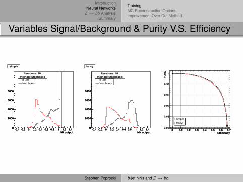
Variable Sets

Investigated mainly two variable sets:“simple”

1 3D decay length significance2 ∆R3 mass4 2D decay length5 χ2

6 multiplicity“fancy” = “simple” +

7 number of verticestertiary vertex:

8 3D decay length significance9 ∆R

10 mass11 χ2

12 multiplicity





Variables Signal/Background & Purity V.S. Efficiency

NN output-0.4 -0.2 0 0.2 0.4 0.6 0.8 1 1.2 1.40

2000

4000

6000

8000

NN output-0.4 -0.2 0 0.2 0.4 0.6 0.8 1 1.2 1.40

2000

4000

6000

8000

b-jetsNon b-jets


simple

NN output-0.4 -0.2 0 0.2 0.4 0.6 0.8 1 1.2 1.40

2000

4000

6000

8000

NN output-0.4 -0.2 0 0.2 0.4 0.6 0.8 1 1.2 1.40

2000

4000

6000

8000

b-jetsNon b-jets


fancy

Efficiency0 0.1 0.2 0.3 0.4 0.5 0.6 0.7

Efficiency0 0.1 0.2 0.3 0.4 0.5 0.6 0.7

Pur

ity

0.95

0.96

0.97

0.98

0.99

1

simplefancysimplefancy





Hidden Neurons

Compared performance of NNs with different number ofhidden neurons.6 hidden for “simple”.12 hidden for “fancy”.Two hidden layers did not help.





MC Reconstruction Options

MC data from 5 differentreconstruction optionswere compared.Default secondaryvertexing options wereworse than otherreconstruction options.

Efficiency0 0.1 0.2 0.3 0.4 0.5 0.6 0.7

Efficiency0 0.1 0.2 0.3 0.4 0.5 0.6 0.7

Pur

ity

0.95

0.96

0.97

0.98

0.99

1

cab3

cab_default_sv

cab_default-tj

cab_noadapt

cab_no-tj-merge

cab3

cab_default_sv

cab_default-tj

cab_noadapt

cab_no-tj-merge





MC Reconstruction Options

Improvement over previouscut on only 3D decay lengthsignificance.

Efficiency0 0.1 0.2 0.3 0.4 0.5 0.6 0.7

Efficiency0 0.1 0.2 0.3 0.4 0.5 0.6 0.7

Pur

ity

0.95

0.96

0.97

0.98

0.99

1

Neural Network

Cut Method




Background Subtraction

Outline

1 Introduction



4 Summary





NN Cut

≈ 100 pb−1 of DØ Run II data with Andy Haas’reconstruction options.Look for Z → bb̄ events using the NN.Cut on NN output to yield 50% efficiency and 99% purityfor b-tagging.






Background is essentially heavy-flavor dijet and mistaggedgluon/light-quark jet production.

Cannot be accurately simulated with current techniques.

Want to estimate background of double b-tagged data tosubtract it.Use a tag-rate function (TRF) to estimate the background.





Tag-rate function

M01_1tagsEntries 535909

Mean 202.7

RMS 106.1

(GeV)01m0 50 100 150 200 250 300 350 4000

0.02

0.04

0.06

0.08

0.1

0.12

0.14

0.16M01_1tagsEntries 535909

Mean 202.7

RMS 106.1

TRF derived from the single b-tagged data used to estimate thedouble-tagged background.





Background Comparison

(GeV)01m0 50 100 150 200 250 300 350 4000

500

1000

1500

2000

2500

3000

3500

4000M01_2tagsEntries 44257

Mean 89.67

RMS 37.86

Comparison between double b-tagged data (points) and theexpected background before any background corrections.






(GeV)01m0 50 100 150 200 250 300 350 400

-100

0

100

200

300

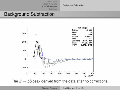
M01_2tagsEntries -491652Mean 120RMS 71.96

/ ndf 2χ 15.35 / 13Prob 0.2861Constant 43.0± 211.1 Mean 2.96± 61.63 Sigma 2.179± 9.978

The Z → bb̄ peak derived from the data after no corrections.





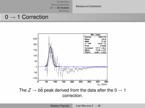
0→ 1 Correction

What is it?Double-tagged data has more heavy-flavor jets than thesingle-tagged data which the TRF is applied to.The difference in heavy-flavor jets is the 0→ 1 shift.

How to fix it?Compare untagged data with single tagged data.Subtract the 0→ 1 correction.





0→ 1 Correction

M01_1tagsEntries -2591179Mean 134.8RMS 77.45


(GeV)01m0 50 100 150 200 250 300 350 400

-100

-50

0

50

100

150

200

250

M01_1tagsEntries -2591179Mean 134.8RMS 77.45


The Z → bb̄ peak derived from the data after the 0→ 1correction.




Outline

1 Introduction



4 Summary




Summary

NNs yield better b-jet detection performance than a decaylength significance cut alone.Tertiary vertex NN variables don’t yield an improvement.MC reconstruction options can make a difference.Further corrections to the background subtraction areneeded.


Documents

Application of Neural Networks to b-quark jet detection … · Z → b¯b Analysis Summary Application of Neural Networks to b-quark jet detection in Z → bb¯. ... 2 Steepest descent