Embed Size (px)
Citation preview
SLAC-R-95-460 TOHOKU-HEP-OS-01
TOHOKU-HEP-NOTE-95-06 UC-414
A MEAkJiEMENT OF QUARK AND GLUON ’ JET DIFFERENCES AT THE Z” RFSONANCE
Yoshihito Iwasaki
Stanford Linear Accelerator Center Stanford University, Stanford, CA 94309
March 1995
Prepared for the Department of Energy under contract number DE-AC03-76SF00515
Printed in the United States of America. Available from the National Technical In- formation Service, U.S. Department of Commerce, 5285 Port Royal Road, Springfield, Virginia 22161.
l Ph.D thesis, Tohoku University
/ I
Abstract
We have studied the differences in properties between quark and gluon jets using 3-jet
events in hadronic decays of 2’ bosons collected by the SLD experiment at SLAC. Gluon
jets were identified in 3-jet events containing one jet tagged as a heavy quark jet. The tagged
gluon jets were compared with a mixed sample of light quark(u, d and s) and gluon jets, and
also with a mixed sample of heavy quark (c and b) and gluon jets. Our study shows that
the particle multiplicity of gluon jets is higher than that of light quark or heavy quark jets.
The ratios of average charged multiplicities of gluon and quark jets are measured to be
( ) n91uon _
(n!$~k) 1.29 f O.OG(stat.)~~:~~(syst.) ,
( ) ngfuon b$3
= 1.18 & O.OG(stat.)~~~(syst.)
These results are in quantitative agreement with QCD model expectations. Differences are
also observed in particle energy spectra and jet widths, consistent with naive QCD expecta-
tions. The experimental results are compared to Monte Carlo models of the hadronization
process.

Acknowledgements
I
First, I would like to thank the SLC/SLD collaboration for the successful construction I
and operation of the experiment.
I would like to thank Professor Haruo Yuta for his guidance as my thesis advisor.
And I would also like to thank Professor Koya Abe, who gave me the start of the
analysis.
In particular I would like to thank Phil Burrows for the many insightful discussions
and his encouragement. And thanks to the QCD group, Dave Muller, Mike Strauss, Hiro
Masuda, Takashi Maruyama, Mike Hildreth, Tom Junk, Jingchen Zhou and many others.
I would especially like to thank my fellows, Takaahi Akagi, Kazushi Neichi, Yoji
Hasegawa, and Yukiyoshi Ohnishi for the discussions about physics and life in general.
Many thanks to the whole SLD Tohoku group, Fumihiko Suekane, Tadashi Nagamine,
Shinya Narita, Haruhiko Araki, Kazumi Hasuko, Yoshinori Takahashi, Gou Shishido, and to
the Nagoya group, Ryoichi Kajikawa, Shiro Suzuki, Akira Sugiyama.
I thank my friends at Tohoku, Kyoko Tamae, Yumi Suzuki, Mssao Kuriki, Takayuki
Matsumoto, Syuichiro Hatakeyama, Hiroyuki Kawasaki, Masayuki Koga, Kou Fujita,
Atsushi Iwasaki, Mssahiro Onoda, Osamu Watanabe, Jun Yashima, Masatoshi Ishikawa,
Kouki Kawamorita, Takasumi Maruyama, Akihiro Kaga, Taksshi Kanno. Tetsuya Kineb-
uchi, Kouichi Kino, Kouji Maeda, Fuhito Nakanishi, Kaori Nanba, Mizuki Saitou, Toshikiyo
Tanaka, and Kenichi Takeuchi.
And finally, I thank my wife Yasuko and my family for their support and encourage-
ment.
ii
.
Contents
1 Introduction
2 Theoretical Backgrounds
2.1 Production and Decay of 2’ Gauge Bosons
2.2 Quantum Chromodynamics ..........
2.3 Quark and Gluon Jet Differences .......
2.4 QCD Models in e+e- Annihilation ......
2.4.1 The Matrix Element Method ......
2.4.2 The Parton Shower Method ......
2.4.3 Color Dipole Model ...........
2.5 Hadronization Models .............
2.5.1 String Fragmentation Model ......
2.5.2 Cluster Fragmentation Model .....
3 Experimental Apparatus
3.1 SLC . .
3.1.1 Beam Energy Measurement
3.2 SLD .
3.2.1 CCD Vertex Detector
3.2.2 Central Drift Chamber .
3.2.3 Endcap Drift Chambers
. . . 111
‘.
‘.
.
.
.
.
.
.
1
5
5
6
9
11
13
14
. 15
. 17
17
19
21
21
24
. 24
28
29
32
CONTENTS CONTENTS CONTENTS i CONTENTS
3.2.4 Cherenkov Ring Imaging Detector
3.2.5 Liquid Arkon Calorimeter
3.2.6 Warm Iron Calorimeter . .
3.2.7 Luminosity Monitor . . . .
3.2.8 Magnetic Coil . . .
3.3 SLD Monte Carlo . . . . . . .
3.4 SLD Event Reconstruction .
4 Event Selection
4.1 Data Taking
4.2 Event Topologies
4.3 Event Trigger
4.4 Offline Filter. . .
4.5 Hadronic Event Selection
4.6 Background Estimation
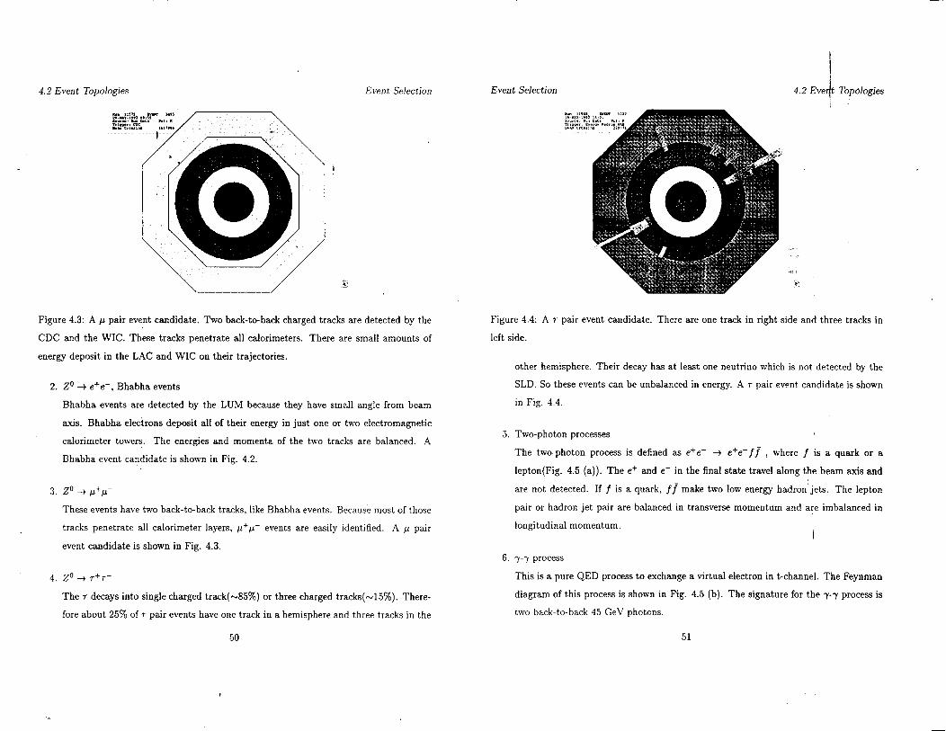
4.6.1 r+r- Events . . .
4.6.2 Two-Photon Processes
4.6.3 Beam Related Events
5 Analysis
5.1
5.2
5.3
5.4
5.5
Three Jet Event Selection
Flavour Tagging of Jets
Comparison of Jet Properties for Raw Samples
5.3.1 Charged Multiplicity .
5.3.2 Inclusive Energy Fraction
5.3.3 Jet Width . . . . . . . . . . .
Unfolding Distributions for Pure States
Comparison for Pure State Samples
5.5.1 Average Charged Multiplicity
iv
33
35 38
39
40
. . . 41
44
47
47
48
52
53
54
60
60
60
61
63
63
67
76
76
76
78
79
83
83
5.5.2 Average Inclusive Energy Fraction .................... 87
5.5.3 Average Jet Width ............................ 87
5.6 Systematic Errors ................................. 90
6 Summary 93
A SLD Collaboration 103
B Systematic Errors 109
C Monte Carlo Models 113
D Quark jet purity of the highest energy jet 121
LIST OF TABLES LIS t
OF TABLES
I
List of Tables
2.1 Z” properties. .......................
2.2 Summary of quarks. ....................
7
8
3.1 The SLC beam parameters. ................... 23
3.2 SLD subsystems. ......................... 27
3.3 The CCD vertex detector parameters. ............. 29
3.4 The CDC parameters. ...................... 31
3.5 The barrel CRID parameters. .................. 36
3.6 Main parameters of JETSET 6.3. ................ 41
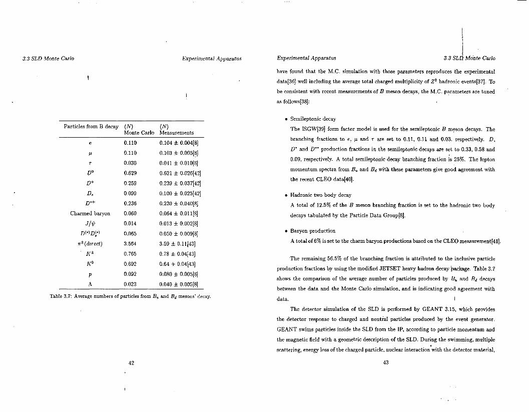
3.7 Average numbers of particles from l?, and Bd mesons’ decay. 42
4.1 Summary of track selection and hadronic event selection.
4.2 Summary of 7i+r- event multiplicity. . . . .
59
61
5.1
5.2
5.3
5.4
5.5
5.6
5.7
Summary of 3-jet event selection. .............
Summary of three jet samples. ..............
Jet properties of three samples. ..............
Summary of the composition and the correction matrices.
Fitted values and reduced x”. ...............
The final ratios of gluon to quark jets. ..........
Summary of systematic errors. ...............
68
72
80
84
84
86
91
B.l Systematic errors. . . . . . . . . . . . . . 112
vi
C.l Main parameters of the HERWIG 5.7. ............... .’ ...... 113
C.2 Main parameters of the ARIADNE 4.06. .................... 114
C.3 x*/Nd, of M.C. model comparison. ....................... 116
D.l Fraction of heavy tagged jets. .................. : ........ 123
D.2 Fraction of quark jets. .............................. 123
vii
List of Figure’s
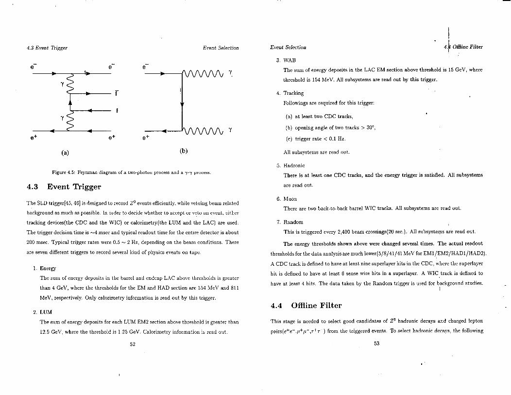
2.1 The fundamental processes of e+e- + ff. .
2.2 Schematic illustration of e+e- + hadrons. .
2.3 Schematic illustration of a parton shower. .
2.4 Schematic illustration of the color dipole mode!.
2.5 Schematic illustration of the string fragmentation mode!.
2.6 Gluon radiation in the string mode!. . . .
2.7 Schematic illustration of cluster mode!. .
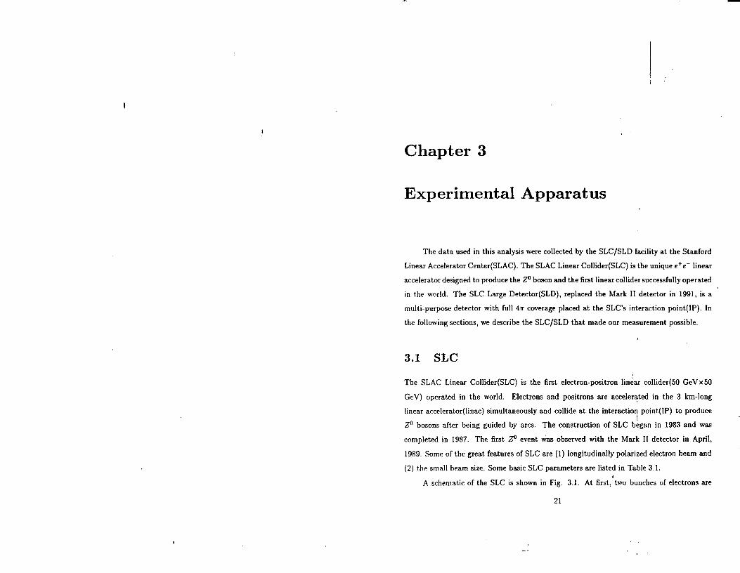
3.1
3.2
3.3
3.4
3.5
3.6
3.7
3.8
3.9
Schematic view of the SLC. . . . .
Schematic of the SLC beam-energy spectrometer.
A quadrant schematic view of the SLD.
SLD coordinate system.
The CCD vertex detector. . . .
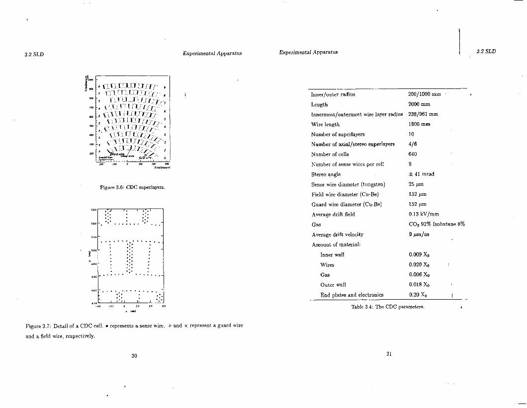
CDC superlayers. .
Detail of a CDC cell. .
Cherenkov angle.
Schematic view of the barrel CRID. . .
. 6
12
14
16
17
18
19
3.10 Schematic of the CRID drift box. ......................... 35
3.11 Schematic of LAC segment. ........................... 36
3.12 Schematic of LAC. ....................... : ........ 37
3.13 Schematic of the WIC layers. .......................... 38
LIST OF FIGURES LIST b F FIGURES I ,’
3.14 Schematic of the LUM. .......................
3.15 CDC vector hits with fitted tracks. .................
3.16 CDC hits linked to the CDC tracks. .................
4.1 A hadronic event candidate with 4-jet event shape.
4.2 A wide angle Bhabha event candidate.
4.3 A p pair event candidate. . . . .
4.4 A r pair event candidate. . . . . . .
4.5 Feynman diagram of a two-photon process and a y-y process. .
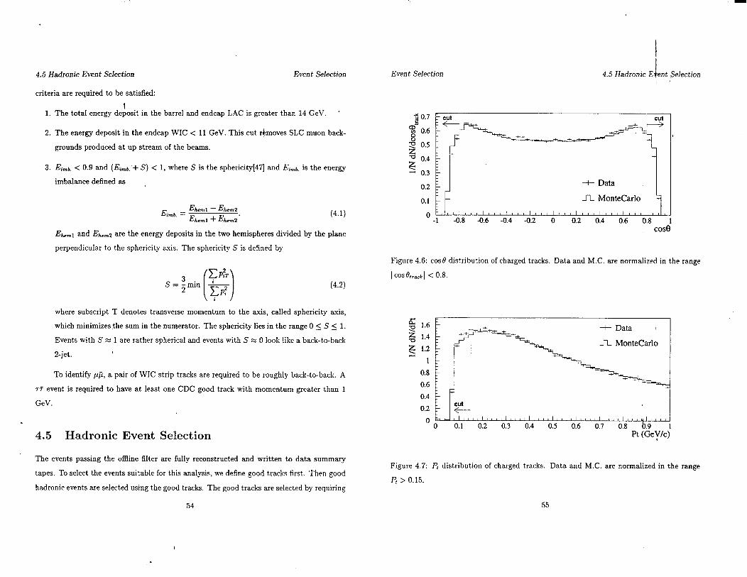
4.6 cos0 distribution of charged tracks. .
4.7 Pt distribution of charged tracks. .
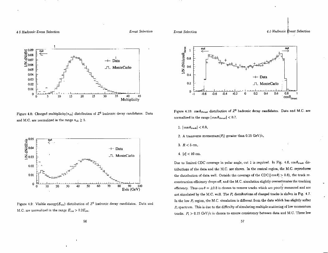
4.8 Charged multiplicity distribution of Z” hadronic decay candidates.
4.9 Visible energy distribution of Z” hadronic decay candidates.
4.10 COS&hrust distribution of Z” hadronic decay candidates. . .
5.1 n-jet rates a5 a function of yeut. ....................
5.2 Definition of variables for 3-jet event. .................
5.3 cosQj,t distribution of jets in 3-jet events. ...............
5.4 Euis distribution of jets in 3-jet events. .............. ..
5.5 C 4, distribution of jets in 3-jet events. ................
5.6 A hadronic event candidate with three jets. ..............
5.7 Definition of the impact parameter. .............. ‘. ..
5.8 Weighted impact parameter(o’“P ) distribution. ............
5.9 Three samples of tagged jets. ............. : .......
5.10 A 3-jet event with a gluon tagged jet. .............. ,’ ..
5.11 Ej,t distribution of three samples. ..................
5.12 Average charged multiplicities. ....................
5.13 Inclusive energy fraction(XE). .....................
5.14 Average jet width. ...........................
. 39
44
. 45
48
49
50
51
. . 52
. 55
55
56
56
57
. 64
64
65
65
65
68
. . . 69
69
73
74
. 75
77
. 78
. 79
viii
LIST OF FIGURES LIST OF FIGURES
5.15 Average charged multiplicities (n,,,) and their ratios. ............. 85
5.16 Average inclusive edergy fractions (XE) and their ratios. ........... 88,
5.17 Average jet widths (0) and their ratios. .................... 89
6.1 Summary of recent measurements of the multiplicity ratio. . . 95
C.l M.C. comparison of (nh) ............................ 117
C.2 M.C. comparison of (X,) ............................ 118
C.3 M.C. comparison of (0) .............................. 119
D.l Energy spectra of jets in 3-jet events . . . . 124
X
I
Chapter 1
Introduction
Quantum Chromodynamics, QCD, is a non-Abelian local gauge invariant field theory
which describes the strong interactions between colored quarks and gluons. It is a fundamen-
tal element in the standard model of the known interactions(except gravity) of elementary
particles. QCD was developed as an analogy of QED(Quantum Electrodynamics). QED
provides accurate theoretical predictions which have been tested by experiments with high
precision. On the contrary, QCD tests are rather less precise due to the complexity of phys-
ical properties involved in &CD: asymptotic freedom and color confinement. Asymptotic
freedom means that the effective strong coupling constant decreases logarithmically at short
distances so that we can apply perturbation theory to QCD in large momentum transfers.
However, the strong coupling constant is still large enough so that the higher order correc-
tions, which could give significant shifts to current theoretical predictions’are not calculable
with high precision even in the large momentum transfer regime. Color cbnfinement means
that the potential energy between color charges increases approximately linearly at large dis-
tances, so that quarks are confined in hadrons. Therefore, we can not observe bare quarks
and gluons, the elementary fields of QCD, but can observe colorless bound states of these
constituents, hadrons.
From these reasons, it is very hard to derive properties of the quark-gluon interactions
Introduction Introduction
from the hadronic states. QCD analysis of high energy experiments are done in the frame-
work of the QCD-improveh parton models. In other words, we have to use some models with
perturbative QCD approximation, QCD-improved parton models, to extract basic features I of QCD from the hadronic final states which we observe. As a consequence of such difficulties
in QCD measurements, not only single experiment but many experiments are required to
test qualitative QCD predictions and QCD models.
A comparison of quark and gluon jet properties is one of the long-standing difficult
problems in &CD. This is due to the difficulty of gluon jet identification on the experimental
side and the difficulty of subasymptotic corrections on the theoretical side. Lowest order
QCD predicts 9/4 for the multiplicity ratio of gluon to quark jets. This value is expected
from the color charge ratio of gluon(C’A = 3) to quark(CF = 4/3). For quark and gluon jets
with equal energy, this multiplicity ratio implies that gluon jets have a softer particle energy
spectrum compared with quark jets. We can also expect that the angular distribution of
particles relative to the jet axis in gluon jets is wider than that in quark jets because the
mean transverse energy of the particles is about the same. However, these naive expectations
are substantially reduced due to higher order corrections. The multiplicity ratio of hadrons
in quark and gluon jets, for instance, is corrected to 1.38 f 0.02 in a recent QCD calculation
with a hadronization model[l].
a measurement using Z” hadronic decay data collected by the SLC Large Detector(SLD)
experiment at SLAC’. About 250 members from 34 institutions collaborate on the SLD
experiment*. The SLAC Linear Collider(SLC) is the first e+e- linear collider successfully
operated at the Z” peak, and produces 2’ events with the small and’stable Z” production
point. The SLD with its precise vertex detector has excellent efficiency for separating heavy
hadrons’ secondary vertices from the primary vertex. These SLC/SLD features and our
analysis method allow efficient flavour tagging of jets in Z” hadronic events with high purity,
and make the gluon jet analysis possible even with smaller data sample than the LEP
experiments. The efficient flavour tagging of jets in this experiment is one of the motivations
for this study. The first engineering run was carried out in 1991, the physics run started in
1992 and data are still being taken. This thesis is based on about 63,000 Z” hadronic decay
data taken in 1992 and 1993 runs.
The content of this thesis is organized as follows. In chapter 2, some foundations of
QCD relevant to this study are reviewed. Experimental apparatus is described in chapter
3. In chapter 4 the details of the event and track selection procedures are presented. The
analysis method and the results are presented in chapter 5. Finally, the conclusion is given
in chapter 6. In appendices, Monte Carlo models of hadronization process are compared to
the experimental results, and the systemtic errors are discussed.
Experimental searches for the differences between quark and gluon jets have been
performed in the experiments of e+e- and pp collisions, and some indications of quark and
gluon jet differences were reported[2, 31. However, some of their analyses based on the
comparison of quark jets from one experiment and gluon jets from other experiment, and
relied on Monte Carlo simulations. Thus, their results were indirect, and would be biased hy
the different experimental environments and by the choice of the Monte Carlo simulations.
Recently, analyses with high statistics data were performed by the LEP experiment[4, 5, 61.
They performed the direct comparison using symmetric 3-jet events in Z” hadronic decays
and reported significant differences. ‘Stanford Linear Accelerator Center
In order to search for the differences between quark and gluon jets. we have performed *The institutions and the members of the SLD collaboration are listed in Appendix A
2
Introduction 1 Introduction I
Introduction Introduction
I
.
i
Chapter 2
Theoretical Backgrounds
In this chapter, we review the decay of 2’ gauge bosons produced by e+e- annihila-
tion which provides us an excellent experimental environment to study &CD. Then, some
foundations of QCD relevant to this study are outlined, and the differences between quark
and gluon jets are discussed with the experimental measurements. As described in chapter
1, experimental QCD studies have to employ some phenomenological QCD models for the
parton evolution and the hadronization process. Thus, we give a brief explanation of the
models used in this analysis.
2.1 Production and Decay of 2’ Gauge Bosom
The fundamental process of electron-positron annihilation is e+e- -+ !J, where
f = e, ,LL, r, v,, v,,, vrr u, d, s, c, b at the 2’ mass energy. There are twolbasic neutral gauge
bosons which contribute to this process: the photon and the 2’. The Feynman diagrams of
the lowest order electron-position annihilation(except for e+e- + e+e-) are shown in Fig.
2.1. The cross section, U, of efe- + ff at the center of mass energy, 4, close to the
mass of Z”, Mz, is proportional to square of the sum of matrix elements of two diagrams,
JM, + Ms12: a pure electro-magnetic interaction term, a pure weak interaction term and
an interference term of the two interactions. At 6 = Ms, the interference term vanishes.
4 5

Theoretical Backgrounds 1 2.2 Quantum Chi omodynamics 2.2 Quantum Chromodynamics Theoretical Backgrounds
-. lZO _,---_
(a) * (b) Figure 2.1: The fundamental processes of e+e- + jf
Therefore, the weak interaction dominates because the electro-magnetic interaction is small
at the Z” pole. (uwra~/uem - 1100). In this case, the lowest order differential cross section
at the Z” mass energy is written in a simple form[7] by neglecting the initial and final state
fermion masses as
(2.1)
where A4z and Tz are the mass and totaI decay width of Z”, 6’ is the angle between the
initial electron and final fermion, o is the fine structure constant. v,, a,, VI and al are the
vector and axial vector couplings to Z” gauge boson for electron and fermion, respectively.
The Z” mass, width and branching ratio to each fermion pair are listed in Table 2.1[8].
2.2 Quantum Chromodynamics
Since the discovery of the n meson in 1947, a large collection of hadron mass spectra and
hadronic interactions in high energy experiments strongly suggested that there exist point-
like structures within hadrons. In 1968, the deep inelastic electron-proton scattering exper-
iment at SLAC observed the first direct evidence for quarks, which carry roughly one third
of the nucleon energy. In 1972, QCD[9, 10, 11) was born in the form of a simple and elegant
Z” maas
Z” decay full width(I’,)
91.187 f 0.007 GeV/c2
2.490 3~ 0.007 GeV
Z” decay branching fractions
e+e- ( 3.366 f 0.008 )%
P+P- ( 3.367 f 0.013 )%
r+r- ( 3.360 f 0.015 )%
invisible ( 20.01 f 0.16 )%
hadrons ( 69.90 f 0.15 )%
(UE + E)/2 ( 9.7 4~ 1.8 )%
(dd+ s8+ b6)/3 ( 16.8 * 1.2 )%
’ CC ( 11.9 f 1.4 )%
b6 ( 15.45 * 0.21 )%
Table 2.1: 2’ properties. I
6
.
7
2.2 Quantum Chromodynamics Theoretical Backgrounds Theoretical Backgrounds
Flavour I , 13 S C B T Q/e mass
d 112 -l/2 0 0 0 0 -l/3 5 to 15 MeV/c2 ’
U 112 l/2 0 0 0 0 +2/3 2 to 8 MeV/c?
S 0 0 -1 0 0 0 -l/3 100 to 300 !vleV/c2
C 0 001 0 0 +2/3 1.0 to 1.6 GeV/c2
b 0 0 0 0 -1 0 -l/3 4.1 to 4.5 GeV/c?
t 0 0’ 0 0 0 1 +2/3 174 f lO?$ GeV/r?
Table 2.2: Quark summary. Top quark mass is from a CDF observation of top candidate
events. B indicates quantum numbers of bottomness, not baryon numbers.
Lagrangian based on the gauge group SU(3),,,0r. In 1974, a new particle, the J/g, was
discovered at SLAC and Brookhaven simultaneously, and was interpreted as a bound state
of d. Subsequently, the Y was discovered at FNAL in 1977, which is a bound state of b6, a
bottom quark and an anti-bottom quark. After the discovery of charm and bottom quarks,
our quark table(Table 2.2) has enlarged.
Five quark flavours out of six flavours have been found experimentally. The top quark
(sixth quark) has been suggested to exist at 150-180 GeV by the radiative corrections of
higher order weak inter’actions[8]. Recently. the CDF collaboration has observed a possible
signal of the top quark[l2]. Q uar k s are spin l/2 fermions with fractional charges of +ie for
up type quark(u, c, t) and -3e for down type quarks(d, s, b). Quarks can carry one of three
strong charges, called color charges, say Red, Blue or Green conventionally. Anti-quarks
can carry the corresponding anti-color. The color symmetry is supposed to be exact, thus
the strong interaction is independent of colors. The boson intermediating strong interaction
between quarks is named the gluon. The gluon is a spin 1 massless boson and carrys a color
and an anti-color or their combinations(RB, Rc;, Bc?‘, Bl?, Gi?, Gl?, -&(Rl?- BL?), -&(RR+
BB - 2Gc)). The color charge in strong interactions is analogous to the electric charge in
electromagnetic interactions. In both interactions, a massless spin 1 boson(a photon or a
8
2.3 Quark and Gluon t
et Differences
gluon) mediates the force. The important difference between them is that phbtods have no
charge, while gluons have. Therefore, gluons can interact with other gluons, whereas photons
can not interact with each other. The existence of this direct coupling of gluons differentiates
the charge screening of QCD from that of QED. The resulting “anti-sc!eening” of the color
is referred to as “asymptotic freedom”. This means that the strength of the interaction
between quarks decreases as the distance between them decreases, and the state of quarks
approaches to be free asymptotically. This behavior allows us to use perturbative QCD
calculation for short distances. On the contrary, at long distances, quarks interact strongly
and so can never escape. This is, called “confinement of quarks(and gluons)“: corresponding
to the hadronic states. Perturbation theory is not applicable for the hadronization process of
quark and gluons because the coupling is so strong. Thus, we have to use phenomenological
models to describe such states.
2.3 Quark and Gluon Jet Differences
In QCD, gluons are massless, spin 1 bosons with color charge which should be 9/4 times as
large as that of quarks. In this section, we briefly review the quark and gluon jet differences
in terms of particle multiplicities in jets.
The color charge of the quark, C F, is 4/3 and that of the gluon, Cc, is 3. This means
that the three-gluon coupling, which determines the properties of gluon jets, is stronger
than the 999 coupling relevant to quark jets. Therefore, we can naively expect that the
multiplicity in gluon jets is higher than that in quark jets. Correspon’dingly, the energy
spectrum of particles in gluon jets is expected to be softer than that ih quark jets. The
distribution of the angle between the particle and the jet axis in gluon jets is also expected
to be wider than that in quark jets because the mean transverse energy of gluon radiation
in both jets is expected to be about the same.
The multiplicity ratio, R, of gluon jets to quark jets is given as the ratio of color charges
9
2.3 Quark and Gluon Jet Differences Theoretical Backgrounds
in the lowest order QCD prediction,
I R = CG/CF = 914. (2.2)
This lowest order R value is not too small to be observed experimenthlly. When higher order
corrections are taken into account[l3], however, this ratio is reduced to
R = $1 - 0.276 - O.O7a,]. (2.3)
Recently, R was calculated by using the exact solution of QCD equations for generating func-
tions with fixed coupling[l]. Th e ratio of parton(see Chapter 2.4) multiplicities is predicted
to be
R parton = 1.84 f 0.02. (2.4)
By the use of the HERWIG Monte Carlo simulation[l4], Rpartcn is related to the hadronic
ratio Rhadron which can be measured by experiments
R RM C
hadron = Rparton$$= partO”
= 1.38 f 0.02, (2.5)
where REFtO, and RF$&, are the ratios for partons and hsdrons in the Monte Carlo, respec-
tively. Thus, R is significantly reduced by the hadronization process in the prediction.
Experimentally the HRS collaboration has measured the ratio of charged multiplicities
&h with symmetric 3-jet events in e+e- annihilation at PEP[3]. In the analysis, the sym-
metric 3-jet events were collected in which all jets were produced with a relative angle of 120
degrees in the event plane and had the same jet energies Ej.t = G/3. Thus, the probability
of a jet originating from a gluon is the same for each jet in the event. From Monte Carlo
simulations, they estimated that the charged multiplicity of quark jets at fi = 2Ej,, is
5.2. To obtain the charged multiplicity of gluon jets, a model with Poissonian multiplicity
distribution is assumed. The model reproduces the measurement with the charged multi-
plicity of gluon jets equal to 6.7:::; f 1.0. Therefore, the charged multiplicity ratio &, is
1.29$:~+0.20, indicating no significant difference in the charged multiplicity between quark
and gluon jets within the quoted error.
10
Theoretical Backgrounds
The OPAL, DELPHI, and SLD collaborations have measured the ratios of multiplic-
ities, energy spectra and jet widths using different type of symmetric 3-jet events in Z”
hadronic decays[5, 6, 151. They select the symmetric 3-jet events, in which the angles from
the highest energy jet to other two jets are the same. In such an event configuration,, the
highest energy jet is a quark jet with high probability. Thus the two lower energy jets are
a quark and a gluon jets. If one of the two jets is tagged as a heavy quark jet, then the
remaining jet is anti-tagged as a gluon jet. The multiplicity ratios measured by OPAL are
R = 1.267 f 0.043 f 0.055 : Ej,r = 24GeV,
&h = 1.326 f 0.054 f 0.073 : Ejct = 24GeV. (2.6)
where R,,, is the ratio of the charged multiplicities. The DELPHI collaboration has measured
R = 1.22 f 0.04 : Ejc, = 30GeV,
R = 1.172f 0.032 : 15 < Ejet < 39GeV. (2.7)
All the values are significantly larger than unity, indicating that the multiplicity of gluon
jets is larger than that of quark jets. However, the ratios R are somewhat smaller than the
prediction given by eq. 2.5. The preliminary result measured by the SLD collaboration is
gluon/lightquark 8, = 1.36 f 0.24 : Ej.at = 24GeV. (2.8)
This is the charged multiplicity ratio of gluon to light quark jets. Thus, we can not compare
this value with the OPAL and the DELPHI results directly.
2.4 QCD Models in e+e- Annihilation I
The evolution of hadron jet in e+e- annihilation takes place in four phases by means of
the interactions and models, as shown in Fig. 2.2. In the first phase, the initial e+e- pair
annihilates into a gauge boson, a photon or a Z”, which in turn decays into a quasi free pair
of quark and anti-quark. This process is well described by electro-weak theory, as explained
11
2.4 &CD Models in e+e- Annihilation Theoretical Backgrounds
e+
e’
Figure 2.2: Schematic illustration of e+e- --f hadrons.
in section 2.1. In the second phase, QCD plays an important role, and thus the differences
between quark and gluon jets are caused. Gluons are radiated from initial quarks, and in
turn gluons may radiate gluons, or create quark antiquark pairs. The quarks and gluons
in this phase are called “partons”. In principle, there are two approaches for calculating
parton configurations[l6, 171: Matrix Element(ME) and Parton Shower(PS) methods. The
ME is the exact QCD.matrix elements that has been calculated up to second order(U(crz),
up to 4-parton production). The PS is the leading logarithmic approximation of QCD,
and is formulated as a branching process of virtual partons according to the Altarelli-Parisi
equations[l8]. In the third phase, hadrons are generated from partons. This phase can not yet
be calculated in &CD, as described in chapter 1. Thus, phenomenological parameterization
of hadron production must be used to describe this phase in Monte Carlo simulations. In
the last phase, hadrons decay into stable hadrons and leptons, which can be observed by
experiments. In the following sections, we review the QCD models used in the second and
third phase.
12
Theoretical Backgrounds 2.4 &CD Models in e e- Annihilation j :
2.4.1 The Matrix Element Method
The standard approach of calculating the hadronic cross section is the Matrix Element
method in which we calculate the amplitude of Feynman diagrams up to a fixed order of
0,. To get the rate of N-parton production, the matrix elements de added and squared, *
then integrated over the phase space. According to the N-parton fraction determined by the
matrix elements, the multiplicity of partons and 4-momentum of partons are determined in
a Monte Carlo simulation.
The first order QCD correction to e+e- + qtj is the gluon radiation from the q or Q.
The differential cross section for this configuration(e+e- --t qqg, 3-parton) is calculated[l9]
for massless quarks as
da as 2 x: + x; -=00Yz(1-21)(1-z2)’ dx,dxz (2.9)
where oo is the cross section for e+e- + qq, x,,z~ and 53 are the scaled energy variables in
the CM frame of the event
XI = 2-f-7, 1x6
12 =2Ei /A,
x3 =2Eg /&. (2.10)
The kinematically allowed region is 0 5 xi 2 l(i=1,2,3). For x1 or 22 !+ 1, the cross section
for 3-parton(eq. 2.9) diverges. However, the divergence is canceled when the first order
propagator and vertex corrections are taken into account. This cancellation corresponds to
a difficulty to distinguish a gluon from a quark which is soft or collinkar to the quark. In
a Monte Carlo, the divergence is solved by a cut-off maas of two partons(a quark and a
gluon):a gluon is radiated if the virtual mass of the gluon and quark is larger than a certain
cut-off mass. In other words, events with a hard gluon are generated according to the cross
section in eq. 2.9, but events with a soft or collinear gluon are combined to 2-parton events.
13
2.4 QCD Models in e+e- Annihilation Theoretical Backgrounds Theoretical Backgrounds
Figure 2.3: Schematic illustration of a parton shower. Lines and spirals represent quarks(or
anti-quarks) and gluons, respectively.
In second order &CD, two new parton configurations are added to the first order
configurations:e+e- + qqgg and e+e- + q&‘$. The cross section of 4-parton events has
been calculated by several groups[20]. The same rules as 3-parton calculations can be applied
to 4-parton configuration. As in the 3-parton case, divergences appear, but are removed by
the cut-off mass.
2.4.2 The Parton Shower Method
The Parton Shower method is based on the leading-log approximation of perturbative
&CD. The initial quarks are produced with off-shell mass, and decay(or branch) into virtual
partons which in turn decay(Fig. 2.3). Progressive branchings continue until they reach a
certain cut-off mass Qs. In this method, only the leading logarithmic terms in the pertur-
bative QCD expansion of the two body decay cross section are used. The basic branchings
are
14
2.4 QCD Models in e+
(2.11)
where q(q) and g represent a quark(anti-quark) and a gluon, respectively. The Altarelli-Parisi
splitting kernels for the parton branchings[l8] are
P g-Q+9 = 2C& - 2 + 2)
t(1 -z) ’ P g-‘s+P = TR(2 + (1 - 2)s) (2.12)
where Cp and Co are the color charges of quark(4/3) and gluon(3) respectively, and Ta =
N,/2, where N, is the available number of quark flavours for quark pair creation. The
probability distribution for this branching is given by
dP,+btc -= dt /
dt-P.+b+&) 297
(2.13)
where t is the evolution parameter(t = ln(Q2/A2)) and z specifies the fraction of four-
momentum for daughter b. In this model, no interference between branchings is taken into
account. The PS Monte Carlo has only two parameters:the leading-log QCD scale A and
the cut-off mass Qs. An advantage of the PS compared to the ME is that we can generate
more than 4 partons, which is the current limit of number of partons generated by the ME.
The maximum number of partons in the PS is determined by the cut-off ‘mass Qu.
2.4.3 Color Dipole Model
In the case of e+e- annihilation, perturbative QCD can be formulated in an alternative in
terms of quarks and gluons or in terms of color dipoles. The Color Dipole Model(CDM)[24,
15
2.4 &CD Models in e+e- Annihilation Theoretical Backgrounds
Figure 2.4: Schematic illustration of the color dipole model.
251 is baaed on the fact that an emission of a gluon from a qQ pair can be treated as a radiation
from the color dipole between quark and anti-quark(Fig. 2.4(a) and (b)). The emission of a
second gluon is treated as radiation from two independent dipoles: one stretched from the
quark to the gluon and the other from the gluon to the anti-quark(Fig. 2.4(b)). This process
is generalized so that one more gluon is given by three independent dipoles, etc(Fig. 2.4(c)).
There are three different types of dipole:the dipoles between a quark and an antiquark,
between a quark and a gluon, and between two gluons. The cross section for gluon emission
from the dipoles are calculated[23] as
du 2% w ‘W9 :yg&=u-
x: + xi 37r (1 - x1)(1 - 5s)’
do 3% !a --f Q99 : d;cldzg = u-
x: + x; 47T (1 -x1)(1 -x3)’
du 3% 99 -+wg :==u-
xi + x; 47r (1 -x1)(1 - 1s)’
where xi are the final state energy fractions, 2E,/+, of the emitting partons in the center
of mass system of the dipoles
16
Theoretical Backgrounds 2.5 Hadro rl ization Models
-0 -@ o-0 - q M9’ q’- 9
Figure 2.5: Schematic illustration of the string fragmentation model.
2.5 Hadronization Models
In this section, two conventional hadronization models relevant to this study will be re-
viewed:the String Fragmentation(SF) and Cluster Fragmentation(CF) models. In the SF,
the color confinement is a basic concept: hadrons are produced from colorlessstring systems,
not from isolated colored quarks. In the CF, hadronization process is described by massive
colorless objects like the SF. But important difference between the CF and the SF is that
no assumptions of fragmentation functions of partons are needed in the CF as a result of
colorless clusters.
2.5.1 String Fragmentation Model I
The String Fragmentation(SF) model is implemented in the JETSET Monte Carlo program[21].
The string model for qrj system is basically a simple color confinement picture for hadroniza-
tion. The main assumption of the SF model is that the fragmentation of outgoing partons
are not independent. In the SF, a virtual string is considered to be a color flux tube be-
17
h 2.5 Hadron : ation Models i
HALIRONS
HADRONS
HADRONS
HADRONS
2.5 Hadronization Models Theoretical Backgrounds Theoretical Backgrounds
e+
e-
(a) (b)
Figure 2.6: Gluon radiation in the string model:(a)a kink of a string. (b)virtual strings in Figure 2.7: Schematic illustration of cluster model. Dotted lines represent color flows.
The longitudinal fragmentation is formulated in terms of a probability distribution
f(z). z is the fraction of the energy given by the initial qq pair to the newly created hadron.
In JETSET,
4 f(z) - i(l- z)‘exp(+) (2.16)
is used with the parameter value a = 1 and b = 0.7.
In the SF model, gluons correspond to kinks on the string spanned between a quark
and an antiquark. Thus, a gluon has two string pieces attached to it, while a quark or an
antiquark has one string(Fig. 2.6).
2.5.2 Cluster Fragmentation Model I
The first Cluster Fragmentation(CF) model was presented by Field and Wolfram[22]. In
the CF model, hard color separations are neutralized before hadrons are actually formed.
This color screening process is interpreted as the initial state is evolved into a collection
of low mass colorless clusters. So the role of the QCD dynamics is limited to describing
19
the CMS.
tween partons(Fig. 2.5). The transverse dimension of the tube is roughly 1 fm. As the
partons move apart, the string is stretched. Thus, the potential energy stored in the string
is increased and the string may break by a new q’d pair creation. In this manner the initial
state qq system splits into two color singlet systems, qg and q’q. This string stretching and
breaking process may occur until invariant masses of qQ are small enough. After this process,
hadrons are formed by the quark from one break and the anti-quark from adjacent break.
When the q’q pair is created by the breaking of the string, transverse momenta are
give to q’ and 3. The production probability is proportional to
exp(-zm$/fc) = exp(-rm2/K) exp(-?rPG/K), (2.15)
where mr is called transverse mass, mp is the virtual mass of the newly created quark, and
PT is the transverse momentum. The default value of PT in JETSET is 0.40 GeV. Eq. 2.15
also gives relative rates for the production of quark flavour on the basis of quark mass(u:d:s:c
M 1:1:0.3:10-1’).
18
.-
2.5 Hadronization Models Theoretical Backgrounds
the production of this final cluster states. In this model, no assumptions of fragmentation
functions of partons are u&d. This is the important difference between the CF and the SF
model described in previous section.
After the parton shower is generated from initial quarks, final-itate partons are put on
maas shell. Then final-state gluons are split into qq pairs
9[Pl -+ +Pl+ a1 - 4Pl> (2.17)
where g and q represent a gluon and a quark with 4-momentum p and rp. Several choice
were tried for the probability function of .a. In this process, color flows between partons are
formed(dotted lines in Fig. 2.7), and the color charge is assigned to quark(Fig. 2.7). Then
final state quarks are linked to a unique parton partner, anti-quark, by the color charge
information, and form clusters. The clusters have a mass M and quark flavours of q and 8.
These clusters are then simply decayed into two hadrons
Ci(M~%~Gb) + HI + HZ, (2.18)
where C, and H represent a cluster and a hadron. The probability of the decay is given by
P(C,+H,+H2)=PF.Ps.PK (2.19)
where Ps is the number of spin state of final hadrons, PK is a 2-body phase space suppression
factor and PF is an available flavour factor of final hadrons. The decay mode is chosen from
all possible decays at random with the individual flavor factor weight. Unstable hadrons
produced in clusters are decayed subsequently until stable hadrons are produced.
20
i
3.1 SLC Experimental Apparatus Experimental Apparatus
Polohmeter ,
Polorired e- Soul xe POLARIZATION IN THE OVERALL SK iAYOUT
10.86 5511*4
Figure 3.1: Schematic view of the SLC.
22
Year 1992 1993
EC773 91.55 GeV 91.26 GeV
Electron polarization 22.4% 63.0%.
Number of electrons/bunch 3.0 x 10’0 3.5 x 10’0
Number of positrons/bunch 3.0 x 1O’O 3.5 x 10’0
Beam size 2pm x 2pm 2.3pm x 0.8pm
Bunch length 1.2mm 0.6mm
Table 3.1: The SLC beam parameters.
created by photoemission from a GaAs photocathode at the polaiized electron source. Those
bunches are accelerated to 0.2 GeV by the energy booster and to 1.0 GeV by a linac and
are transported to the North Damping Ring. In the South Damping Ring, two bunches of
positrons are accumulated(we describe positron creation later). ‘In the damping rings, the
emittance of each bunch is reduced. One bunch of positrons is extracted from the South
Damping Ring and then injected into the linac. The pulse compressor reduces the bunch
length from 1 cm to 1 mm. After the positron bunch, two bunch of electrons are also injected
into the linac. The distance of those bunches are 17.6 m. First two bunches(positrons and
electrons) are accelerated to 46.7 GeV before entering the South and North Arc, respectively.
The last bunch of electrons is accelerated to 33 GeV, extracted from the,linac and guided to
a Tantalum-Tungsten target to produce positrons. In the target, posit&is are produced by
pair-creation from the bremsstrahlung of electrons, and are collected by a focusing solenoid.
Positrons are transported back to the beginning of the linac by the Return Line, and then I
accelerated to 1.0 GeV to transported to the South Damping Ring. In the meantime, the
first two bunches of positrons and electrons accelerated up to 46.7 GeV are split by a dipole
magnet at the end of the linac and transported through the SLC arcs toward the interaction
point. The bunches are focused in Final Focus System(FFS) to brder of 1 pm of transverse
size at the interaction point. The beams are crossed at the IP, and then the beams are kicked
23
3.2 SLD Experimental Apparatus
into the extra&ion lines and led to the north and south beam damps.
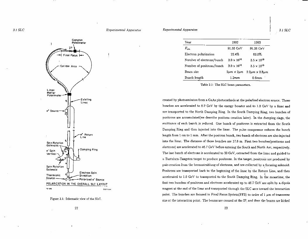
3.1.1 Beam Energy Measurement
The beam energy spectrometers are located at the end of the beam transport system, 150
m past the IP, on the south arc for electrons and on the north arc for positrons. The beam
energies of positrons and electrons are measured by bending the beams through three dipole
magnets shown in Fig. 3.2. The deflection angle 0 is related to the beam energy by the
expression,
E beam = - ;p x Bl (3.1)
where J3 is the magnetic filed of the analyzing magnets and dl is the path length in the
analyzing magnet along the beam. The deflection angle is measured by the Wire Imaging
Synchrotron Radiation Detector(WISRD)[26]. The first and third small magnets in Fig.
3.2 sweep the beam horizontally, creating parallel stripes of synchrotron radiation. The
second magnet bends the beam down by 18.286 mrad. The distance between two stripes is
measured by the WISRD 15 m away. The WISRD has two screens of copper wires which
detect compton scattering of the electrons in the screens. During the 1992 and 1993 run, the
average beam energies’were 91.55 f 0.04 GeV[27] and 91.26 ?C 0.04 GeV[28], respectively.
3.2 SLD
The SLAC Large Detector(SLD)[29] IS a g eneral purpose detector optimized to measure 2’
gauge boson produced by the SLC. The SLD was designed to provide 4~ coverage detector
for Z” physics. The SLD was designed in 1984 and the detector was completed in 1991.
Its size is about 10 mx 10 mx 10 m. The SLD consists of several different purpose subsys-
tems(refer to Fig. 3.3); tracking devices, calorimeters, particle identification devices and a
magnet. The SLD subsystems are summarized in Table 3.2. To provide precision tracking
24
Experimental Apparatus 3.2 SLD I ,’
Spectrometer Quadrwole Magnet
I&-&($& Light Monitor
2-90 \e+ 5771Ai
Figure 3.2: Schematic of the SLC beam-energy spectrometer.
of charged particles with 47r coverage, the SLD has a CCD vertex detector(VXD), a bar-
rel drift chamber(Centra1 Drift Chamber, CDC) and four Endcap Drift Chambers(EDC),
located in 0.6 T magnetic field. The VXD and the CDC cover the barrel region, and the
EDC(four endcap drift chambers) cover both the forward and backward endcap regions.
The energy of particles is measured by three different sampling calorimeters, the silicon-
tungsten calorimeter(LUM), the lead-liquid argon calorimeter(LAC) and the iron-streamer
tube calorimeter(called the warm iron calorimeter, WIC). The LUM measures the luminos-
ity of the SLC at the IP. The LAC measures electromagnetic and hadronic showers in both
barrel and endcap regions. The WIC is used for additional measurement of hadronic shower,
muon tracking and flux return of the magnetic field. Charged particle identification is made
with the Cherenkov Ring Imaging Detector(CRID) for wide range of momentum.
The SLD uses spherical coordinates shown in Fig. 3.4. The polar Lgle 6’ is measured
relative to the beam axis. The azimuthal angle 4 describes rotations around the beam axis.
The radial direction R describes a distance from the be&m axis. In the right-handed Cartesian
coordinate system, z is defined to be along the positron beam axis. z coincides with 4 = 0
and r~ is perpendicular to r and z.
25

3.2 SLD Experimental Apparatus Experimental Apparatus 3.2 SLD
Magnet Coil
Detector Monitor 4-94
72021Vcd
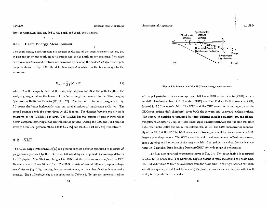
Figure 3.3: A quadrant schematic view of the SLD.
(a) (b)
Figure 3.4: SLD coordinate system.
Tracking devices
CCD Vertex Detector barrel
Central Drift Chamber
Endcap Drift Chambers
Particle identification devices
Cherenkov Ring Imaging Detector
Calorimeters
barrel
endcap
barrel and endcap
Liquid Argon Calorimeter barrel and endcap
Warm Iron Calorimeter barrel and endcap i
Luminosity Monitor and Small Angle Tagger endcap
Medium Angle Silicon Calorimeter endcap
Magnet barrel
Table 3.2: SLD subsystems.
26 27
3.2 SLD Experimental Apparatus
(25 mm rad)
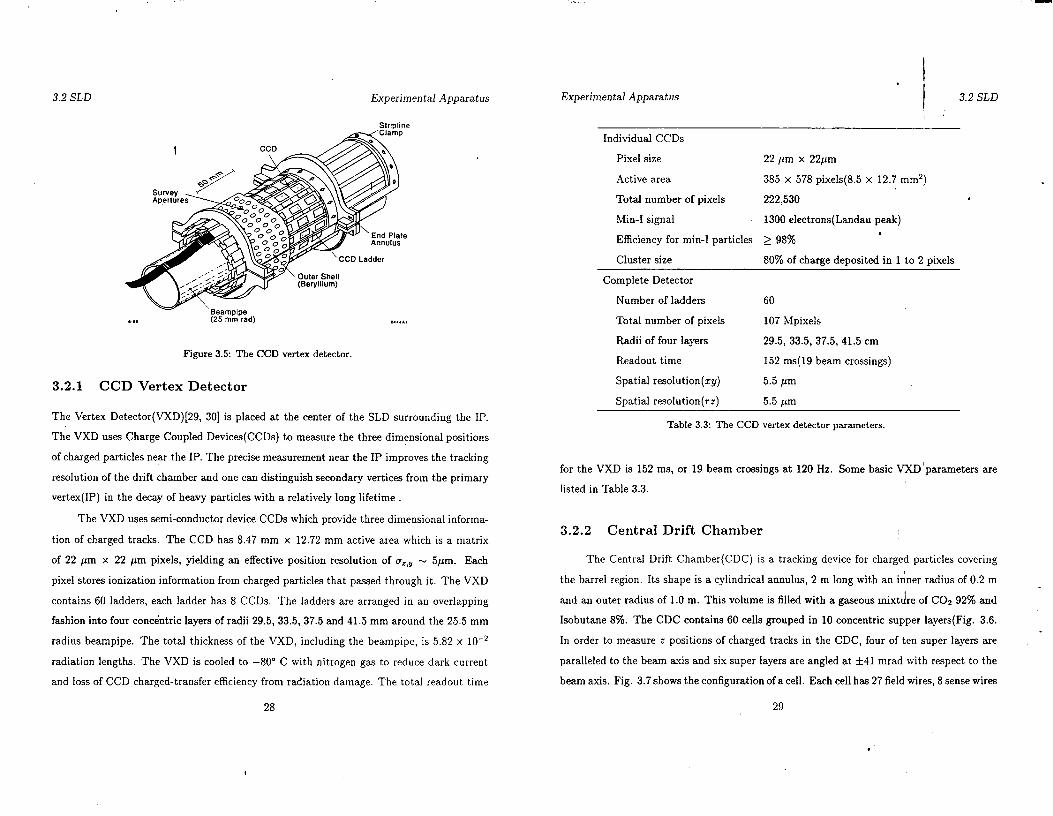
Figure 3.5: The CCD vertex detector.
3.2.1 CCD Vertex Detector
The Vertex Detector(VXD)[29, 301 is placed at the center of the SLD surrounding the IP.
The VXD uses Charge Coupled Devices(CCDs) to measure the three dimensional positions
of charged particles near the IP. The precise measurement near the IP improves the tracking
resolution of the drift chamber and one can distinguish secondary vertices from the primary
vertex(IP) in the decay of heavy particles with a relatively long lifetime .
The VXD uses semi-conductor device CCDs which provide three dimensional informa-
tion of charged tracks. The CCD has 8.47 mm x 12.72 mm active area which is a matrix
of 22 pm x 22 pm pixels, yielding an effective position resolution of a,,, N 5pm. Each
pixel stores ionization information from charged particles that passed through it. The VXD
contains 60 ladders, each ladder has 8 CCDs. The ladders are arranged in an overlapping
fashion into four concdntric layers of radii 29.5, 33.5, 37.5 and 41.5 mm around the 25.5 mm
radius beampipe. The total thickness of the VXD, including the beampipe, is 5.82 x lo-*
radiation lengths. The VXD is cooled to -80” C with nitrogen gas to reduce dark current
and loss of CCD charged-transfer efficiency from radiation damage. The total readout time
28
Experimental Apparatus . I
3.2 SLD
Individual CCDs
Pixel size 22 pm x 22pm
Active area 385 x 578 pixels(8.5 x 12.7 mm2)
Total number of pixels 222,530
Min-I signal 1300 electrons(Landau peak)
Efficiency for min-I particles 2 98% .
Cluster size 80% of charge deposited in 1 to 2 pixels
Complete Detector
Number of ladders
Total number of pixels
Radii of four layers
Readout time
Spatial resolution(q)
Spatial resolution(rz)
60
107 Mpixels
29.5, 33.5, 37.5, 41.5 cm
152 ms(19 beam crossings)
5.5 pm
5.5 firn
Table 3.3: The CCD vertex detector parameters
for the VXD is 152 ms, or 19 beam crossings at 120 Hz. Some basic VXD’parameters are
listed in Table 3.3.
3.2.2 Central Drift Chamber
The Central Drift Chamber(CDC) IS a tracking device for charged particles covering
the barrel region. Its shape is a cylindrical annulus, 2 m long with an iiner radius of 0.2 m
and an outer radius of 1.0 m. This volume is filled with a gaseous mix&e of CO2 92% and
Isobutane 8%. The CDC contains 60 cells grouped in 10 concentric supper layers(Fig. 3.6.
In order to measure z positions of charged tracks in the CDC, four of ten super layers are
paralleled to the beam axis and six super layers are angled at *41 mrad with respect to the
beam axis. Fig. 3.7 shows the configuration of a cell. Each cell has 27 field wires, 8 sense wires
29
:
3.2 SLD Experimental Apparatus
Figure 3.6: CDC superlayers.
Experimental Apparatus
I 1 3.2 SLD
Inner/outer radius
Length
Innermost/outermost wire layer radius
Wire length
Number of superlayers
Number of axial/stereo superlayen
Number of cells
Number of sense wires per cell
Stereo angle
Sense wire diameter (tungsten)
Field wire diameter (Cu-Be)
Guard wire diameter (Cu-Be)
Average drift field
GX3
Average drift velocity
Amount of material:
Inner wall
Wires
GlS
Outer wall
End plates and electronics
ZOO/l000 mm
2000 mm
238/961 mm
1800 mm
10
416
640
8
* 41 mrad
25 pm
152 pm
152 pm
0.13 kV/mm
COs 92%-Isobutane 8%
9 pm/ns
0.009 x,
0.020 x, :
0.006 x,
0.018 X0 1
0.20 x0 I
Table 3.4: The CDC parameters.
Figure 3.7: Detail of a CDC cell. l represents a sense wire. + and x represent a guard wire
and a field wire, respectively.
30
3.2 SLD Experimental Apparatus Experimental Apparatus
and 24 guard wires. The sense wires are made of tungsten, 25 pm radius and the resistance
is 300 0. The field and gua;rd wires are made of Cu-Be with 152 pm radius. The guard wires
are surrounding the sense wires to shape electric fields. High voltages are applied to the field
and guard wires to make electric fields. The charged particle passing through a cell creates
electrons liberated by ionizing the gas. The liberated electrons drift in the electric field(0.13
kV/mm) towards sense wires at a constant velocity of 9 pm/ns. Near the sense wires, they
are accelerated by the fields and make avalanches of - lo5 electrons which are detected by
the sense wires. The zy position is calculated from the drift t ime under the assumption
of constant drift velocity. The spatial resolution(in zy) for each wire is approximately 100
pm. The signal is read out at both ends to measure the z position by charge division. The
measurement error of z position is approximately fl m m in reconstruction of tracks. The
momentum of the charged particle is determined by the hit information along the particle
trajectory. In the barrel region, momentum resolution is formulated by
h4 - P
0.012 + (0.0025~)~. (3.2)
Using the CCD hit constraint, momentum resolution is improved to
4 - P
Jo.012 + (O.O015p)2. (3.3)
The basic CDC parameters are summarized in Table 3.4.
3.2.3 Endcap Drift Chambers
At angles of less than 30” with respect to the beam axis, the tracking resolution and efficiency
of the CDC degrades drastically since the tracks only pass through a fraction of CDC layers.
The endcap drift chambers track charged particles in the forward and backward regions
between 12” and 40”. The EDC consists of two sets of drift chambers, inner and outer,
in both endcaps, placed at z = f1.2 m and = 62.0 m. Each of four drift chambers has
three superlayers with a relative rotation 60”. The inner- and outer-chamber superlayers
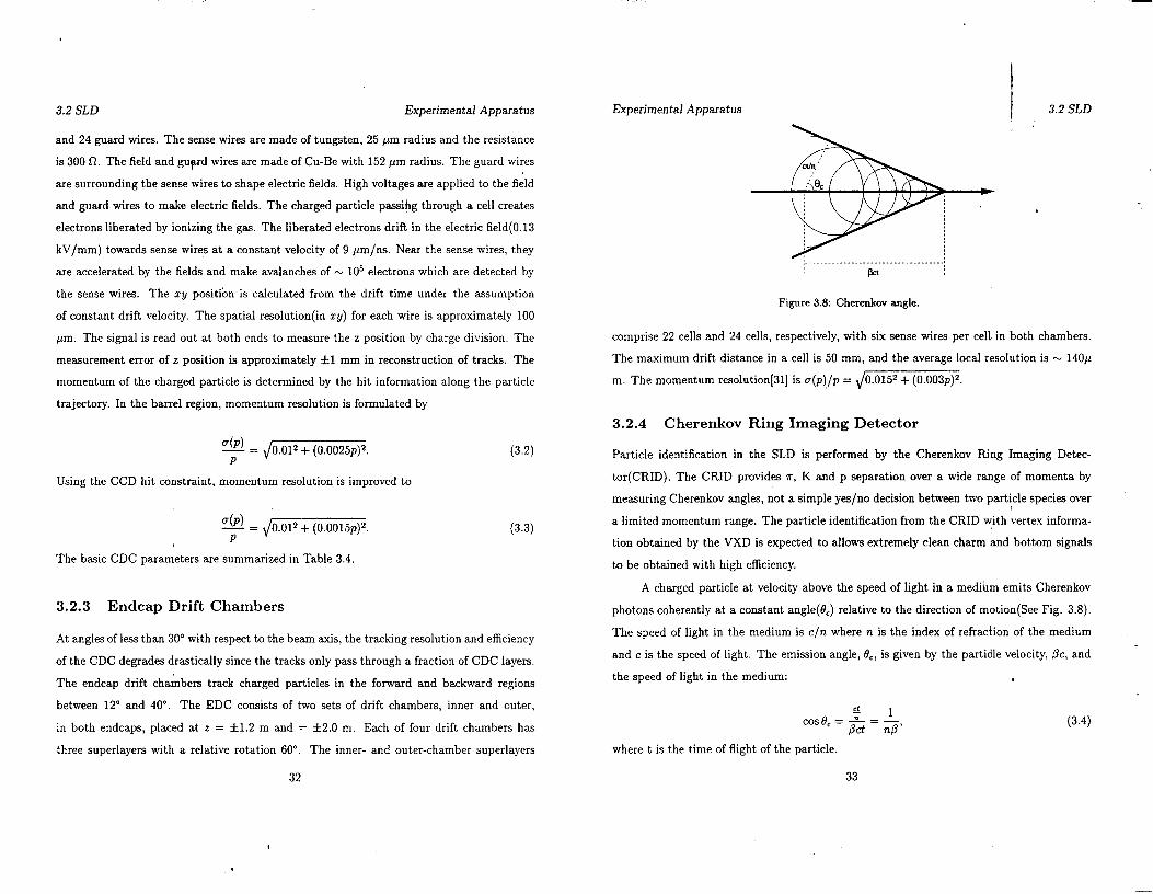
A charged particle at velocity above the speed of light in a medium emits Cherenkov
photons coherently at a constant angle(0,) relative to the direction of motion(See Fig. 3.8).
The speed of light in the medium is c/n where n is the index of refraction of the medium
and c is the speed of light. The emission angle, 0,, is given by the partidle velocity, PC, and
the speed of light in the medium: a
where t is the time of flight of the particle.
32 33
I I 3.2 SLD ; :
Figure 3.8: Cherenkov angle.
comprise 22 cells and 24 cells, respectively, with six sense wires per cell in both chambers.
The maximum drift distance in a cell is 50 mm, and the average local resolution is - 140~
m. The momentum resolution[31] is a(p),/p = \/O.O152 + (0.003~)~.
3.2.4 Cherenkov Ring Imaging Detector
Particle identification in the SLD is performed by the Cherenkov Ring Imaging Detec-
tor(CRID). The CRID provides rr, K and p separation over a wide range of momenta by
measuring Cherenkov angles, not a simple yes/no decision between two particle species over
a limited momentum range. The particle identification from the CRID with vertex informa-
tion obtained by the VXD is expected to allows extremely clean charm and bottom signals
to be obtained with high efficiency.
3.2 SLD Experimental Apparatus
Liquid Radiator /
(Cs FM) /
Figure 3.9: Schematic view of the barrel GRID.
A cross-section view of the barrel CRID is shown in Fig. 3.9. The barrel CRID consists
of liquid radiators, drift boxes, gas radiators and mirrors. In Fig. 3.9, a charged particle
passes through the CRID and produces Cherenkov lights in both liquid and gas radiator.
The Cherenkov light emitted in the liquid radiator enters the drift box directly while the
light produced in the gas radiator is focused back onto the drift box by spherical mirrors
and forms a sharp image. The number of transmitted photons is IO-20 for both radiators.
The drift box is filled with a gaseous mixture of CzHs and 0.1% TMAE(Tetrakis Dimethyl
Amino Ethylene). The photons from the both radiators pass through quartz windows on
the front and back of the detector box and are converted to electrons by photo-ionization
gaseous TMAE, which has a very high quantum efficiency in the wavelength range from li0
nm to 220 nm. The drift box is surrounded by a field cage. shown in Fig. 3.9. lvhich provides
a uniform electric field along z direction. The electrons are drifted by the electric field at
constant velocity towards anode sense wires. Near the sense wires, they are accelerated, make
avalanches of electrons before reaching anode. Three coordinates of the point of origin of
photoelectron are measured as the drift time of the electron, the wire address and conversion
34
Experimental Apparatus
I . 1 i .’ 3.2 SLD
Figure 3.10: Schematic of the CFUD drift box.
depth, which is determined by charge division(see Fig. 3.10). The basic parameters of the
CRID are summarized in Table 3.5.
3.2.5 Liquid Argon Calorimeter
The measurement of energies of particles is done by the Liquid Argon Calorimeter(LAC).
The LAC was designed to have excellent energy resolution both for electromagnetic and
hadronic particles and to be fully hermetic. For this purpose, the LAC yas placed inside the
magnet coil to avoid degrading the performance of the calorimeter due to energy absorption
in the material of the coil. The LAC consists of barrel and endcap, each section has two
electro-magnetic layers(EMl,EM2) and two hadronic layers(HADl,HADZ). The shape of
the barrel LAC is 6 m-long cylinder annulus with an inner radius of 2 m and an outer radius
of3m.
The LAC is made of stacks of lead tiles interspersed by gaps filled with liquid ar-
gon(cel1). Each cell is composed of a liquid argon ionization chamber, located between
parallel lead electrodes, held apart by plastic spacers(Fig. 3.11, 3.12). The tiles are alter-
35
.

3.2 SLD Experimental Apparatus Experimental Apparatus
I Liauid G&S
Radiator Material
Index of refraction
Thickness of radiator
Cherenkov angle (p = 1)
Radius of cherenkov ring (p = 1)
Number of photoelectrons (p = 1)
Momentum threshold
e
7r
K
P
W14
1.277
1 cm
672 mrad
17cm
14
CSF12
1.001725
-45cm
59 mrad
2.9 cm
14
1 MeV/c 9.5 MeV/c
0.23 GeVJc 2.6 GeV/c’
0.80 GeV/c 9.1 GeV/c
1.50 GeV/c 17.3 GeV/c
Table 3.5: The barrel CRID parameters.
Load bearing spacer columns, location of stainless steel bands.
I i .’ 3.2 SLD
Figure 3.12: Schematic of LAC.
Figure 3.11: Schematic of LAC segment
36 37

3.2 SLD Experimental Apparatus
Figure 3.13: Schematic of the WIC layers.
nately at ground potential and at negative high voltage. Lead is used as absorber as well as
electrodes. The LAC measures ionization in the liquid argon which is proportional to the
energy loss of the incident particle. Therefore the energy of the particle is calculated from
the collected charge. The resolution of energy measurement of the E M section is
4E) 0.08 E =7F
That of HAD section is
4E) 0.55 -=- E dE
(3.5)
(3.6)
. 3.2.6 Warm Iron Calorimeter
The Warm Iron Calorimeter(WIC) is the outer structure of the SLD, consisting of a barrel
part and two endcap parts. The barrel part is divided into eight sections, which are 6.75 m
long and 1.18 m thick. The WIC has three purposes : The first use is to absorb and measure
the leakage of the hadronic showers from the LAC. The second is to identify muons. Finally,
38
Experimental Apparatus i .’ 3.2 SLD
lb
z-94 MASC LMSAT 7-W
Figure 3.14: Schematic of the LUM.
the WIC serves as a flux return for the 0.6 T solenoidal magnetic field. The structure of
the WIC is segmented into 14 layers, 50 m m thick iron with 32 m m gaps instrumented with
streamer tubes as shown in Fig. 3.13. The tubes are made of the graphite coated plastic 9
m m x 9 m m tubes(1 m m thick) with 100 pm diameter Be-Cu wires. The tubes are filled
with a gas mixture of 88% carbon dioxide, 9.5% isobutane and 2.5% argon and 4.75 kV high
voltage is applied to the wires. On the top and bottom of the tubes, there are stripes of GlO
plated with copper patterns in shapes of strips and pads. Charged particles create streamer
discharges in the tubes, which induce signals on the strips and pads. The’strips run parallel
to the tubes to track muons. The pads are segmented so that they continue the projective
tower geometry of the LAC to measure the shower energies. Fourteen layers of iron and
streamer tubes are divided into two radial layers. The seventh and fou it eenth layers are
double layer chambers to give two-dimensional position information for muon tracking.
3.2.7 Luminosity Monitor
39
3.2 SLD Experimental Apparatus
The Luminosity Monitor and Small Angle Tagger(LMSAT) and the Medium Angle Silicon
Calorimeter(MASiC) me&sure electromagnetic showers in the 23-190 mrad region of 8. This
measurement determines the integrated luminosity of the SLD by detecting Bhabha (e+e- +
e+e-) events. The cross section for this process, dominated by the plhoton exchange t-channel
process, has been calculated with high precision. The LMSAT and MASiC are located
on both sides of the IP. They are cones of silicon detector centered around the beampipe
with a projective tower structure like the LAC. The LMSAT, a silicon-tungsten sampling
calorimeter, covers the angles from 23 to 68 mrad at a distance of 1 m from the IP. It consists
of 23 tungsten plates of 3.5 mm thickness, spaced 4.5 mm apart, for a total of 21 radiation
lengths. Like the electromagnetic part of the LAC, the LMSAT is split up in EMl(first 6
layers) and EMZ(remaining 17 layers). The MASC, lying at 31 cm from the IP and covering
from 68 to 190 mrad, consists of ten 6.6 mm thick tungsten and is split up in EM1 and EM2.
The energy resolution of the LMSAT is 23%/G and the angular resolution is &3 = 0.3
mrad and &J = 6.5 mrad, which are adequate to measure Bhabha events.
3.2.8 Magnetic Coil
The magnet, located between the LAC and the WIC, is a 5.9 m diameter and 6.4 m long
normal coil made of aluminum cooled by water. A magnetic field of 0.60 T in the center
of the coil is provided by a current of 6600 A through 508 turns. The steel in the barrel
and endcap WIC provides the return flux path for the magnetic field. The radial and z
components of the magnetic field are given by
B, = B,oz To*0
T2 - 2Z2 B, = B,” +0.58,0-
To20 (3.7)
where B,” = O.O214T, B,” = 0.60lT, TO = 1.2m and zs = 1.5m agrees with measured field to
with 0.05% inside the CDC and to within 0.4% for the EDC. The uniformity of the field is
more than adequate for the momentum measurements.
40
Experimental Apparatus D Monte Carlo
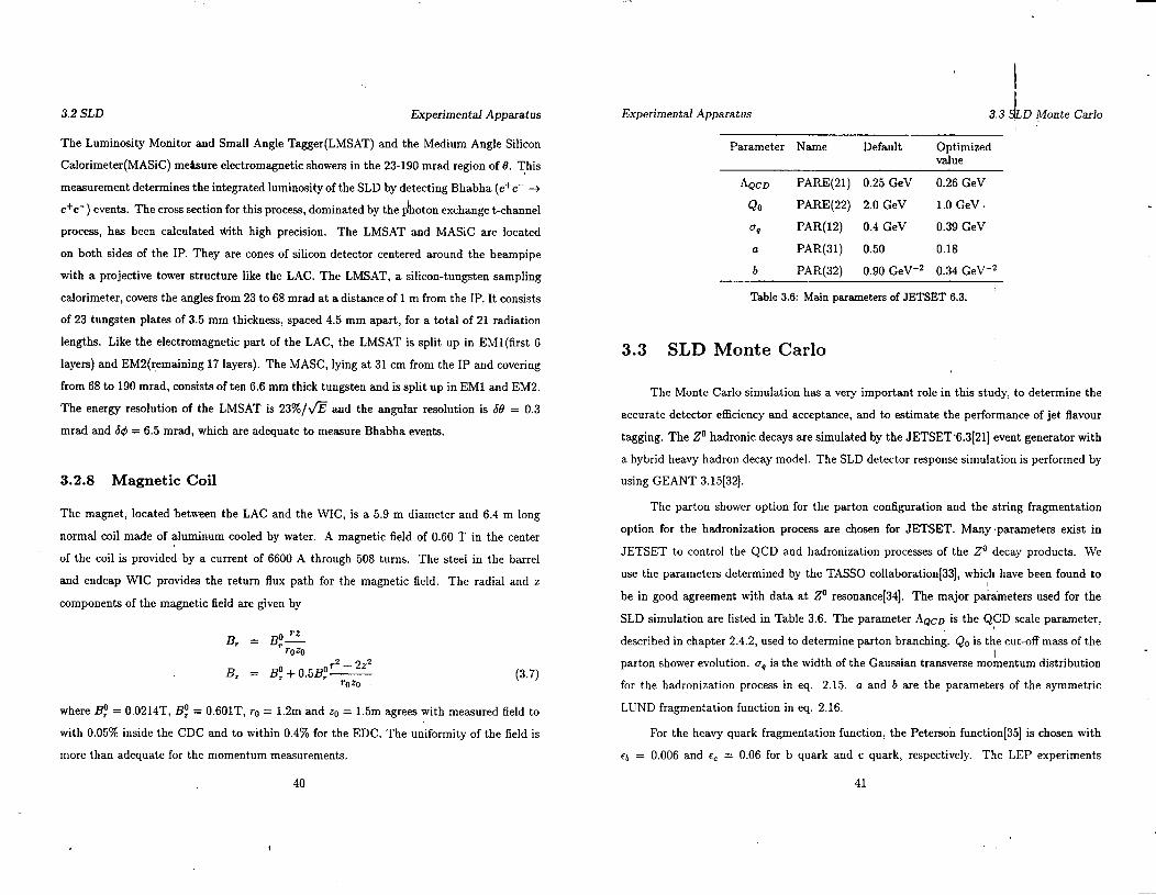
Parameter Name Default Optimized value
AQCD PARE(21) 0.25 GeV 0.26 GeV
Qo PARE(22) 2.0 GeV 1.0 GeV
UP PAR(12) 0.4 GeV 0.39 GeV
a PAR(31) 0.50 0.18
b PAR(32) 0.90 GeVb2 0.34 GeV2
Table 3.6: Main pararreters of JETSET 6.3.
3.3 SLD Monte Carlo
The Monte Carlo simulation has a very important role in this study, to determine the
accurate detector efficiency and acceptance, and to estimate the performance of jet flavour
tagging. The Z” hadronic decays are simulated by the JETSET.6.3[21] event generator with
a hybrid heavy hadron decay model. The SLD detector response simulation is performed by
using GEANT 3.15[32].
The parton shower option for the parton configuration and the string fragmentation
option for the hadronization process are chosen for JETSET. Many aparameters exist in
JETSET to control the QCD and hadronization processes of the Z” decay products. We
use the parameters determined by the TASS0 collaboration[33], which have been found to
be in good agreement with data at Z” resonance[34]. The major parameters used for the
SLD simulation are listed in Table 3.6. The parameter hQc~ is the QCD scale parameter,
described in chapter 2.4.2, used to determine parton branching. Qe is the cut-off maas of the I
parton shower evolution. eq is the width of the Gaussian transverse momentum distribution
for the hadronization process in eq. 2.15. a and b are the parameters of the symmetric
LUND fragmentation function in eq. 2.16.
For the heavy quark fragmentation function, the Peterson function[35] is chosen with
E* = 0.006 and E, = 0.06 for b quark and c quark, respectively. The LEP experiments
41
3.3 SLD Monte Carlo Experimental Apparatus Experimental Apparatus I
3.3 SLJj MoDte Carlo
I
Particles from B decay (N) ov Monte Carlo Measurements
e 0.110 0.104 f 0.004[8]
P 0.110 0.103 f 0.005[?]
I- 0.030 0.041 f O.OlO[S]
DO 0.629 0.621 f 0.026[42]
D+ 0.259 0.239 f 0.037[42]
DS 0.099 0.100 f 0.025[42]
D*+ 0.236 0.230 f 0.040[8]
Charmed baryon 0.060 0.064 f 0.011[8]
J/G 0.014 0.013 f 0.002[8]
D(‘)Ds’) 0.065 0.050 f 0.009[8]
n*(direct) 3.564 3.59 f 0.11[43]
K* 0.765 0.78 f 0.04[43]
K0 0.692 0.64 f 0.04[43]
P 0.092 0.080 f 0.005[8]
A 0.023 0.040 f 0.005[8]
Table 3.7: Average numbers of particles from B, and & mesons’ decay.
have found that the M.C. simulation with those parameters reproduces the experimental
data[36] well including the average total charged multiplicity of Z” hadronic events[37]. To
be consistent with recent measurements of B meson decays, the M.C. parameters are tuned
as follows[38]:
l Semileptonic decay
The ISGW[39] form factor model is used for the semileptonic B meson decays. The
branching fractions to e, p and 7 are set to 0.11, 0.11 and 0.03, respectively. D,
D' and D" production fractions in the semileptonic decays are set to 0.33, 0.58 and
0.09, respectively. A total semileptonic decay branching fraction is 25%. The lepton
momentum spectra from I?, and B,j with these parameters give good agreement with
the recent CLEO data[rlO].
l Hadronic two body decay
A total of 12.5% of the B meson branching fraction is set to the hadronic two body
decays tabulated by the Particle Data Group[b].
l Baryon production
A total of 6% is set to the charm baryon productions based on the CLEO measurement[41].
The remaining 56.5% of the branching fraction is attributed to the inclusive particle
production fractions by using the modified JETSET heavy hadron decay backage. Table 3.7
shows the comparison of the average number of particles produced by B, and Bd decays
between the data and the Monte Carlo simulation, and is indicating good agreement with
data. I
The detector simulation of the SLD is performed by GEANT 3.15, which provides
the detector response to charged and neutial particles produced by the event generator.
GEANT swims particles inside the SLD from the IP, according to particle momentum and
the magnetic field with a geometric description of the SLD. During the swimming, multiple
scattering, energy loss of the charged particle, nuclear interaction’with the detector material,
43 42
3.4 SLD Event Reconstruction Experimental Apparatus
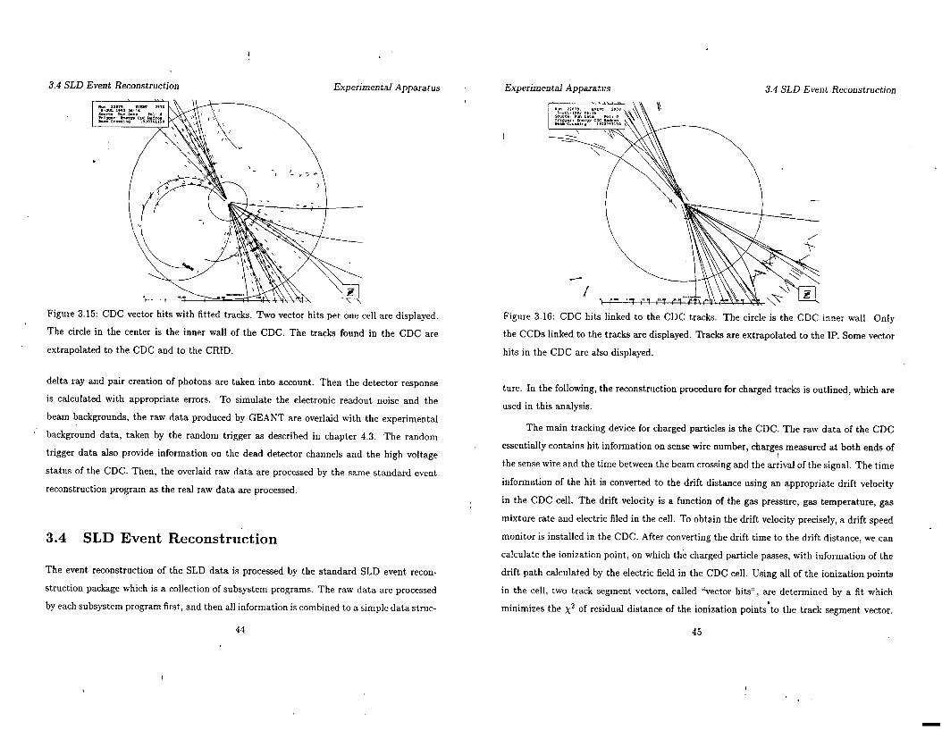
Figure 3.15: CDC vector hits with fitted tracks. Two vector hits per one cell are displayed.
The circle in the center is the inner wall of the CDC. The tracks found in the CDC are
extrapolated to the CDC and to the CRID.
delta ray and pair creation of photons are taken into account. Then the detector response
is calculated with appropriate errors. To simulate the electronic readout noise and the
beam backgrounds, the raw data produced by GEANT are overlaid with the experimental
(’ background data, taken by the random trigger as described in chapter 4.3. The random
trigger data also provide information on the dead detector channels and the high voltage
status of the CDC. Then, the overlaid raw data are processed by the same standard event
reconstruction program as the real raw data are processed.
3.4 SLD Event Reconstruction
The event reconstruction of the SLD data is processed by the standard SLD event recon-
struction package which is a collection of subsystem programs. The raw data are processed
by each subsystem program first, and then all information is combined to a simple data struc-
44
Experimental Apparatus 3.4 SLD Event Reconstruction
Figure 3.16: CDC hits linked to the CDC tracks. The circle is the CDC inner wall. Only
the CCDs linked to the tracks are displayed. Tracks are extrapolated to the IP. Some vector
hits in the CDC are also displayed.
ture. In the following, the reconstruction procedure for charged tracks is outlined, which are
used in this analysis.
The main tracking device for charged particles is the CDC. The raw data of the CDC
essentially contains hit information on sense wire number, charges measured at both ends of
the sense wire and the time between the beam crossing and the arrival of the signal. The time
information of the hit is converted to the drift distance using an appropriate drift velocity
in the CDC cell. The drift velocity is a function of the gas pressure, gas temperature, gas
mixture rate and electric filed in the cell. To obtain the drift velocity precisely, a drift speed
monitor is installed in the CDC. After converting the drift t ime to the drift distance, we can
calculate the ionization point, on which the charged particle passes, with information of the
drift path calculated by the electric field in the CDC cell. Using all of the ionization points
in the cell, two track segment vectors, called “vector hits”, are determined by a fit which
minimizes the x2 of residual distance of the ionization points’to the track segment vector.
45
3.4 SLD Event Reconstruction Experimental Apparatus
We have two vector hits because it is not possible to determine on which side electrons are
drifted to the sense wires. T&s left-right ambiguity is solved by the pattern recognition with a
vector hits in superlayers. The CDC pattern recognition program(441 i ‘r also used to combine
- vector hits into the track(Fig. 3.15). Then, the track found in the CDC is tried to link to the
CCD vertex detector hits to form a complete tra.ck(Fig. 3.16). Finally, the track is fitted to
a helix trajectory, which gives the information of the charge and momentum of the charged
particle associated with the track. The information of charge and momentum of the tracks
is written to the Data Summary Tape(DST).
46
Chapter 4
Event Selection
In this chapter, we describe the 2’ hadronic event selection procedure. The hadronic
event selection is made in three stages. The first is an online event trigger. The second is
an offline filter designed to select Z” hadronic and leptonic decay’events. In the final stage,
we select hadronic events in offline analysis.
We obtain w 45,000 hadronic events through those stages from the data collected by
the SLD in 1992 and 1993 runs.
Before describing the hadronic event selection, we will review the properties of the data
taking and summarize event topologies of Z” decays and physics background event.
4.1 Data Taking
In 1991, SLD data taking started with the engineering run. The electroh beams were not
polarized at that time. During three months, about 400 Z” decays were collected. The 1992
run began in June and ended in December with f22% polarized electron beams. About
10,000 Z”s were collected. In 1993, the run was started in March and ended in August. Dur-
ing those five months, about 50,000 Z” decays were collected with f63% polarized electron
beams. The electron polarization was improved by a newly-developed strained-lattice GaAs
47

4.2 El ient Top< Event Selection
Figure 4.1: A hadronic event candidate with 4-jet event shape. From the center, CDC,
CRID, LAC, Magnet and WIC are displayed. Charged tracks reconstructed by the CDC
are, shown as white curves, extrapolated to outside of the CDC. Towers in the LAC and
WIC represent amounts of energy deposits.
photocathode.
In this analysis, we use the data of 1992 and 1993. The data of 1991 was taken by
different detector configuration and was not used for this analysis.
4.2 Event Topologies
The following are the event topologies considered for this study:
1. Z” hadronic decays(ZO + Jf -r hadrons)
70% of Z” decays are into hadrons. The charged multiplicity of a hadronic decay is
large(- 20 average), and a large amount of energy is deposited in the calorimeters.
The total momentum of the event is well balanced. A hadronic event candidate with
4-jet event shape is shown in Fig. 4.1.
48
Event Selection
I J 4.2 E ,ent Topologies I .’
Figure 4.2: A wide angle ahabha event candidate. Two back-to-back charged tracks, shown
as white lines, are detected by the CDC(centra1 black circle). They deposit all of their
energies in the EM section of the LAC. Other energy deposits in the LAC are considered as
beam related backgrounds.
49
4.3 Event Trigger Event Selection Event Selection
e+
Figure 4.5: Feynman diagram of a two-photon process and a 7-7 process
4.3 Event Trigger
The SLD trigger[45,46] is designed to record Z” events efficiently, while vetoing beam related
background as much as possible. In order to decide whether to accept or veto an event, either
tracking devices(the CDC and the WIC) or calorimetry(the LUM and the LAC) are used.
The trigger decision time is -4 msec and typical readout time for the entire detector is about
200 msec. Typical trigger rates were 0.5 - 2 Hz, depending on the beam conditions. There
are seven different triggers to record several kind of physics events on tape.
1. Energy
The sum of energy deposits in the barrel and endcap LAC above thresholds is greater
than 4 GeV, where the thresholds for the EM and HAD section are 154 MeV and 811
MeV, respectively. Only calorimetry information is read out by this trigger.
2. LUM
The sum of energy deposits for each LUM EM2 section above threshold is greater than
12.5 GeV, where the threshold is 1.25 GeV. Calorimetry information is read out.
52
I . 4. Oftline Filter
3. WAB
The sum of energy deposits in the LAC EM section above threshold is 15 GeV, where
threshold is 154 MeV. All subsystems are read out by this trigger.
4. Tracking
Followings are required for this trigger:
(a) at least two CDC tracks,
(b) opening angle of two tracks > 30”,
(c) trigger rate < 0.1 Hz.
All subsystems are read out.
5. Hadronic
There is at least one CDC tracks, and the energy trigger is satisfied. All subsystems
are read out
6. Muon
There are two back-to-back barrel WIC tracks. All subsystems are read out.
7. Random
This is triggered every 2,400 beam crossings(20 sec.). All subsysterps are read out
The energy thresholds shown above were changed several times. The actual readout
thresholds for the data analysis are much lower(5/8/41/41 MeV for EMl/EMB/HADl/HAD2)
A CDC track is defined to have at least nine superlayer hits in the CDC, &here the superlayer
hit is defined to have at least 6 sense wire hits in a superlayer. A WIC track is defined to
have at least 4 hits. The data taken by the Random trigger is used for background studies. I
4.4 Offline Filter
This stage is needed to select good candidates of Z” hadronic decays and charged lepton
pairs(e+e-,C1+~-,7+7-) from the triggered events. To select hadronic decays. the following
53
4.5 Hadronic Event Selection Event Selection Event Selection
criteria are required to be satisfied:
I 1. The total energy deposit in the barrel and endcap LAC is greater than 14 GeV. ’
2. The energy deposit in the endcap WIC < 11 GeV. This cut removes SLC muon back-
grounds produced at up stream of the beams.
3. Eimb. < 0.9 and (Eimb. + S) < 1, where S is the sphericity[47] and Eimb. is the energy
imbalance defined as ,
Eima = E hcm1 - Ehcmz &ml •!- Ehemz’
(4.1)
Ehc,,,l and Ehc,,,Z are the energy deposits in the two hemispheres divided by the plane
perpendicular to the sphericity axis. The sphericity S is defined by
CP?T S=zmin i ( 1 TP? (4.2)
where subscript T denotes transverse momentum to the axis, called sphericity axis,
which minimizesthe sum in the numerator. The sphericity lies in the range 0 5 S 5 1.
Events with S z 1 are rather spherical and events with S z 0 look like a back-to-back
P-jet.
To identify p/i, a pair of WIC strip tracks are required to be roughly back-to-back. A
of event is required to have at least one CDC good track with momentum greater than 1
GeV.
4.5 Hadronic Event Selection
The events passing the offline filter are fully reconstructed and written to data summary
tapes. To select the events suitable for this analysis, we define good tracks first. Then good
hadronic events are selected using the good tracks. The good tracks are selected by requiring
54
4.5 Hadronic ! E ,ent Selection I
+ Data
JL MonteCarlo
0 L 111’11”111’(11’11”111’111’111 ‘8 1 -1 -0.8 -0.6 -0.4 -0.2 0 0.2 0.4 0.6 0.8 1
case
Figure 4.6: cos0 distribution of charged tracks. Data and M.C. are normalized in the range
1 cos&,cliI < 0.8.
0.2 P-- I 0 ~-‘,‘,,“‘,,“““,“,,,““,‘,,,,‘,,‘,’,,’,I’,,,1
0 0.1 0.2 0.3 0.4 0.5 0.6 0.7
Figure 4.7: Pt distribution of charged tracks. Data and M.C. are normalized in the range
Pt > 0.15.
55
4.5 Hadronic Event Selection Event Selection
z 0.09 2 z
0.08 -0 0.07 z 3 0.06
0.05 0.04 0.03 0.02 0.01
0
Multiplicity
Figure 4.8: Charged multiplicity(n&) distribution of Z” hadronic decay candidates. Data
and M.C. are normalized in the range n,h 2 5.
-2 0.05 t >
~0.04 -
Y-
z + Data
JL MonteCarlo
Figure 4.9: Visible energy(E,iS) distribution of 2’ hadronic decay candidates. Data and
M.C. are normalized in the range E,,, > 0.2E,.
56 57
Event Selection 4.5 Hadronic & vent Selection ; .’
g 1 aI- ;; 0 0.8
2 6 0.6
5 0.4
0.2
0 ~.,,,l,,,l,,,,,,‘,,,,,,,,,‘,,‘,,’I,. J -1 -0.8 -0.6 -0.4 -0.2 0 0.2 0.4 0.6 0.8 1 -
cwhst
1
+ Data
n MonteCarlo
Figure 4.10: cos &hrust distribution of Z” hadronic decay candidates. Data and M.C. are
normalized in the range 1 cos &hrurfI < 0.7.
1. ) cosBtrooCl < 0.8,
2. A transverse momentum(&) greater than 0.15 GeV/c,
3. R < 5 cm,
4. IzI < 10 cm.
Due to limited CDC coverage in polar angle, cut 1 is required. In Fig. 4.6, cosBtraek dis-
tributions of the data and the M.C. are shown. In the central region, the M.C. reproduces
the distribution of data well. Outside the coverage of the CDC(l cos6( ? 0.8), the track re-
construction efficiency drops off, and the M.C. simulation slightly overestimates the tracking I
efficiency. Thus cos 0 = f0.8 is chosen to remove tracks which are poorly measured and are
not simulated by the M.C. well. The Pt distributions of charged tracks is shdwn in Fig. 4.7.
In the low Pr region, the M.C. simulation is different from the data which has slightly softer
Pl spectrum. This is due to the difficulty of simulating multiple scattering of low momentum
tracks. Pt > 0.15 GeV/c is chosen to ensure consistency between data and M.C. These low
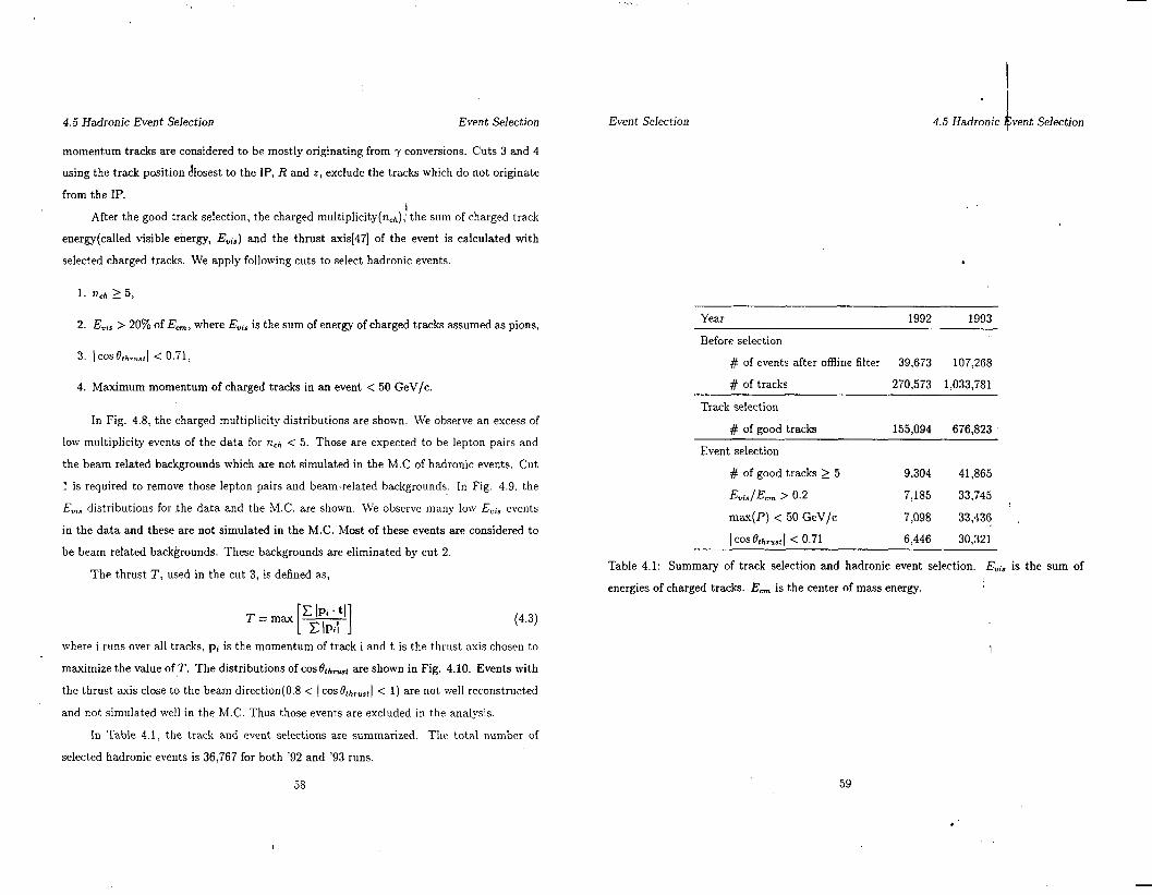
-.
4.5 Hadronic Event Selection Event Selection Event Selection
momentum tracks are considered to be mostly originating from y conversions. Cuts 3 and 4
using the track position Closest to the IP, R and z, exclude the tracks which do not originate
from the IP.
After the good track selection, the charged multiplicity(n&,),’ the sum of charged track
energy(called visible energy, E”is) and the thrust axis[47] of the event is calculated with
selected charged tracks. We apply following cuts to select hadronic events.
2. Eeis > 20% of E,, where Euis is the sum of energy of charged tracks assumed as pions,
3. ) CoS&.us~l < 0.71,
4. Maximum momentum of charged tracks in an event < 50 GeV/c.
In Fig. 4.8, the charged multiplicity distributions are shown. We observe an excess of
low multiplicity events of the data for nch < 5. Those are expected to be lepton pairs and
the beam related backgrounds which are not simulated in the M.C of hadronic events. Cut
1 is required to remove those lepton pairs and beam-related backgrounds. In Fig. 4.9, the
E,,,, distributions for the data and the M.C. are shown. We observe many low EDis events
in the data and these are not simulated in the M.C. Most of these events are considered to
be beam related backgrounds. These backgrounds are eliminated by cut 2.
The thrust T: used in the cut 3, is defined as,
C IPi tl T=max ___ [ 1 C IPil (4.3)
where i runs over all tracks, pi is the momentum of track i and t is the thrust axis chosen to
maximize the value of T. The distributions of cos 6’ h t ru,* are shown in Fig. 4.10. Events with
the thrust axis close to the beam direction(0.8 < 1 cos8rhrustI < 1) are not well reconstructed
and not simulated well in the M.C. Thus those events are excluded in the analysis.
In Table 4.1, the track and event selections are summarized. The total number of
selected hadronic events is 36,767 for both ‘92 and ‘93 runs.
58
4.5 Hadronic vent Selection
Year 1992 1993
Before selection
# of events after offline filter 39,673 107,268
# of tracks 270,573 1,033,781
Track selection
# of good tracks 155,094 676,823
Event selection
# of good tracks 2 5 9,304 41,865
&is/Eon > 0.2 7,185 33,745
max(P) < 50 GeV/c 7,098 33,436
1 cos @thrust 1 < 0.71 6,446 30,321
Table 4.1: Summary of track selection and hadronic event selection. E”is is the sum of
energies of charged tracks. E, is the center of mass energy.
59

4.6 Background Estimation
4.6 Background Estimation
Event Selection
The major sources of b&kg rounds in the hadronic events selected in previous section .are
r+r- pairs, two photon processes and beam-related events. In this section, we estimate I
those background contaminations in our hadronic event samples. The total contamination
of backgrounds in the hadronic event sample is estimated to be less than 0.4%. This value
is considered to be negligible in this study because we apply more tight cuts for selecting
good J-jet events in this analysis. Thus, the background contaminations is not taken into
account in further analysis.
4.6.1 T+F Events
The main r decay mode is charged l-prong decay’ and its branching ratio is 85.5%(8]. The
branching ratio into charged 3-prongs is 14.4%. Table 4.2 summarizes expected charged
multiplicity of rf~- events. In the hadronic event selection, we require at least 5 charged
tracks in an event. This cuts out 97.7% of r+r- events naively. A more precise estimation of
r+r- event contamination can be done using a Monte Carlo simulation. The same selection
criteria as the hadronic Z” events are applied to a large number of generated M.C. r+r-
events. We have 4.20% f 0.13%[48] of the r+r- pairs which pass the cuts. This number
is larger than the naive expected value 2.3% due to additional charged tracks in a rfr-
event created by radiative photon conversions or interactions in the detector material. The
contamination of r+i- pairs is estimated to be 0.20% f 0.07% by multiplying by the ratio
BR(Z” + r+r-)/BR(Z’ + hadrons)= 4.7 %.
4.6.2 Two-Photon Processes
Event Selection I
4.6 Backgro 4
nd Estimation
T+T- decay mode r+r- decay charged multiplicity Ratio
l-prong & l-prong
l-prong & 3-prong
3-prong or more & J-prong or more
2 73.1 %
4 24.6 %
6 or more 2.3 %
Table 4.2: Summary of T+T- event multiplicity.
energy in the detector. As r+r- background estimation, two photon processes are simulated
by the M.C. It turns out that 0.5% f 0.1%[48] of two photon processes pass the hadronic
event selection cuts. The rate of two photon processes in hadronic event sample is therefore
estimated to be 0.10% f 0.03%.
4.6.3 Beam Related Events
The events caused by the interactions of the beam with the beam pipe wall or a nucleon
of a residual gas atom inside the beam pipe are called beam-related events. It is very hard
to calculate the cross sections for these events because they strongly depend on the beam
conditions which can vary over a short period of time. The contamination of these events
was estimated to be less than 0.1%[48].
The cross section for ,this process is estimated to be 6.5 nb[49] at fi = Ms, about one fifth
of the hadronic cross section. However, these events are not energetic enough to trigger the
detector. Most of events are very forward peaked and do not deposit a significant amount of
‘one charged and multiple neutral particles
60 61
4.6 Background Estimation
62
Event Selection
Chapter 5
Analysis
In this chapter, we make three samples of quark and gluon jets by jet flavour tagging
and compare them. First of all, using the Durham jet finding algorithm, we find 3-jet events
containing two quark jets(q and q) and one gluon jet. Then, we make three statistically
independent samples called the “gluon tagged” sample, the “light mixture” sample, and the
“heavy mixture” sample by jet flavour tagging of light quarks(u,d,s) and heavy quarks(c,b). ,
The gluon tagged sample is enriched with gluon jets. The light(heavy) mixture is the mixture
sample containing light(heavy) quark jets and gluon jets, These three samples have different
compositions of flavour and thus allow us to compare properties of quark and gluon jets.
In particular, we compare three jet properties:charged multiplicity, inclusjve energy fraction
and angular width. To unfold the pure state of light quark, heavy quark and gluon jet, we
use the M.C. to estimate the compositions of each jet sample. Only charged tracks are used
in this analysis. I
5.1 Three Jet Event Selection
63

k -

5.1 Three Jet Event Selection Analysis
In order to select J-jet events, we apply the kl(Durham) jet finder(501 to the selected hadronic
events. In each hadronic event, the quantity
yij E 2min(Ef,Ej)(l -COSt?ij)
EL 1 (5.1)
.
is calculated for all pairs of particles i and j, where Ei and Ej are the energies of two particles,
Bij is the opening angle between them, and Evis is the sum of the energies of all particles in
the event. We assume that all charged particles are pions in this analysis. Two particles(or
jets) i and j with the smallest Yij in the event are combined as a jet if yij is smaller than a
certain threshold value y,,,. The four-momentum of the combined jet is equal to the vector
sum of the constituent particles. This procedure is repeated until all y<j exceed Y~,,~. Fig.
5.1 shows the n-jet rates as a function of yut from data(symbols) and M.C. simulation(solid
lines). The number of found jets depends on y,,. At yeut = 0.003, the fraction of 3-jet events
is maximized. However, the fractions of 2-jet and 4 or more jet events change very much
around ycUt = 0.003. Therefore, the 3-jet event sample found around 0.003 includes 2-jet
or 4-jet like events which will be removed after the “well measured S-jet event selection”,
described later. To obtain the maximized fraction of “well measured 3-jet event”, we choose
ycut value 0.007.
After selecting J-jet events using the Durham jet-finder, we apply further cuts to obtain
well-measured events. Fig. 5.2 shows a schematic of a Q-jet event. The three arrows represent
the axes of the jets determined by the jet-finder. Ep is the sum of particle energies contained
in a jet. (Pi is the angle opposite to the jet i. The jets are ordered by jet energy(Ej+i) as
Ejet,l > Ejet,2 > Ejet.3. Ej,t,i is calculated in terms of E CM and the angles pi(Fig. 5.2) by
Ejet+ E ECM . sin pi
sin (PI + sin cpz + sin [p3
The following cubs are applied to obtain well-measured 3-jet events.
1. 1 COSBj,tl < 0.7,
where ejet is the polar angle of a jet. This is required for all 3 jets so that all jets are
contained in the sensitive barrel region of the CDC. In Fig. 5.3, the distributions of
66
Analysis 5.2 Flavour 1 agging of Jets
cos0jct are shown for the data and the M.C., representing that the jet reconstruction
efficiency drops at COS~~,~ > 0.i and cos6’jet < -0.7.
2. EVis > 5.0 GeV,
In Fig. 5.4, the E-is distributions are shown for the data and’ the M.C. A jet with low
visible energy is considered to be a low energy jet or a jet with large missing energy.
The error on the jet axis determination increases as &is gets smaller. Thus we require
that Evis of all jets in an event is greater than 5 GeV.
3. xvi > 358"y
e~pi is the sum of the angles between jets, and should be 360” if we measure all
p;rticles in an event perfectly because the Z” decays at rest. The deviation of the sum
of the angles from 360” in Fig. 5.5 is due to the effect of undetected neutral particles
and measurement error of charged track momenta. We exclude poorly measured events
which lie in the long tail in Fig. 5.5.
Fig. 5.6 shows a display of a typical 3-jet event which satisfies the 3-jet event selection
criteria. Table 5.1 summarizes the 3-jet events from the data and the M.C. obtained from this
selection. We obtain 5,693 good 3-jet events out of 36,767 hadronic events, corresponding
to 15.4% of the hadronic events.
5.2 Flavour Tagging of Jets
Flavour tagging of jets is based on the long lifetime of heavy quarks(b and c) and their large
boost in Z” decays due to the hard fragmentation functions. The average momentum of B
mesons produced by the 2’ decay is N 38 GeV/c and its average decay le:gth is - 2.2 mm.
Therefore, tracks from the heavy hadron decay typically have large impact parameters[SI]
and large transverse momenta relative to the initial hadron direction due to the large mass
of the heavy hadron. The impact parameter@) is defined as the closest approach of the
extrapolated track to the IP in the 2-y plane, as shown in Fig. 517. The IP used to measure
67
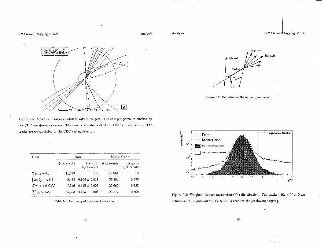
5.2 Flavour Tagging of Jets Analysis Analysis 5.2 FlavouriTaggjng of Jets
Figure 5.6: A hadronic event candidate with three jets. The charged particles tracked by
the CDC are shown as curves. The inner and outer wall of the CDC are also shown. The
tracks are extrapolated to the CDC vertex detector.
cuts Data Monte Carlo
# of events Ratio to # of events Ratio to 3-jet events 3-jet events
S-jet events 11,729 1.0 46,864
1 cosej,*I < 0.7 9,428 0.804 f 0.011 37,384
Evis > 5.0 GeV 7,216 0.615 f 0.009 29,660
c y, > 3.58 5,693 0.485 f 0.008 23,872
Table 5.1: Summary of S-jet event selection.
1.0
0.798
0.633
0.509
68
;P b e g g 10
10
16 i
-10 -8 -6 -4 -2 0 2 4 6 8 10
I drnP
+ sign uacks
Jet axis
Figure 5.7: Definition of the impact parameter.
Figure 5.8: Weighted impact parameter(@p) distribution. The tracks with aimp > 3 are
defined as the significant tracks, which is used for the jet flavour tagging.
69
5.2 Flavour Tagging of Jets Analysis
the impact parameter is determined by fits to events close in time to the event under study’.
Heavy quark jet tagging Es made by a precise measurement of the impact parameter and
independent determination of the IP position for each event.
The weighted impact parameter(aimp) is defined as 1
where b is the impact parameter and bb is its measurement error. The sign of the impact
parameter is determined by the position of the crossing point of the jet axis and the track(Fig.
5.7). If the crossing point is in front(back) of the IP, plus(minus) sign is assigned.
The distribution of the weighted impact parameter of the data is shown as crosses
in Fig. 5.8. The histogram shows the M.C. simulation, in which the contributions of the
tracks originated from the IP(primary vertex; shaded) and originated from the secondary
vertices(non-shaded) are shown separately. The M.C. simulation reproduces the distribution
of the data well. The distribution is seen to be asymmetric with more entries at positive
values of the weighted impact parameter than at negative values. The M.C. shows that
such an asymmetry is caused by the tracks from secondary vertices. On the other hand,
the tracks from the IP have a normal distribution with mean value zero. Such asymmetry
enables us to tag jet flavour as heavy or light quark. We define a sign$cant tracl; to have
a weighted impact parameter greater than a certain value, o$, with high tracking quality.
The following criteria are required to select the significant tracks:
1, &v > aivv sq. 7
where u:“,’ = 3 in this analysis,
2. radius of track starting point < 40 cm,
3. more than 40 hits in the CDC,
4. IzI at the closest approach to the IP < 1.5 cm,
‘The SLC beam size is very small and stable in the transverse dimensions[51]. Its size was 2.2 @ 2.2 pm’
in 1992 and was reduced to 2.4 0 0.8 pm* in 1993.
Analysis
5. CDC track fit quality x2/d! < 5,
where df is the number of degree of freedom in the CDC track fit,
6. at least. one good VXD hit,
7. CDC and VXD combined fit quality x2/df < 10,
where df is the degree of freedom in the CCD and CDC combined fit,
8. impact parameter b < 3 mm,
9. the error of impact parameter 6b < 250pm.
We assume that such significant tracks originate from the secondary vertices of heavy
hadrons. The significant tracks are used to tag heavy- and light-quark jets. Heavy-quark
jets are tagged by requiring two or more significant tracks in a jet. Light-quark jets are
tagged by no significant tracks in a jet.
Using this jet flavour tagging method, we classify the following three samples of jets.
(a) Gluon Tagged sample:
We first assume that the highest energy jet in a 3-jet event is a quark jet?. In the
3-jet configuration, it is most probable to be a quark(or anti-quark) jet because of the
bremsstrahlung nature of gluon radiation from the initial quarks. The probability that
the highest energy jet is a quark jet is estimated to be 93.5% by the M.C. Thus, the
two lower energy jets are quark and gluon jets. If one of two lower energy jets is tagged
as a heavy quark jet, then we can anti-tag the remaining jet as a gluon jet. We refer to
the anti-tagged gluon jets hereafter as “gluon tagged”(Fig. 5.9 (a))‘. Fig. 5.10 shows
an event display around the IP, which has a gluon tagged jet. I
(b) Light Mixture sample:
The jet flavour tagging method is applied to the highest energy jet in an event. If this
jet is tagged as a light quark jet, then the remaining two lower energy jets are taken
*See Appendix D
71 70
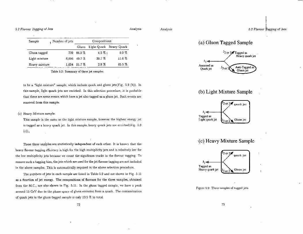
5.2 Flavour Tagging of Jets Analysis Analysis
Sample , Number of jets Compositions
’ Gluon Light Quark Heavy Quark
Gluon tagged 739 86.5 % 4.5 % ) 9.0 %
Light mixture 8,096 49.7 % 38.7 % 11.6 %
Heavy mixture 1,654 51.7 % 2.8 % 45.5 %
Table 5.2: Summary of three jet samples.
to be a “light mixture” sample, which include quark and gluon jets(Fig. 5.9 (b)). In
this sample, light quark jets are enriched. In this selection procedure, it is probable
that there are some events which have a jet also tagged as a gluon jet. Such events are
removed from this sample.
(c) Heavy Mixture sample:
This sample is the same as the light mixture sample, however the highest energy jet
is tagged as a heavy quark jet. In this sample, heavy quark jets are enriched(Fig. 5.9
(cl).
These three samples are statistically independent of each other. It is known that the
heavy flavour tagging efficiency is high for the high multiplicity jets and is relatively low for
the low multiplicity jets because we count the significant tracks in the flavour tagging. To
remove such a tagging bias, the jets which are used for the jet flavour tagging are not included
in the above samples. This is automatically required in the above selection procedure.
The numbers of jets in each sample are listed in Table 5.2 and are shown in Fig. 5.11
as a function of jet energy. The compositions of flavoum for the three samples, obtained
from the M.C., are also shown in Fig. 5.11. In the gluon tagged sample, we have a peak
around 15 GeV due to the.phase space of gluon emission from a quark. The contamination
of quark jets in the gluon tagged sample is only 13.5 % in total.
s(c) Heavy Mixture Sample
Figure 5.9: Three samples of tagged jets.
72 73
5.2 Flavour If agging of Jets i :
(a) Gluon Tagged Sample
Tagged as
(b) Light Mixture Sample
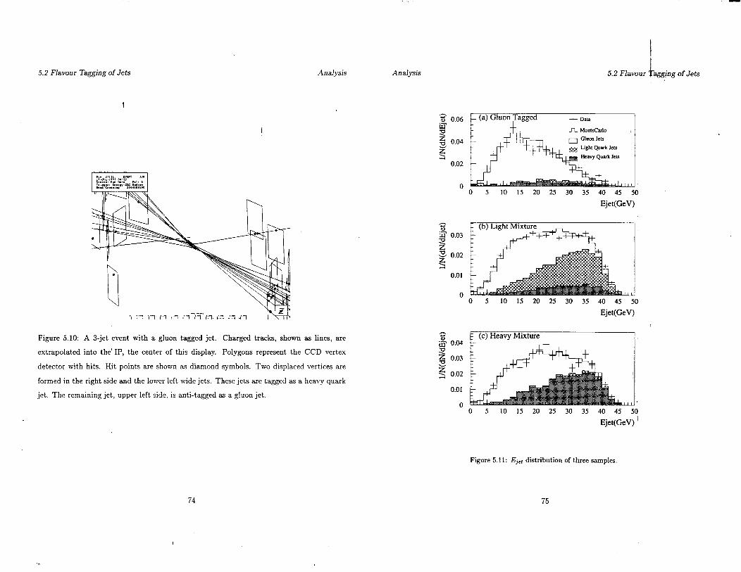
5.2 Flavour Tagging of Jets Analysis
Figure 5.10: A S-jet event with a gluon tagged jet. Charged tracks, shown as lines, are
extrapolated into the’ IP, the center of this display. Polygons represent the CCD vertex
detector with hits. Hit points are shown as diamond symbols. Two displaced vertices are
formed in the right side and the lower left wide jets. These jets are tagged as a heavy quark
jet. The remaining jet, upper left side, is anti-tagged as a gluon jet.
5.2 Flavour i aggjng of Jets I
3 0.06 .- % JL MonteCarlo
2 z 0.04
5 0.02
0 0 5 10 15 20 25 30 35 40 45 50
Ejet(GeV)
% 3 0.03 9 z
z 0.02 0.01
0 0 5 10 15 20 25 30 35 40 45 0
Ejet(GeV)
3 3 0.04
2 0.03
g 0.02
0.01
0 0 5 10 15 20 25 30 35 40 45 50
Ejet(GeV) ’
Figure 5.11: Ej,r distribution of three samples.
74 75

5.3 Comparison of Jet Properties for Raw Samples Analysis Analysis
5.3 Comparison of Jet Properties for Raw Samples I
We choose three fundamental jet properties to compare quark and gluon jets: charged mul-
tiplicity, inclusive energy fraction and jet width. In the following1 we make comparisons of
these properties between the three jet samples.
5.3.1 Charged Multiplicity
Charged multiplicity is a simple count of charged tracks assigned to a jet by the Durham
jet finder. In Fig. 5.12, the average charged multiplicities, (ncr,) , of the three samples
are shown as a function of jet energy(E+,). The error bars shown in Fig. 5.12 represent
statistical errors only. As the jet energy gets larger, the errors on the gluon tagged sample
increase, while the errors on the two other samples decrease. This is due to the statistics of
the samples as shown in Fig. 5.11. The gluon tagged and the heavy mixture have almost
the same (Q,) in all energy regions. In all energy regions, the average charged multiplicities
of the gluon tagged sample have a tendency to be larger than those of the light mixture
sample. At E,,, = 36 GeV, the charged multiplicity ratio of the gluon tagged to the light
mixture is 1.21 h 0.06, which exceeds unity by 3.5 standard deviations. Thus it is indicated
that gluon jets yield a larger multiplicity than light quarks in this energy region. (rich) of
all samples drop at last bin(E+ = 41 GeV). This can be considered that most of those jets
are from 2-jet like events and the reconstruction of jets is imperfect. Therefore, we exclude
those marginal jets from further analysis. We also exclude first bin(O < E,,, < 8 GeV) for
the same reason. In Table 5.3, the average jet energy (Ej”) , average visible energy, and
(n,,,) for three samples are listed.
5.3.2 Inclusive Energy Fraction
.
d 5.3 Comparison of Jet Properties f :r Raw Samples i
0 5 10 IS m 25 XI 35 40 45
Eu.G.V)I
Figure 5.12: Average charged multiplicities.
Inclusive energy fraction XE is defined as
(5.4)
76 77

5.3 Comparison of Jet Properties for Raw Samples
Figure 5.13: Inclusive energy fraction.
Analysis
where Ep.rtide is the energy of charged particle assumed as a pion and E,“f is the visible
energy of a jet to which the charged particle is assigned. In Fig. 5.13. the average inclusive
energy fractions, (Xn) , are shown as a function of jet energy. In this plot, the particles
between the axes of two lower energy jets are removed. This is due to an overlap of the jets
and an ambiguity of track assignment to the jet. In Fig. 5.13, the gluon tagged sample has
a softer energy fraction compared to the light mixture. This is consistent with the results
of (ncr,) , since we compare (Xn) at the same jet energy. In Table 5.3, (Xn) for the three
samples are listed.
5.3.3 Jet Width
In this analysis, the jet width is defined as the average angle, 0, between the particle mornen-
turn vector and the jet axis. In Fig. 5.14, the average jet width, (0) , is shown as a function
78
An alysk 5.4 Unfolding Distributions r Pure States i
Figure 5.14: Average jet width.
of jet energy, indicating the jet width decreases with the jet energy. The distributions for
the light mixture and the heavy mixture are the same within statistical errors However, the
gluon tagged sample has larger (0) in all energy regions except in the last bin. We exclude
tracks between two lower energy jets for the same reason as the inclusive energy fraction. In
Table 5.3, (8) for the three samples is listed.
5.4 Unfolding Distributions for Pure States
The measured distributions, shown in the previous section, are the results of mixed samples
of light quark, heavy quark and gluon states with three different fractions.’ Furthermore,
they are affected by the finite detector resolution, acceptance, and efficiency. To obtain
the distributions for pure states of light quark, heavy quark and gluon jets, we unfold the
distributions presented in the previous section, and correct for the detector effects.
79
.

-
5.4 Unfolding Distributions for Pure States
I
Analysis Analysis
Bin Sample (Ejct) ( Evis) (%h) (XE) (8)
1 Gluon Tagged 6.02 f 0.19 7.36 f 0.26 5.32 f 0.21 0.187 f 0.009 23.87 f 0.86
Light Mixture 5.59f 0.09 7.74f0.14 5.12f 0.10 0.195ztO.004 22.21 f0.35
Heavy Mixture 5.52 f 0.22 8.24 f 0.51 5.09 f 0.18 0.194 It 0.008 23.23 f 0.85
2 Gluon Tagged 12.34 f 0.14 8.73 f 0.17 5.71 f 0.15 0.175 f 0.004 23.25 f 0.46
Light Mixture 12.29 f 0.06 9.41 f 0.09 5.84 rt 0.06 0.171 f 0.002 21.79 f 0.18
Heavy Mixture 12.20 f 0.13 9.03 f 0.18 5.79 f 0.13 0.173 f 0.004 22.63 f 0.42
3 Gluon Tagged 19.95f0.17 11.55f0.27 6.79f0.19 0.147f0.004 20.20f0.44
Light Mixture 19.98f 0.05 12.63f0.10 6.47f 0.06 0.154f0.001 19.74 f0.15
Heavy Mixture 20.26 rfr 0.11 12.68 f 0.20 6.78 rt 0.12 0.147 f 0.003 19.61 f 0.31
! 5.4 Unfolding Distributions! for’Pure States
The relation between the measured and the pure states may be written
where Mgluontag.(ei), M/ightmi..(ei), and Mheovymi+. (ei) represent the measured quantities for
a given jet energy bin e;. G(ei), L(ei) and H( e, -) are the values for the pure states of gluon,
light quark and heavy quark jets, respectively. Ui, “unfolding matrix”, is the 3 x 3 matrix
for bin i, and contains all information on flavour compositions and detector effects for the
three measured samples. Therefore, Vi can be written in terms of a “composition matrix”,
C,, and a “detector effect matrix”, Di,
Ui=Ci’Di. (5.6)
The composition matrix is explicitly written
5 Gluon Taggeq 35.23 f 0.31 18.25 f 0.89 8.46f 0.42 0.118 f 0.005 18.52 f 0.70
Light Mixture 35.74 +z 0.05 19.40 z!z 0.18 6.99 + 0.06 0.142 zt 0.001 16.73 f 0.15
Heavy Mixture 35.71 f 0.12 18.75 f 0.37 7.95 & 0.17 0.124 f 0.003 16.91 f 0.31
6 Gluon Tagged 41.58 f 0.44 16.19 f 2.30 6.93 f 0.84 0.108 f 0.013 10.64 f 1.03
Light Mixture 41.73 f 0.07 20.66 f 0.45 7.14 f 0.16 0.139 & 0.003 16.31 f 0.32
Heavy Mixture 41.75 f 0.17 16.56 f 0.78 7.12 f 0.34 0.140 f- 0.007 16.78 f 0.64
4 Giuon Tagged 27.41 310.18 14.97 f 0.44 7.27 f 0.22 0.131 & 0.004 19.83 f 0.51
Light Mixture 27.98f 0.05 15.90f0.13 6.82f0.06 0.146zt00.001 18.59f 0.15
Heavy Mixture 27.78 -f 0.11 15.81 & 0.27 7.31 f 0.15 0.136 f 0.003 18.72 f 0.31
c, =
Table 5.3: Jet properties of three samples.
~IUon tag. gluon
cphon tag. ltghtpuork &$$rk
light mir. Cgluon
light miz. Clightpuark
light miz. Cheavypuork
heavymtz. Cgluon
heovymiz. ‘light quark
heovymtz. Chcovygu.rk I1 ,’ (5.7)
where ci&, ‘“Ontag. is the fraction of true gluon jets in the gluon tagged sample, and so on. The
detector effect matrix is a diagonal matrix
. (5.8)
I The pure states of gluon, light quark, and heavy quark can be obtained by inverting
eq. 5.5 I
80
.
81
5.4 Unfolding Distributions for Pure States
M gh0n h,.(G)
&ghtmi+. (ei)
M heavymiz. (ei)
Analysis
To obtain the composition matrices and the detector effect matrices, two sets of hl.C.
are used: the hadron level Monte Carlo and the detector level Monte Carlo:
1. Hadron level Monte Carlo
200,000 events are generated by the JETSET 6.3 without any detector simulation.
Only charged particles with generated momenta are used for the analysis. Jets are
determined by the Durham jet finder with ycut value 0.007, as the same value as used
in the data analysis. Their flavour are tagged using generator information.
2. Detector level Monte Carlo
This is the M.C. described in chapter 3.3. About 360,000 events are generated by the
JETSET 6.3, and are processed by the SLD simulation program. The output data of
M.C., which is the same format as the data, is analyzed by exactly the same procedure
as the real data.
The composition matrices are determined by the detector level M.C. which has in-
formation on generated jet flavour and flavour tagged by the analysis. The composition
matrices for each jet energy bin are listed in Table 5.4. From the table, the gluon jet fraction
in the gluon tagged sample amounts to a high value of 93.5% at the jet energy 8 - 16 GeV.
However, the gluon jet fraction in both the light and the heavy mixtures are also high. This
is the reason why we do not expect to observe significant differences in the distributions
presented in previous section. At high energy(32 - 40 GeV) region, the gluon, light, and
heavy quark fractions are dominant in the gluon tagged, light, and heavy mixture samples,
respectively. We observe differences among the three samples at the high energy.
The diagonal elements of the detector effect matrices are obtained by the bin-by-bin
In Fig. 5.15(a), the unfolded (r&h) and their statistical errors for gluon, light quark and
heavy quark jets are shown as a function of jet energy. While the statistical errors in the
lower energy bins are larger than the differences between gluon and quark jets, it is obvious
that gluon jets have the largest value in all energies and light quark jets have the smallest
value in most energy regions except the lowest energy bin.
A function (rich) = ~ln(Ej,~) + b is used to fit those distributions., The fitted curves
are also shown in Fig. 5.15 for these distributions. Fitted values of a, b and reduced x2 are
listed in Table 5.5. (r&h) of heavy quark jets is well described by the function with reduced
x2 0.2. Except for the last bin, gluon jets also well described by the function. The fitted
function of light quark jets is almost flat due to a drop of the last bin which has a small
error.
82 83
. Analysis 5.5 Comparison for Pure,State Samples
I correction method using the above two sets of M.C.
G(ei) d,, = ~ M&,,(ei) ’
42 = L(G)
M;ightpuark (ei) ’
43 =. H(ei)
MLvy puotk (4 ’ ,
where M&n(ei)j M&htpuork(ei) and MLeovypuark(ei) are calculated by
(5.10)
(5.11)
In Table 5.4, the diagonal elements of the correction matrix are listed. At the high energy,
the correction factors deviate from unity largely.
5.5 Comparison for Pure State Samples
5.5.1 Average Charged Multiplicity

5.5 Comparison for Pure State Samples Analysis Analysis
I 5.5 Comparison for Pur d State Samples
Jet energy bin(GeV) , Composition matrices Correction matrices
bch) WE) ’ (0)
plum tog. gl”.” log. ghon
i ,
Clighl quark pm Log. /kl\ /
he.vyquork
i
11 41 41
lighlmir Cglvon
,igh!ml.. %ghtpvorC
lrghtmir. %e.vyquorC \’ 42 42 62
hewy mlt. Cgluon
he.yJ mi.. %ghtp.rC
heavy mir. Chewyquork 43 J \ 43 / \ 43
0.935 0.017 0.048 \ f 0.98 \ / 1.02 ’ ( 0.90
8- 16 0.776 0.180 0.044 1.18 0.75 0.91
\ 0.792 0.018 0.190 , \ 1.20 J \ 0.80 ) \ 0.89
1 0.880 0.034 0.086 \ ( 1.00 1 ( 1.03 \ / 0.93
16-24 0.609 0.297 0.094 1.02 0.97 0.92
\ 0.648 0.020 0.332 , \ 0.98 J \ 0.94 / i 0.83
’ 0.805 0.090 0.105 ’ / 1.00 1 / 1.06 \ / 0.98
24 N 32 0.406 0.451 0.143 0.95 0.93 O.i6
\ 0.416 0.030 0.554 J \ 1.06 ) \ 0.90 / \ 0.85
/ 0.659 0.148 0.193 1 / 0.88 \ ( 1.22 \ ( 1.06
32 N 40 0.220 0.608 0.172 1.05 0.71 0.63
\ 0.238 0.043 0.719 / \ 1.10 ) \ 0.89 ) \ 0.89
Table 5.4: Summary of the composition and the correction matrices. Only the diagonal
elements are listed for the correction matrices. The off-diagonal elements of the correction
matrices are zero.
Jet flavour a b reduced x2
Gluon jet 2.6 zt 0.5 -0.7 f 1.3 2.7
LYght quark jet 0.2 3~ 0.6 5.1 f 2.1 0.7
Heavy quark jet 1.5 i 0.9 1.7f3.0 0.2 Figure 5.15: Average charged multiplicities (rich) and their ratios.
Table 5.5: Fitted values and reduced x’.
84 85
- Gluon Jets - - - - - Light Quark Jets
...--....- Heavy Quark Jets
P 2
2 1.6 E a 2 1.6
sj 1.4 a g 1.2
2 1
0.6
0.6
0.4
0.2
0
(b)
SLD
6
5 0.6
Jet Energy (Gev)
Jet Energy (GeV) 1 Jet Energy (GeV)
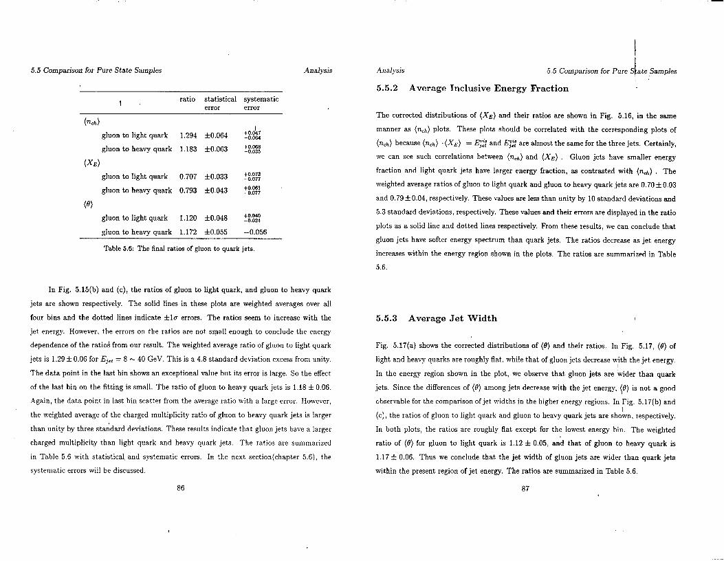
5.5 Comparison for Pure State Samples Analysis
I ratio statistical systematic
error error
bbh) I
gluon to light quark 1.294 f0.064 :;:g
gluon to heavy quark 1.183 f0.063 ‘;:E
(XE)
gluon to light quark 0.707 f0.033 ?I;::
gluon to heavy quark 0.793 f0.043 +o.om -0.077
(*)
gluon to light quark 1.120 f0.048 ‘g$j
gluon to heavy quark 1.172 f0.055 -0.056
Table 5.6: The final ratios of gluon to quark jets.
In Fig. 5.15(b) and (c), the ratios of gluon to light quark, and gluon to heavy quark
jets are shown respectively. The solid lines in these plots are weighted averages over all
four bins and the dotted lines indicate flu errors. The ratios seem to increase with the
jet energy. However, the errors on the ratios are not small enough to conclude the energy
dependence of the ratios from our result. The weighted average ratio of gluon to light quark
jets is 1.29 f 0.06 for Ej,t = 8 - 40 GeV. This is a 4.8 standard deviation excess from unity.
The data point in the last bin shows an exceptional value but its error is large. So the effect
of the last bin on the fitting is small. The ratio of gluon to heavy quark jets is 1.18 rt 0.06.
Again, the data point in last bin scatter from the average ratio with a large error. However,
the weighted average of the charged multiplicity ratio of gluon to heavy quark jets is larger
than unity by three standard deviations. These results indicate that gluon jets have a larger
charged multiplicity than light quark and heavy quark jets. The ratios are summarized
in Table 5.6 with statistical, and systematic errors. In the next section(chapter 5.6), the
systematic errors will be discussed.
86 87
Analysis 1 5.5 Comparison for Pure S, ate Samples I
5.5.2 Average Inclusive Energy F’raction
The corrected distributions of (Xs) and their ratios are shown in Fig. 5.16, in the same
manner as (r&h) plots. These plots should be correlated with the corresponding plots of
(n,h) because (n,,+) ‘(Xa) = E$ and E$ are almost the same for the three jets. Certainly,
we can see such correlations between (n&) and (Xn) Gluon jets have smaller energy
fraction and light quark jets have larger energy fraction, as contrasted with (nd) . The
weighted average ratios of gluon to light quark and gluon to heavy quark jets are 0.70 f 0.03
and 0.79 f 0.04, respectively. These values are less than unity by 10 standard deviations and
5.3 standard deviations, respectively. These values and their errors are displayed in the ratio
plots as a solid line and dotted lines respectively. From these results, we can conclude that
gluon jets have softer energy spectrum than quark jets. The ratios decrease as jet energy
increases within the energy region shown in the plots. The ratios are summarized in Table
5.6.
5.5.3 Average Jet Width
Fig. 5.17(a) shows the corrected distributions of (0) and their ratios. In Fig. 5.17, (13) of
light and heavy quarks are roughly flat, while that of gluon jets decrease w!th the jet energy.
In the energy region shown in the plot, we observe that gluon jets are hider than quark
jets. Since the differences of (0) among jets decrease with the jet energy, (0) is not a good
observable for the comparison ofjet widths in the higher energy regions. In Pig. 5.17(b) and
(c), the ratios of gluon to light quark and gluon to heavy quark jets are shown, respectively.
In both plots, the ratios are roughly flat except for the lowest energy bin. The weighted
ratio of (0) for gluon to light quark is 1.12 f 0.05, and that of gluon to heavy quark is
I.17 * 0.06. Thus we conclude that the jet width of gluon jets are wider than quark jets
within the present region of jet energy. The ratios are summarized in Table 5.6.

5.5 Comparison for Pure State Samples Analysis Analysis
- Gluon Jets ----- Light Quark Jets .......... Heavy Quark Jets
F 2
I 1.8 E a 2 1.6
2 1.4 0 g 1.2
2 1
0.6
0.6
0.4
0.2
0
2
1.6
1.6
1.4
1.2
0.6
0.6
0.4
0.2
0
1 (b)
Jet Energy (GeV)
I I
I
SLD I / / I I I I I I, I I / 1,
10 20 30 40
Jet Energy (GeV)
30 40
Jet Energy (GeV)
Figure 5.16: Average inclusive energy fractions (XE) and their ratios.
88 89
25 -
++ -___ I. -_-. I I -mu nrn,
. . . . . . . . . . . . it- ____ _-. . . . . . . : . . . . . ...! . . . . .
- Gluon Jets ----- Light Quark Jel .......... Heavy Quark JI
Jet Energy (GeV)
* i 5.5 Comparison for Pur State Samples i
0 ‘IIII’lI(I’I’/II 10 20 30 40
Jel Energy (GeV)
2 L
1.8 :
1.6 :
1.4 :
1.2 -’ _’ ! I L I .:. I--
1 I
0.8 :
0.6 ;
0.4 :
0.2 F(c) SLD 0 F’ I ’ I ” ” I ’ I I / ’ 1
10 20 30 40
’ Jet Energy (GeV)
Figure 5.17: Average jet widths (0) and their ratios.
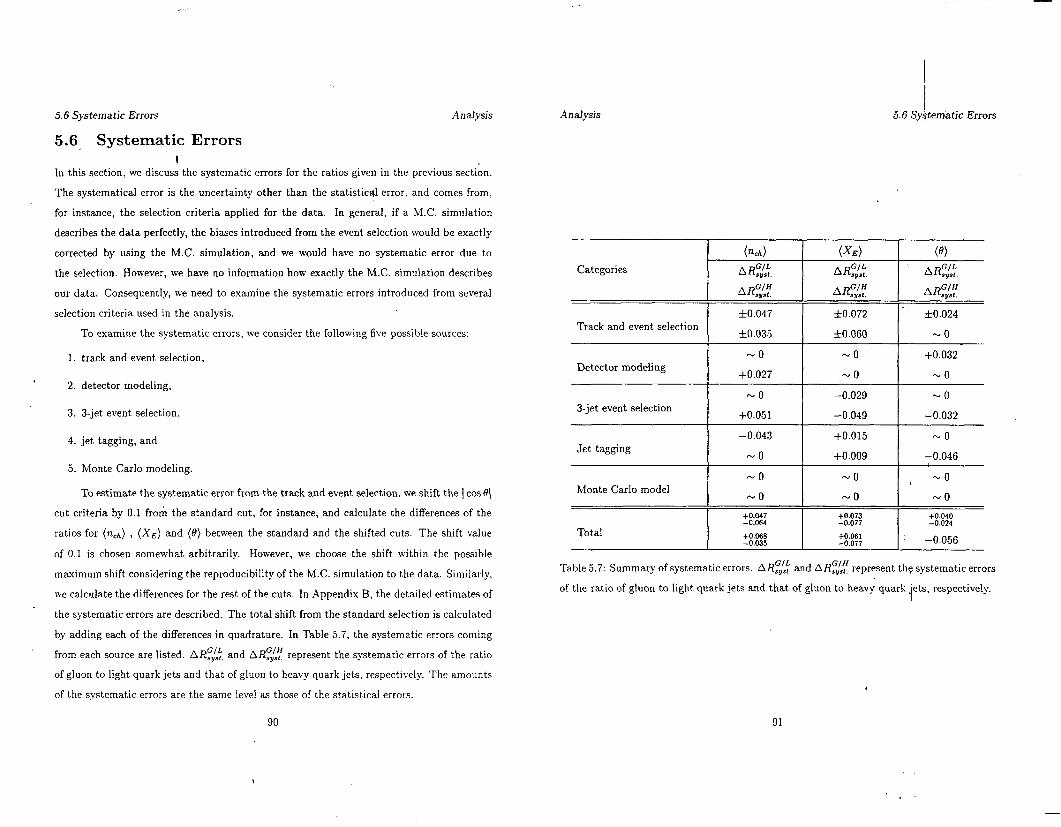
5.6 Systematic Errors AnaJysis I
5.6 Sy.$ten&ic Errors
5.6, Systematic Errors 1
In this section, we discuss the systematic errors for the ratios given in the previous section.
The systematical error is the uncertainty other than the statisticrjl error. and comes from,
for instance, the selection criteria applied for the data. In general, if a M.C. simulation
describes the data perfectly, the biases introduced from the event selection would be exactly
corrected by using the M.C. simulation, and we would have no systematic error due to
the selection. However, we have no information how exactly the M.C. simulation describes
our data. Consequently, we need to examine the systematic errors introduced from several
selection criteria used in the analysis.
To examine the systematic errors, we consider the following live possible sources:
1. track and event selection,
2. detector modeling,
3. 3-jet event selection,
4. jet tagging, and
5. Monte Carlo modeling.
To estimate the systematic error from the track and event selection, we shift the 1 cos f?(
cut criteria by 0.1 from the standard cut, for instance, and calculate the differences of the
ratios for (rich) , (Xs) and (8) between the standard and the shifted cuts. The shift value
of 0.1 is chosen somewhat arbitrarily. However, we choose the shift within the possible
maximum shift considering the reproducibility of the M.C. simulation to the data. Similarly,
we calculate the differences for the rest of the cuts. In Appendix B, the detailed estimates of
the systematic errors are described. The total shift from the standard selection is calculated
by adding each of the differences in quadrature. In Table 5.7, the systematic errors coming
from each source are listed. ARf$, and ARfisf represent the systematic errors of the ratio
of gluon to light quark jets and that of gluon to heavy quark jets, respectively. The amounts
of the systematic errors are the same level as those of the statistical errors.
Track and event selection
Detector modeling -0
+0.027
J-jet event selection
Jet tagging -0.043
-0
Monte Carlo model -0
-0
Total
rtO.072 ’ ztO.024
fO.060 -0
-0 +0.032
-0 -0
-0.029 -0
-0.049 -0.032
+0.015 -0
f0.009 -0.046
Table 5.7: Summary of systematic errors. ARS’,l,:: and AR:<: represent the systematic errors
of the ratio of gluon to light quark jets and that of gluon to heavy quark ‘ets, respectively. i
90 91
5.6 Systematic Errors Analysis
Chapter 6
Summary
In this thesis, we have studied quark and gluon jet differences in 3-jet events of .Z”
hadronic decays with charged tracks. The use of weighted impact parameters allows us
to identify the flavour of jets, as light or heavy quark jets. Gluon jets are collected by
anti-tagging of heavy quark jets with a purity of 86.6% estimated from the Monte Carlo
simulation. For comparison, we considered the light mixture and the heavy mixture of
quark and gluon jets. The light and the heavy mixture samples consist of two lower energy
jets of 3-jet events in which the highest jet is tagged as a light quark jet or a heavy quark
jet, respectively. These three samples are statistically independent. The jets used for jet
flavour tagging are not included in the three samples so that the bias introduced by the jet
flavour tagging was minimized.
Three observables are chosen to compare the jet properties:thk charged multiplicity
(R~,,) , the inclusive energy fraction of particles (Xa) , and the average angle between the
particle momentum and the jet axis (0) , called the jet width. By t,he use of the M.C.
simulation, the distributions of jet properties obtained from the three samples are unfolded
to obtain the properties for pure states of gluon, light quark, and heavy quark jets. The
observables for pure states include corrections for the detector resolution and acceptance.
Our results show that (R~,,) of gluon jets are larger than those of light quark and heavy
quark jets in the jet energy region of 8 GeV to 40 GeV. The Iatios of (rich) increases with
93 92
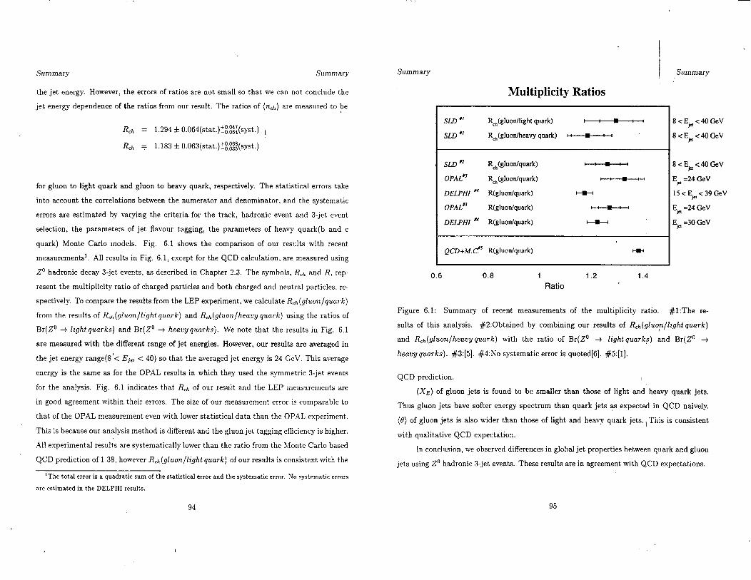
Summary Summary
the jet energy. However, the errors of ratios are not small so that we can not conclude the
jet energy dependence of the ratios from our result. The ratios of (n,~,) are measured to be
Rch = 1.294 f O.O64(stat.)?i:$:(syst.) t
R ch f 1.183 f O.O63(stat.)?~$~(syst.)
for gluon to light quark and gluon to heavy quark, respectively. The statistical errors take
into account the correlations between the numerator and denominator, and the systematic
errors are estimated by varying the criteria for the track, hadronic event and 3-jet event
selection, the parameters of jet flavour tagging, the parameters of heavy quark(b and c
quark) Monte Carlo models. Fig. 6.1 shows the comparison of our results with recent
measurements’. All results in Fig. 6.1, except for the QCD calculation, are measured using
Z” hadronic decay 3-jet events, as described in Chapter 2.3. The symbols, R,h and R, rep-
resent the multiplicity ratio of charged particles and both charged and neutral particles, re-
spectively. To compare the results from the LEP experiment, we calculate R,h(gluon/quark)
from the results of &h(gluOn/light quark) and &(ghOn/heuvy quark) using the ratios of
Br(Z” + Eight quarks) and Br(Z” + heavy quarks). Vde note that the results in Fig. 6.1
are measured with the different range of jet energies. However, our results are averaged in
the jet energy range(8 ‘< Ej,t < 40) so that the averaged jet energy is 24 GeV. This average
energy is the same as for the OPAL results in which they used the symmetric 3-jet events
for the analysis. Fig. 6.1 indicates that R,h of our result and the LEP measurements are
in good agreement within their errors. The size of our measurement error is comparable to
that of the OPAL measurement even with lower statistical data than the OPAL experiment.
This is because our analysis method is different and the gluon jet tagging efficiency is higher.
.411 experimental results are systematically lower than the ratio from the Monte Carlo based
QCD prediction of 1.38, however &(gluon/light quark) of our results is consistent with the
‘The total error is a quadratic sum of the statistical error and the systematic error. IVo systematic errors
are estimated in the DELPHI results.
Summary
0.
-
Multiplicity Ratios
SLD rtl Rc,(gluon/light quark) ,: 3 :I 8<Ejcl<40GeV
SW #’ Rc,(gluotieavy quark) m 8<Ejne40GeV
SW” R,(gluon/quark) 0: q :a
OPA Ls3 R&luon/quark) 8: y :4
DELPHI M R(gluonlquark) l-m-4
OPAL”.’ R(gluon/quark) P: =:,
DELPHI M R(gluon/quark) M
8<Einc40GeV
E,, =24 GeV
15<Ejnc39GeV
EM =24 GeV
Ej,, =30 GeV
QCD+M.C? Wgluodquark)
6 0.8 1 1.2 1.4
Ratio
Summary
Figure 6.1: Summary of recent measurements of the multiplicity ratio. #l:The re-
sults of this analysis. #2:0btained .by combining our results of &(glUO?/light quark)
and R,h(g[zlon/heavyquarl;) with the ratio of Br(Z’ + lightquarlip) and Br(Z” +
heavy quarks). #3:[5]. #4:No systematic error is quoted[6]. #5:[1].
QCD prediction.
(X,) of gluon jets is found to be smaller than those of light and heavy quark jets.
Thus gluon jets have softer energy spectrum than quark jets +s expected in QCD naively.
(0) of gluon jets is also wider than those of light and heavy quark jets., This is consistent
with qualitative QCD expectation.
In conclusion, we observed differences in global jet properties between quark and gluon
jets using Z” hadronic 3-jet events. These results are in agreement with QCD expectations.
94 95

Summary Summary
Bibliography
96
[I] I. M. Dremin and R. C. Hwa, Average multiplicities in gluon and quark jets as exact
solution of QCD equations, Phys. Lett. B 324(1994)477-481
[2] JADE Collaboration, W. Bartel et. al., Experimental evidence for differences in (pl)
between quark jets and gluon jets, Phys. Lett. 123B(1983)460;
UA2 Collaboration, P. Bagnaia et. al., Measurement of jet fragmentation properties at
the CERN pp collider, Phys. Lett. 144B(1984)291;
Mark II Collaboration, A. Peterson et. al., Inclusive charged-particle distribution in
nearly threefold-symmetric three-jet events at E,,, = 29 GeV, Phys. Rev. Lett.
55(1985)1954;
UAl Collaboration, G. Arnison et. al., Analysis of the fragmentation properties of quark
and gluon jets at the, CERN SPS pp collider, Nucl. Phys. B276( 198’6)253;
TASS0 Collaboration, W. Braunschweig et al., Z. Phys. C45(1989)1;
AMY Collaboration, Y. K. Kim et al., Comparison of quark and g]uon jets produced in
high-energy e+e- annihilations, Phys. Rev. Lett. 63(1989)1772;
[3j HRS Collaboration, M. Derrick et. al., Phys. Lett. B 165( 1985)449:
[4] OPAL Collaboration, G. Alexander et. al., A direct observation of quark-gluon jet
differences at LEP, Phys. Lett. B265(1991)462; I
[5] OPAL Collaboration, P. D. Acton et. al., A study of differences between quark and gluon
jets using vertex tagging of quark jets, CERN-PPE/93-02, Z. Phys. C58(1993)387.
97
BIBLIOGRAPHY BIBLIOGRAPHY BIBLIOGRAPHY El BI LIOGRAPHY
PI Stefan UberschLr(DELPH1 collaboration), talk presented at the 8th DPF Meeting, Al- Phys. B178(1981)421; K. Fabricius, G. Kramer, G. Schierholz and I. Schmitt, Z. Phys.
buquerque, New Meyico, 1994. C11(1982)315; F. Gutbrod, G. Kramer and G. Schierholz, Z. Phys. C21(1984)235.
I71 E. D. Commins and P. H. Bucksbaum, Weak interactios of leptons and quarks; G. Kane, WI Modern elementary particle physics,;
PI
PI
Particle Data Group, L. Montanet et al., Phys. Rev. D 50(1994).
Richard D. Field, Applications of perturbative &CD, Redwood City, USA: Addison-
Wesley(1989).
PI
P31
PO1
1111
P-4
Donald H. Perkins, Introduction to high energy physics, Third Edition.
G. Preparata, Why are quarks(and gluons) confined?, MITH93/18.
CDF Collaboration, F. Abe et. al., Evidence for top quark production in pp collisions
at fi = 1.8 TeV, FERMILAB-PUB-94/097-E, Phys. Rev. D50(1994)2966.
J. B. Gaffney and A. H. Mueller, Nucl. Phys. B 250(1985)109.
G. Marchesini et al., Comp. Phys. Comm. 67(1992)465.
Yoshihito Iwasaki(SLD collaboration), talk presented at the 8th DPF Meeting, Albu-
querque, New Meyico, 1994, SLAC-PUB-6597, TOHOKU-HEP-94-02.
Thomas D. Gottschalk, Hadronizatin and fragmentation, CALT-68-1075.
P. Mattig, The structure of jets in e+e- collisions, Physics Reports(Review section of
Physics Letters) 177, Nos 3&4(1989)141-317.
G. Altarelli and G. Parisi, Nucl. Phys. B 126(1977)298.
J. Ellis, M. K. Gaillard and G. G. Ross, Nucl. Phys. B111(1976)253.
A. Ali, J.G. Korner, Z. Kunszt, E. Pietarinen, G. Kramer, G. Schierholz and J. Will-
rodt, Nucl. Phys. B167(1980); R. K. Ellis, D. A. Ross and E. A. Terrano, Nucl.
P41
1251
WI
P31
(141
1151
1271
P-4
1161
1171
PI
1301
P31
PI
PO1
1311
1321
98
I ,’
Torbjijrn Sjiistrand, The LUND Mote Carlo for jet fragmentation and e+e- physics -
JETSET version 6.2, Comput. Phys. Commun. 39(1986)347-407.
R. D. Field and S. Wolfram, Nucl. Phys. B 213(1983)65.
L. Lonnblad, Comput. Phys. Commun. 71(1992) 15; U. Pettersson,‘ARIADNE, A Monte
Carlo for QCD cascades in the colour dipole formulation’, LU TP 88-5(1988).
G. Gustafson, Phys. Lett. B 175(1986) 453
T. SjGstrand, QCD generators, Z Physics at LEP I, CERN 89-08, Volume 3 (1989)
G. Blaylock. The WISRD beam energy measurement. SLD Physics Note 22, SLAC(June
1993); J. Kent et al. SLAC-PUB-4922(March 1989).
SLD Collaboration. First measurement of the left-right cross section asymmetry in Z
boson production by e+e- collisions. Phys.Rev.Lett, 70(17):2515(1993)
SLD Collaboration. Precise measurement of the left-right cross-section asymmetry in Z
boson production by e+e- collisions. Phys.Rev.Lett, 73(17):25-29(1994)
SLD Design Report, SLAC-Report-273(1984)
M.G. Strauss et al., in the proceedings fo the 7th Meeting of the’American Physical
Society, Division of Particles and Fields, p. 1758. G. Charpak and F. Sauli, Annu. Rev.
Nucl. Part. Sci. 34:285(1984).
Jan A. Lauber, A study of jet rates and measurement of cx, at the Z” resonance. Ph.D
thesis.
GEANT 3.15 program, CERN Application Software Group, CERN Program Li-
brary( 1993).
99
BIBLIOGRAPHY
. I BIBLIOGRAPHY BIBLIOGRAPHY b Bl, LIoGRAPHY
I
TASS0 Collaboration, W. Braunschweig et. atl., Z. Phys. C41 359(1988); P. N. Burrows, [46] H.Park, R. Ben David, R. Dubois, R. Frey and P.C. Rowson, Event selection for the
Z. Phys. C41, 375( 1888). 1992 ALE analysis, SLD Physics Note No. 17. (331
1341
1351
[361
[371
1381
1391
[401
1411
I421
OPAL Collaboration, M. Z. .4krawy et al., Z. Phys. C47, 5Oq(1990).
C. Peterson, D. Schlatter, I. Schmitt and P. M. Zerwas, Phys. Rev. D27 105(1983).
ALEPH Collaboration, D. Buskulic et. al., Z. Phys. C62 179(1994); L3 Collaboration,
B. Adeva et. al., Phys. Lett. B261 177(1992); OPAL Collaboration, R. Akers et. al., Z.
Phys. C61 209(1994); DELPHI Collaboration, P. Abreu et. al., Z. Phys. C59 533(1993).
OPAL Collaboration, P. D. Acton et. al., Z. Phys. C53 539(1992).
SLD Collaboration, K. Abe et. al, Measurement of Rb with impact parameters and
displaced vertices, SLAC-PUB 6569.
N. Isgur, D. Scora, B. Grinstein and M. B. Wise, Phys. Rev. D39 799(1989) PUB-6292(1993)
M. Artuso(CLE0 Collaboration), HEPSY-7-93, talk presented at Workshop on b [52] SLD Collaboration, K. Abe et al., Measurement of the charged multiplicity of Z” + b6
Physics at Hadron Accelerators( 1993). events, Phys. Rev. Lett., 72(20):3145-3149(1994).
CLEO Collaboration, G. Crawford et. al., Phys. Rev. D45 725(1992).
F. Muheim(CLE0 Collaboration), talk presented at the 8th DPF Meeting, Albu-
querque, New Mexico, 1994.
[43] ARGUS Collaboration, H. Albrecht et. at., Z. Phys. C58 191(1993); ARGUS Collabo-
ration, H. Albrecht et. at., Z. Phys. C62 371(1994).
[44] David C. Williams, The left-right forward-backward asymmetry for b quarks at the
SLD. Ph.D thesis.
[45] John M. Yamartino, Hadronic event selection using the LAC, SLD Physics Note No.
14.
100
[47] Vernon D. Barger and Roger J. N. Phillips, Collider Physics, Redwood City, USA:
AddisonWesley(l987).
[48] Jan A. Lauber, Ph.D Thesis, SLAC-Report-413(1993). ,
[49] R. Ben-David, H. Park, Background Measurement for the 1992 ALR Analysis, SLD
Physics Note No. 18.
[50] S. Cantani et al., Phys. Lett. B 269(1991) 432; N. B rown and W. J. Stirling, Z. Phys.
C 53(1992) 629; S. Bethke, Z. Kunszt, D. Soper and W. J. Stirling, Nucl. Phys. B
370(1992) 320.
[51] SLD Collaboration, K. Abe et al., A Measurement of Rb = ,.c,&(~~$@sJ at SIB, SLAC-
101
BIBLIOGRAPHY BIBLIOGRAPHY
102
I
Appendix A
SLD Collaboration
. Adelphi University
Robert Steiner
l INFN Sezione di Bologna
l Brunei University
Adrian McKemey, Steve Watts, Nicholas Allen, Erez Etzion
l Boston University
John Coller, James Shank, J. Scott Whitaker, Sarah Hedges
. University of Cincinnati
Brian Meadows, Mirko Nussbaum
. California Institute of Technology
. University of Colorado
Gregory Baranko, Nety Krishna, Uriel Nauenberg, Kathy Oliver, Cheng-Gang Fan
l Columbia University
Michael Shaevitz, Srinka Ghosh, John Son, Peter Rowson
103
SLD Collaboration
. Colorado State University
Bob Wilson, Mihdi Dima
. INFN Sezione di Ferrara
Barbara Camanzi, Edoardo Mazzucato, Livio Piemontese
. Lab. Nazionali di Frascati
Alessandro Calcaterra, Riccardo Desangro, Ida Peruzzi, Marcello Piccolo
SLD Collaboration SLD Collaboration Collaboration
l Nagoya University
Ryoichi Kajikawa, Akira Sugiyama, Shiro Suzuki, Yukiyoshi Ohnishi, Kenji Abe
. University of Illinois
Bob Eisenstein, Gary Gladding, Inga Karliner, Andrew Foland
. Northeastern University
. University of Oregon
Jim Brau, Raymond Frey, Jingchen Zhou, Jennifer Huber, Matthew Langston, Xiaox-
ing Yang, Nikolai Sinev, Hyun Hwang
. Universita di Padova
. Universita di Perugia, Sezione INFN
Giampiero Mancinelli, Giancarlo vantovani, Donatella Falciai, Roberto Massetti . KEK National Lab
. INFN, Sezione di Pisa . Lawrence Berkeley Laboratory
Bruce Schumm, Gil Shapiro, Herbert Steiner
. Louisiana Technical University
Kathleen Johnston, Basem Barakat, Jeff Smith, Eric Burch
. University of Massachusetts
Stanley Hertzbach, Richard Kofler, Michael Strauss, Aurel Trandafir
. University of Mississippi
Robert Kroeger, Jim Reidy
. Massachusetts Institute of Technology
Philip Burrows, Sandra Fowler, Henry Kendall, Louis Osborne, Dale Ross. Frank Tay-
lor, Robin Verdier, Ray Cowan, Michael Fero, Jim Quigley, Eric Torrence, Richard
Yamamoto, Zhibo Zhang
104
l Rutherford Appleton Laboratory
Chris Damerell, Tony Gillman, Fred Wickens, David Jackson
l Rutgers University
Kenneth Baird, Pieter Jacques, Mohan Kalelkar, Richard Plano, Peter Stamer
. Stanford Linear Accelerator Center
Daniel Alzofon, Jack Hoeflich, Bill Wisniewski, X&fan Zhou, David Galloway, Em-
lyn Hughes, Ross King, Thomas Markiewicz, Takashi Maruyama, Hiroaki Masuda,
Kenneth Moffeit, Charles Prescott, Leon Rochester, Owen Sax on, \
Morris Swartz,
Tracy Usher, Charles Young, Mike Woods, Mourad Daoudi, Andrea Davies, David As-
ton, Hideaki Kawahara, David Leith, Matt McCulloch, Don McShurlei, David Muller,
Gerard Oxoby, Tom Pavel, Blair Ratcliff, Robert Reif, Constantine Simopoulos, Paul
Stiles, Jaroslav Vavra, Tom Weber, Malcolm Lewis, Lilian DePorcel, Paul Rensing,
Thomas Mattison, Alexei Tolstykh, Colin Jessop, Stephen Schaffner, Mary King, John
105

SLD Collaboration SLD Collaboration
Jaros, Dong Su, Tom Junk, Rafe Schindler, Homer Neal, Bill Burgess, Wesley Crad-
dock, Vickee Flynn,IDavid Burke, Michael Hildreth, Greg Punkar, Steve Wagner,
Timothy Barklow, Richard Boyce, Stephen Williams, Barbara Barrera, Joanne Bog-
art, Gary Bower, Martin Breidenbach, Ronald Cassell, Bernie k ulver, Richard Dubois,
Justin Escalera, Dietrich Freytag, Mark Freytag, Gunther Hailer, Vern Hamilton,
Karen Heidenreich, John Hodgson, Mike Huffer, Harvey Lynch, Robert Messner, Len
Moss, Kazuko Onaga, Joseph Perl, Gerard Putallaz, James Russell, Philip Seward,
Stephen Smith, Anthony Waite, Ramon Berger, Kris Dudley, Michael Foss, Jessie
Gutierrez, Gibson Locke, Raymond Rodriguez, Donald Peterson, Takashi Akagi, Skap-
pass VIII Knut, Anthony Johnson, Eric Vella, Aaron Chou, Glen Crawford, Howard
Rogers, James Davis, Gregory Rogers
0 Sogang University
Yongduk Kim, Hyejoo Kang, Dongwk Hwang
l University of Tennessee
Steve Berridge, Bill Bugg, Hans Cohn, Peter Du, Hilman Hargis, Edward Hart, Achim
Weidemann, Sharon White, Konstantine Shmakov
l Tohoku Univeisity
Koya Abe, Yoji Hasegawa, Kazumi Hasuko, Yoshihito Iwssaki, Tadashi Nagamine,
Shinya Narita, Fumihiko Suekane, Haruo Yuta
l U.C. Santa Barbara
Debbie Ceder, Adolph Lu, Steven Yellin
0 U.C. Santa Cruz
SLD Collaboration
l Vanderbilt University
Robert Panvini, Terry Reeves, John Venuti
l University of Washington
Toby Burnett, Victor Cook, Ji Ma, Paul Mockett, Anthony Szumilo, Eric Church,.Eric
Weiss .
0 University of Wisconsin
Henry Band, Jim Johnson, Richard Prepost, Geordie Zapalac, Victor Serbo
l Yale University
Charles Baltay, William Emmet, Steven Manly, Jeffrey Snyder, Stephane Willocq,
Sumit Sen, Jinchun Kou, Ming Liu
Guy Blaylock, Don Coyne, Georgia Hamel, Xi Liu, Terry Schalk, Michael Schneider,
David A. Williams, James Mattingly
106 107

SLD Collaboration SLD Collaboration
108
Appendix B
Systematic Errors
In this appendix, we examine the experimental systematic errors of the ratios obtained in pre-
vious section. The systematic errors are the experimental biases introduced by the detector
acceptance, efficiency and resolution, and by the detector simulation, event reconstruction,
and by the several selection criteria applied to the data for this analysis, and by the bottom
and charm quarks parameters used in M.C. simulation which are used for the jet flavour
tagging, unfolding and corrections. The possible systematic error sources are divided into
five categories as follows.
1. Track and event selection
For the track and event selection category, we apply the tight cuts of the selection
criteria one by one to see the sensitivity on the cut values. Loose cuts are not applied
because the disagreements between the data and the M.C. are observed in the region
of the loose cuts, and may cause imperfect corrections of the deteqtor acceptance and
efficiency. In Table B.l, the variations of the selection criteria are listed. Each set of
variations are applied for both the data and the M.C with the same analysis procedure,
and then compared against the standard cuts
AR = Rm - Rstd,
109
P.1)
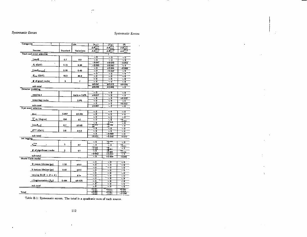
Systematic Errors Systematic Errors
Categorica I CUU (“rd I (X.5) I (8) AR.:,,. b‘ 1 AR.,/., L 1 LL
Sources AR,./.,
Standard Varialion* i,” AR.:.,. 1 AR.,/,, l,” 1 AR.,7 ca
‘Itut and event sekction I
-0 -0 --0 l-4 0.7 0.8 -0 -0 --0
-0.647 +0.070 -0.023 P, (CeV) 0.15 0.30 -0.035 +0.042 -0
-0 +0.015 -0.008 c-h..., 0.70 0.40 -0 -0.042 .-0
-0 -0 .--0 Ed. (GeV) 18.2 30.0 -0 -.O -0
-0 -0 -0 # of good tracks 5 7 -0 -0 -“O
fO.047 fO.072 f0.024 rut-k4 f0.035 f0.060 -.O
Detector modeling
I -u -0 -0
-wing P Apfp = 0.6% +0.027 1 -0 -0 I .-0 1 ,” I .L.nnw
I 1 3.5% , -.““-
-0 -.O -0 -0
+0.027
-0 +u “I” -0 *.“I ,I, 3 fl -0 -0 -003, 0
0 # of signilicant tracks
-0 039
-0 2 fl -0 ;. 001, 0 +o MO --O..m
-0.043 sub-total
+0.015 -0 -.O +0.009
Monte Culo model -0.046
I I I .n I -0 -0 -.O -0
-u B meson lifetime (pr) I .55 f0.1 50
-0 --0 b baryon lifelime (pr)
-0 0.80 f0.3 -0 -0 -0
NO -0 -0 varying Br(B + II + X) flo -0 --0 -0
-0 -0 c fragmentation (XE)
-0 0.494 f0.025 NO -0 .-0
-0 -0 rub-tot.1
-0 -0 --0 --0
+“W‘ +v “11 +u (II” Total
-0‘064 -0 Oil +u UO. -0 01, +u UbI 0 033 -0 01, -0 056
Table B.l: Systematic errors. The total is a quadratic sum of each source.
112

Appendix C
Monte Carlo Models
In this appendix, we compare our results with M.C. models, described in 2.4. The
M.C. models, we use in this analysis, are the Jetset 6.3, the Herwig 5.7 and the Ariadne
4.06, which are commonly used in many e+e- experiments. These generators create the
hard partons(quarks and gluons) in 2 decay, and then partons make parton showers to low
energy, followed by string, cluster and color dipole hadronization models for the Jetset, the
Herwig and the Ariadne, respectively. In the Ariadne, the electrc-weak interaction phase
of e+e- and the hadronization model’ are not implemented. Therefore the Jetset is used to
simulate those phases.
The main parameters of these M.C. models are listed in Table 3.6, C.l, C.2 for the
Jetset, the Herwig, and the Ariadne, respectively. In Table C.l and C.2, the parameter
AQcD control the branching in the parton shower. mr is the effective gluon mass and M,,,,,,
Parameter Name Default Optimitec\ value
AQCD QCDLAM 0.18 GeV 0.11 GeV
*9 RMASS( 13) 0.75 GeV 0.65 GeV
M ma+ CLMAX 3.35 GeV 3.00 GeV
Table C.l: Main parameters of the HERWId 5.7.
.
113
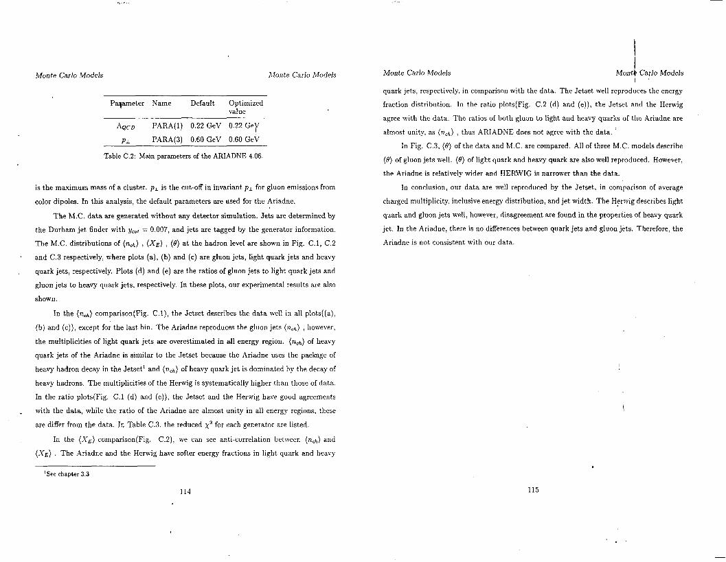
Monte Carlo Models Monte Carlo Models
Paqameter Name Default Optimized value
AQCD
Pl
PARA(1) 0.22 GeV 0.22 Gey
PARA(3) 0.60 GeV 0.60 GeV
Table C.2: Main parameters of the ARIADNE 4.06.
is the maximum mass of a cluster. pl is the cut-off in invariant pl for gluon emissions from
color dipoles. In this analysis, the default parameters are used for the Ariadne.
The M.C. data are generated without any detector simulation. Jets are determined by
the Durham jet finder with ycul = 0.007, and jets are tagged by the generator information.
The M.C. distributions of (n,r,) , (XE) , (0) at the hadron level are shown in Fig. C.l, C.2
* and C.3 respectively, where plots (a), (b) and ( ) c are gluon jets, light quark jets and heavy
quark jets, respectively. Plots (d) and (e) are the ratios of gluon jets to light quark jets and
gluon jets to heavy quark jets, respectively. In these plots, our experimental results are also
shown.
In the (nh) comparison(Fig. C.l), the Jetset describes the data well in all plots((a),
(b) and (c)), except for the last bin. The Ariadne reproduces the gluon jets (n,,,) , however,
the multiplicities of light quark jets are overestimated in all energy region. (no) of heavy
quark jets of the Ariadne is similar to the Jetset because the Ariadne uses the package of
heavy hadron decay in the Jetset’ and (n,h) of heavy quark jet is dominated by the decay of
heavy hadrons. The multiplicities of the Herwig is systematically higher than those of data.
In the ratio plots(Fig. C.l (d) and (e)), the Jetset and the Herwig have good agreements
_ with the data, while the ratio of the Ariadne are almost unity in all energy regions, these
are differ from the data. In Table C.3, the reduced x2 for each generator are listed.
In the (XE) comparison(Fig. C.2), we can see anti-correlation between (rich) and
(Xc) The Ariadne and the Herwig have softer energy fractions in light quark and heavy
Monte Carlo Models Mont b Carlo Models
quark jets, respectively, in comparison with the data. The Jetset well reproduces the energy
fraction distribution. In the ratio plots(Fig. C.2 (d) and (e)), the Jetset and the Herwig
agree with the data. The ratios of both gluon to light and heavy quarks of the Ariadne are
almost unity, as (nc,,) : thus ARIADNE does not agree with the data.
In Fig. C.3, (t9) of the data and M.C. are compared. All of three M.C. models describe
(0) of gluon jets well. (0) of light quark and heavy quark are also well reproduced. However,
the Ariadne is relatively wider and HERWIG is narrower than the data.
In conclusion, our data are well reproduced by the Jetset, in comparison of average
charged multiplicity, inclusive energy distribution, and jet width. The Herwig describes light
quark and gluon jets well, however, disagreement are found in the properties of heavy quark
jet. In the Ariadne, there is no differences between quark jets and gluon jets. Therefore, the
ariadne is not consistent with our data.
‘See chapter 3.3
114 115
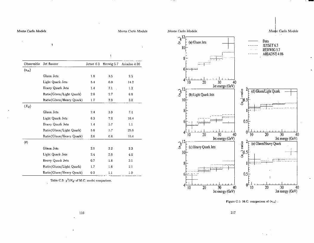
Monte Carlo Models Monte Carlo Models Monte Carlo Models
Observable Jet flavour Jetset 6.3 Herwig 5.7 Ariadne 4.OG
(%h)
Gluon Jets 1.8 3.5 2.5
Light Quark Jets 5.4 6.0 14.2
Heavy Quark Jets 1.4 7.1 1.2
Ratio(Gluon/Light Quark) 2.8 2.7 6.8
Ratio(Gluon/Heavy Quark) 1.7 2.8 3.0
txE) Gluon Jets 2.4 3.9 7.4
Light Quark Jets 6.3 7.0 16.4
Heavy Quark .Jets 1.4 5.7 1.1
Ratio(Gluon/Light Quark) 5.6 5.7 25.6
Ratio(Gluon/Heavy Quark) 3.6 6.6 10.4
(0)
Glaon Jets 2.1 2.2 2.3
^,12 Jet energy (GeV
0 5 (b) Light Quark Jets
8
4 tI;II Ill III11 IIll 10 20 30 40
512 Jet energy (GeV)
0 5 (c) Heavy Quark Jets
Light Quark Jets 2.4 2.0
Heavy Quark Jets 0.7 1.8
Ratio(Gluon/Light Quark) 1.7 1.6
Ratio(Gluon/Heavy Quark) 0.3 1.1
Table C.3: x2/N*, of M.C. model comparison.
4.0
3.1
2.1
1.9
lo-
4 I 111l1111111~~ 10 20 30 40
Jet energy (GeV)
- Data - - - - - JETSET 6.3
.... HERWK 5.7 - - - -.- ARIADNE 4.06
.z 2 I (d) Gluon/Light Quark I -
3.5: -5
0.5 :
I I I I I I I I I I I I I I I O 10 20 30 40
,Jet energy (GeV) .z 2 - (e) GluonMeavy Quark
+.51 5 -
0.5 ; I
I, I I I I B I I I I I I I I O 10 20 30 40
Jet energy (GeV)
116 117
Figure C.l: M.C. comparison of (&h)
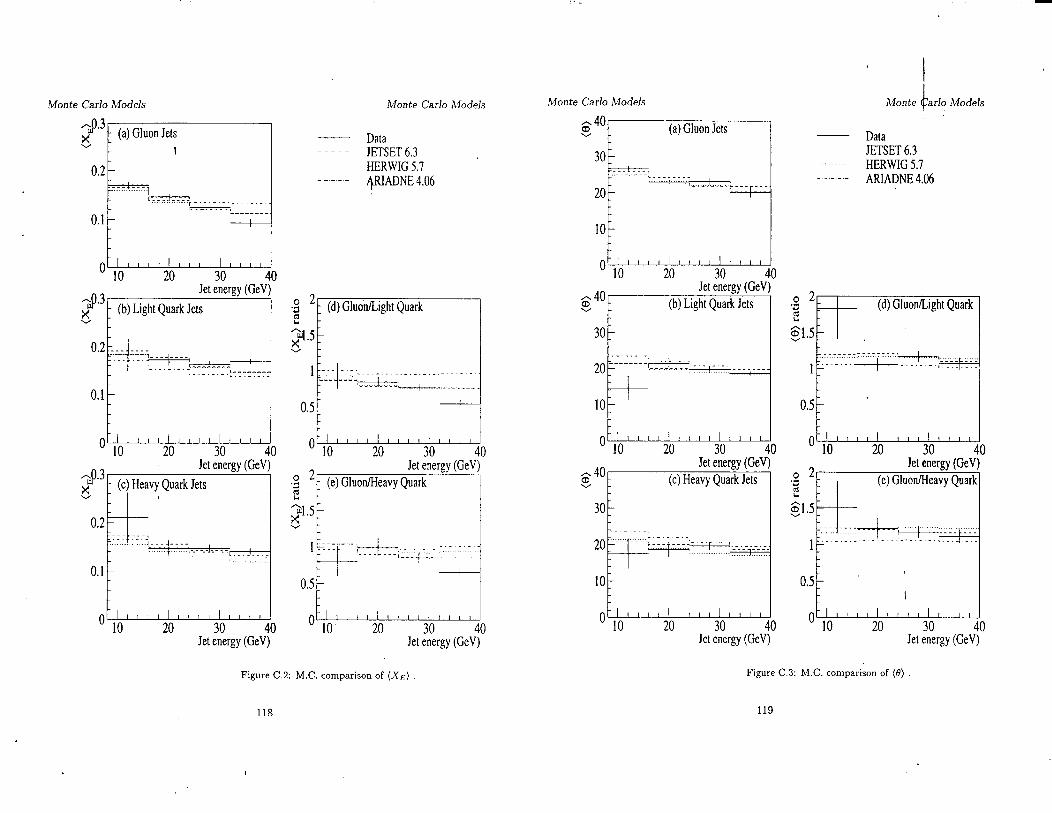
I .
OpoJ (&)
d

Monte Carlo Models Monte Carlo Models
120
Appendix D
Quark jet purity of the highest
energy jet
In chapter 5.2, we assume that the highest energy jet in a 3-jet event is a quark jet. This is
due the bremsstrahlung nature of gluon radiation. This natural assumption is used in the
selection of three jet samples: the gluon tagged, the light mixture, and the heavy mixture.
In this appendix, we consider the quark jet purity of the highest energy jet in 3-jet events.
Fig. D.l shows the energy spectra of jet 1, jet 2, and jet 3 in 3-jet events. The jets
are ordered by a kinetic jet energy(see chapter 5.1). In the jet energy range from 30 GeV
to 45 GeV, the energy spectra of jet 1 and jet 2 overlap. Thus, there is an ambiguity in I
the determination of the highest energy jet in the energy range due to a small jet energy
difference and finite jet energy resolution. However, events including such jet 1 and jet 2
are symmetric or nearly symmetric, and have a third jet with small jet energy. Such a jet
with small jet energy may be a gluon jet, and thus two higher energy jets can be quark jets.
Therefore, we consider that the jet energy overlap of jet 1 and jet 2 are not significant for the
assumption. In Fig. D.l, gluon components obtained by the Monte Carlo are also plotted.
The purity of quark jet in the highest energy jet is 93.5X, and the gluon contamination is
6.5%.
In order to estimate quark jet purity of the highest energy jet in data, we use the jet
121
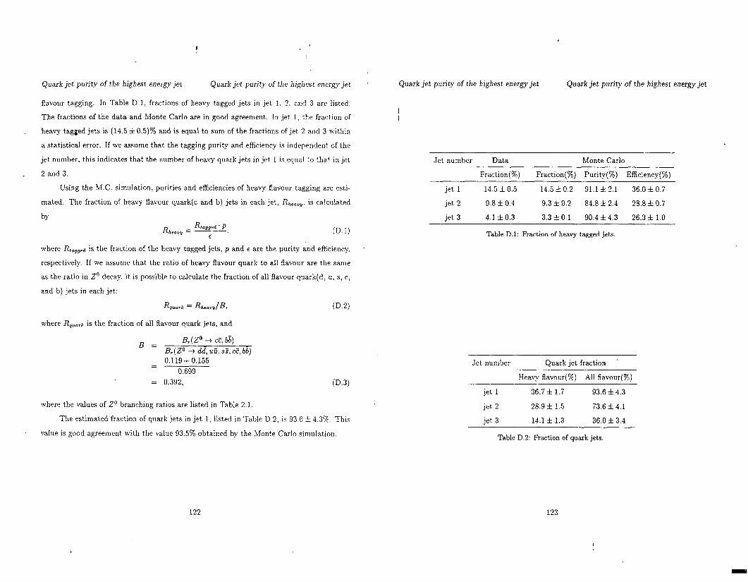
Quark jet purity of the highest energy jet Quark jet purity of the highest energy jet
flavour tagging. In Table D.l, fractions of heavy tagged jets in jet 1, 2. and 3 are listed.
The fractions of the data and Monte Carlo are in good agreement. In jet 1. the fraction of
heavy tagged jets is (14.5 + 0.5)% and is equal to sum of the fractions of jet 2 and 3 within
a statistical error. If we assume that the tagging purity and efficiency is independent of the
jet number, this indicates that the number of heavy quark jets in jet 1 is equal to that in jet
2 and 3.
Using the M.C. simulation, purities and efficiencies of heavy flavour tagging are esti-
mated. The fraction of heavy flavour quark(c and b) jets in each jet, Rhenvy, is calculated
by
0.1)
where Rtagged is the fraction of the heavy tagged jets, p and E are the purity and efficiency,
respectively. If we assume that the ratio of heavy flavour quark to all flavour are the same
as the ratio in 2’ decay, it is possible to calculate the fraction of all flavour quark(d, u, s, c,
and b) jets in each jet:
R guarlr = RtwaayjB~ (D.2)
where &,,.A is the fraction of all flavour quark jets, and
B= B, ( Z” -+ c?, b6)
B,(ZO --f dc?, uii, ss, d, bb) 0.119 + 0.155 =
0.699 = 0.392, (D.3)
where the values of Z” branching ratios are listed in Table 2.1.
The estimated fraction of quark jets in jet 1, listed in Table D.2, is 93.6 f 4.3%. This
value is good agreement with the value 93.5% obtained by the Monte Carlo simulation
Quark jet purity of the highest energy jet Quark jet purity of the highest energy jet
Jet number Data Monte Carlo
Fraction(%) Fraction(%) Purity(%) Efficiency(%)
jet 1 14.5 f 0.5 14.5 z! 0.2 91.1 f 2.1 36.0 f 0.7
jet 2 9.8 It 0.4 9.3 It 0.2 84.8 f 2.4 28.8 * 0.7
jet 3 4.1 zt 0.3 3.3 f 0.1 90.4 f 4.3 26.3 f 1.0
Table D.l: Praction of heavy tagged jets.
Jet number Quark jet fraction (
Heavy flavour(%) All flavour(%)
jet 1 36.7 f 1.7 93.6 f 4.3
jet 2 28.9 f 1.5 73.6 z!r 4.1
jet 3 14.1 f 1.3 36.0 It 3.4
Table D.2: Fraction of quark jets.
122 123
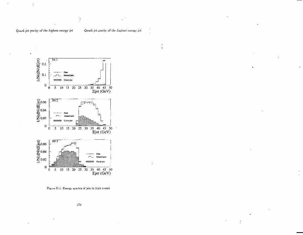
-.
i e
7 f L
m
0