Embed Size (px)
Citation preview
Clemson UniversityTigerPrints
All Dissertations Dissertations
8-2014
APPLICATION OF MODERN STATISTICALTOOLS TO SOLVING CONTEMPORARYECONOMIC PROBLEMS: EVALUATION OFTHE REGIONAL AGRICULTURALCAMPAIGN IMPACT AND THE USDAFORECASTING EFFORTSRAN XIEClemson University, [email protected]
Follow this and additional works at: https://tigerprints.clemson.edu/all_dissertations
Part of the Agricultural Economics Commons
This Dissertation is brought to you for free and open access by the Dissertations at TigerPrints. It has been accepted for inclusion in All Dissertations byan authorized administrator of TigerPrints. For more information, please contact [email protected].
Recommended CitationXIE, RAN, "APPLICATION OF MODERN STATISTICAL TOOLS TO SOLVING CONTEMPORARY ECONOMICPROBLEMS: EVALUATION OF THE REGIONAL AGRICULTURAL CAMPAIGN IMPACT AND THE USDAFORECASTING EFFORTS" (2014). All Dissertations. 1293.https://tigerprints.clemson.edu/all_dissertations/1293

i
APPLICATION OF MODERN STATISTICAL TOOLS TO SOLVING CONTEMPORARY ECONOMIC PROBLEMS: EVALUATION OF THE REGIONAL AGRICULTURAL CAMPAIGN IMPACT
AND THE USDA FORECASTING EFFORTS
A Dissertation Presented to
the Graduate School of Clemson University
In Partial Fulfillment of the Requirements for the Degree
Doctor of Philosophy Applied Economics
by Ran Xie
August 2014
Accepted by: Dr. Julia L. Sharp, Committee Chair
Dr. Olga Isengildina-Massa, Co-Chair Dr. David B. Willis
Dr. William C. Bridges Jr.
ii
ABSTRACT
The research is comprised with three studies to implement statistical tools for
examining two economic issues: the impact of a regional agricultural campaign on
participating restaurants and efforts of U.S. Department of Agriculture (USDA)
forecasting reports in agricultural commodity markets.
The first study examined how various components of the Certified South Carolina
campaign are valued by participating restaurants. A choice experiment was conducted to
estimate the average willingness to pay (WTP) for each campaign component using a
mixed logit model. Three existing campaign components—Labeling, Multimedia
Advertising, and the “Fresh on the Menu” program were found to have a significant
positive economic value. Results also revealed that the type of restaurant, the level of
satisfaction with the campaign, and the factors motivating participation significantly
affected restaurants’ WTP for the campaign components.
The second study evaluated the revision inefficiencies of all supply, demand, and
price categories of World Agricultural Supply and Demand Estimates (WASDE)
forecasts for U.S. corn, soybeans, wheat, and cotton. Significant correlations between
consecutive forecast revisions were found in all crops, all categories except for the seed
category in wheat forecasts. This study also developed a statistical procedure for
correction of inefficiencies. The procedure took into account the issue of outliers, the
impact of forecasts size and direction, and the stability of revision inefficiency. Findings
suggested that the adjustment procedure has the highest potential for improving accuracy
in corn, wheat, and cotton production forecasts.
iii
The third study evaluated the impact of four public reports and one private report
on the cotton market: Export Sales, Crop Processing, World Agricultural Supply and
Demand Estimates (WASDE), Perspective Planting, and Cotton This Month. The “best
fitting” GARCH-type models were selected separately for the daily cotton futures close-
to-close, close-to-open, and open-to-close returns from January 1995 through January
2012. In measuring the report effects, we controlled for the day-of-week, seasonality,
stock level, and weekend-holiday effects on cotton futures returns. We found statistically
significant impacts of the WASDE and Perspective Planting reports on cotton returns.
Furthermore, results indicated that the progression of market reaction varied across
reports.

iv
DEDICATION
This work is dedicated to the most important people in my life. God: thank you for your unreserved love and thank you for the wisdom you provide me to accomplish this work. My parents: thank you for your unconditional support with my studies. Thank you for your understanding and encouragement. My husband: thank you for your endurance and your constant love. Because of you, my life at Clemson is full of laughs! My church friends: I am so thankful for having you as my sisters and brothers. Thank you for your affirmation and prayers.

v
ACKNOWLEDGMENTS
I am truly thankful to my advisors Dr. Olga Isengildina-Massa and Dr. Julia Sharp
for allowing me to pursue this degree. They have been great mentors for guiding me
through my study at Clemson. Their encouragement and support have been great
motivation for pushing me forward, and I have benefited from them to be a better student
and a better person. I am also profoundly thankful to my committee members Dr. David
Willis and Dr. William Bridges for their time, dedication, and willingness to read this
document and provide valuable inputs.
I want to extend my gratitude to Dr. Carlos Carpio and Dr. Gerald Dwyer for their
interest and investment in my projects. Their expertise enabled me to accomplish my
work. Thanks especially to Steven MacDonald in USDA for providing research data and
answering research questions as an insider.
Throughout my time at Clemson, I have been benefited from the teaching of
several great professors. My sincere thanks go to Dr. James Rieck, Dr. Patrick Gerald,
Dr. Kevin Tsui, and Dr. Paul Wilson. I would be remiss to not acknowledge Dr.
Martinez-Dawson and Dr. Richard Dubsky for helping me to become a successful course
instructor.
Lastly, I want to thank my fellow graduate students and friends for their kindness
and understanding. They truly enhanced my experience at Clemson.
vi
TABLE OF CONTENTS
Page
TITLE PAGE .................................................................................................................... i ABSTRACT ..................................................................................................................... ii DEDICATION ................................................................................................................ iv ACKNOWLEDGMENTS ............................................................................................... v LIST OF TABLES ........................................................................................................ viii LIST OF FIGURES ......................................................................................................... x CHAPTER I. INTRODUCTION ......................................................................................... 1 Overview and Objectives ......................................................................... 1 References ................................................................................................ 4
II. VALUATION OF VARIOUS COMPONENTS OF A REGIONAL PROMOTION CAMPAIGN BY PARTICIPATING RESTAURANTS ...................................................... 5
Introduction .............................................................................................. 5 Data and Methods .................................................................................... 8 Results .................................................................................................... 16
Summary and Conclusions .................................................................... 23 References .............................................................................................. 25
III. ARE REVISIONS OF USDA’S COMMODITY FORECASTS EFFICIENT? .................................................................. 36 Introduction ............................................................................................ 36 Data ........................................................................................................ 38 Methods.................................................................................................. 41 Results .................................................................................................... 49
Summary and Conclusions .................................................................... 59 References .............................................................................................. 62
vii
Table of Contents (Continued)
Page
IV. QUANTIFYING PUBLIC AND PRIVATE INFORMATION EFFECTS ON THE COTTON MARKET ............................................................................................... 81 Introduction ............................................................................................ 81 Data ........................................................................................................ 84 Methods.................................................................................................. 90 Results .................................................................................................... 98
Summary and Conclusions .................................................................. 106 References ............................................................................................ 109
V. DISSERTATION SUMMARY ................................................................. 126
viii
LIST OF TABLES
Table Page 2.1 Description of Variables Included in the OLS Method ............................... 28 2.2 Summary Statistics Describing the Characteristics of Restaurants Participating in the Certified South Carolina Campaign “Fresh on the Menu” Program .............................. 29 2.3 Summary Statistics Describing the Perceived Effects of Restaurant Participation in the Certified South Carolina Campaign “Fresh on the Menu” Program .............................. 31 2.4 Mixed Logit Estimates ................................................................................. 33 2.5 Comparison of Population Parameters and Means of Individual Parameters ............................................................................ 33 2.6 The Effects of Participating Restaurant Characteristics on Their Individual WTP for Four Campaign Components ........................................................................................... 34 3.1 Tests of Revision Efficiency for WASDE Corn Forecasts, 1984/85-2011/12 Marketing Years ........................................................ 65 3.2 Tests of Revision Efficiency for WASDE Soybean Forecasts, 1984/85-2011/12 Marketing Years ....................................... 66 3.3 Tests of Revision Efficiency for WASDE Wheat Forecasts, 1984/85-2011/12 Marketing Years ....................................... 67 3.4 Tests of Revision Efficiency for WASDE Cotton Forecasts, 1984/85-2011/12 Marketing Years ....................................... 68 3.5 Evaluation of Revision Inefficiency Correction Procedures for Corn Forecasts ............................................................... 69 3.6 Evaluation of Revision Inefficiency Correction Procedures for Soybean Forecasts ......................................................... 70 3.7 Evaluation of Revision Inefficiency Correction Procedures for Wheat Forecasts ............................................................. 71
ix
List of Tables (Continued) Table Page 3.8 Evaluation of Revision Inefficiency Correction Procedures for Cotton Forecasts ............................................................ 72 3.9 Evaluation of the New Revision Inefficiency Correction Procedure over Time for Corn Forecasts ............................................... 73 3.10 Evaluation of the New Revision Inefficiency Correction Procedure over Time for Soybean Forecasts ......................................... 74 3.11 Evaluation of the New Revision Inefficiency Correction Procedure over Time for Wheat Forecasts ............................................. 75 3.12 Evaluation of the New Revision Inefficiency Correction Procedure over Time for Cotton Forecasts ............................................ 76 4.1 New York Board of Trade (NYBOT) Cotton No. 2 Futures Contracts with Each Report Release Month ........................... 113 4.2 Descriptive Statistics for Cotton Daily Futures Returns, January 1995-January 2012 ................................................................. 113 4.3 Test Statistics of Model Selection for Cotton Daily Futures Returns, January 1995-January 2012 ...................................... 114 4.4 Results for Cotton Daily Futures Close-to-Close Returns, January 1995-January 2012 ................................................................. 116 4.5 Impact of Reports on Conditional Standard Deviation of the Daily Cotton Futures Close-to-Close Returns, January 1995-January 2012 ................................................................. 118 4.6 WASDE and Prospective Planting Reports Effect in Context ................................................................................................. 118 4.7 Final Results for Cotton Daily Futures Returns, January 1995-January 2012 ............................................................................... 119
x
LIST OF FIGURES
Figure Page 2.1 Example of One of the Scenarios from the Restaurant Survey .................................................................................................... 35 2.2 Box Plot of WTP for LABEL, SIGNAGE, MULTI, and FOTM .............................................................................................. 35 3.1 The WASDE Forecasting Cycle for Corn, Soybeans, Cotton and Wheat Relative to the 2011/12 U.S. Marketing Year ...................................................................................... 77 3.2 Corn and Soybean Production Forecasting Cycle and Corresponding Revision Cycle for a Marketing Year ........................... 78 3.3 An Example of Outlier Detection For Corn Production using the October Data from 1984/95 to 2002/03 ................................. 78 3.4 Stability of Revision Inefficiency Over Time: Corn Production .............................................................................................. 79 3.5 Structural change test (QLR) for corn production: 1984/85-2011/12 .................................................................................... 80 4.1 Cotton Daily Futures Returns, January 1995-Janaury 2012 ...................... 121 4.2 Cotton Daily Futures Squared Returns, January 1995- Janaury 2012 ........................................................................................ 122 4.3 Quantile and Quantile Plot of GARCH(1,1)-normal, GARCH(1,1)-t, and IGARCH(1,1)-t models for Cotton Daily Futures Close-to-Close Returns, January 1995-Janaury 2012 ................................................................. 123 4.4 The Autocorrelations (ACF) and Partial Autocorrelations (PACF) Plots of the Squared Close-to-Close Returns, January 1995-Janaury 2012 ................................................................. 124 4.5 Monthly Effects of WASDE Reports on Cotton Daily Futures Close-to-Close Returns, January 1995- Janaury 2012 ........................................................................................ 124
xi
List of Figures (Continued) Figure Page 4.6 Progression of Market Reaction to WASDE, Prospective Planting, Cotton This Month Reports in Cotton Daily Futures Close-to-Close, Close-to-Open, and Open-to-Close Returns, January 1995-Janaury 2012 .......................... 125
1
CHAPTER ONE
INTRODUCTION
Overview and Objective
The current research aims to implement statistical tools for examining two
economic issues: the impact of a regional agricultural campaign on participating
restaurants and efforts of U.S. Department of Agriculture (USDA) forecasting reports in
agricultural commodity markets. Both the campaign and the forecasts are supported by
governmental funding. Given the current market environment that federal and state
budgets have been gradually pruned, addressing these two issues will help government
officials to justify the expenditure of public funds. This research comprises three
manuscripts including 1) the examination of the Certified South Carolina campaign, 2)
the evaluation of accuracy and efficiency of the World Agricultural Supply and Demand
Estimates (WASDE), a forecasting report by the U.S. Department of Agriculture
(USDA), and 3) the assessment of public and private information effects on the cotton
market.
In the United States, regional agricultural campaigns, which promote locally
grown products, have grown rapidly since the mid-1990s; by 2010, all 50 states had such
campaigns in place (Onkenand Bernard, 2010). The Certified South Carolina campaign
was launched on May 22, 2007. The “Fresh on the Menu” component, which promotes
local restaurants preparing dishes with “Certified South Carolina” products, was added in
February 2008. Most previous studies (e.g. Carpio and Isengildina-Massa, 2010;
Patterson et al., 1999) analyzed the impact of locally grown campaigns focusing
2
exclusively on the benefits received by farmers, while the impact of such campaigns on
local restaurants had been neglected. The objective of the first study is to examine the
perceived economic value of various components of the Certified South Carolina
campaign by the generally overlooked segment of participating restaurants and to explore
the relationship between campaign valuation and characteristics of participating
restaurants. This study is described in Chapter 2.
Industry participants have relied on USDA forecasts to make production,
marketing processing, and retailing decisions for many years. Recently, there have been
concerns about the accuracy of USDA estimates. Releasing an incorrect forecast will
mislead the markets and cause unnecessary price movements. In addition, errors in
USDA price estimates may result in large changes in the payments to agricultural
producers since some government payments are computed using these estimates
(Isengildina-Massa, Karali, and Irwin, 2013). The USDA actually warns readers that its
estimates are subject to revisions and sampling errors. The objective of the second study
is to evaluate the monthly revision efficiency of all supply, demand, and price categories
for U.S. corn, soybean, wheat, and cotton forecasts, published in the monthly WASDE
reports, which are viewed as some of the most influential public reports. In addition, a
statistical model is developed in this study, which takes into account outlier adjustment,
the impact of other variables on inefficiency, and structural changes to correct for
inefficiency and therefore improve the accuracy of WASDE forecasts. This study is
described in Chapter 3.
3
The National Agricultural Statistics Service, part of the USDA, has a $156.8m
budget for approximately 500 reports each year and 1,050 employees (Meyer, 2011).
There is no doubt that releases of USDA reports move the markets. However, most
previous studies evaluating the impact of USDA forecasting reports concentrated on one
report at a time. In addition, while the USDA Crop Production, the World Agricultural
Supply and Demand Estimates (WASDE), and other reports have been evaluated, the
influences of many other reports, such as the Crop Process and Perspective Plantings,
have been neglected. Furthermore, while we know which reports affect corn, soybean,
wheat, livestock and hog markets, other commodities have been overlooked. Therefore,
the objective of the third study is to estimate the impact of all major public and private
reports on the cotton market. In measuring the report effects, we control for the day-of-
week, seasonality, stock level, and weekend-holiday effects on cotton futures returns.
This study is described in Chapter 4.
Chapter 5 summarizes the results from all three studies.
4
References
Carpio, C.E., and O. Isengildina-Massa. “To Fund or Not to Fund: Assessment of the Potential Impact of a Regional Promotion Campaign.” Journal of Agricultural and Resource Economics 35(August 2010):245-60.
Isengildina, O., B. Karali, S.H. Irwin. “When do the USDA forecasters make mistakes?” Applied Economics 45(2013):5086-5103.
Meyer, G. Reliability of US Crop Reports Questioned. Financial Times, July 12, 2011.
Onken, K.A., and J.C. Bernard. “Catching the ‘Local’ Bug: A Look at State Agricultural Marketing Programs.” Choices 25(2010):1-7.
Patterson, P.M., H. Olofsson, T.J. Richards, and S. Sass. “An Empirical Analysis of State Agricultural Product Promotions: A Case Study on Arizona Grown.” Agribusiness 15(1999):179-96.
5
CHAPTER TWO
VALUATION OF VARIOUS COMPONENTS OF A REGIONAL PROMOTION
CAMPAIGN BY PARTICIPATING RESTAURANTS
Introduction
Government funded advertising campaigns play an important role in agricultural
and food policy around the world. In the United States, regional promotion programs
have grown rapidly since the mid-1990s. The number of states conducting such programs
increased from 23 to 43 between 1995 and 2006 (Patterson, 2006), and by 2010 all 50
states had such programs in place (Onken and Bernard, 2010). Previous studies
evaluating regional promotion campaigns showed mixed evidence regarding campaign
effectiveness (e.g. Carpio and Isengildina-Massa, 2010; Govindasamy et al., 2003;
Patterson et al., 1999). Govindasamy et al. (2003) found that the Jersey Fresh program
generated about $32 of returns for fruit and vegetable growers for every dollar invested.
In other words, the $1.16 million campaign generated $36.6 million in sales for New
Jersey produce growers and a total economic impact for the state economy of $63.2
million in 2000. Carpio and Isengildina-Massa (2010) concluded that the Certified South
Carolina campaign generated a return on investment of 618% or a benefit-cost
(producers benefit / state government expenses) ratio of 6.18 in 2007. In contrast,
Patterson (1999) found little evidence of an increase in local product sales due to the
Arizona Grown campaign.
Most previous studies analyze the impact of the locally grown campaigns
focusing exclusively on benefits received by farmers (e.g., Carpio and Isengildina-Massa,
6
2010; Patterson et al., 1999). While farmers tend to be the primary beneficiaries of such
campaigns, their benefits extend far beyond and include consumers, restaurants and
farmers’ markets as well as the secondary effects on the rest of the economy
(Govindasamy et al., 2003; Carpio and Isengildina-Massa, 2013). To the best of our
knowledge, no studies of the impact of such campaigns on local restaurants have been
conducted to date. Ignoring these additional effects of locally grown campaigns would
lead to an underestimation of their impact, especially in cases where some of the
campaign components focus exclusively on restaurants. Additionally, regional promotion
campaigns have typically been analyzed as a whole, providing little guidance to policy
makers about the value of separate campaign components. Given these limitations, the
goals of the current study are twofold: 1) to examine the perceived economic value of
various components of the Certified South Carolina campaign by the generally
overlooked segment of participating restaurants, and 2) to explore the relationship
between campaign valuation and characteristics of participating restaurants.
The Certified South Carolina campaign was launched on May 22, 2007 and was
financed by special appropriations from the state legislature. The goal of the campaign
was to increase consumer demand for the state produced food products and increase
agribusiness profitability. Annual campaign expenditures averaged about $1.3 million
during 2007-2010. Original campaign components included the design and distribution of
labels and signage for “Certified South Carolina” products and advertisement of South
Carolina food products on television, radio, magazines, newspapers and billboards. The
“Fresh on the Menu” component, which promotes local restaurants preparing dishes with
7
“Certified South Carolina” products, was added in February 2008. In order to enroll into
this free program, restaurants needed to complete an application form, pledging to offer a
menu that includes at least twenty-five percent “Certified South Carolina” products such
as fresh fruits, vegetables, meats and seafood as available in season. Participating
restaurants take advantage of the South Carolina Department of Agriculture’s (SCDA)
multimedia advertising and branding efforts, including kits and artwork for logos and
online, radio, magazine, newspaper, and billboard advertisement promotions. When it
was first introduced in 2008, 180 restaurants signed up for the “Fresh on the Menu”
program. By July 2010, when the data for this study was collected, the campaign
membership had increased to 288 restaurants.
Since restaurants are not required to pay a participation fee for the campaign, this
study used a choice-based conjoint analysis method to determine the perceived economic
value that participating restaurants place on each campaign component. The data
generated from a discrete choice experiment were analyzed using a mixed logit model,
allowing us to estimate participating restaurants’ average willingness to pay (WTP) for
each of the campaign components, which represents their respective economic values
(Holmes and Adamowicz, 2003). In addition to the average WTP estimates for each
campaign component, we estimated individual level WTP values which are in turn used
as dependent variables in linear regression models to uncover how individual WTP for
each component is affected by participating restaurants’ characteristics. The findings of
this study could help policy makers and marketers determine which campaign
components are more effective and could be used to guide future campaign fund
8
allocations. In an environment of decreasing state and federal funding it becomes
increasingly important to have specific estimates of the effectiveness of alternative
campaign investments.
Data and Methods
Survey Approach
The data used for estimation in this study were collected via a survey of the
managers of 288 restaurants that participated in the South Carolina “Fresh on the Menu”
in July 2010. The survey was administered through a combination of internet (Qualtrics)
and mail1 and included the entire population of participating restaurants. Every effort was
made to obtain the highest possible response rate including the use of economic
incentives, an invitation letter, the shortest possible survey instruments pre-tested using
focus groups; the use of the Dillman survey method (with two reminders after the first (e-
)mailing); and the use of a mail survey to complement online surveys. The survey
generated 71 usable observations for a response rate of about 25%, which is relatively
high compared to a 13.4% average response rate in a study of 199 online surveys
conducted by Hamilton (2003)2. In order to assess the representativeness of our sample,
we compared the location of the restaurants in the population with that of the sample
(location was the only known characteristic of the population). The proportion of 1 The results of this study were not statistically different across the two survey formats. 2 Although the relationship between low response rates and low survey accuracy has been 2 Although the relationship between low response rates and low survey accuracy has been academically debated for a long time, several recent studies suggest a very weak or non-existent relation between the two (Keeter et al., 2000; Curtin et al., 2000; Brick et al., 2003; Keeter et al., 2006; Holbrook et al., 2008). !
9
restaurants from each region in the sample generally followed the corresponding
proportion in the population except for one of ten regions considered: the Berkerly-
Charleston-Dorchester whose proportion in the sample (16.4%) was lower than the
proportion in the population (30.9%).3
Choice Experiment
Various methods are available to elicit and estimate preferences for products or
services or the value of changes in the qualities of existing products. These methods
include choice experiments (e.g., Adamowicz et al., 1998; Louviere, Hensher, and Swait,
2000), dichotomous choice questions (e.g., Hanemann, Loomis, and Kanninen, 1991;
Ready, Buzby, and Hu, 1996), and experimental auctions (e.g., Lusk et al., 2001; List and
Shogren, 1998). Choice-based conjoint analysis or choice experiments (CE) have the
advantage of closely mirroring typical choice experience--making one decision over
several options--and allowing a researcher to estimate the trade-offs between several
competing product attributes (Lusk and Hudson, 2004). Additionally, CE are easier to
organize with no requirement for laboratory sessions and the need of an actual product
(which is not realistic in the context of this project). Several studies also prove that
hypothetical responses to CE are very consistent with revealed preferences (e.g., Carlsson
and Martinsson, 2001; Adamowicz et al., 1997).
CE are firmly rooted in the economic theory that the decision making process can
3 A weighted maximum likelihood estimator was also used to explore the robustness of the results to the difference between the sampling and population proportions (Cameron and Trivedi, 2005). All the estimated coefficients were similar and had overlapping 95% confidence intervals except for the mean coefficient for SIGNAGE. This coefficient was significant in the model using weights. !
10
be viewed as a comparison of indirect utility functions and analyzed within the random
utility framework (McFadden, 1974). The data obtained from CE can then be analyzed
using discrete choice models and the results can be used to estimate WTP values for the
various attributes of the good or product under study (Alfnes et al., 2006; Holmes and
Adamowicz, 2003; Revelt and Train, 1998). In this study we use CE to examine
restaurant managers’ preferences for each of the attributes (components) of the Certified
South Carolina campaign. Thus restaurant managers are considered the consumers of the
regional promotion campaign and choose the campaign profile (combination of various
components) that allows them to reach the highest level of utility. Accordingly, the value
of the campaign can be measured as the maximum amount of money restaurants would
be willing to pay for a certain campaign profile. This approach allows us to estimate the
economic value of the campaign, which is currently offered to participants free of charge.
In order to determine the perceived economic value of each component of the
Certified South Carolina campaign, the CE design incorporated four attributes
corresponding to the components of the existing campaign: (1) Labeling (LABEL) which
provides labels for “Certified South Carolina” products; (2) Point of Purchase Signage
(SIGNAGE) which provides “Certified South Carolina” signs at food buying locations,
such as supermarkets, farmers markets, and roadside stands; (3) Multimedia Advertising
(MULTI), which funds television, radio, magazine, newspaper, and billboard
advertisements promoting “Certified South Carolina” products; and (4) the “Fresh on the
Menu” component (FOTM) which promotes local restaurants preparing and selling menu
items that include “Certified South Carolina” products in season. Each choice was

11
associated with one of two payment methods (METHOD): membership fee or donation.
These two options were selected because they are the most widely used methods for
funding public and private programs that promote locally grown products. The payment
amount was also added so that the WTP for each campaign component could be
calculated. A pilot study of four randomly selected restaurants in the upstate region of
South Carolina was conducted to determine the appropriate bid vector (following
Ratcliffe, 2000). The payment levels (PAY) were identified as $20, $50, $100, $150, and
$200. The combination of all the attributes and levels resulted in a total of 160
(2*2*2*2*2*5) possible campaign profiles and a full factorial design consisting of 12,720
(C2160) possible choices. However, it was not feasible to include such a large number of
scenarios in a CE. Hence, a fractional factorial design was applied to choose 18 scenarios
by comparing the D-Efficiency of each combination. Having 18 scenarios within a single
survey was still considered excessive. Therefore, the design was blocked into three
versions of the questionnaire where each respondent was offered 6 scenarios with trinary
choices. A series of SAS Macro programs were used to first generate the campaign
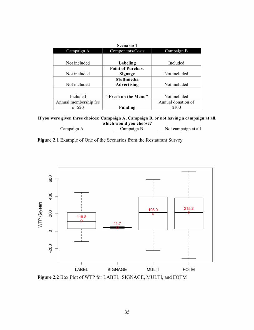
profiles and then to construct the CE used in this study. Figure 2.1 provides an example
of one of the 18 scenarios. In each case, the manager of the restaurant was asked to
choose from campaign A, B, or no campaign at all with two types of funding and 5
different funding levels. Having these options allowed the experimental design to fit an
actual market situation without “forcing” a choice (Louviere, Hensher, and Swait, 2000).
Average WTP Estimation, Mixed Logit Model
The econometric choice model used in this study is the random parameter/mixed

12
logit model4 developed by Revelt and Train (1998). The mixed logit model was chosen
because it allows efficient estimation of repeated choices by the same respondent within
choice-based conjoint experiments. Moreover, this model relaxes the restrictive
assumptions of the conditional logit model (Revelt and Train, 1998).
Following Revelt and Train (1998), the random utility function of restaurant
managers (Uni) is assumed to be comprised of a systematic ( ) and a random ( )
component:
(2.1) , i=1,…,I, , and n=1,…,N,
where Uni is the true but unobservable indirect utility of restaurant n associated with
campaign profile i. A restaurant chooses alternative i from choice set C only if ,
where n=1,…, N, alternative and . Accordingly, choices are made based on
utility differences across alternatives and the probability of choosing i can be expressed
as:
(2.2) .!
In this study, restaurant managers need to make six choices in a row, so choice
situations are defined using the index t (t=1, …, 6). Moreover, the indirect utility that
restaurant manager n expects to obtain from alternative i in choice situation t is assumed
to be linear-in-parameters (Revelt and Train, 1998):
(2.3) ,
where coefficient vector βn is the unobserved preference parameter associated with 4 The results generated by applying a conditional logit model are available upon request.
vni εni
Uni = v ni+εni i∈C
Uni >Unj
i, j ∈C i ≠ j
P(i |C) = P(Uni >Unj ) = P(vni + εni > vnj + εnj ) = P(vni − vnj > εnj − εni )∀i, j ∈C, i ≠ j,n =1,...,N
Unit = βn' xnit + εnit
13
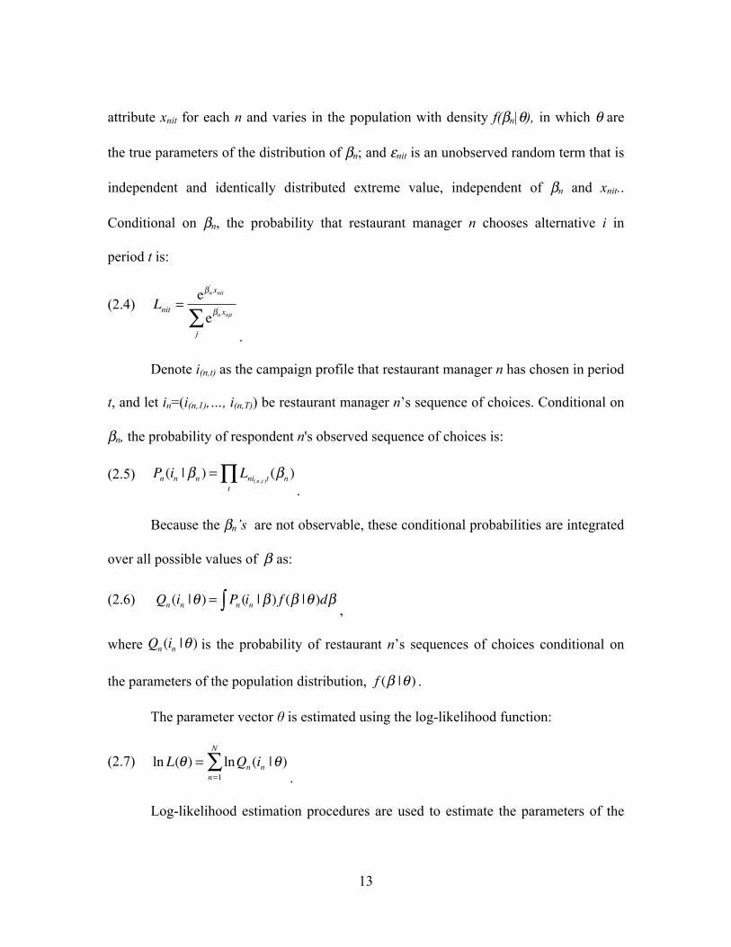
attribute xnit for each n and varies in the population with density f(βn|θ), in which θ are
the true parameters of the distribution of βn; and εnit is an unobserved random term that is
independent and identically distributed extreme value, independent of βn and xnit..
Conditional on βn, the probability that restaurant manager n chooses alternative i in
period t is:
(2.4)
.
Denote i(n,t) as the campaign profile that restaurant manager n has chosen in period
t, and let in=(i(n,1),…, i(n,T)) be restaurant manager n’s sequence of choices. Conditional on
βn, the probability of respondent n's observed sequence of choices is:
(2.5) .
Because the βn’s are not observable, these conditional probabilities are integrated
over all possible values of as:
(2.6) Qn (in |θ ) = Pn (∫ in | β ) f (β |θ )dβ ,
where is the probability of restaurant n’s sequences of choices conditional on
the parameters of the population distribution, .
The parameter vector θ is estimated using the log-likelihood function:
(2.7) .
Log-likelihood estimation procedures are used to estimate the parameters of the
Lnit =eβn
' xnit
eβn' xnjt
j∑
Pn (in | βn ) = Lni(n,t )t (βn )t∏
β
Qn (in |θ )
f (β |θ )
lnL(θ) = lnQn (in |θ)n=1
N
∑
14
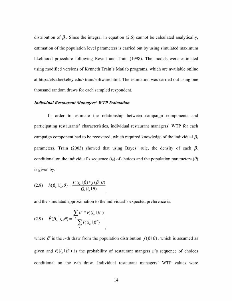
distribution of βn. Since the integral in equation (2.6) cannot be calculated analytically,
estimation of the population level parameters is carried out by using simulated maximum
likelihood procedure following Revelt and Train (1998). The models were estimated
using modified versions of Kenneth Train’s Matlab programs, which are available online
at http://elsa.berkeley.edu/~train/software.html. The estimation was carried out using one
thousand random draws for each sampled respondent.
Individual Restaurant Managers’ WTP Estimation
In order to estimate the relationship between campaign components and
participating restaurants’ characteristics, individual restaurant managers’ WTP for each
campaign component had to be recovered, which required knowledge of the individual βn
parameters. Train (2003) showed that using Bayes’ rule, the density of each βn
conditional on the individual’s sequence (in) of choices and the population parameters (θ)
is given by:
(2.8) ,
and the simulated approximation to the individual’s expected preference is:
(2.9)
,
where βr is the r-th draw from the population distribution f (β |θ ) , which is assumed as
given and is the probability of restaurant mangers n’s sequence of choices
conditional on the r-th draw. Individual restaurant managers’ WTP values were
h(βn | in,θ ) =Pn (in | β )* f (β |θ )
Qn (in |θ )
E(βn | in,θ ) =β r *Pn (in | β
r )r∑
Pn (in | βr )
r∑
Pn (in | βr )
15
WTPk =α k + βk,iMOTIVATION +i=1
4
∑ βk,5SATISFACTION + βk,iIMAGE +i=6
12
∑ βk,13SIZE + εk
k = LABEL,SIGNAGE,MULTI,FOTM
calculated using estimates of βn. The estimated parameters ! were used instead of the
population parameters θ.
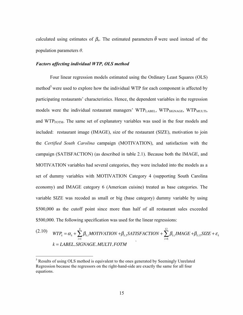
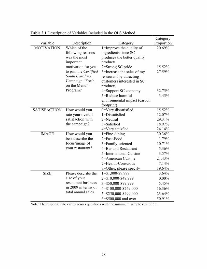
Factors affecting individual WTP, OLS method
Four linear regression models estimated using the Ordinary Least Squares (OLS)
method5 were used to explore how the individual WTP for each component is affected by
participating restaurants’ characteristics. Hence, the dependent variables in the regression
models were the individual restaurant managers’ WTPLABEL, WTPSIGNAGE, WTPMULTI,
and WTPFOTM. The same set of explanatory variables was used in the four models and
included: restaurant image (IMAGE), size of the restaurant (SIZE), motivation to join
the Certified South Carolina campaign (MOTIVATION), and satisfaction with the
campaign (SATISFACTION) (as described in table 2.1). Because both the IMAGE, and
MOTIVATION variables had several categories, they were included into the models as a
set of dummy variables with MOTIVATION Category 4 (supporting South Carolina
economy) and IMAGE category 6 (American cuisine) treated as base categories. The
variable SIZE was recoded as small or big (base category) dummy variable by using
$500,000 as the cutoff point since more than half of all restaurant sales exceeded
$500,000. The following specification was used for the linear regressions:
(2.10)
.
5 Results of using OLS method is equivalent to the ones generated by Seemingly Unrelated Regression because the regressors on the right-hand-side are exactly the same for all four equations. !
16
Results
Descriptive Analysis
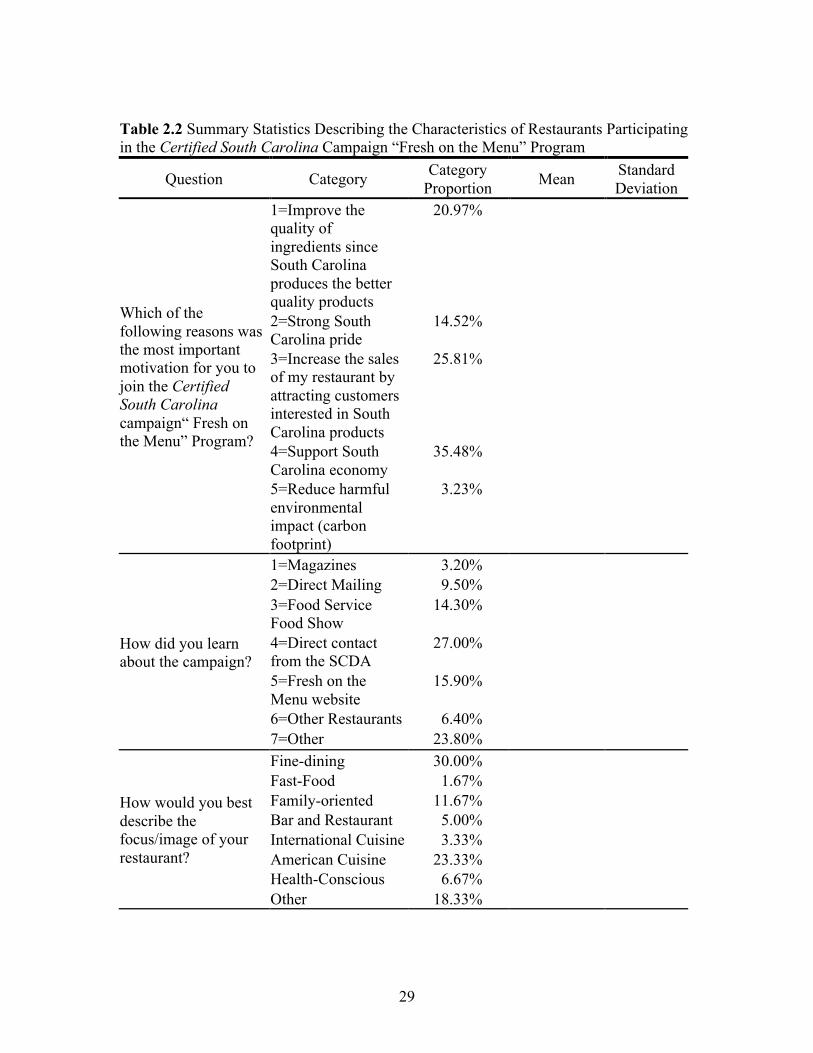
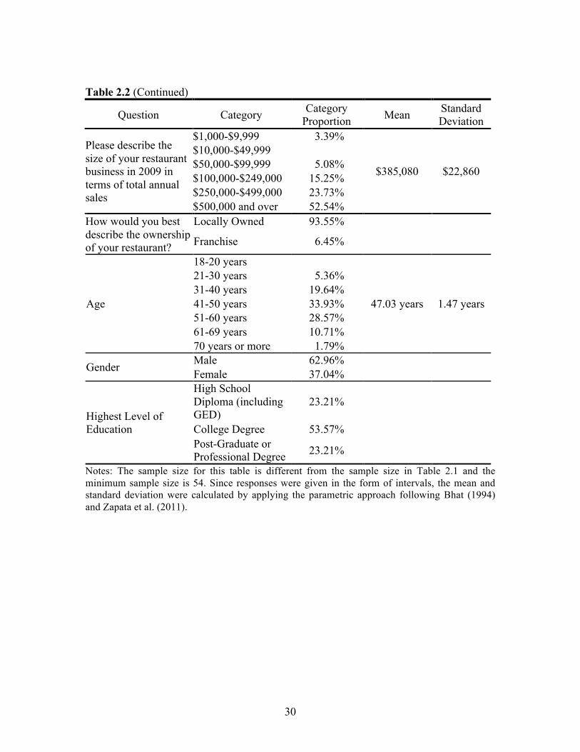
Table 2.2 presents selected descriptive statistics of the participating restaurants.
Almost all (94%) participating restaurants were locally owned. The largest response
category for the image of participating restaurants was fine dining (30%), followed by
American cuisine (23%). The average annual sales for year 2009 across all respondents
was $385,0806 with about half of the restaurants having sales over $500,000. The average
participating restaurant manager was 47 years old, male, with a college degree. The most
commonly mentioned motivation to participate in the campaign was to support the South
Carolina economy (35%) (similar to the findings for consumers reported by Carpio and
Isengildina-Massa, 2009), followed by a desire to increase sales by attracting customers
interested in South Carolina products (26%), and to improve the quality of ingredients
(since South Carolina products are believed to be of better quality) (21%). The most
frequent way respondents learned about the Certified South Carolina campaign “Fresh on
the Menu” program was through a direct contact from the SCDA (27%), followed by the
“Fresh on the Menu” website (16%), and food service shows (14%).
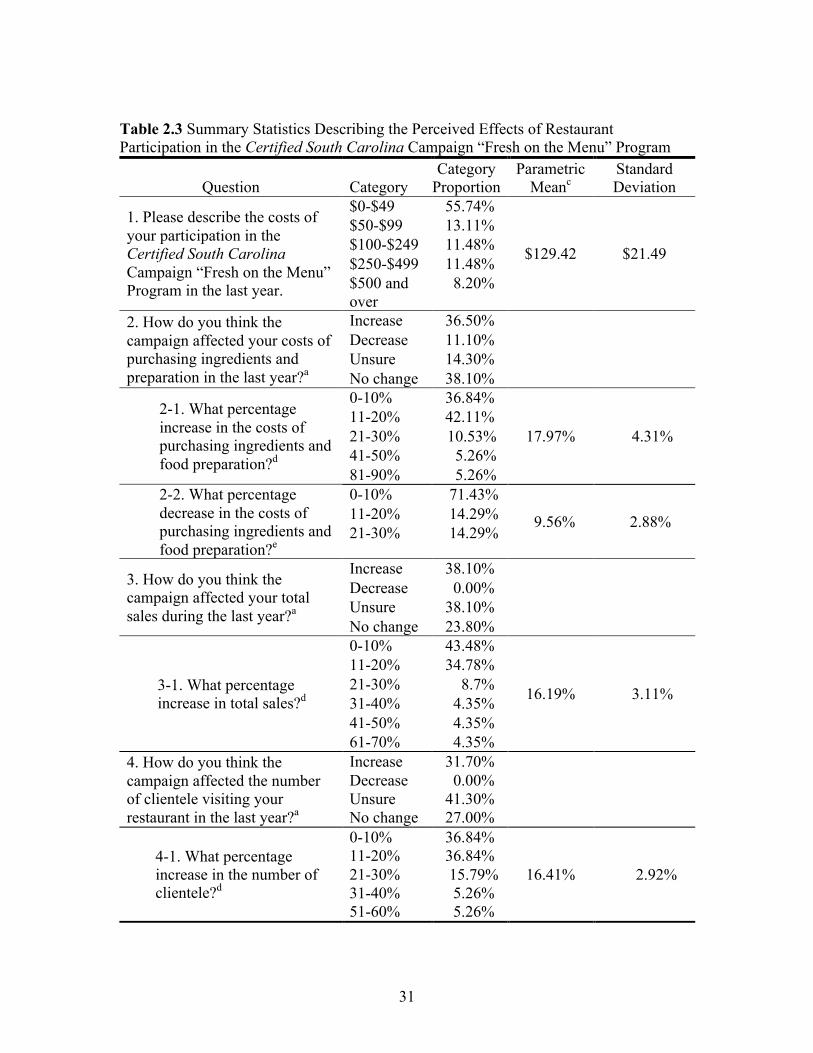
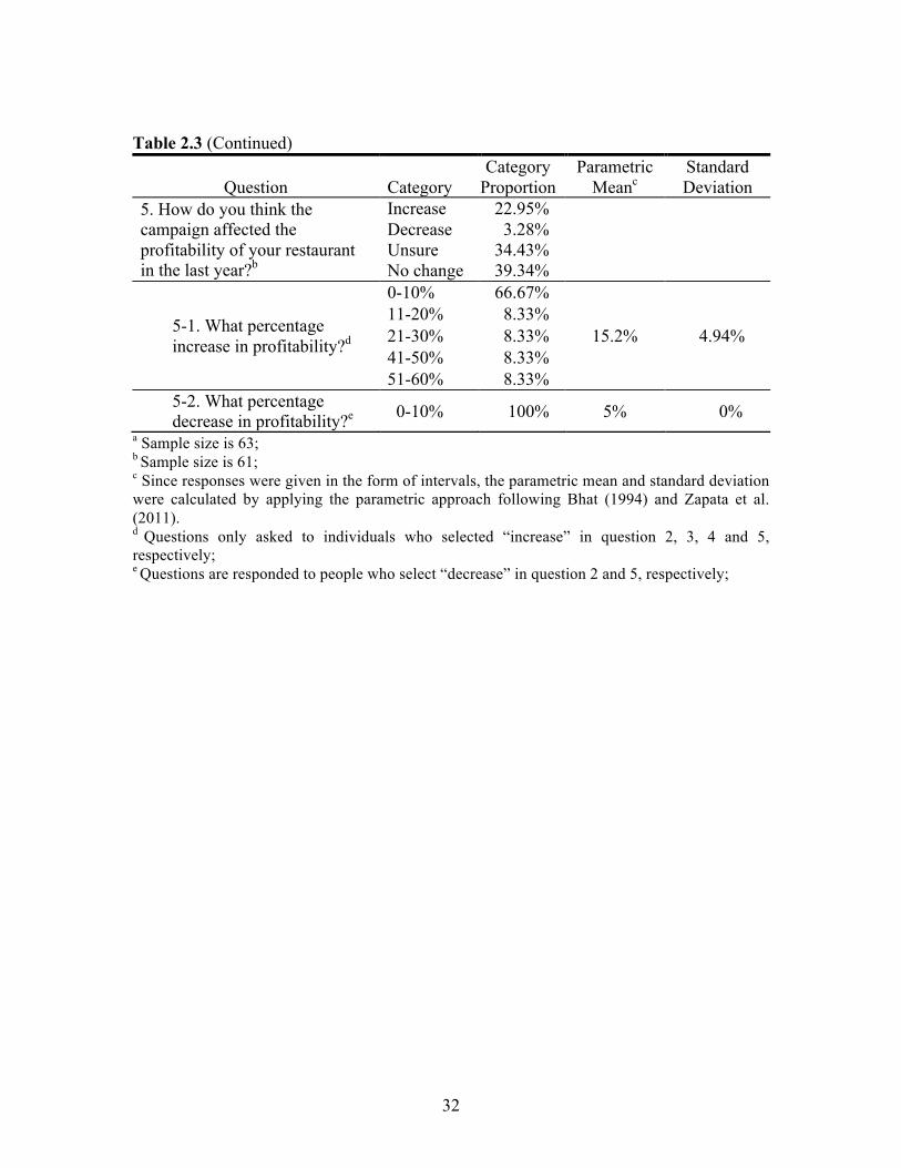
Perceived impacts of restaurant participation in the Certified South Carolina
campaign “Fresh on the Menu” program are described in table 2.3. About 38.1% of
respondents reported that their sales increased during the last year due to the campaign,
and the estimated average reported increase for this group was 16.2%. About 31.7% of
6 Since responses were given in the form of intervals, the means were calculated by applying a parametric approach following Bhat (1994) and Zapata et al. (2011).
17
respondents indicated that the number of clientele visiting their restaurant increased by an
average of 16.4%. Approximately 55.7% of the restaurants reported that the cost of
participation was less than $50. The cost was low because the restaurants were provided
with promotional materials free of charge by the SCDA. About 36.5% of respondents
believed that participating in the campaign had increased their ingredient costs by an
average of 18%. On the other hand, around 11.1% of restaurants indicated that their
ingredient costs had decreased by 9.6%. While about 23% of the restaurants indicated
their profitability increased by about 15.2%, only 3.28% of the restaurants reported an
average of 5% decrease.7
Average Value of Campaign Components
In this study, the variables included in the vector xnit of equation (2.3) were the
campaign component variables, the method of payment, and the cost of the campaign.
The campaign component variables LABEL, SIGNAGE, MULTI, and FOTM were
introduced as dummy variables with the value of one if the component was included in
the campaign, and zero otherwise. The two methods of payment were also treated as
dummy variables, where the payment through membership took the value of zero, and the
method donation was coded as one. The estimation of the mixed logit model required
assumptions for the distributions of the parameters corresponding to LABEL, SIGNAGE,
MULTI, FOTM, METHOD and PAY. The PAY coefficient was specified to be fixed to
facilitate the estimation of the distribution of WTP (Revelt and Train, 1998; Train, 2003;
7 Results of three Chi-square tests indicate the perceived changes in profit and costs are independent, while the perceived changes in profit are related with the perceived changes in sales and clientele. !
18
Hensher, Shore and Train, 2005) while the other coefficients were allowed to vary in the
mixed logit model. Some authors (e.g. Hasing et al., 2012; Revelt, 1999) have argued that
a truncated normal distribution is a better assumption for dummy variable parameters,
which also can be used to restrict the sign of the marginal effects in the model. However,
this specification resulted in convergence difficulties and/or unreasonably high estimates
for the standard deviations of the distributions; therefore, in the final specification of the
mixed logit model, the normal distribution assumption was used for all coefficients
related to non-cost attributes.
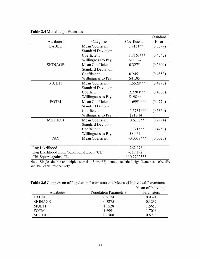
Results of the mixed logit estimation shown in table 2.4 indicate that the
estimated mean coefficients of LABEL, MULTI, and FOTM are positive and
significantly different from zero at the significance level of 0.05, suggesting that these
campaign components are positively valued by participating restaurants. The economic
value of each component is measured as the average WTP for all participating restaurants
which is computed by dividing the coefficient of the component of interest by the
negative of the coefficient of the PAY attribute. For example, the average value of
LABEL in the Certified South Carolina campaign is obtained as , where
is the estimated average scaled effect of LABEL on utility and - is the
estimated marginal utility of money. The results reveal that the FOTM component has an
average WTP across restaurants of $217.14/year. This finding is not surprising given that
restaurants are the most direct beneficiaries of this campaign component. The availability
of multimedia advertising is also highly valued with an average WTP of $198.44/year.
Multimedia advertising sends positive messages about locally grown products to
−θLABEL / θPAY
ˆLABELθ θPAY

19
consumers with the goal of increasing consumer demand that would benefit all campaign
participants. The relatively high WTP by restaurants for this campaign component
supports the current campaign design where the majority of expenses is devoted to
multimedia advertising.8 On the other hand, restaurants usually do not benefit directly
from the point of purchase signage, which explains why the mean coefficient for this
variable is not statistically significant. The significant positive coefficient for METHOD
indicates that restaurants prefer to participate in the Certified South Carolina campaign
by donating annually instead of paying a membership fee.9 Following Holmes and
Adamowicz’s (2003) approach to calculating the compensating variation, our findings
suggest that participating restaurants would be willing to pay an average annual
membership fee of $532.82 or a donation of $613.43 to support a campaign that includes
LABEL, MULTI, and FOTM components.
The standard deviation coefficients for LABEL, MULTI, and FOTM are
significantly different from zero at the 0.05 significance level. These coefficients allow us
to calculate the population shares that place either a positive or negative value on each
attribute. For instance, the distribution of the coefficient of FOTM component has an 8 Another mixed logit model was tested by adding the interaction effect between MULTI and FOTM. Results indicate restaurants’ WTP for having both the FOTM and MULTI components is $374.6 ($98.03+$116.81+$159.82), which is similar to the result of $415.58 ($198.44+$217.14) obtained in the model without the interaction effect. !9 We checked the robustness of the mixed logit results by estimating models excluding, from one group at a time, individuals who responded “unsure” to question 2, 3, 4, and 5 in table 2.3. The sign, magnitude and statistical significance of the mean coefficients were generally consistent across specifications except for the statistical significance of the mean coefficients corresponding to the METHOD attribute. This coefficient was only significant in one of the three alternative specifications. However, the samples used in the alternative specifications were significantly smaller than the original sample size. !
20
estimated mean of 1.70 and an estimated standard deviation of 2.57, suggesting that 75%
of respondents positively value this component within the Certified South Carolina
campaign. Based on this interpretation, 76% of respondents have a positive WTP for the
MULTI component, and 70% of respondents have a positive WTP for the LABEL
component of the Certified South Carolina campaign.
Factors Affecting Campaign Valuation
Table 2.5 reports the mean values of the individual level preference parameters
(!!) estimated using equation (2.9). As shown in the table, the mean values of individual
parameters are very similar to those found for population parameters.10 As in the case of
the population mean WTP, the individual restaurant WTP values for LABEL, SIGNAGE,
MULTI, and FOTM were calculated dividing the estimated individual level parameters
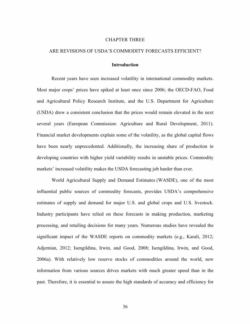
for each component by the negative of the coefficient estimate for PAY. The boxplots
shown in figure 2.2 provide information about the distributional characteristics of these
WTP values. Restaurant managers’ WTP for signage was estimated in a very narrow
range, between $30.5 and $54.3, while the WTP for the FOTM component had the largest
dispersion, between $-313.1 and $687.3. Half of the observations fell into the range of
$28.7 to $213.2 for Labeling, $16.2 to $390.4 for Multimedia Advertising and $32.6 to
$380.1 for the FOTM component. In all cases, more than 75% of restaurants were willing
to pay a positive amount of money for having these campaign components. The numbers
10 This finding is consistent with Train’s (2003) suggestion that the mean of individual-specific parameters derived from a correctly specified model should mirror closely the population parameters. !
21
inside the boxplots are the mean values of individual WTP for each variable; these values
are close to the median of WTP estimates (the vertical line inside the box), suggesting
that distributions are fairly symmetric. Furthermore, the mean values are consistent with
the population mean WTP estimates (reported in a previous section).
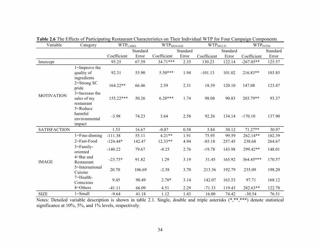
The effects of participating restaurant characteristics on their individual WTP for
campaign components reveal no significant difference in WTP for any component
between big and small restaurants (SIZE) (table 2.6). Restaurants’ WTP for the LABEL
component of the campaign is driven by their motivations and image. The coefficients of
MOTIVATION2 (strong South Carolina pride) and MOTIVATION3 (increase the sales
of my restaurant) are significant in the WTPLABEL equation, suggesting that, ceteris
paribus, these motivations induce restaurants to pay more for the LABEL component of
the campaign. Fast-food restaurants and bars-and-restaurants are willing to pay $124 and
$24 less, respectively, for the LABEL component relative to American cuisine
restaurants.
Motivations also affect restaurants’ WTP for the SIGNAGE component of the
campaign, with restaurants that are trying to improve the quality of their ingredients or
increase sales willing to pay about $6 more than the ones that joined the campaign to
support the South Carolina economy. Fast-food restaurants, fine-dining restaurants and
health-conscious restaurants are willing to pay $12, $4 and $3 more, respectively for the
SIGNAGE component relative to American cuisine restaurants.
Participating restaurants’ WTP for the FOTM component is significantly affected
by their motivations, satisfaction with the campaign and image. For example, restaurants
22
are willing to pay $217 and $204 more for the FOTM campaign if their motivations are to
improve the quality of their ingredients and increase sales, respectively. The coefficient
of the SATISFACTION variable suggests that restaurants are willing to pay $71 more for
having the FOTM component when their satisfaction increases by one unit (on a five
point scale shown in table 2.1). At the same time, fine-dining, family-oriented and bar-
and-restaurant types of restaurants are willing to pay $262, $299, and $364 more,
respectively, for this campaign component compared to American cuisine restaurants,
holding everything else constant. This finding likely reflects differences in the
preferences of restaurants’ clientele 11 and the extent to which different types of
restaurants use locally grown ingredients. Finally, none of the variables affect restaurant
WTP for the MULTI component of the campaign. This result is not surprising given the
very general nature of this component.
The intercepts in the linear models are the WTP values for a large American
cuisine restaurant, which is motivated to participate in the campaign mainly to support
the South Carolina economy, but which is also dissatisfied with the campaign. Two of the
intercepts are statistically different from zero (WTPSIGNAGE and WTPFOTM models). The
estimated intercept value in the WTPFOTM model of -$267 provides another indication of
the importance of this component since the “baseline” restaurant captured in the intercept
has the lowest possible level of satisfaction.
Overall, these findings can help SCDA market the campaign to potential
participants. For example, WTP for both FOTM and SIGNAGE components is
11 For example, Carpio and Isengildina-Massa (2009) showed that consumer preferences for locally grown foods are affected by their age, income, and gender.
23
significantly positively affected by the motivation to increase sales. Our finding showing
that the sales of the participating restaurants were believed to increase by 16% due to
campaign participation can serve as a strong marketing tool for campaign promotion.
Summary and Conclusions
The first objective of this study was to estimate the perceived economic value of
each of the four components of the Certified South Carolina campaign from the
viewpoint of participating restaurants. A choice experiment was conducted as part of a
restaurant manager survey to estimate average WTP for each campaign component using
a mixed logit model. The four existing campaign components were treated as attributes in
mixed logit model estimation, which also included the method of payment and the
amount of payment for the campaign. Findings indicate that three existing campaign
components--Labeling, Multimedia Advertising, and “Fresh on the Menu” have a
significant positive economic value for restaurants participating in the program. The
estimated mean WTP for the components are $117.24, $198.44, and $217.14 per year,
respectively. These estimated WTP values could be used as a guide if a participation fee
is imposed in the future.
The results suggest that restaurants prefer to participate in the Certified South
Carolina campaign by donating annually instead of paying a membership fee.
Nevertheless participating restaurants are willing to pay an average membership fee of
$532.82 annually to support the campaign that includes Labeling, Multimedia
Advertising, and “Fresh on the Menu” components.
24
This study also sheds light on determinants of restaurants’ WTP for the campaign.
We found that restaurants’ image, satisfaction with the campaign, and motivation for
participation significantly affect their WTP for the “Fresh on the Menu”, Signage and
Labeling campaign components. However, restaurants’ size does not affect WTP for any
component. These findings can help the South Carolina Department of Agriculture
marketing the campaign to potential participants.
Currently, the Certified South Carolina campaign is entirely funded by special
appropriations from the state legislature. The economic value of the campaign
demonstrated in this study may help government officials justify the expenditure of
public funds on the operational costs associated with the campaign. Furthermore, our
estimates of the economic value of each of the campaign components allow comparison
of their relative benefits and provides information needed for possible re-allocation of
funds towards the most valued uses. Although our results reflect the view of participating
restaurants only, the framework and survey instruments developed in this study can be
applied to other program participants and beneficiaries (e.g. farmers, farmer’s market
vendors, grocery stores) to draw more general conclusions.
25
References
Adamowicz, W., P. Boxall, M. Williams, and J.J. Louviere. “Stated Preference Approaches for Measuring Passive Use Values: Choice Experiments and Contingent Valuation.” American Journal of Agricultural Economics 80(Feburary 1998):64-75.
Adamowicz, W., J. Swait, R. Boxall, J. Louviere, and M. Williams. “Perception versus Objective Measures of Environmental Quality in Combined Revealed and Stated Prefernce Models of Environmental Valuation.” Journal of Environmental Economics and Management 32(1997):65-84.
Alfnes, F., A. Guttormsen, G. Steine, and K. Kolstad. “Consumers’ Willingness to Pay for the Color of Salmon: a Choice Experiment with Real Economic Incentives.” American Journal of Agricultural Economics 88(November 2006):1050-61.
Bhat, C.R. “Imputing a Continuous Income Variable from Grouped and Missing Income Observations.” Economics Letters 46(December 1994):311-19.
Brick, J.M., D. Martin, P. Warren, and J. Wivagg. “Increased Efforts in RDD Surveys.” 2003 Proceedings of the Section on Survey Research Methods (2003):26-31.
Cameron, A.C., and P.K. Trivedi. Microeconometrics: Methods and Applications. Cambridge, U.K.: Cambridge University Press, 2005.
Carlsson, E, and P. Martinsson. “Do Hypothetical and Actual Marginal Willingness to Pay Differ in Choice Experiments?” Journal of Environmental Economics and Management 41(2001):179-92.
Carpio, C.E., and O. Isengildina-Massa. “Does Government Sponsored Advertising Increase Social Welfare? A Theoretical and Empirical Investigation.” Paper presented at the Agricultural and Applied Economics Association’s 2013 AAEA and CAES Joint Annual Meeting, Washington, DC, August 4-6, 2013.
Carpio, C.E., and O. Isengildina-Massa. “To Fund or Not to Fund: Assessment of the Potential Impact of a Regional Promotion Campaign.” Journal of Agricultural and Resource Economics 35(August 2010):245-60.
Carpio, C.E. and O. Isengildina-Massa. “Consumer Willingness to Pay for Locally Grown Products: the Case of South Carolina.” Agribusiness 25(2009):412-26.
Curtin, R., E. Presser, and E. Singer. “The Effects of Response Rate Changes on the Index of Consumer Sentiment.” Public Opinion Quarterly 64(2000):413-28.
26
Govindasamy, R., B. Schilling, K. Sullivan, C. Turvey, L. Brown, and V.S. Puduri. “Returns to the Jersey Fresh Promotional Program: the Impacts of Promotional Expenditures on Farm Cash Receipts in New Jersey.” Working Paper, Department of Agricultural, Food and Resource Economics and the Food Policy Institute, Rutgers, The State University of New Jersey, 2003.
Hamilton, M.B. “Online Survey Response Rates and Times: Background and Guidance for Industry.” Ipathia, Inc./SuperSurvey (2003). Internet site: http://www.supersurvey.com/papers/supersurvey_white_paper_response_rates.pdf (Accessed June 1, 2013)
Hanemann, M., J. Loomis, and B. Kanninen. “Statistical Efficiency of Double-Bounded Dichotomous Choice Contingent Valuation.” American Journal of Agricultural Economics 73(November 1991):1255-63.
Hasing, T., C.E. Carpio, D.B. Willis, O. Sydorovych, and M. Marra. “The Effect of Label Information on U.S. Farmers’ Herbicide Choices.” Agricultural and Resource Economics Review 41(August 2012):200-14.
Hensher, D., N. Shore, and K. Train. “Households Willingness to Pay for Water Service Attributes.” Environmental and Resource Economics 32(2005):509-31.
Holbrook, A., J. Krosnick, A. Pfent. “The Causes and Consequences of Response Rates in Surveys by the News Media and Government Contractor Survey Research Firms.” Advances in telephone survey methodology. J.M. Lepkowski, C. Tucker, J.M. Brick, E.D. de Leeuw, L. Japec, P.J. Lavrakas, M.W. Link, and R.L. Sangster, eds. New York: Wiley, 2007.
Holmes, T. P. and W. L. Adamowicz. “Attribute-based methods.” A Primer on Nonmarket Valuation. P.A. Champ, K.J. Boyle, and T.C. Brown, eds. Dordrecht, Netherlands: Springer, 2003.
Keeter, S., C. Kennedy, M. Dimock, J. Best, P. Craighill. “Gauging the Impact of Growing Nonresponse on Estimates from a National RDD Telephone Survey.” Public Opinion Quarterly 70(2006):759-79.
Keeter, S., C. Miller, A. Kohut, R. Groves, and S. Presser. “Consequences of Reducing Nonresponse in a Large National Telephone Survey.” Public Opinion Quarterly 64(2000): 125-48.
List, J.A. and J.F. Shogren. “Calibration of the Difference Between Actual and Hypothetical Valuations in a Field Experiment.” Journal of Economic Behavior and Organization 37(1998):193-205.
27
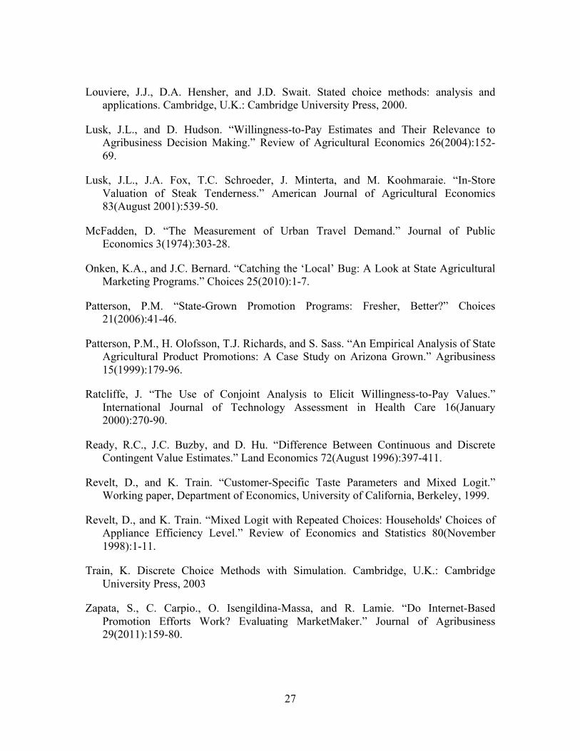
Louviere, J.J., D.A. Hensher, and J.D. Swait. Stated choice methods: analysis and applications. Cambridge, U.K.: Cambridge University Press, 2000.
Lusk, J.L., and D. Hudson. “Willingness-to-Pay Estimates and Their Relevance to Agribusiness Decision Making.” Review of Agricultural Economics 26(2004):152-69.
Lusk, J.L., J.A. Fox, T.C. Schroeder, J. Minterta, and M. Koohmaraie. “In-Store Valuation of Steak Tenderness.” American Journal of Agricultural Economics 83(August 2001):539-50.
McFadden, D. “The Measurement of Urban Travel Demand.” Journal of Public Economics 3(1974):303-28.
Onken, K.A., and J.C. Bernard. “Catching the ‘Local’ Bug: A Look at State Agricultural Marketing Programs.” Choices 25(2010):1-7.
Patterson, P.M. “State-Grown Promotion Programs: Fresher, Better?” Choices 21(2006):41-46.
Patterson, P.M., H. Olofsson, T.J. Richards, and S. Sass. “An Empirical Analysis of State Agricultural Product Promotions: A Case Study on Arizona Grown.” Agribusiness 15(1999):179-96.
Ratcliffe, J. “The Use of Conjoint Analysis to Elicit Willingness-to-Pay Values.” International Journal of Technology Assessment in Health Care 16(January 2000):270-90.
Ready, R.C., J.C. Buzby, and D. Hu. “Difference Between Continuous and Discrete Contingent Value Estimates.” Land Economics 72(August 1996):397-411.
Revelt, D., and K. Train. “Customer-Specific Taste Parameters and Mixed Logit.” Working paper, Department of Economics, University of California, Berkeley, 1999.
Revelt, D., and K. Train. “Mixed Logit with Repeated Choices: Households' Choices of Appliance Efficiency Level.” Review of Economics and Statistics 80(November 1998):1-11.
Train, K. Discrete Choice Methods with Simulation. Cambridge, U.K.: Cambridge University Press, 2003
Zapata, S., C. Carpio., O. Isengildina-Massa, and R. Lamie. “Do Internet-Based Promotion Efforts Work? Evaluating MarketMaker.” Journal of Agribusiness 29(2011):159-80.
28
Table 2.1 Description of Variables Included in the OLS Method
Variable Description Category Category
Proportion MOTIVATION Which of the
following reasons was the most important motivation for you to join the Certified South Carolina Campaign “Fresh on the Menu” Program?
1=Improve the quality of ingredients since SC produces the better quality products
20.69%
2=Strong SC pride 15.52% 3=Increase the sales of my restaurant by attracting customers interested in SC products
27.59%
4=Support SC economy 32.75% 5=Reduce harmful environmental impact (carbon footprint)
3.45%
SATISFACTION How would you rate your overall satisfaction with the campaign?
0=Very dissatisfied 15.52% 1=Dissatisfied 12.07% 2=Neutral 29.31% 3=Satisfied 18.97% 4=Very satisfied 24.14%
IMAGE How would you best describe the focus/image of your restaurant?
1=Fine-dining 30.36% 2=Fast-Food 1.79% 3=Family-oriented 10.71% 4=Bar and Restaurant 5.36% 5=International Cuisine 3.57% 6=American Cuisine 21.43% 7=Health-Conscious 7.14% 8=Other, please specify 19.64%
SIZE Please describe the size of your restaurant business in 2009 in terms of total annual sales.
1=$1,000-$9,999 3.64% 2=$10,000-$49,999 0.00% 3=$50,000-$99,999 5.45% 4=$100,000-$249,000 16.36% 5=$250,000-$499,000 23.64% 6=$500,000 and over 50.91%
Note: The response rate varies across questions with the minimum sample size of 55.
29
Table 2.2 Summary Statistics Describing the Characteristics of Restaurants Participating in the Certified South Carolina Campaign “Fresh on the Menu” Program
Question Category Category Proportion Mean Standard
Deviation
Which of the following reasons was the most important motivation for you to join the Certified South Carolina campaign“ Fresh on the Menu” Program?
1=Improve the quality of ingredients since South Carolina produces the better quality products
20.97%
2=Strong South Carolina pride
14.52%
3=Increase the sales of my restaurant by attracting customers interested in South Carolina products
25.81%
4=Support South Carolina economy
35.48%
5=Reduce harmful environmental impact (carbon footprint)
3.23%
How did you learn about the campaign?
1=Magazines 3.20% 2=Direct Mailing 9.50% 3=Food Service Food Show
14.30%
4=Direct contact from the SCDA
27.00%
5=Fresh on the Menu website
15.90%
6=Other Restaurants 6.40% 7=Other 23.80%
How would you best describe the focus/image of your restaurant?
Fine-dining 30.00%
Fast-Food 1.67% Family-oriented 11.67% Bar and Restaurant 5.00% International Cuisine 3.33% American Cuisine 23.33% Health-Conscious 6.67% Other 18.33%
30
Table 2.2 (Continued)
Question Category Category Proportion Mean Standard
Deviation
Please describe the size of your restaurant business in 2009 in terms of total annual sales
$1,000-$9,999 3.39%
$385,080 $22,860
$10,000-$49,999 $50,000-$99,999 5.08% $100,000-$249,000 15.25% $250,000-$499,000 23.73% $500,000 and over 52.54%
How would you best describe the ownership of your restaurant?
Locally Owned 93.55%
Franchise 6.45%
Age
18-20 years
47.03 years 1.47 years
21-30 years 5.36% 31-40 years 19.64% 41-50 years 33.93% 51-60 years 28.57% 61-69 years 10.71% 70 years or more 1.79%
Gender Male 62.96% Female 37.04%
Highest Level of Education
High School Diploma (including GED)
23.21%
College Degree 53.57% Post-Graduate or Professional Degree 23.21%
Notes: The sample size for this table is different from the sample size in Table 2.1 and the minimum sample size is 54. Since responses were given in the form of intervals, the mean and standard deviation were calculated by applying the parametric approach following Bhat (1994) and Zapata et al. (2011).
31
Table 2.3 Summary Statistics Describing the Perceived Effects of Restaurant Participation in the Certified South Carolina Campaign “Fresh on the Menu” Program
Question Category Category
Proportion Parametric
Meanc Standard Deviation
1. Please describe the costs of your participation in the Certified South Carolina Campaign “Fresh on the Menu” Program in the last year.
$0-$49 55.74%
$129.42 $21.49
$50-$99 13.11% $100-$249 11.48% $250-$499 11.48% $500 and over
8.20%
2. How do you think the campaign affected your costs of purchasing ingredients and preparation in the last year?a
Increase 36.50% Decrease 11.10% Unsure 14.30% No change 38.10%
2-1. What percentage increase in the costs of purchasing ingredients and food preparation?d
0-10% 36.84%
17.97% 4.31% 11-20% 42.11% 21-30% 10.53% 41-50% 5.26% 81-90% 5.26%
2-2. What percentage decrease in the costs of purchasing ingredients and food preparation?e
0-10% 71.43%
9.56% 2.88% 11-20% 14.29% 21-30% 14.29%
3. How do you think the campaign affected your total sales during the last year?a
Increase 38.10% Decrease 0.00% Unsure 38.10% No change 23.80%
3-1. What percentage increase in total sales?d
0-10% 43.48%
16.19% 3.11%
11-20% 34.78% 21-30% 8.7% 31-40% 4.35% 41-50% 4.35% 61-70% 4.35%
4. How do you think the campaign affected the number of clientele visiting your restaurant in the last year?a
Increase 31.70% Decrease 0.00% Unsure 41.30% No change 27.00%
4-1. What percentage increase in the number of clientele?d
0-10% 36.84%
16.41% 2.92% 11-20% 36.84% 21-30% 15.79% 31-40% 5.26% 51-60% 5.26%
32
Table 2.3 (Continued)
a Sample size is 63; b Sample size is 61; c Since responses were given in the form of intervals, the parametric mean and standard deviation were calculated by applying the parametric approach following Bhat (1994) and Zapata et al. (2011). d Questions only asked to individuals who selected “increase” in question 2, 3, 4 and 5, respectively; e Questions are responded to people who select “decrease” in question 2 and 5, respectively;
Question Category Category
Proportion Parametric
Meanc Standard Deviation
5. How do you think the campaign affected the profitability of your restaurant in the last year?b
Increase 22.95% Decrease 3.28% Unsure 34.43% No change 39.34%
5-1. What percentage increase in profitability?d
0-10% 66.67%
15.2% 4.94% 11-20% 8.33% 21-30% 8.33% 41-50% 8.33% 51-60% 8.33%
5-2. What percentage decrease in profitability?e 0-10% 100% 5% 0%
33
Table 2.4 Mixed Logit Estimates
Attributes Categories Coefficient Standard
Error LABEL Mean Coefficient 0.9174** (0.3899)
Standard Deviation Coefficient 1.7167*** (0.4742)
Willingness to Pay $117.24 SIGNAGE Mean Coefficient 0.3275 (0.2609)
Standard Deviation Coefficient 0.2451 (0.4853)
Willingness to Pay $41.85 MULTI Mean Coefficient 1.5528*** (0.4295)
Standard Deviation Coefficient 2.2200*** (0.4800)
Willingness to Pay $198.44 FOTM Mean Coefficient 1.6991*** (0.4774)
Standard Deviation Coefficient 2.5734*** (0.5360)
Willingness to Pay $217.14 METHOD Mean Coefficient 0.6308** (0.2994)
Standard Deviation Coefficient 0.9213** (0.4258)
Willingness to Pay $80.61 PAY Mean Coefficient -0.0078*** (0.0023)
Log Likelihood -262.0784 Log Likelihood from Conditional Logit (CL) -317.192 Chi-Square against CL 110.2272***
Note: Single, double and triple asterisks (*,**,***) denote statistical significance at 10%, 5%, and 1% levels, respectively. Table 2.5 Comparison of Population Parameters and Means of Individual Parameters
Attributes Population Parameters Mean of Individual
parameters LABEL 0.9174 0.9391 SIGNAGE 0.3275 0.3297 MULTI 1.5528 1.5658 FOTM 1.6991 1.7016 METHOD 0.6308 0.6228
!
! 34
Table 2.6 The Effects of Participating Restaurant Characteristics on Their Individual WTP for Four Campaign Components Variable Category WTPLABEL WTPSIGNAGE WTPMULTI WTPFOTM
Coefficient
Standard Error
Coefficient
Standard Error
Coefficient
Standard Error
Coefficient
Standard Error
Intercept 95.25 67.59 34.71*** 2.35 130.23 122.14 -267.05** 125.57
MOTIVATION
1=Improve the quality of ingredients
92.31 55.90 5.50*** 1.94 -101.13 101.02 216.83** 103.85
2=Strong SC pride 164.22** 66.46 2.59 2.31 18.39 120.10 147.08 123.47
3=Increase the sales of my restaurant
155.22*** 50.26 6.28*** 1.74 98.08 90.83 203.79** 93.37
5=Reduce harmful environmental impact
-3.98 74.23 3.64 2.58 92.26 134.14 -170.10 137.90
SATISFACTION 1.53 16.67 -0.07 0.58 3.84 30.12 71.27** 30.97
IMAGE
1=Fine-dinning -111.38 55.11 4.21** 1.91 75.95 99.59 262.14** 102.39 2=Fast-Food -124.44* 142.47 12.33** 4.94 -85.18 257.45 238.68 264.67 3=Family-oriented -140.22 79.67 -0.25 2.76 -19.78 143.98 299.42** 148.01
4=Bar and Restaurant -23.75* 91.82 1.29 3.19 31.45 165.92 364.45*** 170.57
5=International Cuisine 20.70 106.69 -2.58 3.70 213.36 192.79 235.09 198.20
7=Health-Conscious 9.45 90.49 2.70* 3.14 142.07 163.53 97.71 168.12
8=Others -41.11 66.09 4.51 2.29 -71.33 119.43 282.63** 122.78 SIZE 1=Small -9.64 41.18 1.12 1.43 16.00 74.42 -30.54 76.51
Notes: Detailed variable description is shown in table 2.1. Single, double and triple asterisks (*,**,***) denote statistical significance at 10%, 5%, and 1% levels, respectively.
!
! 35
Scenario 1
Campaign A Components/Costs Campaign B
Not included Labeling Included
Not included Point of Purchase
Signage Not included
Not included Multimedia Advertising Not included
Included “Fresh on the Menu” Not included Annual membership fee
of $20 Funding Annual donation of
$100
If you were given three choices: Campaign A, Campaign B, or not having a campaign at all, which would you choose?
___Campaign A ___Campaign B ___Not campaign at all Figure 2.1 Example of One of the Scenarios from the Restaurant Survey
Figure 2.2 Box Plot of WTP for LABEL, SIGNAGE, MULTI, and FOTM
36
CHAPTER THREE
ARE REVISIONS OF USDA’S COMMODITY FORECASTS EFFICIENT?
Introduction
Recent years have seen increased volatility in international commodity markets.
Most major crops’ prices have spiked at least once since 2006; the OECD-FAO, Food
and Agricultural Policy Research Institute, and the U.S. Department for Agriculture
(USDA) drew a consistent conclusion that the prices would remain elevated in the next
several years (European Commission: Agriculture and Rural Development, 2011).
Financial market developments explain some of the volatility, as the global capital flows
have been nearly unprecedented. Additionally, the increasing share of production in
developing countries with higher yield variability results in unstable prices. Commodity
markets’ increased volatility makes the USDA forecasting job harder than ever.
World Agricultural Supply and Demand Estimates (WASDE), one of the most
influential public sources of commodity forecasts, provides USDA’s comprehensive
estimates of supply and demand for major U.S. and global crops and U.S. livestock.
Industry participants have relied on these forecasts in making production, marketing
processing, and retailing decisions for many years. Numerous studies have revealed the
significant impact of the WASDE reports on commodity markets (e.g., Karali, 2012;
Adjemian, 2012; Isengildina, Irwin, and Good, 2008; Isengildina, Irwin, and Good,
2006a). With relatively low reserve stocks of commodities around the world, new
information from various sources drives markets with much greater speed than in the
past. Therefore, it is essential to assure the high standards of accuracy and efficiency for

37
WASDE reports. However, concerns have surfaced about the reliability of USDA
forecasts. In December 2011, the Wall Street Journal reported that over the previous two
years, USDA’s monthly forecasts of how much farmers will produce has been, “off the
mark to a greater degree than any other two consecutive years in the last 15 [years].”
Several recent studies examined the accuracy and efficiency of WASDE
forecasts. Sanders and Manfredo (2002) found that beef and pork production forecasts
inefficiently incorporated available information and showed the existence of positive
serial correlation in errors of beef and poultry production forecasts. Sanders and
Manfredo (2003) examined the WASDE price forecasts for cattle, hogs, and broilers and
found overestimation in broiler price forecasts and inefficiency in a number of livestock
price forecasts due to repeated forecast errors. Isengildina, Irwin, and Good (2004)
evaluated corn and soybean price forecasts using interval accuracy tests and rejected
forecast accuracy at the 95% level for both commodities. Botto et al. (2006) analyzed
forecast accuracy of all categories for corn and soybeans, and they found inefficiency in
soybean ending stocks and price forecasts. More recently, Isengildina-Massa,
MacDonald, and Xie (2012) incorporated a variety of tests to evaluate the forecast
performance of WASDE cotton forecasts for the U.S. and China. They discovered that
the most pervasive rejection of efficiency across variables and countries occurred in tests
of revision efficiency. Lewis and Manfredo (2012) concluded that the sugar production
and consumption forecasts are less problematic as inefficiency was only found in a few
cases. Although all of these studies demonstrated the inefficiency of WASDE across
38
different commodities, none of them provided guidance on how to improve forecast
accuracy.
Isengildina, Irwin, and Good (2006b) focused on forecast revision efficiency,
which had been largely overlooked in the previous studies. The forecast revisions process
is important to reveal how forecasts change across the forecasting cycle and how
analyzing forecast revisions allows the detection of inefficiency due to systematic
under/over-adjustments in forecasts. Isengildina, Irwin, and Good (2006b) found the
existence of revision inefficiency in WASDE corn and soybean production forecasts and
suggested a procedure based on Nordhaus’s (1987) approach to successfully correct for
inefficiency in revisions. However, their procedure was rather simplistic and the results
were limited to corn and soybean production forecasts.
The goal of this study was to expand Isengildina, Irwin, and Good’s work to
include 1) evaluation of monthly revisions efficiency of all supply, demand, and price
categories for U.S. corn, soybean, wheat, and cotton forecasts, published in the monthly
WASDE reports between 1984/85 through 2011/12; and 2) development of a new
inefficiency correction procedure that takes into account adjusting for outliers,
controlling for the impact of other variables on inefficiency, and considering structural
changes.
Data
This study focused on monthly WASDE U.S. corn, soybean, wheat, and cotton
forecasts from 1984/85 through 2011/12. Typically, WASDE reports were released
between the 9th and 12th of each month. Prior to May 1994, WASDE reports were
39
published at 3:00 p.m. in the Eastern Time Zone of the U.S., but the report release time
was changed to 8:30 a.m. between May 1994 and December 2012.
Vogel and Bange (1999) describe that forecasts of U.S. crop production are
independently prepared by the National Agricultural Statistics Services, while supply
(other than production), demand, and price forecasts are developed jointly by several
USDA agencies. The World Agricultural Outlook Board coordinates the high-security
interagency process by chairing an Interagency Commodity Estimates Committee (ICEC)
of leaders responsible for each commodity. Joint forecast preparation enables USDA
analysts to incorporate all available resources and assures that the estimates are consistent
across all USDA publications.
WASDE supply and demand forecasts apply a full balance-sheet approach for
each commodity, which means that the total supply must equal the demand. The total
supply of a crop is comprised of beginning stocks, imports, and production. The demand
side of the balance sheet includes domestic use, exports, and ending stocks. Domestic use
is further subdivided into feed and residual, and food, seed and industrial for corn;
crushings, seed, and residual for soybeans; and feed and residual, food, and seed for
wheat.12 The ending stocks for a marketing year t become the beginning stocks for year
t+1. While price forecasts are published in interval form, other categories’ forecasts are
point estimates. To overcome this inconsistency and keep the analysis consistent across
12 More detail on the balance-sheet nature of WASDE forecasts and the forecast generation procedure is given in Vogel and Bange (1999).
40
all categories, midpoints of the price forecast intervals are considered in our analysis.13
WASDE are forecasted on a marketing year basis, which spans from September
to August for corn and soybeans, from June to May for wheat, and from August to July
for cotton. The first forecasts for all crops of each marketing year are published in May
preceding the marketing year. Beginning stocks and production forecasts are typically
finalized after the harvest time of each crop, by October for wheat and January for corn,
soybeans, and cotton14. Estimates for other forecast categories are generally finalized by
November after the marketing year. Therefore, production and beginning stocks’
forecasting cycles are 9 months for corn, soybeans, and cotton, and 6 months for wheat.
The forecasting cycles are 19 months for all crops’ other categories. Figure 3.1 illustrates
the 2011/12 marketing year and the relative WASDE forecasting cycles for commodities
included in this study.
WASDE forecasts are considered fixed-event forecasts because the series of
forecasts are related to the same terminal event ytJ, where J is the release month of the
final estimate for a marketing year t, and t=1(1984/85),…,28(2011/12). J=9 for
production and beginning stocks forecasts for corn, soybeans, and cotton, and J=6 for
those two categories for wheat; J=19 for all crops’ other categories. The terminal event 13 USDA was prohibited from publishing forecasts of cotton prices from 1929 to 2008, but USDA’s ICEC for cotton calculated unpublished price forecasts each month as point estimates. Since 2008, cotton price forecasts have been published in interval form. Also, for all four commodities, the price forecasts typically converge to point estimates by April of the marketing year. 14 WASDE frequently published the revised estimate of final soybean production in October after the marketing year. The final forecasts of the cotton production were commonly revised in April and May of the subsequent year. Also, WASDE sometimes revised the final forecasts of the wheat beginning stocks and production in January and October, respectively. Because these additional revisions were somewhat sporadic in nature, they are not included in our analysis.
41
for supply and demand categories describes a total volume, while the terminal event for
the price category represents a marketing year’s average value for price. The forecasted
value published in month j is denoted as ytj, where j=1,…,J. Therefore, each subsequent
forecast is an update of the previous forecast describing the same terminal event. Based
on the definition of forecasting cycles from the data section, WASDE generates 18
updates/revisions for each U.S. category except for production and beginning stocks (8
updates for corn, soybeans, and cotton, and 5 updates for wheat).
Methods
Forecast Revision Efficiency
The tests of efficiency in forecast revisions were originally developed by
Nordhaus in 1987 and have since been used extensively in the macroeconomic literature
(e.g., Clements, 1997; Harvey et al., 2001; Patton and Timmermann, 2010; Dovern and
Weisser, 2011) and less frequently in agricultural forecasting (Isengildina, Irwin, and
Good, 2006b; Lewis and Manfredo, 2012). Within the Nordhaus framework, if fixed
event forecasts are weak-form efficient, their revisions should follow a random walk.
In this study, forecast revisions were defined as the difference between two
adjacent forecasts. In order to standardize for increasing crop size over time, forecast
revisions were examined in log percentage form:
(3.1) , 28...,,1;,...,2ln*100 1 ==⎟⎟⎠
⎞⎜⎜⎝
⎛= − tJj
yyr jt
jtj
t
42
where is a revision of a forecast for marketing year t released in month j-1. Figure 3.2
illustrates the layout of the fixed event forecasting cycle and the corresponding forecast
revisions process using corn production as an example.
Following Isengildina, Irwin, and Good (2006b), efficiency of WASDE forecast
revisions was examined as:
(3.2) j = 2, …, J; t =1,…,28.
Thus, for j = 3, λ represents the slope coefficient for all July revisions made from 1984/85
to 2011/12 regressed against the June revisions (j – 1 = 2) for the same years. The null
hypothesis for efficiency in forecast revisions was λ = 0. If λ > 0, the forecasts are
considered “smoothed”, as they are partially based on the previous revision. If λ < 0, the
forecasts are called “jumpy”, as they tend to partially offset the previous revision. The
test of Ho that λ = 0 required at least 3 rolling-event forecasts to generate a revision and a
lagged revision which limited our ability to analyze revision efficiency in the first 2
forecasts of each marketing year. Therefore, month 3 was the first month analyzed.
Equation (3.2) was estimated using the method of Ordinary Least Squares (OLS) for each
forecast category for each crop.
Correction for Revision Inefficiency
The Basic Correction Procedure
The basic procedure for correcting revision inefficiency was described in Isengildina,
Irwin and Good (2006b). Since in equation (3.2), revision inefficiency in one month
(rejection of Ho that λ = 0), signals a failure in the previous month to appropriately
jtr
jt
jt
jt rr ελ += −1

43
incorporate all new information, an alternative measure for inefficiency correction that
provides an adjustment parameter γ for a pending, as opposed to a past revision was used:
(3.3) j = 1, …, J - 1; t =1,…,28,
where etj is the forecast error of a forecast for marketing year t released in month j, and
rtj+1 is the forecast revision for the same marketing year t released in the next month.
Consistently with forecast revisions, forecast errors were calculated in log percentage
form:
(3.4) .
Equation (3.3) was based on Nordhaus’ (1987) derivation that the forecast error at
time j should be fully corrected (on average) by the following revision(s), thus, if
revisions are efficient, γ=1. According to Isengildina, Irwin and Good (2006b), out-of-
sample correction of revision inefficiency should proceed along the following steps: 1)
estimate γ coefficients using equation (3.3) and the data in the estimation subsample, 2)
multiply published revisions by γ coefficients to derive efficient revisions,15 and 3)
calculate adjusted forecasts by adding efficient revisions to the previous months’
forecasts.
For example, if was estimated using 1984/85-1993/94 May forecast errors (etj,
t=1,…,10 and j=1) and June forecast revisions (rtj+1, t=1,…,10, and j=1), the adjusted
15 We follow a more conservative approach by adjusting revisions and forecasts only when the estimated γ coefficients are significant at a significance level of 0.05. Results of adjusting all revisions and forecasts regardless of the significance of the estimated γ coefficients are available upon request.
etj =α + γ rt
j+1 + ε tj
28...,,1;1,...,1ln*100 =−=⎟⎟⎠
⎞⎜⎜⎝
⎛= tJj
yye jt
Jtj
t
γ
44
revision for June 1994/95 (!!!!!, t=11 and j=1) was the product of and !!!! . Because the
forecast errors and revisions were defined in logarithm terms in this study, the June
1994/95 adjusted forecasts were calculated as !!!! = !!!! ∗ !(!!!! !"").
While Isengildina, Irwin and Good (2006b) demonstrated that such revision
inefficiency correction improved the accuracy of corn and soybean production forecasts
in their 1980/81-2004/05 validation subsample, their procedure may have suffered from
several potential limitations. First, an OLS regression was used to estimate in equation
(3.3), so the estimates might be influenced by the presence of outliers. Second, other
variables might affect smoothing. For example, Isengildina, Irwin and Good (2013)
argued that “big crops get bigger and small crops get smaller,” which suggests that
forecast size and direction should be considered in adjusting forecasts for smoothing.
Third, stability of revision inefficiency over time would have implications on how well
the correction procedure would improve accuracy: if the inefficiency is unstable, the
adjustment procedure would perform poorly and modifications must be made. Our
approach to incorporating these additional factors in the revision inefficiency correction
procedure is described in the following sections.
Outlier Detection
Rousseeuw and Leroy (2005) argued that regression outliers (either in the
dependent or independent variable) pose a serious threat to the interpretation of results
from a standard least squares analysis. They suggested two approaches to identify and
deal with outliers, including regression diagnostics and robust regression. Diagnostics
include statistics, such as the Hat Matrix (Hoaglin and Welsch, 1978) and the Cook’s D
γ
γ

45
(Cook, 1977), computed from the data so as to discover influential points. On the other
hand, robust regression methods have been developed to find estimators that are not
strongly affected by outliers as they assign less weight to “abnormal” values.
In this study, the existence of outliers in estimating equation (3.3) using the OLS
method was detected by Cook’s D, which is a measure that combines the information on
leverage (a measure of how far an independent variable deviates from its mean) and
residual (the difference between the predicted value and the observed value) of the
observation. A data point is considered an outlier if the corresponding Cook’s D value is
bigger than 4/n (Rawlings, Pantula, and Dickey, 1998), where n is the sample size. To
handle outliers, robust regression was used for estimating the γ coefficients in equation
(3.3) because outliers could not be simply removed or corrected. In this study, a detected
outlier represents a sudden change in revision inefficiency level. Robust regression has
been applied in numerous fields, such as policy, finance, and economics, etc. (e.g.
Alesina and Perotti, 1996; Preminger et. al., 2007; Finger, 2010). However, we are not
aware of any previous studies that applied robust regression to agricultural forecasts.
Maximum likelihood-type estimation (M-estimation) by Huber (1964) and multiple M-
estimation (MM-estimation) methods by Yohai (1987) were considered in this study,
since they were the most commonly used robust estimations and both methods were
accessible in statistical software R.
Forecast Size and Direction
The influence of forecast size and direction on revision inefficiency should also
be considered in the adjustment procedure because forecast size and direction could be
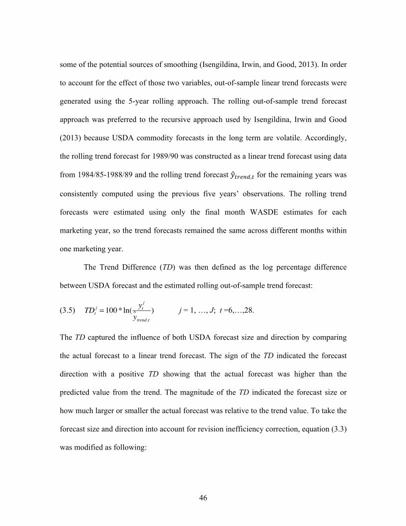
46
some of the potential sources of smoothing (Isengildina, Irwin, and Good, 2013). In order
to account for the effect of those two variables, out-of-sample linear trend forecasts were
generated using the 5-year rolling approach. The rolling out-of-sample trend forecast
approach was preferred to the recursive approach used by Isengildina, Irwin and Good
(2013) because USDA commodity forecasts in the long term are volatile. Accordingly,
the rolling trend forecast for 1989/90 was constructed as a linear trend forecast using data
from 1984/85-1988/89 and the rolling trend forecast !!"#$%,! for the remaining years was
consistently computed using the previous five years’ observations. The rolling trend
forecasts were estimated using only the final month WASDE estimates for each
marketing year, so the trend forecasts remained the same across different months within
one marketing year.
The Trend Difference (TD) was then defined as the log percentage difference
between USDA forecast and the estimated rolling out-of-sample trend forecast:
(3.5) j = 1, …, J; t =6,…,28.
The TD captured the influence of both USDA forecast size and direction by comparing
the actual forecast to a linear trend forecast. The sign of the TD indicated the forecast
direction with a positive TD showing that the actual forecast was higher than the
predicted value from the trend. The magnitude of the TD indicated the forecast size or
how much larger or smaller the actual forecast was relative to the trend value. To take the
forecast size and direction into account for revision inefficiency correction, equation (3.3)
was modified as following:
TDt
j = 100*ln( ytj
y! trend ,t)
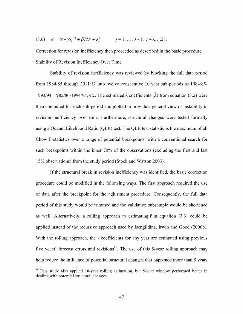
47
(3.6) j = 1, …, J - 1; t =6,…,28.
Correction for revision inefficiency then proceeded as described in the basic procedure.
Stability of Revision Inefficiency Over Time
Stability of revision inefficiency was reviewed by blocking the full data period
from 1984/85 through 2011/12 into twelve consecutive 10 year sub-periods as 1984/85-
1993/94, 1985/86-1994/95, etc. The estimated λ coefficients (!) from equation (3.2) were
then computed for each sub-period and plotted to provide a general view of instability in
revision inefficiency over time. Furthermore, structural changes were tested formally
using a Quandt Likelihood Ratio (QLR) test. The QLR test statistic is the maximum of all
Chow F-statistics over a range of potential breakpoints, with a conventional search for
such breakpoints within the inner 70% of the observations (excluding the first and last
15% observations) from the study period (Stock and Watson 2003).
If the structural break in revision inefficiency was identified, the basic correction
procedure could be modified in the following ways. The first approach required the use
of data after the breakpoint for the adjustment procedure. Consequently, the full data
period of this study would be trimmed and the validation subsample would be shortened
as well. Alternatively, a rolling approach to estimating ! in equation (3.3) could be
applied instead of the recursive approach used by Isengildina, Irwin and Good (2006b).
With the rolling approach, the γ coefficients for any year are estimated using previous
five years’ forecast errors and revisions16. The use of this 5-year rolling approach may
help reduce the influence of potential structural changes that happened more than 5 years 16 This study also applied 10-year rolling estimation, but 5-year window performed better in dealing with potential structural changes.
etj =α + γ rt
j+1 + βTDtj + ε t
j
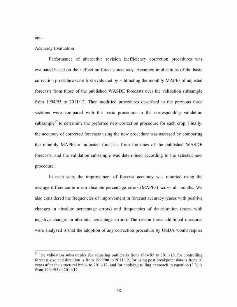
48
ago.
Accuracy Evaluation
Performance of alternative revision inefficiency correction procedures was
evaluated based on their effect on forecast accuracy. Accuracy implications of the basic
correction procedure were first evaluated by subtracting the monthly MAPEs of adjusted
forecasts from those of the published WASDE forecasts over the validation subsample
from 1994/95 to 2011/12. Then modified procedures described in the previous three
sections were compared with the basic procedure in the corresponding validation
subsample17 to determine the preferred new correction procedure for each crop. Finally,
the accuracy of corrected forecasts using the new procedure was assessed by comparing
the monthly MAPEs of adjusted forecasts from the ones of the published WASDE
forecasts, and the validation subsample was determined according to the selected new
procedure.
In each step, the improvement of forecast accuracy was reported using the
average difference in mean absolute percentage errors (MAPEs) across all months. We
also considered the frequencies of improvement in forecast accuracy (cases with positive
changes in absolute percentage errors) and frequencies of deterioration (cases with
negative changes in absolute percentage errors). The reason these additional measures
were analyzed is that the adoption of any correction procedure by USDA would require
17 The validation sub-samples for adjusting outliers is from 1994/95 to 2011/12, for controlling forecast size and direction is from 1999/00 to 2011/12, for using post breakpoint data is from 10 years after the structural break to 2011/12, and for applying rolling approach in equation (3.3) is from 1994/95 to 2011/12.
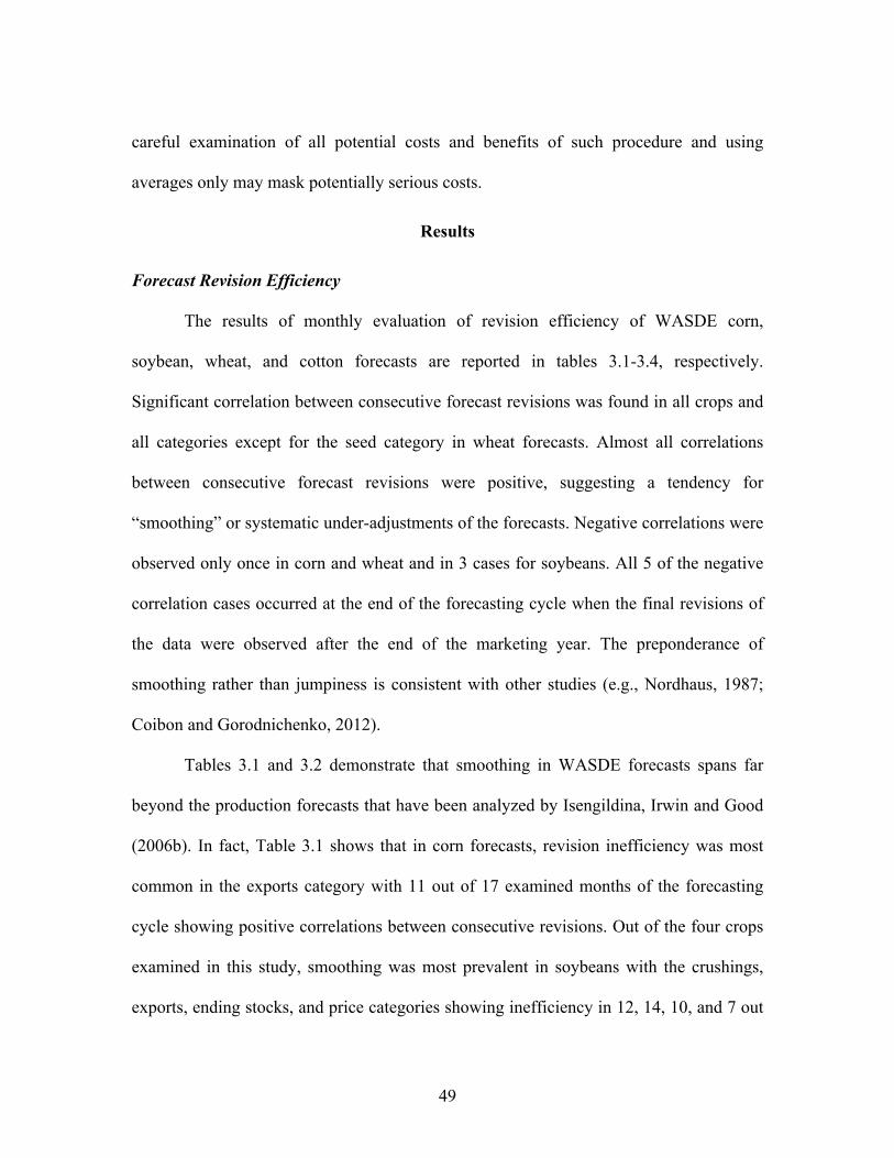
49
careful examination of all potential costs and benefits of such procedure and using
averages only may mask potentially serious costs.
Results
Forecast Revision Efficiency
The results of monthly evaluation of revision efficiency of WASDE corn,
soybean, wheat, and cotton forecasts are reported in tables 3.1-3.4, respectively.
Significant correlation between consecutive forecast revisions was found in all crops and
all categories except for the seed category in wheat forecasts. Almost all correlations
between consecutive forecast revisions were positive, suggesting a tendency for
“smoothing” or systematic under-adjustments of the forecasts. Negative correlations were
observed only once in corn and wheat and in 3 cases for soybeans. All 5 of the negative
correlation cases occurred at the end of the forecasting cycle when the final revisions of
the data were observed after the end of the marketing year. The preponderance of
smoothing rather than jumpiness is consistent with other studies (e.g., Nordhaus, 1987;
Coibon and Gorodnichenko, 2012).
Tables 3.1 and 3.2 demonstrate that smoothing in WASDE forecasts spans far
beyond the production forecasts that have been analyzed by Isengildina, Irwin and Good
(2006b). In fact, Table 3.1 shows that in corn forecasts, revision inefficiency was most
common in the exports category with 11 out of 17 examined months of the forecasting
cycle showing positive correlations between consecutive revisions. Out of the four crops
examined in this study, smoothing was most prevalent in soybeans with the crushings,
exports, ending stocks, and price categories showing inefficiency in 12, 14, 10, and 7 out
50
of 17 months, respectively. Smoothing was the least common in wheat with the most
affected categories of exports and prices exhibiting positive correlations in 5 and 6 out of
17 months, respectively. In cotton, smoothing was most frequent in production, domestic
use, exports and ending stocks forecasts. Prevalence of smoothing seemed to be most
common between November and January for corn, in August and from November to
September for soybeans, from September to December for wheat, and from January to
April for cotton.
Smoothing in production forecasts has been a focus of previous studies because it
is commonly observed by forecast users and could affect other forecasts due to the
balance-sheet nature of WASDE reports. We did find some evidence of the influence of
smoothing in production on other categories as smoothing in November corn production
forecast revisions was accompanied by smoothing in exports, ending stocks, and price
forecast revisions, and smoothing in August and November soybean production forecast
revisions was accompanied by smoothing in almost all other categories. We found similar
patterns in July forecasts for wheat and in July and January forecasts for cotton. Our
findings of smoothing in corn and soybean November production revisions are consistent
with the findings in Isengildina, Irwin, and Good (2006b) in both the magnitude and
significance level. The estimated coefficients can be interpreted as point elasticities and
indicate, for example, that on average, a 10% revision in October corn production
forecasts has been followed by a 7% revision in the same direction in November. The
same revision coefficient for corn production forecasts in November (0.70) was also the
case of the largest magnitude of smoothing in production forecasts, as other coefficients
51
ranged from 0.27 to 0.5.18
Exports was the category most affected by smoothing across the four
commodities most likely due to the added uncertainty associated with international trade
information and conservativeness of the experts with incorporating this information into
the forecasts. The magnitude of smoothing in exports forecasts ranged from 0.32 to 0.71
for corn, 0.22 to 1.25 for soybeans, 0.2 to 0.56 for wheat, and 0.22 to 1.07 for cotton.
Among categories in domestic use forecasts, soybean crushings and cotton domestic use
forecasts appeared to be most affected by smoothing. Domestic use forecasts are partially
based on data collected from domestic processing plants and smoothing may reflect the
slowness of incorporating these data. Smoothing in ending stocks forecasts was likely
caused by problems in domestic use and exports forecasts and hence was most
pronounced in soybeans and cotton. Among price forecasts, the biggest issues were found
in soybeans with 8 out of 17 months affected by inefficiency, followed by wheat with
smoothing detected in 6 months, corn where smoothing was limited to only 3 months,
and cotton where smoothing was significant in only one month. USDA price forecasts are
based on a combination of statistical models and market information and smoothing
suggests that the new information may be incorporated too slowly during the certain parts
of the forecasting cycle. It is interesting to observe that smoothing in soybean price
forecasts, differently from other crops, appeared later in the forecasting cycle when the
information about competing soybean crops grown in the Southern Hemisphere usually
18 Big significant coefficients early in the production cycle should be interpreted with care as these forecasts are largely based on historical trends and very little new information. August is the first month when production forecasts are based on NASS estimates rather than trend patterns.

52
becomes available.
Correction for Revision Inefficiency
The Basic Correction Procedure
The summary statistics pertaining to the accuracy implications of the basic
correction procedure for corn, soybeans, wheat, and cotton, are presented in Comparison
1 of tables 3.5-3.8, respectively, and include the average change in MAPEs across all
months, the number of negative changes in MAPEs, and the number of positive changes
in MAPEs. Negative changes indicate that errors became smaller after correcting for
revision inefficiency and show the evidence of improvements from adjusting the
forecasts using the basic procedure. Positive values indicate that published WASDE
forecasts were more accurate than the adjusted forecasts.
Our findings demonstrate that the basic correction procedure in the vast majority
of the cases did not improve the accuracy of the forecasts included in this study. All
average changes in MAPEs in soybeans were non-negative, showing larger errors
resulting from forecast adjustment. In corn, the only average reduction in MAPEs due to
the basic correction procedure was observed in production forecasts, but even that change
was very small (-0.005). The counts for MAPE changes in corn production forecasts
indicate that out of 144 forecasts, only 38 forecasts were adjusted (only γ coefficients
significant at 0.05% level were adjusted) and the accuracy improved in 16 cases and
deteriorated in 22. Among wheat forecasts, the only case of average reduction in MAPEs
was found in price forecasts (-0.004), but here again the frequency of accuracy
deterioration was greater than frequency of accuracy improvements (14 vs. 10 cases). The
53
basic procedure appeared to perform the best in cotton production and exports forecasts
with average reductions in MAPEs of -0.122 and -0.011, respectively. While the average
improvements in error in these forecasts are still very small, the frequency of accuracy
improvements far outweighs that of accuracy deterioration in these cases (31 vs. 13 cases
for production and 44 vs. 25 cases for exports). Interestingly, while our findings for corn
production forecasts are somewhat consistent with Isengildina, Irwin, and Good (2006b)
results, our results for soybean production forecasts were in sharp contrast with that
previous study. This difference seems to be exclusively due to the differences in the
sample periods (their study used the data from 1970 to 2004) since the basic adjustment
procedure applied was identical.19 This difference in results highlights the importance of
the factors that may have an effect on the basic correction procedure investigated in this
study.
Outlier Detection
The existence of outliers in equation (3.3) was examined using Cook’s D. Outliers
were found for all categories in all crops. For example, for corn production using the
October data from 1984/95 to 2002/03, Cook’s D for October 1988 was 0.52, which was
larger than the critical value of 0.21 (4/19, where 19 is the sample size), suggesting that
October 1988 was an outlier. Additionally, the residuals versus fitted plot, the normality
plot, the scale location plot, and the residuals versus leverage plot shown in Figure 3.3
19 Other differences are the use of RMSPEs to evaluate changes in accuracy in Isengildina, Irwin, and Good (2006b) study versus MAPEs in our study and we adjusted forecasts with only significant γ coefficients. We double-checked our results by adjusting all forecasts and using RMSPEs to examine changes in accuracy. We found that the differences still hold.

54
indicate that the same data point (labeled in these plots as ‘5’) was a potential outlier.
Although the MM-estimation approach is often preferred to the M-estimation
approach in robust regression because the latter could be biased in the presence of high
leverage points, we found that the M-estimation performed better in this study since it
generated smaller MAPEs than the MM-estimation. 20 The effect of using the M-
estimation approach instead of the OLS estimation approach on forecast accuracy is
summarized in Comparison 2 of tables 3.5-3.8. Based on the negative changes in
MAPEs, indicating a reduction in error, the M-estimation was preferred for corn,
soybeans, and cotton due to accuracy improvements in the majority of cases, as 4 out of 7
categories of corn, 4 out of 7 categories of soybeans, and 4 out of 6 categories of cotton
experienced negative average changes in MAPEs. On the other hand, the OLS estimation
was preferred for wheat because the M-estimation had a very limited (1 out of 7) positive
impact on the accuracy of these forecasts. Therefore, the M-estimation was applied to
estimating γ coefficients in equation (3.3) for corn, soybeans, and cotton while the OLS
estimation was used for wheat in the remainder of the analyses.
Forecast Size and Direction
The impact of forecast size and direction on correction for revision inefficiency
was investigated by including the variable TD in equation (3.3). The changes in MAPEs
for four crops over the validation subsample 1999/2000-2011/12 were calculated by
subtracting the MAPEs of adjusted forecasts including TD as in equation (3.6) from those
20 The comparison of results using the MM-estimation and the M-estimation for all four commodities are available upon request.
55
adjusted using the basic procedure for the same time period. The assessment of the
changes in MAPEs for corn, soybeans, wheat, and cotton is summarized in Comparison 3
of tables 3.5-3.8, respectively. The adjustment appeared to have the largest impact on the
soybean balance sheet where beginning stocks, crushings, and price forecasts showed
reductions in average error of -0.077, -0.015, and -0.061, respectively, and the number of
smaller errors was greater or equal to the number of larger errors. Reductions in average
MAPEs were found in corn price (-0.014) and wheat production forecasts (-0.054). The
lack of accuracy improvement after accounting for forecast size and direction in the
cotton balance sheet suggests that cotton forecasters have already take these factors into
account. Based on these results, forecast size and direction were incorporated in
correcting inefficiency in revisions of corn price; soybean beginning stocks, crushings,
and price; and wheat production forecasts, but not in any other categories.
Stability of Revision Inefficiency Over Time
Stability of revision inefficiency over time was examined graphically and using a
QLR test. Figure 3.4 gives a graphical example of revision inefficiency over time for corn
production using consecutive 10 year sub-periods. Bars in the plot for July represent the λ
coefficients calculated using equation (3.2) for each 10 year block of observations. Plots
demonstrate that the estimated coefficients vary substantially depending on the sub-
period used.
An example of the QLR test for corn production illustrating the detection of
structural change in November 2000 is shown in figure 3.5. The QLR test was carried out
for all categories of corn, soybean, wheat, and cotton forecasts, and we found that years
56
1987, 2006, and 2007 had significant coefficients 11, 8, and 9 times respectively, while
other years were significant only once or twice across the four crops.21 Therefore, we
concluded that forecast revisions were unstable over the study period with structural
breaks likely taking place in 1987 and 2006-2007.
As discussed in the methods section, the basic correction procedure can be
modified in several ways to address the issue of instability. The first approach would use
only the data after the breakpoint for the adjustment procedure. Considering the sample
period of this study, it was not feasible to use post 2007/08 data for the analysis.
However, the influence of a structural change in year 1987 was tested by trimming the
data period to 1987/88-2006/07 with the validation subsample of 1997/98-2006/07. Using
the trimmed data did not yield an improvement in forecast accuracy.22 The second
approach applied a 5-year rolling method to estimating the γ coefficients in equation (3.3)
instead of the recursive method used in the basic correction procedure. This modified
approach was evaluated by subtracting the MAPEs of the rolling estimation from those
using the recursive estimation over the validation subsample 1994/95-2011/12 and
forecast accuracy was reduced in all categories of all crops with the exception of the
wheat price forecasts. Due to the lack of effectiveness, the modifications described above
were not included in the adjustment procedure. Instead, we examined the impact of
structural breaks on the effectiveness of our correction procedure from another angle by
evaluating the changes in their effect on forecast accuracy over time. For this purpose, the 21 The complete QLR test results are available upon request. 22 The complete results of changes in MAPEs using all data versus trimmed data over the validation subsample of 1997/98-2006/07 are available upon request.
57
validation subsample of 1994/95-2011/12 was divided into three 6-years periods, where
1994/95-1999/00, 2000/01-2005/06, and 2006/07-2011/12 were considered stage 1, 2,
and 3 respectively.
Tables 3.9-3.12 report the implications of the new correction procedure on
forecast accuracy for corn, soybeans, wheat, and cotton, respectively, over the full
validation subsample, as well as within three stages. The changes were computed by
subtracting the MAPEs of published WASDE forecasts from those of adjusted forecasts
using the new revision inefficiency correction procedure. The new procedures for four
crops were formed according to the results of the previous two sections as following:
equation (3.6) was used for correcting corn price forecasts; soybean beginning stocks,
crushings, and price forecasts; and wheat production forecasts; while equation (3.3) was
used for all other categories. The M-estimation was used for corn, soybeans, and cotton
and the OLS estimation was applied for wheat.
A direct comparison of the new correction procedure with the basic correction
procedure was made based on the results of the full validation subsample in the top part
of tables 3.9-3.12 and the results in Comparison 1 of tables 3.5-3.8.23 Relative to the basic
correction procedure, the new procedure improved forecast accuracy in 4 out of 7
23 Note that the validation subsample for category price in corn, beginning stocks, crushings, and price in soybeans, and production in wheat in Comparison 1 of table 3.5-3.8 starts in 1994/95, while the validation subsample of these categories in the top part of tables 3.9-3.12 starts in 1999/00. Therefore, the results for these categories in tables 3.9-3.12 using the new correction procedure should be compared with the ones using the basic procedure over the same validation subsample 1999/00-2011/12. The average MAPEs have decreased from 0.073 to 0.062 for corn price; increased from 0.02 to 0.034 for beginning stocks, decreased from 0.019 to 0.007 for crushings, and from 0.061 to -0.030 for price in soybeans; and from 0.016 to -0.038 for cotton production forecasts.
58
categories in corn, 5 out of 7 categories in soybeans, 1 out of 8 categories in wheat, and 4
out of 6 categories in cotton. In relative terms, the new procedure reduced the accuracy of
corn beginning stocks, feed and residual, and food, seed, and industrial forecasts, soybean
beginning stocks and ending stocks forecasts, and cotton beginning stocks and exports
forecasts, while leaving the accuracy of other forecast categories unchanged. But, of
course, the true value of the new procedure should be interpreted relative to the published
WASDE forecasts as shown in tables 3.9-3.12. Overall, the revision inefficiency
correction procedure developed in this study appears helpful to corn production and
exports forecasts, soybean price forecasts, wheat production and price forecasts, and
cotton production and ending stocks forecasts.
The results for 3 stages in tables 3.9-3.12 reveal the performance of the new
correction procedure over time. Our results for corn production forecasts shown in Table
3.9 demonstrate that the new adjustment procedure reduced average MAPEs in all three
stages. Our adjustment procedure improved the accuracy for corn exports and feed and
residual forecasts in stage 2 but not in other stages. Among soybean forecasts, our
adjustment procedure performed the best in stage 3 with average MAPE reductions in
beginning stocks, exports, ending stocks, and price forecasts of 0.226, 0.107, 0.252, and
0.092, respectively. However, prior to stage 3, our adjustment procedure did not improve
accuracy in these forecasts. The results were probably the strongest for soybean exports
and price forecasts, where error reductions were much more common than error
increases. In terms of raw units, our findings for soybean exports, for example, imply a
reduction in forecast error in December of 2011/12 marketing year due to correction for
59
forecast revision inefficiency as large as 1.4 million bushels for a 1.3 billion bushel
soybean crop. Wheat forecasts were the least affected by revision inefficiency, but we
still find potential accuracy improvements due to our adjustment procedure in production
forecasts in stages 2 and 3, in exports forecasts in stage 2, and in price forecasts in stage 1
and 2. In the results for cotton, our adjustment procedure showed the most potential in
cotton production forecasts with the largest overall average reduction in MAPEs, the
average reduction in MAPEs increasing over time, and the frequency of accuracy
improvements consistently much greater than accuracy deteriorations. Accuracy
improvements due to correction for revision inefficiency in other cotton forecasts were
more sporadic. These findings demonstrate the challenges in correcting revision
inefficiency when inefficiency is unstable over time.
Summary and Conclusions
Numerous previous studies demonstrated inefficiencies in WASDE commodity
forecasts. Our study focused on inefficiency in revisions of WASDE forecasts for U.S.
corn, soybeans, wheat, and cotton. We also presented an adjustment procedure that could
be used to correct revision inefficiency and improve the accuracy of these forecasts.
Results from the evaluation of the revision inefficiency show significant
correlations between consecutive forecast revisions in all crops and all categories except
for the seed category in wheat forecasts. Almost exclusively, inefficiency took the form
of smoothing as revisions were positively correlated. We also discovered that among the
forecasts of four crops, smoothing was most prevalent in soybeans and least common in
wheat, and exports was the category most affected by smoothing.
60
The widespread evidence of revision inefficiency suggests that forecast accuracy
could be improved if this inefficiency is corrected. Using the revision inefficiency
correction procedure suggested by Isengildina, Irwin, and Good (2006b) study as the
basic procedure, we modified the procedure to adjust for outliers and the impact of
forecast size and direction on revision inefficiency. After a series of comparisons, the
new correction procedures for four commodities were selected as following: using the
OLS estimation for wheat and the M-estimation for corn, soybeans, and cotton; only
considering forecast size and direction for corn price, soybean beginning stocks,
crushings, and price, and wheat production forecasts. We also found that revision
inefficiencies were unstable during our sample period, resulting in changes in the
correction ability of the new procedure over time.
Our findings suggest that our adjustment procedure has the highest potential for
improving accuracy in corn, wheat, and cotton production forecasts. It is important to
note that the application of such a correction procedure over time should remove or
decrease the degree of revision inefficiency, which should be taken into account in the
continued adjustment of the correction procedure to be focused on the most relevant data.
Our limited ability to correct revision inefficiency using multiple statistical
methods explored in this study provides insight about the nature of the inefficiency
commonly called smoothing. Most previous studies (Nordhaus, 1987; Isengildina, Irwin
and Good, 2006b; Coibon and Gorodnichenko, 2012) argue that smoothing is associated
with conservativeness or inability of forecasters to adjust to innovations in a timely
manner. However, if this conservativeness was systematic, we should be able to control

61
for it using statistical methods. Instead, our findings show that the impact of smoothing is
very unstable over time, yet a persistent characteristic of most forecasts revisions. This
suggests that perhaps correlations in forecast revisions (smoothing) illustrate that
forecasters tend to make the same mistakes within the forecasting cycle. In fact, some of
the biggest improvements in suggested smoothing correction procedures were due to
incorporating forecast size and direction for some forecasts. If repeating the same
mistakes causes smoothing, it can only be corrected by knowing what these mistakes are.
Therefore, studies that investigate efficiency of WASDE forecasts with respect to
external factors (e.g., macro forces in Isengildina and Karali, 2013) may provide some
guidance.
62
References
Adjemian, M. K. “Quantifying the WASDE Announcement Effect.” American Journal of Agricultural Economics 94(2012):238-256.
Alesina, A., and R. Perotti. “Fiscal Discipline and the Budget Process.” The American Economic Review 86(1996):401-407.
Botto, A. C., O. Isengildina, S. H. Irwin, and D. L. Good. “Accuracy Trends and Sources of Forecast Errors in WASDE Balance Sheet Categories for Corn and Soybeans.” Paper presented at the Agricultural and Applied Economics Association Annual Meetings, Long Beach, CA, July 23-26, 2006.
Clements, M. P. “Evaluating the Rationality of Fixed Event Forecasts.” Journal of Forecasting 16(1997):225-239.
Coibion O., and Y. Gordonichenko. “Information Rigidity and the Expectations Formation Process: A Simple Framework and New Facts.” Working Paper, No. 16537, National Bureau of Economic Research, 2010.
Cook, R. D. “Detection of influential observation in linear.” Technometrics 19(1997):15-18.
Dovern, J., and J. Weisser “Accuracy, Unbiasedness and Efficiency of Professional Macroeconomic Forecasts: An Empirical Comparison for the G7.” International Journal of Forecasting 27(2011):452-465.
European Commission: Agriculture and Rural Development. “Agricultural Commodity Markets Outlook 2011-2020, a Comparative Analysis” (2011). Available online at: http://ec.europa.eu/agriculture/analysis/tradepol/worldmarkets/outlook/2011_2020_en.pdf.
Finger, R. “Revisiting the Evaluation of Robust Regression Techniques for Crop Yield Data Detrending.” American Journal of Agricultural Economics 92(2010):205-211.
Harvey, A. C. The Econometric Analysis of Time Series. MIT press, 1990.
Hoaglin, D. C., and R. E. Welsch. “The hat matrix in regression and ANOVA.” The American Statistician 32(1978):17-22.
Huber, P. J. “Robust Estimation of a Location Parameter.” The Annals of Mathematical Statistics 35(1964):73-101.
63
Isengildina, O., S. H. Irwin, and D. L. Good. “Do Big Crops Get Bigger and Small Crops Get Smaller? Further Evidence on Smoothing in U.S. Department of Agriculture Forecasts.” Journal of Agricultural and Applied Economics 45(2013):95-107.
Isengildina, O., B. Karali, S.H. Irwin. “When do the USDA forecasters make mistakes?” Applied Economics 45(2013):5086-5103.
Isengildina-Massa, O., S. MacDonald, and R. Xie. “Comprehensive Evaluation of USDA Cotton Forecasts.” Journal of Agricultural and Resource Economics 37(2012):98-113.
Isengildina-Massa, O., S. H. Irwin, D. L. Good, and J. K. Gomez. “The Impact of Situation and Outlook Information in Corn and Soybean Futures Markets: Evidence from WASDE Reports.” Journal of Agricultural and Applied Economics 40(2008):89-103.
Isengildina, O., S. H. Irwin, and D. L. Good. “The Value of USDA Situation and Outlook Information in Hog and Cattle Markets.” Journal of Agricultural and Resource Economics 31(2006):262-282.
Isengildina, O., S. H. Irwin, and D. L. Good. “Are Revisions to USDA Crop Production Forecasts Smoothed?” American Journal of Agricultural Economics 88(2006):1091-1104.
Isengildina, O., S. H. Irwin, and D. L. Good. “Evaluation of USDA Interval Forecasts of Corn and Soybean Prices.” American Journal of Agricultural Economics 86(2004):990-1004.
Karali, B. “Do USDA Announcements Affect Comovements Across Commodity Futures Returns?” Journal of Agricultural and Resource Economics 37(2012):77-97.
Lewis, K. and M. Manfredo. “An Evaluation of the USDA Sugar Production and Consumption Forecasts.” Paper presented at the NCCC-134 Conference on Applied Commodity Price Analysis, Forecasting, and Market Risk Management, St. Louis, Missouri, April 16-17, 2012.
Nordhaus, W. D. “Forecasting Efficiency: Concepts and Applications.” The Review of Economics and Statistics 4(1987):667-674.
Patton, A. J., and A. Timmermann. “Why Do Forecasters Disagree? Lessons from the Term Structure of Cross-sectional Dispersion.” Journal of Monetary Economics 57(2010):803-820.
Preminger, A., and R. Franck. “Forecasting Exchange Rates: a Robust Regression Approach.” International Journal of Forecasting 23(2007):71-84.
64
Rawlings, J. O., S. G. Pantula, and D. A. Dickey. Applied Regression Analysis: a Research Tool. New York: Springer,1998.
Rousseeuw, P. J., and A. M. Leroy. Robust Regression and Outlier Detection. John Wiley & Sons, 2005.
Sanders, D. R., and M. R. Manfredo. “USDA Livestock Price Forecasts: a Comprehensive Evaluation.” Journal of Agricultural and Resource Economics 28(2003):316-334.
Sanders, D. R., and M. R. Manfredo. “USDA Production Forecasts for Pork, Beef, and Broilers: An Evaluation.” Journal of Agricultural and Resource Economics 27(2002):114-28.
Stock, J. H., and M. W. Watson. Introduction to Econometrics. New York: Pearson Education, 2003.
Vogel, F. A., and G. A. Bange. “Understanding USDA Crop Forecasts.” National Agricultural Statistics Service and World Agricultural Outlook Board, U.S. Department of Agriculture, Miscellaneous Publication, No. 1554, 1999.
Yohai, V. J. “High Breakdown-point and High Efficiency Robust Estimates for Regression.” The Annals of Statistics 15(1987):642-656
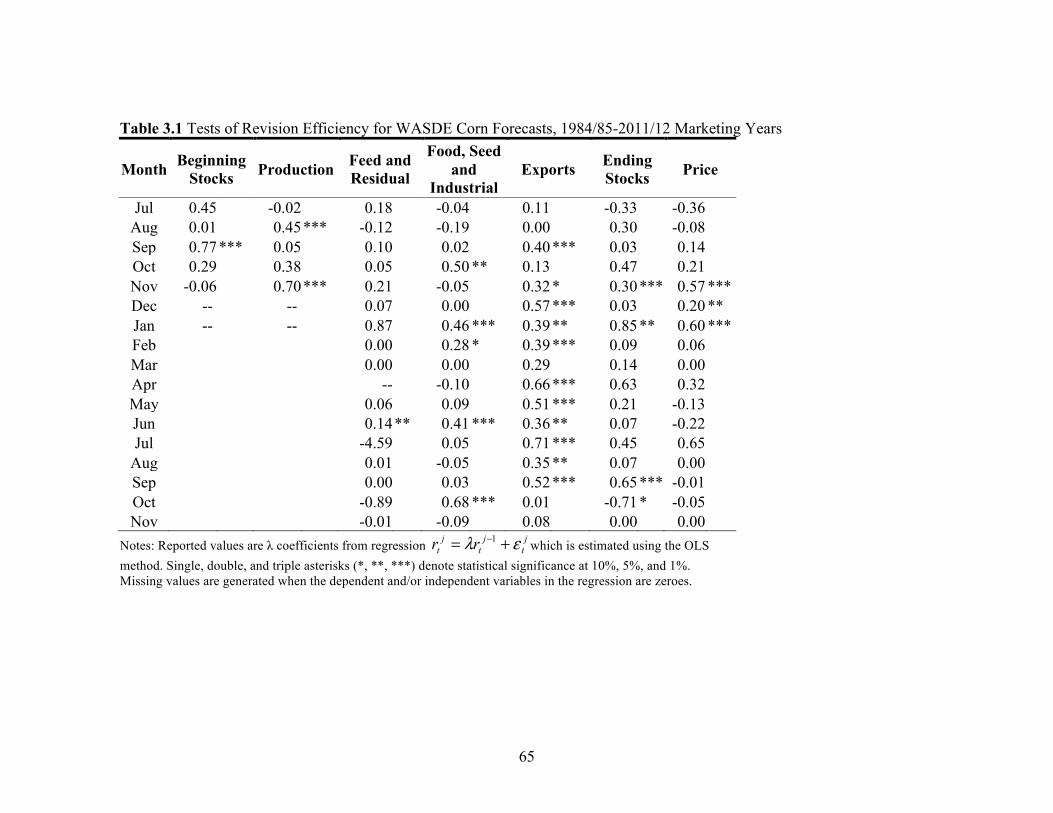
65
Table 3.1 Tests of Revision Efficiency for WASDE Corn Forecasts, 1984/85-2011/12 Marketing Years
Month Beginning Stocks Production Feed and
Residual
Food, Seed and
Industrial Exports Ending
Stocks Price
Jul 0.45 -0.02 0.18 -0.04 0.11 -0.33 -0.36 Aug 0.01 0.45 *** -0.12 -0.19 0.00 0.30 -0.08 Sep 0.77 *** 0.05 0.10 0.02 0.40 *** 0.03 0.14 Oct 0.29 0.38 0.05 0.50 ** 0.13 0.47 0.21 Nov -0.06 0.70 *** 0.21 -0.05 0.32 * 0.30 *** 0.57 *** Dec -- -- 0.07 0.00 0.57 *** 0.03 0.20 ** Jan -- -- 0.87 0.46 *** 0.39 ** 0.85 ** 0.60 *** Feb
0.00 0.28 * 0.39 *** 0.09 0.06
Mar 0.00 0.00 0.29 0.14 0.00 Apr -- -0.10 0.66 *** 0.63 0.32 May 0.06 0.09 0.51 *** 0.21 -0.13 Jun 0.14 ** 0.41 *** 0.36 ** 0.07 -0.22 Jul -4.59 0.05 0.71 *** 0.45 0.65
Aug 0.01 -0.05 0.35 ** 0.07 0.00 Sep 0.00 0.03 0.52 *** 0.65 *** -0.01 Oct -0.89 0.68 *** 0.01 -0.71 * -0.05 Nov -0.01 -0.09 0.08 0.00 0.00
Notes: Reported values are λ coefficients from regression which is estimated using the OLS method. Single, double, and triple asterisks (*, **, ***) denote statistical significance at 10%, 5%, and 1%. Missing values are generated when the dependent and/or independent variables in the regression are zeroes.
jt
jt
jt rr ελ += −1
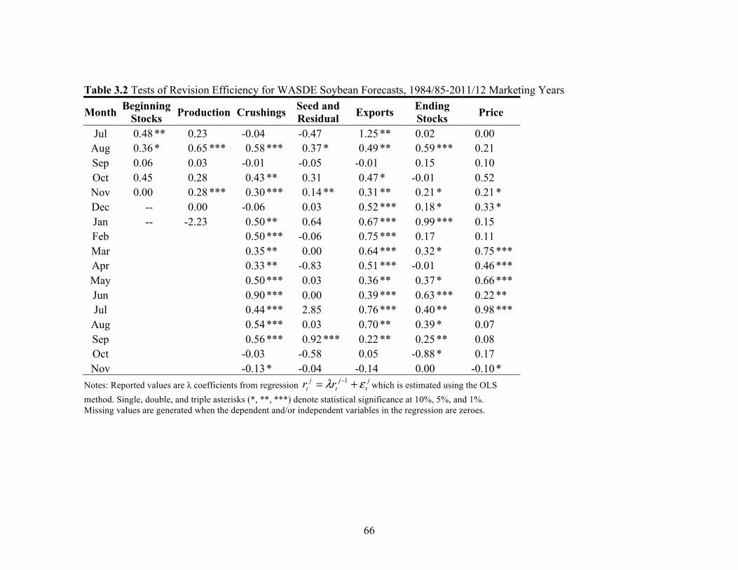
66
Table 3.2 Tests of Revision Efficiency for WASDE Soybean Forecasts, 1984/85-2011/12 Marketing Years
Month Beginning Stocks Production Crushings Seed and
Residual Exports Ending Stocks Price
Jul 0.48 ** 0.23 -0.04 -0.47 1.25 ** 0.02 0.00 Aug 0.36 * 0.65 *** 0.58 *** 0.37 * 0.49 ** 0.59 *** 0.21 Sep 0.06 0.03 -0.01 -0.05 -0.01 0.15 0.10 Oct 0.45 0.28 0.43 ** 0.31 0.47 * -0.01 0.52 Nov 0.00 0.28 *** 0.30 *** 0.14 ** 0.31 ** 0.21 * 0.21 * Dec -- 0.00 -0.06 0.03 0.52 *** 0.18 * 0.33 * Jan -- -2.23 0.50 ** 0.64 0.67 *** 0.99 *** 0.15 Feb 0.50 *** -0.06 0.75 *** 0.17 0.11 Mar 0.35 ** 0.00 0.64 *** 0.32 * 0.75 *** Apr 0.33 ** -0.83 0.51 *** -0.01 0.46 *** May 0.50 *** 0.03 0.36 ** 0.37 * 0.66 *** Jun 0.90 *** 0.00 0.39 *** 0.63 *** 0.22 ** Jul 0.44 *** 2.85 0.76 *** 0.40 ** 0.98 ***
Aug 0.54 *** 0.03 0.70 ** 0.39 * 0.07 Sep 0.56 *** 0.92 *** 0.22 ** 0.25 ** 0.08 Oct -0.03 -0.58 0.05 -0.88 * 0.17 Nov -0.13 * -0.04 -0.14 0.00 -0.10 *
Notes: Reported values are λ coefficients from regression which is estimated using the OLS method. Single, double, and triple asterisks (*, **, ***) denote statistical significance at 10%, 5%, and 1%. Missing values are generated when the dependent and/or independent variables in the regression are zeroes.
jt
jt
jt rr ελ += −1
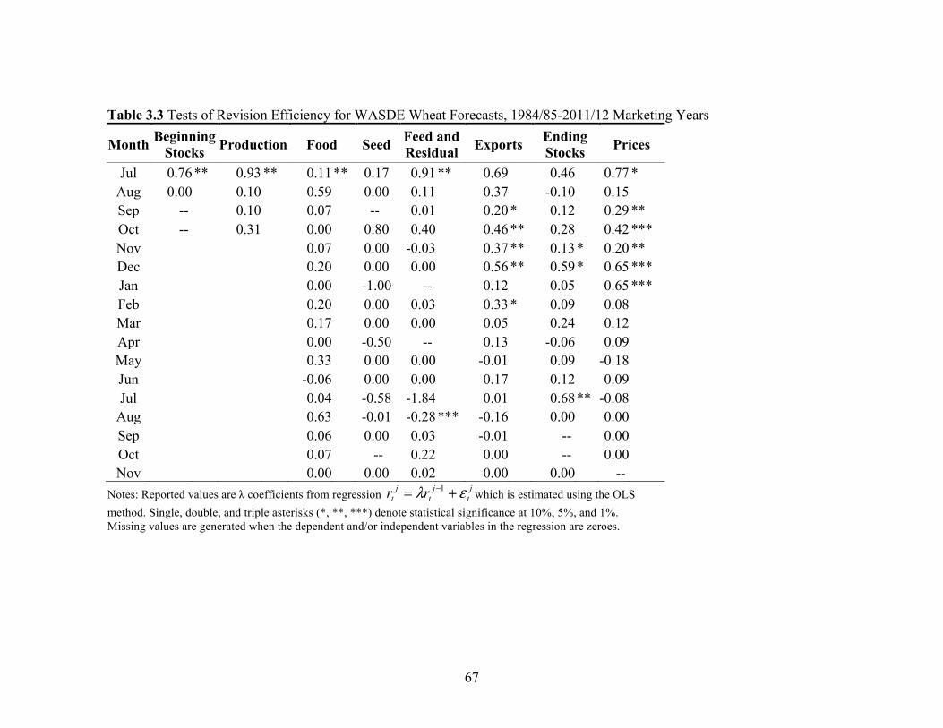
67
Table 3.3 Tests of Revision Efficiency for WASDE Wheat Forecasts, 1984/85-2011/12 Marketing Years
Month Beginning Stocks Production Food Seed Feed and
Residual Exports Ending Stocks Prices
Jul 0.76 ** 0.93 ** 0.11 ** 0.17 0.91 ** 0.69 0.46 0.77 * Aug 0.00 0.10 0.59 0.00 0.11 0.37 -0.10 0.15 Sep -- 0.10 0.07 -- 0.01 0.20 * 0.12 0.29 ** Oct -- 0.31 0.00 0.80 0.40 0.46 ** 0.28 0.42 *** Nov 0.07 0.00 -0.03 0.37 ** 0.13 * 0.20 ** Dec 0.20 0.00 0.00 0.56 ** 0.59 * 0.65 *** Jan 0.00 -1.00 -- 0.12 0.05 0.65 *** Feb 0.20 0.00 0.03 0.33 * 0.09 0.08 Mar 0.17 0.00 0.00 0.05 0.24 0.12 Apr 0.00 -0.50 -- 0.13 -0.06 0.09 May 0.33 0.00 0.00 -0.01 0.09 -0.18 Jun -0.06 0.00 0.00 0.17 0.12 0.09 Jul 0.04 -0.58 -1.84 0.01 0.68 ** -0.08
Aug 0.63 -0.01 -0.28 *** -0.16 0.00 0.00 Sep 0.06 0.00 0.03 -0.01 -- 0.00 Oct 0.07 -- 0.22 0.00 -- 0.00 Nov 0.00 0.00 0.02 0.00 0.00 --
Notes: Reported values are λ coefficients from regression which is estimated using the OLS method. Single, double, and triple asterisks (*, **, ***) denote statistical significance at 10%, 5%, and 1%. Missing values are generated when the dependent and/or independent variables in the regression are zeroes.
jt
jt
jt rr ελ += −1
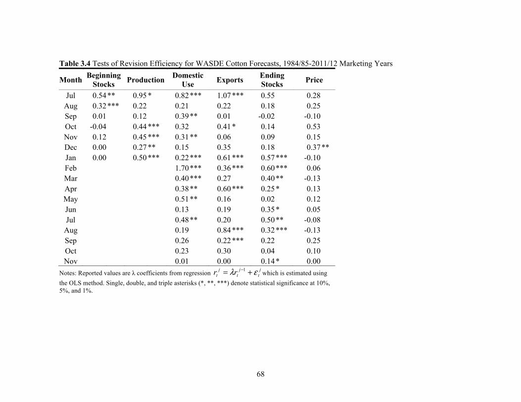
68
Table 3.4 Tests of Revision Efficiency for WASDE Cotton Forecasts, 1984/85-2011/12 Marketing Years
Month Beginning Stocks Production Domestic
Use Exports Ending Stocks Price
Jul 0.54 ** 0.95 * 0.82 *** 1.07 *** 0.55 0.28 Aug 0.32 *** 0.22 0.21 0.22 0.18 0.25 Sep 0.01 0.12 0.39 ** 0.01 -0.02 -0.10 Oct -0.04 0.44 *** 0.32 0.41 * 0.14 0.53 Nov 0.12 0.45 *** 0.31 ** 0.06 0.09 0.15 Dec 0.00 0.27 ** 0.15 0.35 0.18 0.37 ** Jan 0.00 0.50 *** 0.22 *** 0.61 *** 0.57 *** -0.10 Feb 1.70 *** 0.36 *** 0.60 *** 0.06 Mar 0.40 *** 0.27 0.40 ** -0.13 Apr 0.38 ** 0.60 *** 0.25 * 0.13 May 0.51 ** 0.16 0.02 0.12 Jun
0.13 0.19 0.35 * 0.05
Jul 0.48 ** 0.20 0.50 ** -0.08 Aug 0.19 0.84 *** 0.32 *** -0.13 Sep 0.26 0.22 *** 0.22 0.25 Oct 0.23 0.30 0.04 0.10 Nov 0.01 0.00 0.14 * 0.00
Notes: Reported values are λ coefficients from regression which is estimated using the OLS method. Single, double, and triple asterisks (*, **, ***) denote statistical significance at 10%, 5%, and 1%.
jt
jt
jt rr ελ += −1
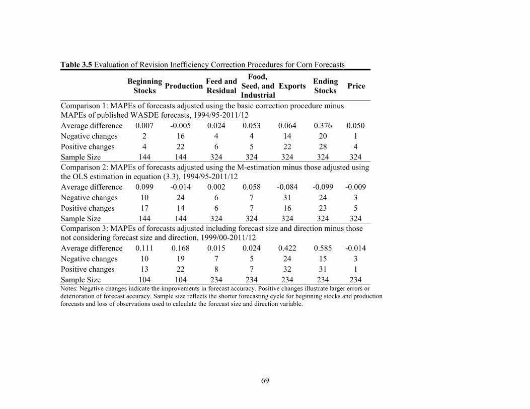
69
Table 3.5 Evaluation of Revision Inefficiency Correction Procedures for Corn Forecasts
Beginning
Stocks Production Feed and Residual
Food, Seed, and Industrial
Exports Ending Stocks Price
Comparison 1: MAPEs of forecasts adjusted using the basic correction procedure minus MAPEs of published WASDE forecasts, 1994/95-2011/12
Average difference 0.007 -0.005 0.024 0.053 0.064 0.376 0.050 Negative changes 2 16 4 4 14 20 1 Positive changes 4 22 6 5 22 28 4 Sample Size 144 144 324 324 324 324 324 Comparison 2: MAPEs of forecasts adjusted using the M-estimation minus those adjusted using the OLS estimation in equation (3.3), 1994/95-2011/12 Average difference 0.099 -0.014 0.002 0.058 -0.084 -0.099 -0.009 Negative changes 10 24 6 7 31 24 3 Positive changes 17 14 6 7 16 23 5 Sample Size 144 144 324 324 324 324 324 Comparison 3: MAPEs of forecasts adjusted including forecast size and direction minus those not considering forecast size and direction, 1999/00-2011/12
Average difference 0.111 0.168 0.015 0.024 0.422 0.585 -0.014 Negative changes 10 19 7 5 24 15 3 Positive changes 13 22 8 7 32 31 1 Sample Size 104 104 234 234 234 234 234 Notes: Negative changes indicate the improvements in forecast accuracy. Positive changes illustrate larger errors or deterioration of forecast accuracy. Sample size reflects the shorter forecasting cycle for beginning stocks and production forecasts and loss of observations used to calculate the forecast size and direction variable.
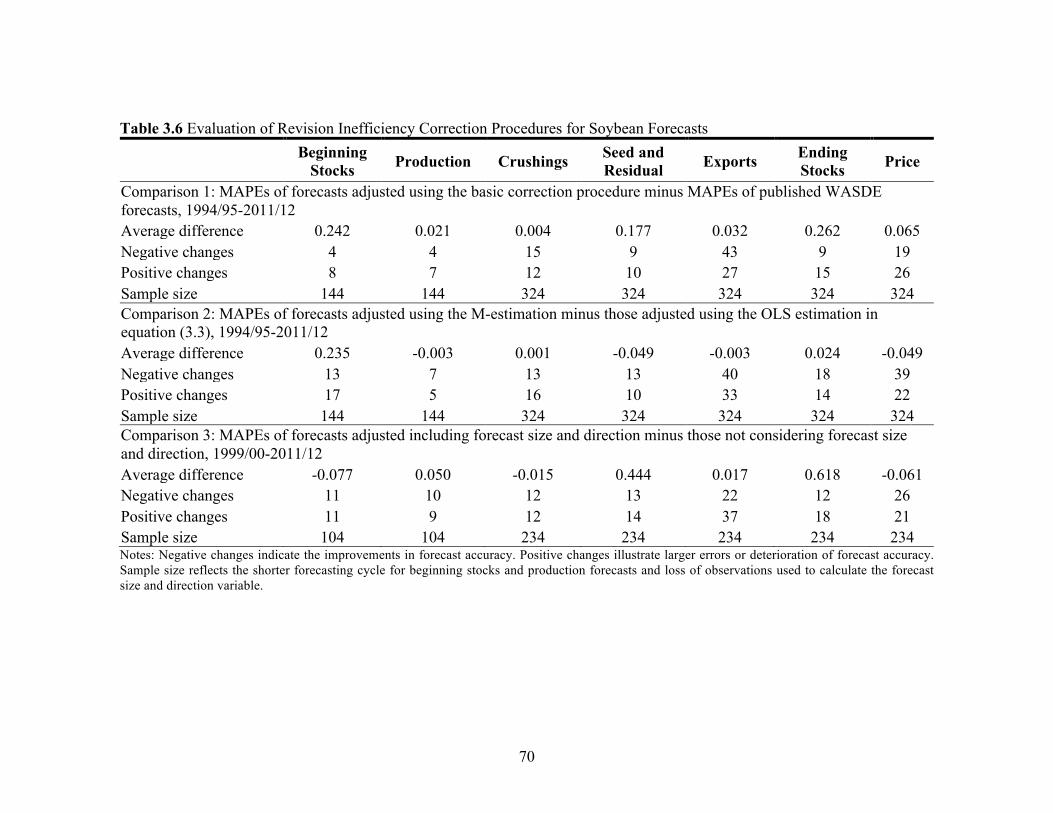
70
Table 3.6 Evaluation of Revision Inefficiency Correction Procedures for Soybean Forecasts
Beginning
Stocks Production Crushings Seed and Residual Exports Ending
Stocks Price
Comparison 1: MAPEs of forecasts adjusted using the basic correction procedure minus MAPEs of published WASDE forecasts, 1994/95-2011/12 Average difference 0.242 0.021 0.004 0.177 0.032 0.262 0.065 Negative changes 4 4 15 9 43 9 19 Positive changes 8 7 12 10 27 15 26 Sample size 144 144 324 324 324 324 324 Comparison 2: MAPEs of forecasts adjusted using the M-estimation minus those adjusted using the OLS estimation in equation (3.3), 1994/95-2011/12
Average difference 0.235 -0.003 0.001 -0.049 -0.003 0.024 -0.049 Negative changes 13 7 13 13 40 18 39 Positive changes 17 5 16 10 33 14 22 Sample size 144 144 324 324 324 324 324 Comparison 3: MAPEs of forecasts adjusted including forecast size and direction minus those not considering forecast size and direction, 1999/00-2011/12
Average difference -0.077 0.050 -0.015 0.444 0.017 0.618 -0.061 Negative changes 11 10 12 13 22 12 26 Positive changes 11 9 12 14 37 18 21 Sample size 104 104 234 234 234 234 234 Notes: Negative changes indicate the improvements in forecast accuracy. Positive changes illustrate larger errors or deterioration of forecast accuracy. Sample size reflects the shorter forecasting cycle for beginning stocks and production forecasts and loss of observations used to calculate the forecast size and direction variable.
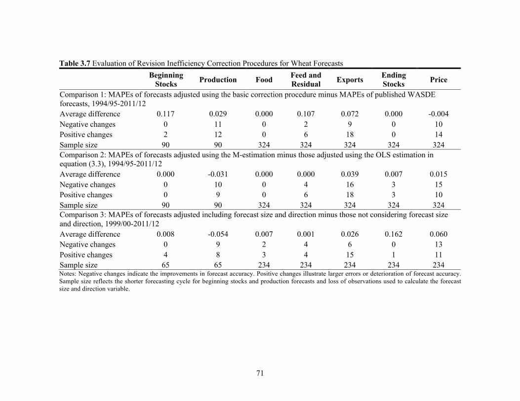
71
Table 3.7 Evaluation of Revision Inefficiency Correction Procedures for Wheat Forecasts
Beginning
Stocks Production Food Feed and Residual Exports Ending
Stocks Price
Comparison 1: MAPEs of forecasts adjusted using the basic correction procedure minus MAPEs of published WASDE forecasts, 1994/95-2011/12 Average difference 0.117 0.029 0.000 0.107 0.072 0.000 -0.004 Negative changes 0 11 0 2 9 0 10 Positive changes 2 12 0 6 18 0 14 Sample size 90 90 324 324 324 324 324 Comparison 2: MAPEs of forecasts adjusted using the M-estimation minus those adjusted using the OLS estimation in equation (3.3), 1994/95-2011/12 Average difference 0.000 -0.031 0.000 0.000 0.039 0.007 0.015 Negative changes 0 10 0 4 16 3 15 Positive changes 0 9 0 6 18 3 10 Sample size 90 90 324 324 324 324 324 Comparison 3: MAPEs of forecasts adjusted including forecast size and direction minus those not considering forecast size and direction, 1999/00-2011/12 Average difference 0.008 -0.054 0.007 0.001 0.026 0.162 0.060 Negative changes 0 9 2 4 6 0 13 Positive changes 4 8 3 4 15 1 11 Sample size 65 65 234 234 234 234 234 Notes: Negative changes indicate the improvements in forecast accuracy. Positive changes illustrate larger errors or deterioration of forecast accuracy. Sample size reflects the shorter forecasting cycle for beginning stocks and production forecasts and loss of observations used to calculate the forecast size and direction variable.
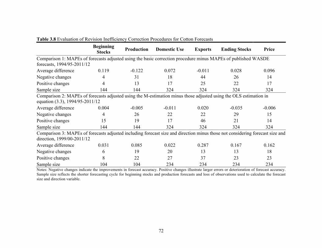
72
Table 3.8 Evaluation of Revision Inefficiency Correction Procedures for Cotton Forecasts
Beginning
Stocks Production Domestic Use Exports Ending Stocks Price
Comparison 1: MAPEs of forecasts adjusted using the basic correction procedure minus MAPEs of published WASDE forecasts, 1994/95-2011/12 Average difference 0.119 -0.122 0.072 -0.011 0.028 0.096 Negative changes 4 31 18 44 26 14 Positive changes 4 13 17 25 22 17 Sample size 144 144 324 324 324 324 Comparison 2: MAPEs of forecasts adjusted using the M-estimation minus those adjusted using the OLS estimation in equation (3.3), 1994/95-2011/12 Average difference 0.004 -0.005 -0.011 0.020 -0.035 -0.006 Negative changes 4 26 22 22 29 15 Positive changes 15 19 17 46 21 14 Sample size 144 144 324 324 324 324 Comparison 3: MAPEs of forecasts adjusted including forecast size and direction minus those not considering forecast size and direction, 1999/00-2011/12 Average difference 0.031 0.085 0.022 0.287 0.167 0.162 Negative changes 6 19 20 13 13 18 Positive changes 8 22 27 37 23 23 Sample size 104 104 234 234 234 234 Notes: Negative changes indicate the improvements in forecast accuracy. Positive changes illustrate larger errors or deterioration of forecast accuracy. Sample size reflects the shorter forecasting cycle for beginning stocks and production forecasts and loss of observations used to calculate the forecast size and direction variable.
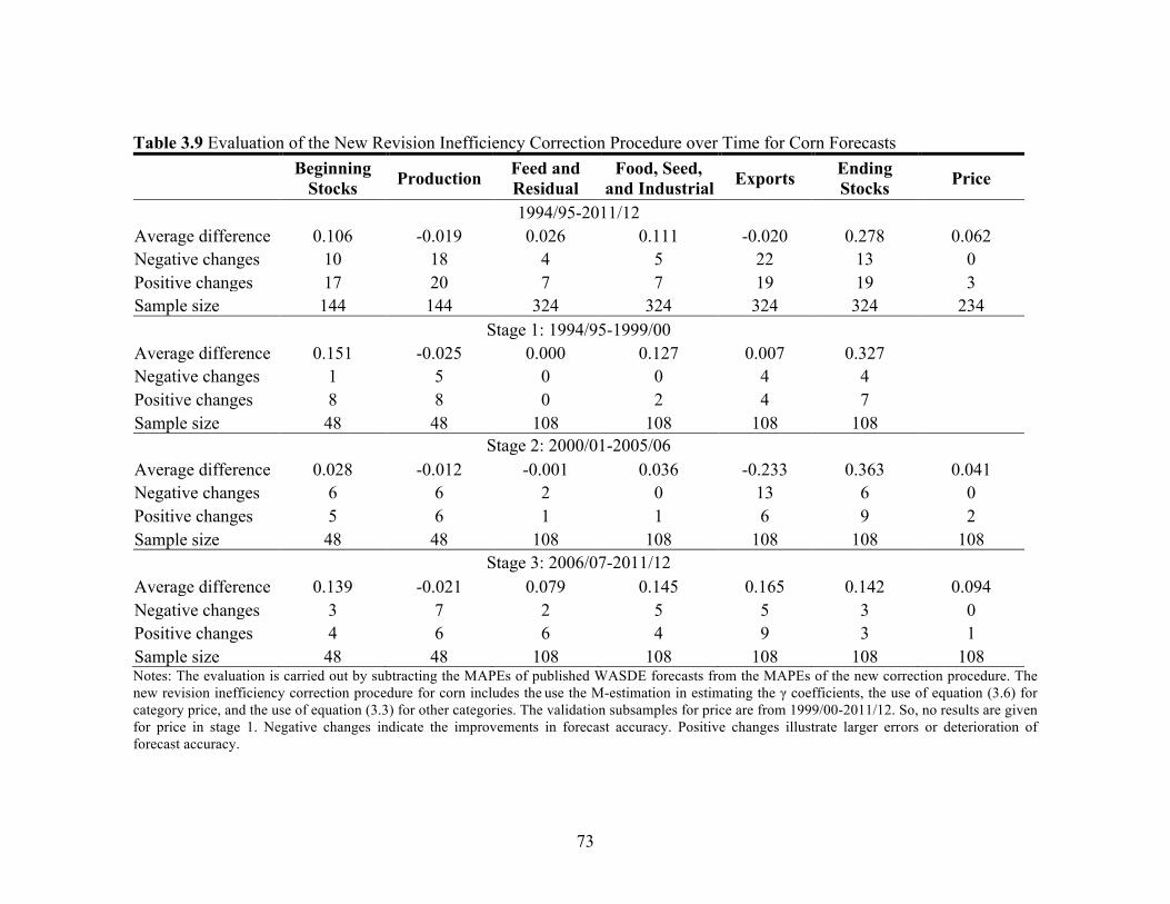
73
Table 3.9 Evaluation of the New Revision Inefficiency Correction Procedure over Time for Corn Forecasts
Beginning
Stocks Production Feed and Residual
Food, Seed, and Industrial Exports Ending
Stocks Price
1994/95-2011/12 Average difference 0.106 -0.019 0.026 0.111 -0.020 0.278 0.062 Negative changes 10 18 4 5 22 13 0 Positive changes 17 20 7 7 19 19 3 Sample size 144 144 324 324 324 324 234
Stage 1: 1994/95-1999/00 Average difference 0.151 -0.025 0.000 0.127 0.007 0.327 Negative changes 1 5 0 0 4 4 Positive changes 8 8 0 2 4 7 Sample size 48 48 108 108 108 108
Stage 2: 2000/01-2005/06
Average difference 0.028 -0.012 -0.001 0.036 -0.233 0.363 0.041 Negative changes 6 6 2 0 13 6 0 Positive changes 5 6 1 1 6 9 2 Sample size 48 48 108 108 108 108 108
Stage 3: 2006/07-2011/12
Average difference 0.139 -0.021 0.079 0.145 0.165 0.142 0.094 Negative changes 3 7 2 5 5 3 0 Positive changes 4 6 6 4 9 3 1 Sample size 48 48 108 108 108 108 108 Notes: The evaluation is carried out by subtracting the MAPEs of published WASDE forecasts from the MAPEs of the new correction procedure. The new revision inefficiency correction procedure for corn includes the use the M-estimation in estimating the γ coefficients, the use of equation (3.6) for category price, and the use of equation (3.3) for other categories. The validation subsamples for price are from 1999/00-2011/12. So, no results are given for price in stage 1. Negative changes indicate the improvements in forecast accuracy. Positive changes illustrate larger errors or deterioration of forecast accuracy.
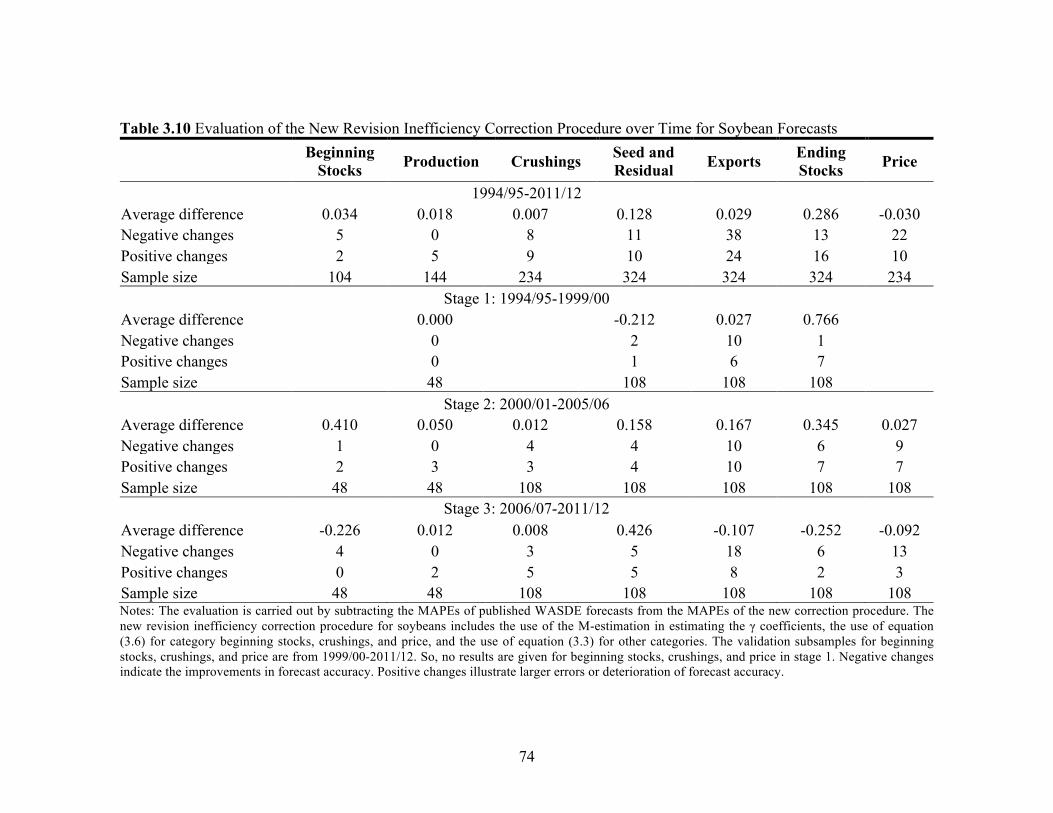
74
Table 3.10 Evaluation of the New Revision Inefficiency Correction Procedure over Time for Soybean Forecasts
Beginning
Stocks Production Crushings Seed and Residual Exports Ending
Stocks Price
1994/95-2011/12 Average difference 0.034 0.018 0.007 0.128 0.029 0.286 -0.030 Negative changes 5 0 8 11 38 13 22 Positive changes 2 5 9 10 24 16 10 Sample size 104 144 234 324 324 324 234
Stage 1: 1994/95-1999/00 Average difference 0.000 -0.212 0.027 0.766 Negative changes 0 2 10 1 Positive changes 0 1 6 7 Sample size 48 108 108 108
Stage 2: 2000/01-2005/06
Average difference 0.410 0.050 0.012 0.158 0.167 0.345 0.027 Negative changes 1 0 4 4 10 6 9 Positive changes 2 3 3 4 10 7 7 Sample size 48 48 108 108 108 108 108
Stage 3: 2006/07-2011/12
Average difference -0.226 0.012 0.008 0.426 -0.107 -0.252 -0.092 Negative changes 4 0 3 5 18 6 13 Positive changes 0 2 5 5 8 2 3 Sample size 48 48 108 108 108 108 108 Notes: The evaluation is carried out by subtracting the MAPEs of published WASDE forecasts from the MAPEs of the new correction procedure. The new revision inefficiency correction procedure for soybeans includes the use of the M-estimation in estimating the γ coefficients, the use of equation (3.6) for category beginning stocks, crushings, and price, and the use of equation (3.3) for other categories. The validation subsamples for beginning stocks, crushings, and price are from 1999/00-2011/12. So, no results are given for beginning stocks, crushings, and price in stage 1. Negative changes indicate the improvements in forecast accuracy. Positive changes illustrate larger errors or deterioration of forecast accuracy.
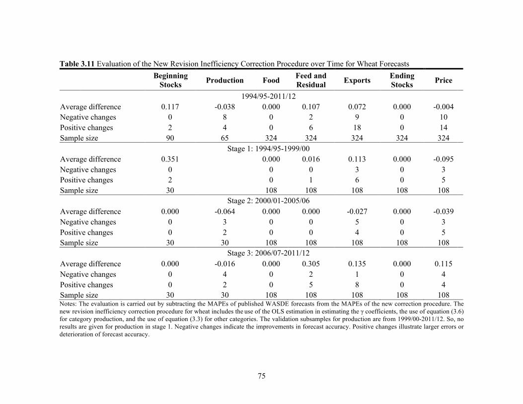
75
Table 3.11 Evaluation of the New Revision Inefficiency Correction Procedure over Time for Wheat Forecasts
Beginning
Stocks Production Food Feed and Residual Exports Ending
Stocks Price
1994/95-2011/12 Average difference 0.117 -0.038 0.000 0.107 0.072 0.000 -0.004 Negative changes 0 8 0 2 9 0 10 Positive changes 2 4 0 6 18 0 14 Sample size 90 65 324 324 324 324 324
Stage 1: 1994/95-1999/00 Average difference 0.351 0.000 0.016 0.113 0.000 -0.095 Negative changes 0 0 0 3 0 3 Positive changes 2 0 1 6 0 5 Sample size 30 108 108 108 108 108
Stage 2: 2000/01-2005/06 Average difference 0.000 -0.064 0.000 0.000 -0.027 0.000 -0.039 Negative changes 0 3 0 0 5 0 3 Positive changes 0 2 0 0 4 0 5 Sample size 30 30 108 108 108 108 108
Stage 3: 2006/07-2011/12 Average difference 0.000 -0.016 0.000 0.305 0.135 0.000 0.115 Negative changes 0 4 0 2 1 0 4 Positive changes 0 2 0 5 8 0 4 Sample size 30 30 108 108 108 108 108 Notes: The evaluation is carried out by subtracting the MAPEs of published WASDE forecasts from the MAPEs of the new correction procedure. The new revision inefficiency correction procedure for wheat includes the use of the OLS estimation in estimating the γ coefficients, the use of equation (3.6) for category production, and the use of equation (3.3) for other categories. The validation subsamples for production are from 1999/00-2011/12. So, no results are given for production in stage 1. Negative changes indicate the improvements in forecast accuracy. Positive changes illustrate larger errors or deterioration of forecast accuracy.
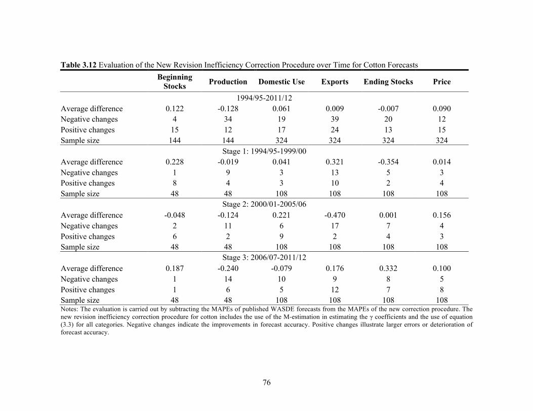
76
Table 3.12 Evaluation of the New Revision Inefficiency Correction Procedure over Time for Cotton Forecasts
Beginning
Stocks Production Domestic Use Exports Ending Stocks Price
1994/95-2011/12 Average difference 0.122 -0.128 0.061 0.009 -0.007 0.090 Negative changes 4 34 19 39 20 12 Positive changes 15 12 17 24 13 15 Sample size 144 144 324 324 324 324
Stage 1: 1994/95-1999/00 Average difference 0.228 -0.019 0.041 0.321 -0.354 0.014 Negative changes 1 9 3 13 5 3 Positive changes 8 4 3 10 2 4 Sample size 48 48 108 108 108 108
Stage 2: 2000/01-2005/06 Average difference -0.048 -0.124 0.221 -0.470 0.001 0.156 Negative changes 2 11 6 17 7 4 Positive changes 6 2 9 2 4 3 Sample size 48 48 108 108 108 108
Stage 3: 2006/07-2011/12 Average difference 0.187 -0.240 -0.079 0.176 0.332 0.100 Negative changes 1 14 10 9 8 5 Positive changes 1 6 5 12 7 8 Sample size 48 48 108 108 108 108 Notes: The evaluation is carried out by subtracting the MAPEs of published WASDE forecasts from the MAPEs of the new correction procedure. The new revision inefficiency correction procedure for cotton includes the use of the M-estimation in estimating the γ coefficients and the use of equation (3.3) for all categories. Negative changes indicate the improvements in forecast accuracy. Positive changes illustrate larger errors or deterioration of forecast accuracy.
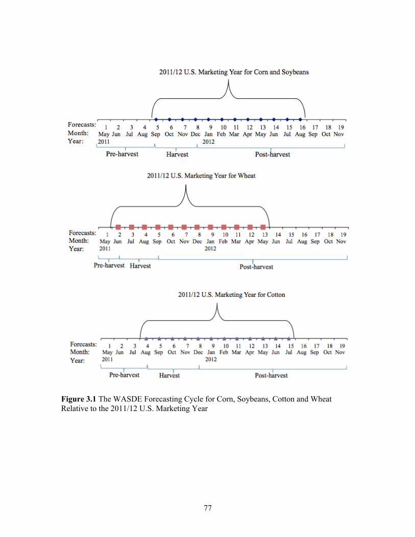
! 77
Figure 3.1 The WASDE Forecasting Cycle for Corn, Soybeans, Cotton and Wheat Relative to the 2011/12 U.S. Marketing Year
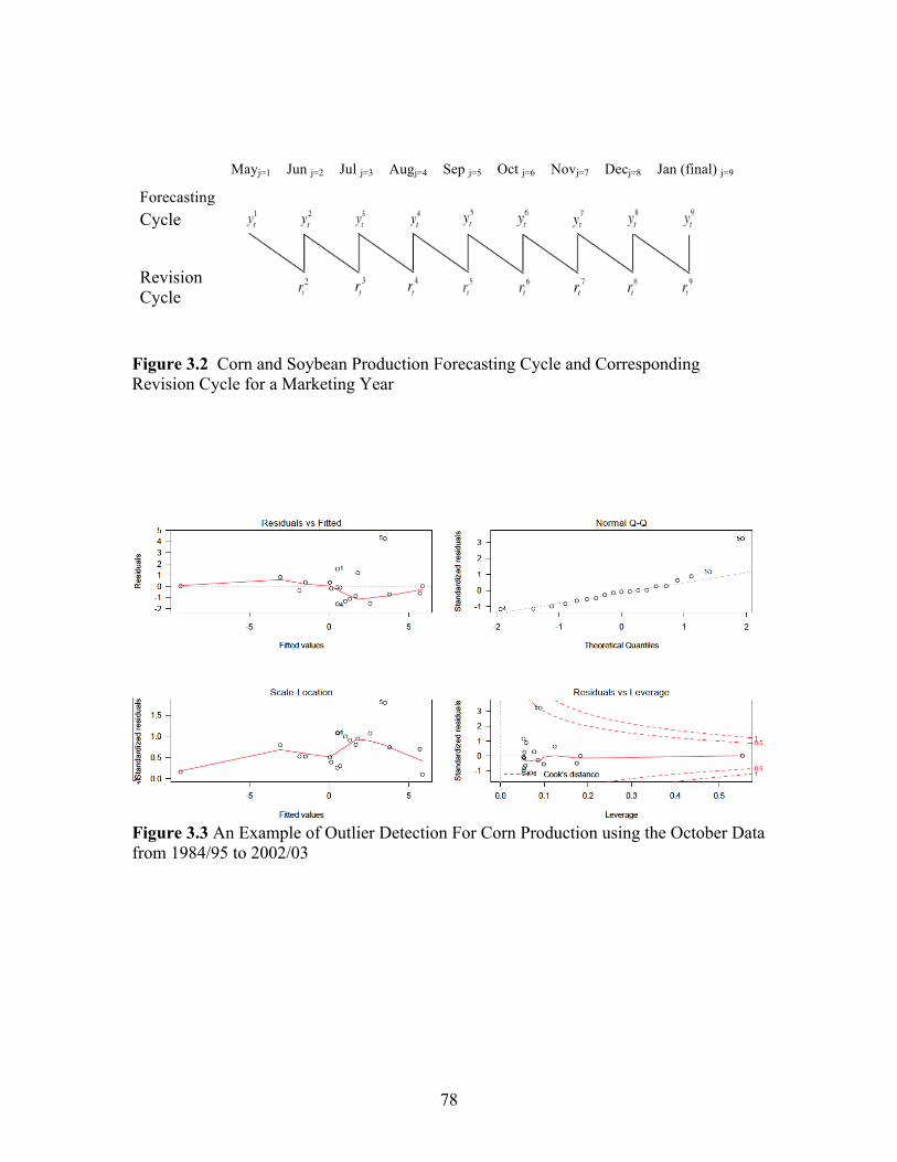
78
Forecasting
Mayj=1 Jun j=2 Jul j=3 Augj=4 Sep j=5 Oct j=6 Novj=7 Decj=8 Jan (final) j=9
Cycle
Revision Cycle
Figure 3.2 Corn and Soybean Production Forecasting Cycle and Corresponding Revision Cycle for a Marketing Year
Figure 3.3 An Example of Outlier Detection For Corn Production using the October Data from 1984/95 to 2002/03
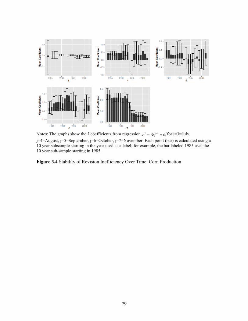
79
Notes: The graphs show the λ coefficients from regression for j=3=July, j=4=August, j=5=September, j=6=October, j=7=November. Each point (bar) is calculated using a 10 year subsample starting in the year used as a label; for example, the bar labeled 1985 uses the 10 year sub-sample starting in 1985. Figure 3.4 Stability of Revision Inefficiency Over Time: Corn Production
jt
jt
jt rr ελ += −1
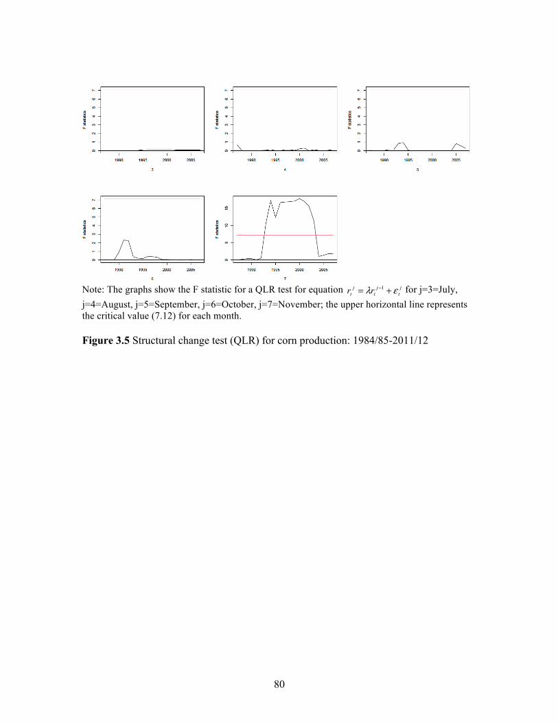
80
Note: The graphs show the F statistic for a QLR test for equation for j=3=July, j=4=August, j=5=September, j=6=October, j=7=November; the upper horizontal line represents the critical value (7.12) for each month. Figure 3.5 Structural change test (QLR) for corn production: 1984/85-2011/12
jt
jt
jt rr ελ += −1
81
CHAPTER FOUR
QUANTIFYING PUBLIC AND PRIVATE INFORMATION EFFECTS ON THE
COTTON MARKET
Introduction
In volatile agricultural markets, most public information is provided by the U.S.
Department of Agriculture (USDA), which historically devoted substantial resources to
their agricultural forecasting program (Offutt, 2002). Information in the USDA forecast
reports is widely used by farmers, agribusiness firms, other commercial decision makers,
speculators, as well as secondary information producers, such as universities, and
consulting and market advisory firms. Moreover, the importance of public information on
agricultural markets has been debated since the early 80s, given the emergence of private
agricultural analysis and the gradual reduction in governmental spending for statistical
reporting services. In comparison to public expenditure in 1980, 1983 federal budget
request for USDA was reduced by 20%. More recently, the USDA cut 12 statistical and
commodity reports in response to budgetary constraints in 2011 (NASS news, October
17, 2011), and in early 2013 USDA suspended a number of statistical surveys and reports
due to reduced funding (NASS news, March 12, 2013). Thus, the issue of the value of
public information sources has become particularly urgent.
Most previous studies evaluating public information effects focused on a single
report and provided mixed evidence. Sumner and Mueller (1989) found significant
announcement effect on corn and soybean market price movements using USDA harvest
forecast reports. McNew and Espinosa (1994) and Fortenbery and Sumner (1993) used
82
USDA Crop Production Report and reached a consistent conclusion that there is no
strong evidence indicating a significant influence USDA corn and soybean production
forecasts on the level of futures prices after 1985. In contrast, Garcia et al. (1997) and
Mckenzie (2008) analyzed the same USDA reports and suggested that corn and soybean
forecasts still provide valuable information on commodity futures markets, even though
there has been a reduction in the information effects after the mid-1980s. Colling and
Irwin (1990) and Mann and Dowen (1997) examined the effect of USDA Hogs and Pigs
Report and they found the ability of the futures market of hogs to incorporate
unanticipated information. Grunewald, McNulty, and Biere (1993) and Schaefer, Myers,
and Koontz (2004) discovered that live cattle futures prices respond to information
contained in Cattle on Feed Report.
The information effect of World Agricultural Supply and Demand
Estimates (WASDE), one of the most influential public sources of commodity forecasts,
has also been analyzed by several previous studies. Isengildina-Massa, Irwin, and Good
(2008a, 2008b) respectively investigated the impact of WASDE on the options and
futures price for corn and soybean. Both studies confirmed a significant price reaction to
the WASDE reports. More recently, Adjemian (2012) conducted a comprehensive study
by quantifing the WASDE information effect for multiple crop markets, and he found
significant impact. Although Dorfman and Karali (2013) analyzed multiple USDA
reports (Acreage & Prospective Plantings; Cattle; Cattle on Feed; Crop Progress; Feed
Outlook; Grain Stocks; Hogs and Pigs; Livestock, Dairy, and Poultry Outlook; Oil Crops
Outlook; and WASDE) within one study, they examined these reports separately using
83
parametric and nonparametric approaches. Report-by-report analysis does not allow the
measurement of the overall impact of a group of similar reports. More importantly,
evaluating a single report is likely to overestimate its effect since several public reports
could be simultaneously published within the same reaction window.
Isengildina, Irwin, and Good (2006) first studied to address the “clustering reports
problem” by simultaneously analyzing six USDA reports using a GARCH-type model.
They focused on the most influential reports in live hog and cattle returns. Later, Karali
(2012) evaluated the impact of multiple USDA reports on the conditional variances and
covariances of returns on 5 related futures contract.
Based on the above literature, we found most research has focused on the corn,
soybean, cattle, and hog markets, leaving the effect of public information on other
commodity market unclear. The objective of this study is to estimate the impact of all
major public reports and one private report on the cotton market from 1995 through 2012.
The cotton market was chosen because (a) the cotton industry has undergone substantial
changes over the last fifteen years (Isengildina and MacDonald, 2013); (b) cotton prices
have become particularly volatile in recent years (Robinson, 2009); (c) forecasts of cotton
prices were prohibited from 1929 to 2008; and (d) little is known about the impact of
information on cotton markets relative to other commodities.
Cotton daily futures returns of nearby futures contracts from January 1995
through January 2012 are used in the analysis. Reports identified as main sources of
public information for the cotton market include Crop Progress, Export Sales,
Perspective Plantings, and WASDE reports released by the USDA. This study also
84
includes the most commonly used private report: the Cotton This Month report from the
International Cotton Advisory Committee.24 Having both public and private reports
allows us to compare the impact of public and private information on the cotton market.
This study uses the standard event study approach, which has been widely used in
analyzing public information effect (e.g. Dorfman and Karali, 2013; Isengildina-Massa,
Irwin, and Good, 2006). Within this framework, information is considered valuable to
market participants if prices respond to the information release (the event). Evaluation of
the effect of multiple reports is then be conducted using the GARCH-type model similar
to the one outlined in Isengildina-Massa, Irwin, and Good (2006). The model controls for
other potential determinants of abnormal price movements, such as stock levels, day of
the week, seasonality, and weekend-holiday effects. This approach allows for valuation
of relative importance of five main reports in cotton futures market. Furthermore, the
methods reveal the report announcement effect on both the mean and the variance of
returns.
Data
Public and Private Reports
USDA, as the main public information provider, releases over 20 different reports
related to cotton industry each year. Moreover, other government-funded organizations,
such as International Cotton Advisory Committee (ICAC), National Cotton Council
24 The selection of main public reports on cotton has been discussed with Steven MacDonald, a senior economist in USDA, and John R. C. Robinson, professor and extension economist in Texas A&M University. !
85
(NCC), World Bank, and International Monetary Fund (IMF) publish various cotton
reports. Several reports identified in this study as main information sources for the cotton
market include Export Sales, Crop Progress, WASDE, and Perspective Plantings from
USDA and Cotton This Month from ICAC. Other reports, such as Cotton and Wool
Outlook and Weekly Cotton Market Review, contain mostly secondary information and
analysis and are not expected to move the markets.
Export Sales is published by the USDA through its export sales reporting system.
The reports are part of the USDA’s Export Sales Reporting Program, which monitors
U.S. agricultural exports on a daily and weekly basis. Only the weekly Export Sales
reports are included in this study; these reports are published every Thursday at 8:30 am
ET and contain the weekly summary of export activity for all major commodities. The
historical reports are available since November 1, 1990. Crop Progress reports list
planting, fruiting, and harvesting progress and overall condition of crops in major
producing states. The National Agricultural Statistics Service (NASS) issues weekly
Crop Progress reports during the growing season (early April through the end of
November or the beginning of December) of selected crops, including cotton, after 4:00
pm ET on the first business day of the week. The WASDE reports are released monthly
by the World Agricultural Outlook Board; they provide USDA's comprehensive
estimates and forecasts of supply and demand for major U.S. and global crops and U.S.
livestock to advise market participants about the current and expected market conditions.
Historically WASDE were published about one hour after the close of trading of cotton
futures. Starting in May 1994, the USDA changed the releasing time to 8:30 am ET.

86
Prospective Plantings reports are published at the end of March by the NASS every year
and concentrate on the expected plantings as of March 1st for various crops. Similar to
WASDE, Prospective Planting were scheduled to be released after market close before
1996 and the publishing time was switched to before market opening since 1996. ICAC
issues Cotton This Month reports at 3:00 pm ET of the first working day of each month in
five languages. These reports present estimates and projections of world supply and
demand and assessments of supply and demand by country. In contrast to other reports
included in this study, Cotton this Month is released to subscribers only.
The release of these five major reports in the cotton market represents “events” in
this study and is used to capture the impact of public reports on cotton futures prices. The
trading days immediately following reports release are considered event days. Thus, for
reports that are released after cotton futures market close, the event day is the day
following the release. On the other hand, the event day is equivalent to the release date if
a report is issued before trading hours. The event days for Cotton This Month, the only
private report included in this study, are the second day after the release of each month’s
report. The reason for using the second day25 instead of the first day is that the private
report releases to subscriber first and the new information takes longer to reach the
market.
Because the Crop Process reports can be only traced back to 1995, the sample
period for this study is chosen from January 1995 through January 2012. During the
sample period, weekly Export Sales and Crop Progress were published 893 and 598
25 This study also used the third days, forth days, and fifth days after the reports release as event days and the results are available upon requests.
87
times, respectively. Monthly WASDE reports were published 205 times and yearly
Prospective Plantings reports were published 17 times. ICAC released its first Cotton
This Month on November 1, 1995 and has published 194 reports since then. In total, 1907
public reports were included in this study. None of the five reports were intended to be
released on the same day, however, out of 1759 event days, 146 days and 1 day captures
the impact of two and three reports, respectively. This indicates the need to consider the
effect of “report clustering”.
Cotton Futures Returns
During the period of study, Cotton No. 2 futures contracts were traded on the New
York Board of Trade (NYBOT) and were operated under the CME Group. Cotton No. 2
has contract months of March, May, July, October, and December and the contract size is
50,000 pounds. To obtain a spliced, continuous price series for cotton, the closest to
delivery contract is used until the third Tuesday of the month prior to delivery, after
which the series switch to the next nearby contract. In this way, the expiration effects on
prices and on the level of trading activity are avoided. Table 4.1 presents the matching
futures contracts with each report release month.
The information effect in cotton futures market is measured in terms of returns.
Following previous studies by Yang and Brorsen (1993) and Isengildina-Massa, Irwin,
and Good (2006) returns are calculated as log percentage changes in the nearby futures
contract prices for cotton from January 3, 1995 through January 31, 2012. Accordingly,
the equation we use to calculate returns is:
(4.1) Rt = 100* (lnPt – lnPt-1),
88
where lnPt is the natural logarithm of the settlement price of cotton’s futures contract on
day t (event day), while Pt-1 is the settlement price on the previous day. This calculation
is also called the Close-to-Close (CTC) approach as the settlement prices are used in two
consecutive days. Karali (2012) stated “the advantage of using the CTC approach, as it is
more conservative if the impact is disseminated into prices instantaneously in the
opening”. However, Isengildina-Massa, Irwin and Good (2006) argued that CTC
measurement may mask the markets’ reaction to USDA reports as other information
becomes available to the market during the event day. Based on the efficient market
theory, which suggests the impact of new information should be reflected instantaneously
in futures prices right after a trading session begins, Isengildina-Massa, Irwin and Good
(2006) suggested using Close-to-Open (CTO) returns, and they also mentioned it is
necessary to use all three measures of returns--CTC, CTO, and open-to-close (OTC)--to
completely understand the dynamics of market reaction to USDA reports when the
reaction speed is unknown. Therefore, this study also calculates the returns in two other
ways: a) CTO returns, when Pt is the open price on the event day and Pt-1 is the
settlement price on the previous day; b) OTC returns (daily returns), where Pt and Pt-1 are
the event day’s settlement and open price, respectively.
Cotton futures contract is subject to daily price limit, which restricts potential
large price movements. Following previous studies (Park, 2000; Isengildina-Massa, Irwin,
and Good, 2006; Karali, 2012), this research does not adjust returns data for price limit
moves. Thus, the estimates of announcement effects may be underestimated because of
89
the lack of ability to detect large market reactions to new information in days with price
limit moves.
Descriptive Analysis
CTC, CTO, and OTC returns of cotton futures are respectively plotted in Panel 1-
3 of figure 4.1. Spikes can be seen in all three plots and they are related to the arrival of
important new information. This study evaluates if the five reports (Exports Sales, Crop
Process, WASDE, Perspective Plantings, and Cotton This Month) can be used to explain
the volatility in returns. Volatility of cotton futures markets is plotted in figure 4.2 in
terms of squared returns (a common measure of volatility, which emphasizes the
deviations of returns). The plots in Panels A and C show that CTC and OTC
measurements share a similar volatility pattern, where the returns were volatile in the
year of 2001 and 2009. However, the plot for CTO measurement indicates that the returns
of cotton futures market were most volatile around year 2005.26 All three plots in figure
4.2 suggest heteroskedasticity in variance (the volatility of returns) over time and they
show evidence of volatility clustering, indicating that low volatility was normally
followed by low volatility and vice versa.
Descriptive statistics for cotton futures returns are presented in table 4.2. The
average magnitude of returns is -0.03, -0.06, and 0.03 percentage points for CTC, CTO,
and OTC respectively. The skewness for all three measurements are between -0.5 and
0.5, suggesting the distribution of returns is approximately symmetric. The assumption
for normality is rejected in all three cases based on the Jarque-Bera test, and the rejection
26 Panel A, B, C in figure 4.2 have different scales. The largest volatility in Panel A is two times larger than the largest one in Panel B.
90
is likely to be explained by the large value for kurtosis. Although the values of kurtosis
for CTC and OTC returns are about half of the size for CTO, the kurtosis value is bigger
than 3, indicating the distribution of returns has a fatter tail than a normal distribution.
Methods
Traditional Ordinary Least Squares (OLS) method is not suitable to analyze
cotton’s daily futures returns because the distribution of returns is non-normal with time-
varying volatility as disscussed in the previous section. The GARCH-type models have
been widely used in commodity futures studies and they have been shown to more
accurately model the distribution of daily futures returns (e.g. Yang and Brorsen, 1993;
Yang and Brorsen, 1994; etc.). Selection of an appropriate GARCH model has always
been a great challenge, and there is no single GARCH-type model claimed as the best fit
for various commodities. Yang and Brorsen (1993) applied the GARCH(1,1) to capture
the nonlinear dynamics of 15 commodities’ daily futures price. One year later, they
compared three different models and concluded the GARCH(1,1)-t fits their data the best.
Isengildina-Massa, Irwin, and Good (2006) used a TARCH-in-mean model to measure
live/lean hog and live cattle futures returns as they found evidence that the markets react
asymmetrically to “good” and “bad” news. Instead of directly selecting a GARCH-type
model from previous literature, this study strives to select a GARCH model that best fits
the characteristics of the cotton futures daily returns. We first present the steps for
choosing an optimal GARCH model that fits the returns without any external effects. The
external effects, including public reports, are then added to build the full model.
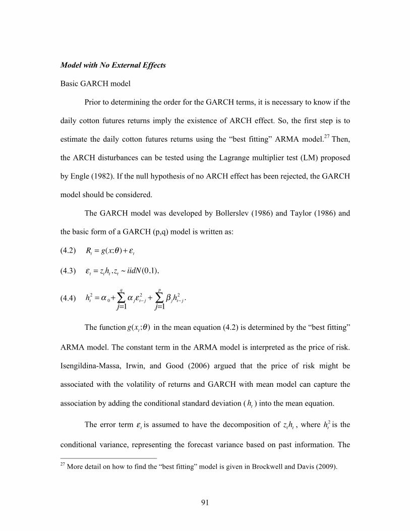
91
Model with No External Effects
Basic GARCH model
Prior to determining the order for the GARCH terms, it is necessary to know if the
daily cotton futures returns imply the existence of ARCH effect. So, the first step is to
estimate the daily cotton futures returns using the “best fitting” ARMA model.27 Then,
the ARCH disturbances can be tested using the Lagrange multiplier test (LM) proposed
by Engle (1982). If the null hypothesis of no ARCH effect has been rejected, the GARCH
model should be considered.
The GARCH model was developed by Bollerslev (1986) and Taylor (1986) and
the basic form of a GARCH (p,q) model is written as:
(4.2) Rt = g(x;θ )+ ε t
(4.3)
(4.4)
The function in the mean equation (4.2) is determined by the “best fitting”
ARMA model. The constant term in the ARMA model is interpreted as the price of risk.
Isengildina-Massa, Irwin, and Good (2006) argued that the price of risk might be
associated with the volatility of returns and GARCH with mean model can capture the
association by adding the conditional standard deviation ( ) into the mean equation.
The error term is assumed to have the decomposition of , where is the
conditional variance, representing the forecast variance based on past information. The 27 More detail on how to find the “best fitting” model is given in Brockwell and Davis (2009).
ε t = ztht , zt ~ iidN(0,1),
ht2 =α 0+ α j
j=1
q
∑ ε t− j2 + β j
j=1
p
∑ ht− j2 .
g(xt ;θ )
ht
ε t ztht ht2

92
conditional variance is presented as a function of a constant term ( ), the new
information measured as the sum of squared previous days’ returns ( ), and the
previous forecast variances ( ). Coefficients of GARCH model are normally
estimated by the maximum likelihood estimation (MLE) method using the algorithm
developed by Marquardt (1963).
As stated by Teräsvirta, Tjøstheim and Granger (2011), the overwhelmingly most
popular GARCH model in applications has been the GARCH(1,1) model, where p=q=1
in equation (4.4). In addition, Hansen and Lunde (2005) compared 330 different volatility
models using daily exchange rate data (DM/$) and IBM stock prices and they concluded
that the GARCH(1,1) was not significantly outperformed by any complicated GARCH
models. Therefore, GARCH(1,1) is a good starting point to fit the daily cotton futures
returns data. The LM test can be applied again for testing the existence of left over
ARCH effects and higher order GARCH model will be considered if the null hypothesis
is rejected.
Extensions of basic GARCH model have been developed to deal with “stylized
facts”, including asymmetric, non-gaussian error distribution, and long memory, in
financial and agricultural commodity time series data. Our approach to incorporating
these additional factors in the daily cotton futures returns is described in the following
sections.
α 0
α jj=1
q
∑ ε t− j2
β jj=1
p
∑ ht− j2

93
GARCH Model with Non-Gaussian Error Distribution
In the basic GARCH model, the error term follows a normal distribution (see
equation 4.3). Even though the distribution of financial and commodity returns have
fatter tail than a normal distribution, He and Teräsvirta (1999) argue that a GARCH
model with normal errors (GARCH-normal) can replicate some fat-tailed behavior.
However, due to the high kurtosis values (4.50, 10.03, and 5.24 for CTC, CTO and OTC
returns, respectively), it is important to consider distributions with fatter tails than the
normal distribution. Zivot (2009) notes that the commonly used fat-tailed distributions for
fitting GARCH models include the Student’s t distribution, the double exponential
distribution, and the generalized error distribution.
GARCH model with Student’s t distribution (GARCH-t) is considered in this
study. Bollerslev (1987) first developed the GARCH-t, and the GARCH-t process is
claimed to be useful in modeling leptokurtosis as it features both conditional
heteroskedasticity and conditional leptokurtosis (Yang and Brorsen, 1994). For a
GARCH-t model, the error term in the GARCH model follows a Student’s t
distribution with degrees of freedom (Bollerslev, 1987). After the GARCH-t model has
been fit to the data, the adequacy of assuming Student’s t distribution can be tested
graphically by plotting the quantile-quantile plot (QQ plot) with the standardized
residuals because the distribution of the standardized residuals should match the specified
error distribution used in the estimation (Zivot, 2009).
Asymmetric GARCH Model
In the basic GARCH model, the signs of the residuals ( ) have no impact on the
ε t
v
ε t

94
conditional variance ( ) because only the squared residuals are included in equation
(4.4). However, previous literature suggests that “bad” news (when previous returns are
negative) tends to have a larger effect on volatility than “good” news (when previous
returns are positive) (e.g. Engle, 2004; Isengildina-Massa, Irwin, and Good, 2006). In
other word, the reaction of volatility toward different types of news is asymmetric.
Therefore, it is necessary to examine if such asymmetric reactions exist in the cotton
daily futures returns.
Asymmetry can be tested by calculating the correlation between the squared
return and lagged return . Negative correlation suggests the existence of
asymmetry (Zivot, 2009). If asymmetry in the daily cotton futures returns has been
identified, an asymmetric volatility model such as EGARCH (Nelson, 1991), TGARCH
(Zakoian, 1994), and GJR-GARCH (Glosten, Jaggnnathan, and Runkle, 1993) may be
preferred to the basic GARCH model. Using TGARCH as an example, equation (4.4)
will be adjusted as:
(4.5)
where if or if . Therefore, for “bad” news, the total
effect of is given by , while for “good” news, the total effect of is
given solely by .
Long Memory GARCH Model
For many financial and agricultural commodity time series, the for the previous
ht2
Rt2 Rt−1
ht2 =α 0+ α j
j=1
q
∑ ε t− j2 + γ j It− j
j=1
q
∑ ε t− j2 + β j
j=1
p
∑ ht− j2 ,
It− j = 1 ε t− j2 < 0 It− j = 0 ε t− j ≥ 0
ε t− j2 (α j + γ j )ε t− j
2 ε t− j2
α jε t− j2
β1

95
period’s volatility in equation (4.4) is very close to 0.9 (e.g. Yang and Brorsen, 1994;
Hansen and Lunde 2001), indicating a large/small volatility is always followed by a
large/small volatility. This feature is identified as volatility persistence or volatility
clustering. The basic GARCH model captures this feature with an exponential decay in
the autocorrelation of conditional variance. However, it has been noticed that the squared
and absolute returns of financial assets have serial correlations that decays much slower
than an exponentially decay. To the best of our knowledge, previous studies in
agricultural commodity futures returns have not paid particular attention to this long
memory phenomenon.
In this study, plotting the autocorrelation function for the squared daily cotton
futures returns is used to check for the presence of the long memory behavior. If such
behavior exists, the Integrated GARCH (IGARCH) model will be applied to fit the
returns. IGARCH eliminates the intercept coefficient in equation (4.4) and restricts
the sum of all other and coefficients to be one (Engle and Bollerslev, 1986).28
Full Model with External Effects
Although the objective of this study is to identify the public information effect on
cotton futures market, it is necessary to account for other potential determinants of
market volatility while considering the impact of public reports. Well-documented
external factors include the day-of-the-week effects (e.g. Yang and Brorsen, 1994;
28 The IGARCH process is not weekly stationary as the unconditional variance does not exist. Nelson (1990) showed that the IGARCH(1,1) process is strongly stationary if
. Therefore, the parameters of the model can still be consistently estimated by MLE.
ht−12
α 0
α j β j
E ln(α1 + β1zt2 ) < 0
96
Isengildina-Massa, Irwin, and Good, 2006) and the seasonality in variance (e.g. Hennessy
and Wahl, 1996; Isengildina, Irwin, and Good, 2006). In addition, Williams and Wright
(1991) asserted a theoretical argument that market conditions affect the reaction of a
storable commodity’s price to announcements. And the “market conditions” had latter
been explained as commodity stock level or inventory conditions (Good and Irwin, 2006;
Colling, Irwin, and Zulauf, 1996; Adjemian, 2012).
The impact of external effects is commonly estimated by adding dummy variables
into the mean/or variance equations. In this study, the dummy variables for each day of
the week, including DT, Dw, DH and DF, with DM treated as the base category, are
included in both the mean equation (4.2) and the variance equation (4.4). Using DT as an
example, DT equals one if Tuesday and zero otherwise. Outlined in Isengildina-Massa,
Irwin, and Good (2006) and Karali (2012), seasonality is introduced into the variance
equation as 11 monthly dummy variables (DJAN for January, DFEB for February, DMAR for
March, DAPR for April, DMAY for May, DJUN for June, DJUL for July, DAUG for August,
DSEP for September, DOCT for October, DNOV for November) with DDEC for December as
the base categories. Monthly cotton stocks data (value of ending stocks, which is
recorded on the last day of the month) is drawn from the USDA Economic Research
Service’s Cotton and Wool Situation and Outlook Yearbook. The procedure to generate
the inventory level of each day is described in Adjemian (2012). He defined the stock
level on the report day of the first month (R) is SR and the stock on the report day of the
next month (N) is SN. Then the stock level for any day t between report days R and N is
calculated as:

97
(4.6)
The calculated daily stock levels can be then ordered by their magnitudes and the lowest
1/5th are recorded as low stock levels. The stock level effect is tested by adding a dummy
variable DLOW into the variance equation (4.4) directly. DLOW equals one if the daily stock
level is low and zero otherwise.
Following Isengildina-Massa, Irwin, and Good (2006) and Karali (2012), the
impact of public reports on cotton daily futures returns is measured only in the variance
equation. DES for Export Sales, DCP for Crop Progress, DWASDE for WASDE, DPP for
Perspective Plantings and DCTM for Cotton This Month reports are introduced as dummy
variables with the value of one on the event day and zero otherwise. We also include the
weekend-holiday effect, which we define as the impact of a public report release after the
futures market close on Friday or the day before a holiday. Since the futures market
closes during weekends and holidays, the markets have longer time to react to the new
information. We anticipate that the impact of public reports would be masked by this
weekend-holiday effect. Two dummies DHWCP and DHWCTM29
are generated and added
into the variance equation. These dummy variables equal one on the first day after the
weekends or holidays if the corresponding report releases after the futures market closes
on the previous Fridays or the day before holidays, and zero otherwise.
29 DHWES, DHWWASDE, and DHWPP are not included because the holiday-weekend effect does not apply to the Export Sales, WASDE, and Perspective Plantings reports.
St =SR if t=R
St−1 +SN − SR
N − R if R<t<N
.⎧
⎨⎪
⎩⎪
98
Results
Model Selection30
Although previous studies normally included ten lagged independent variables in
the mean equation (Yang and Brorsen, 1994; Isengildina-Massa, Irwin, and Good, 2006),
the “best fitting” ARMA model to estimate the daily cotton futures CTC returns was the
autoregressive process containing four lags, AR(4).31 Additionally, the null hypothesis of
no ARCH effect with lag of five32 was rejected at the significance level of 99%,
indicating the need for using a GARCH-type model.
The GARCH(1,1)-normal model was estimated first and the test statistics are
presented in the first column of table 4.3. No higher order of GARCH model was needed
as the LM test indicates there was no ARCH effect left after fitting the GARCH(1,1)-
normal. If the residuals are normally distributed, the standardized residuals in the QQ plot
should lie alongside a straight 45 degree line. However, the QQ plot in figure 4.3a of the
standardized residuals calculated based on the GARCH(1,1)-normal model indicates a
departure from normality as the points are off the straight line at both ends. This finding
implies the need for applying a distribution with fatter tails.
The GARCH(1,1)-t was then estimated and the test statistics can be found in the
second column of table 4.3. The LM test result was consistent with the one for
GARCH(1,1)-normal. The Akaike Information Criterion (AIC) and the Schwartz
Bayesian Criterion (SBC) for GARCH(1,1)-t were smaller than the ones for 30 Due to space limitation, the model selecting process is only explained in detail for the CTC returns. 31 Details on the selection of AR(4) is available upon request. 32 The null hypothesis of the Lagrange multiplier test with other lag values were also rejected.

99
GARCH(1,1)-normal, indicating that the GARCH(1,1)-t is preferred. In addition, the
standardized residuals computed after fitting the GARCH(1,1)-t that more closely
followed the straight line in the QQ plot in figure 4.3b suggesting that the GARCH(1,1)-t
was a better fit for cotton daily futures returns.
As described in the methodology section, asymmetry can be tested by examining
the correlation between the squared returns and lagged returns. The correlation between
these two variables was -0.02, which suggests no existence of asymmetry. Furthermore,
the insignificant asymmetric coefficient in equation (4.5) of the TGARCH-normal
model led to the same conclusion.
Figure 4.4 contains the autocorrelations (ACF) and partial autocorrelations
(PACF) plots of the squared CTC returns. Starting from lag one, the autocorrelations
decayed much slower than an exponentially decay expected for a GARCH model. In
addition, the sum of the GARCH coefficients and for GARCH(1,1)-t was very
close to one. Both findings indicated that the daily cotton futures returns have the long
memory behavior. Therefore, the IGARCH(1,1)-t was fitted next to capture the strong
persistence in the returns’ variance and the test statistics are reported in the third column
of table 4.3. Due to this change, that the intercept in the variance equation was eliminated
while the other GARCH coefficients were forced to add up to one. Although the log-
likelihood was reduced from -8063.34 (from GARCH(1,1)-t) to -8071.01, which implies
a log-likelihood ratio test statistic of 15.34 with two degree of freedom, Engle and
Bollerslev (1986) argued that this reduction is mainly due to the restriction of setting
intercept to be zero. The QQ plot for IGARCH(1,1)-t in Figure 4.3 demonstrate that
γ
α1 β1
100
IGARCH(1,1)-t is preferred to GARCH(1,1)-t as the standard residuals follows the
straight line in figure 4.3c closer than in 3b.
GARCH(1,1)-t with mean was also tested and the results are reported in the last
column of table 4.3. Neither the coefficient for nor the log-likelihood ratio statistic was
significant, indicating the conditional standard deviation should not be included in the
mean equation (4.2).
Based on the results in table 4.3, the best fitting model for daily cotton futures
CTC, CTO, OTC returns were AR(4)-IGARCH(1,1)-t, AR(4)-GARCH(1,1)-t with mean,
and AR(7)-IGARCH(1,1)-t, respectively.
Full Model for CTC Returns33
The first column in table 4.4 presents the results for CTC returns including all
external effects (the day-of-week effect both in the mean and variance equation, the
seasonality effect, reports effect, stock level effect, and weekend-holiday effect in the
variance equation). Autocorrelation was significant in the second and the forth lags.
Because the external effects were introduced through a series of dummy variables, the
estimates need to be interpreted relative to the base alternative of a no-report Monday in
December with a high stock level. Wednesday returns appeared to be 0.144 percentage
points higher than Monday returns and cotton futures were less volatile on Wednesdays
and Fridays. Seasonality can be found in May and September where cotton futures were
significantly more volatile in these two months than in December. The stock level effect
and weekend-holiday effect were both insignificant. The GARCH coefficients in the 33 Because of the space limitation, the impacts of external effects, especially the information effect, were explained focusing on the CTC returns.
ht
101
variance equation suggest that the conditional variance of cotton futures placed a weight
of about 95.3% on the prior day’s conditional variance estimate and a weight of 4.7% on
the previous day’s information about returns.
Impacts of Public and Private Reports
According to the results in the column 1 of table 4.4, the coefficients of the
dummy variables are positive for most reports except Crop Process. Positive signs
indicate USDA reports increase the conditional variance of returns on the event day, and
under market efficiency, provide new information to the market. Among the five reports,
WASDE and Perspective Planting reports had a significant impact on cotton futures CTC
returns. The release of WASDE and Perspective Planting report increased the conditional
variance by a factor of 0.5827 and 0.8468, respectively. The only private report included
in the study, Cotton This Month, did not significantly affect the cotton market.
Since return volatility in agricultural market was often perceived in terms of
standard deviation, Isengildina-Massa, Irwin and Good (2006) suggested interpreting the
impact of reports relative to the estimated average standard deviation of the daily futures
returns. Therefore, the coefficients in table 4.4 can be translated to changes in standard
deviation of the underlying futures returns using the comparative statistic equation:
(4.7) ,
where is the estimated coefficient for each report and the proxy of is the estimated
mean conditional variance from the IGARCH(1,1)-t model. According to the results in
table 4.5, the mean estimated conditional standard deviation was 1.75%. The coefficients
∂ht∂Di
= ∂ht∂ht
2 ×∂ht
2
∂Di
= 12ht
×δ i =δ i
2ht
δ i ht
102
in table 4.5 were drawn from the first column of table 4.4 and the partial derivative
can be interpreted as the increase in the conditional standard deviation of cotton
futures CTC returns associated with the release of a report, given all other external
factors constant. For example, the partial derivative for Perspective Planting is 0.248
(calculated by ), indicates that the conditional standard deviation of cotton
futures returns increased by 0.248 percentage points on average because of the release of
a Perspective Planting report. The proportion of the mean in table 4.5 represents the
increase in conditional standard deviation due to report release expressed as a proportion
of the mean conditional standard deviation. For example, the conditional standard
deviation of cotton futures returns was 14.6% (0.248/1.705) greater on the release days of
Perspective Planting reports. The release of WASDE also significantly increased the
mean conditional standard deviation by about 10%.
Following Adjemian (2012), the impact of information can be explained one step
further, in the context of a holder of cotton futures contract, measured against the size of
the maintenance margin. The maintenance margin is the minimum amount of collateral
that has to be posted in an account for a futures position to remain open. Currently,
IntercontinentalExchange requires $1,750 for a speculative or hedge trader and the size of
the cotton futures contract is 50,000 pounds. Results in table 4.6 illustrate the impact of
report release on market participants. At the mean settle price of $0.673 per pound during
our sample period, WASDE reports moved cotton prices by an average of $0.0012
(0.673*0.171) per pound. In terms of the futures contract, the WASDE shifted the value of
∂ht / ∂Di
0.86482 ×1.705
ht
103
each contract (up or down) by an average of $57.5 ($0.0012*50,000 pounds), which
represents a 3.29% ($57.5/$1,750) of collateral tied up in a position. On the other hand,
the release of Perspective Planting report resulted in a 4.77% change in the collateral.
Similar interpretation using the maximum settle price of cotton $2.14 per pound showed
that the release of WASDE and Perspective Planting reports could change the value of a
cotton futures contract by as much as $182.8 and $265.7—a 10.45% and 15.18% return
on collateral, respectively.
WASDE is considered one of the most valuable forecasting reports for agricultural
commodity and its value has been analyzed by multiple studies. It is useful to find out if
prices react differently to WASDE reports released at various times within a year.
Therefore, the interaction terms for Monthly effects with WASDE dummies were
included in the full model and the results are reported in the column 2 of table 4.4. The
monthly effects of WASDE reports are also plotted in figure 4.5. Based on the results, the
September WASDE report had the largest significant impact on price volatility as it
increased the conditional variance of the CTC returns by 1.74 percentage point
comparing with a non-WASDE event day in December, given other external factors
constant.
Column 3 of table 4.4 presents the results with only WASDE in the model. The
significant coefficient for the WASDE report was 0.6501, which was higher than the
coefficient in the column 1 of that table, proving that evaluating WASDE reports
separately overestimates their effects due to “clustering”. The extent of clustering in our
104
sample is 67 out of 205 WASDE event days, when one or two other reports were also
published.
Comparison of results for CTC, CTO, and OTC returns
While table 4.4 presents the results of the full model with all external effects (day-
of-week, seasonality, stock level, weekend-holiday, and reports effect) for CTC returns,
table 4.7 reports the model with selective external effects for CTC, CTO, and OTC
returns. The external factors were chosen if they improved the fit of the model
significantly using a series of log-likelihood ratio tests. Different “best fitting” models
were applied for various returns as described in a previous section. According to the
results, the day-of-week effect was included both in the mean and variance equations for
CTC and OTC returns, while it was only added in the variance equation for CTO returns.
The weekend-holiday effect for Crop Process report was included only in CTO and OTC
returns.
Impacts of Public and Private Reports
All CTC, CTO, and OTC returns were used in the study to demonstrate the
progression of market reaction to new information. Isengildina-Massa, Irwin, and Good
(2006) discussed the three different patterns of market reaction. First, under market
efficiency, futures price may reach a new equilibrium shortly after the release of new
information between trading sessions. In this case, CTO returns would reflect the full
impact of the new information while the OTC returns would reflect no impact and the
CTC returns would reflect the impact dampened by additional information arriving in the
market during the trading day. The second scenario is when the market is not efficient
105
and tends to over-react to new information, and the third scenario is when the market
reacts to new information but not instantaneously. If the market reaction follows the
second or third scenarios, the initial reaction (open price of the event day) should not be
used, and the CTC returns would reflect the true equilibrium.
The coefficient results in table 4.7 show that the WASDE effect was significant
using the CTO and CTC returns while the impact of Perspective Planting was significant
using the CTC and OTC returns. Interestingly, the impact of the only private report,
Cotton this Month, was also significant in the OTC returns.
Notice that the magnitudes of coefficients can be only compared within one type
of returns. The comparisons among different returns need to be conducted by using the
ratios of coefficients of report relative to the corresponding mean of estimated conditional
variance. Figure 4.6 presents the market reaction to WASDE, Prospective Planting, and
Cotton This Month using different returns. The values above each bar represent the
increase in conditional standard deviation associated with reports. For example, given
other external effects constant, the conditional standard deviation of cotton future returns
was 11.9%, 7.5%, and 4.1% greater on the release days of WASDE reports using the CTC,
CTO, and OTC returns, respectively.
Graph 1 in figure 4.6 indicates that the cotton futures price responded to the
WASDE report immediately (CTO with the change of 7.5%) and continuously absorbed
the new information through the trading day (OTC with the change of 4.1%,
insignificant). Although the reaction during the trading day was not significant, the
impact of WASDE using the CTC returns was significant. Therefore, the CTC returns was
106
preferred since using CTO would under-estimate the impact of WASDE reports. On the
other hand, graph 2 shows that the cotton market reacted to the Perspective Planning
report slowly during the trading session since no impact was observed in CTO returns
(0%), but significant impact was detected in OTC (15.2%) and CTC (14.8%) returns. A
similar pattern, but even more pronounced is observed in market reaction to the release of
Cotton This Month reports. As shown in in graph 3, almost no reaction is observed in the
opening prices (CTO with the change of 0.8%, insignificant) but a small reaction is
observed during event day34 (OTC with the change of 3%, significant), this reaction is not
strong enough to be significant relative to higher volatility of the CTC returns (1%).
Summary and Conclusions
This study estimated the impact of all major public and private reports on the
cotton futures market from 1995 through 2012. The estimation was based on the event
study approach with the events measured by the release of 5 major reports: Export Sales,
Crop Progress, WASDE, and Perspective Plantings (public reports from USDA) and
Cotton This Month (private report from ICAC). In measuring the report effects, we
controlled for the day-of-week, seasonality, and stock level effects on cotton futures
returns.
A best fitting GARCH-type model was carefully selected to model cotton futures
returns, characterized by non-normal, time-varying volatility.
34 Note the event days for Cotton This Month were considered as the second days after the release of every month’s report.
107
Instead of investigating the information effect of a single report, this study
analyzed the impact of five reports simultaneously, which avoided the issue of
overestimation due to “clustering of reports”. In fact, the results indicated the existence of
the “clustering reports” problem as the coefficient of WASDE report was smaller when
we included all 5 reports instead of having only the WASDE report. Having all five
reports also allowed us to judge the relative impact of different reports. Results indicated
the Perspective Planting had the largest impact in the cotton market, followed by the
WASDE reports. Specifically, information contained in the average Perspective Planting
report is estimated to affect the price of cotton futures contracts by more than
$83.6/contract at the mean settle price during the sample period, equivalent to a 4.7%
return on collateral for a trader in a single day, and the release of WASDE report brings
more than 3.3% return. By further investigating the price reaction to WASDE report over
time, we found that September WASDE report had the largest significant impact on price
volatility. The impact of the other two public reports Export Sales and Crop Progress
were not significant. The impact of the only private report included in this study, Cotton
this Month, was much smaller and delayed as detected in Open-to-Close results.
The analysis of this study was also carried out using the Close-to-Close, Close-to-
Open, and Open-to-Close returns to investigate the progression of market reaction to new
information. This analysis demonstrates that although most of the reaction to WASDE
reports happened immediately after the report release, the cotton market continuously
absorbed the new information throughout the trading day. This finding was slightly
different from Adjemian (2012) where market reaction to WASDE reports was

108
concentrated in the opening futures prices following the report’s announcement. We also
discovered that the cotton market reacted to the Perspective Planning report not
immediately but slowly during the trading session. Similar results were found in the
reaction to the Cotton This Month report but with a much smaller magnitude.
This study contributes to the literature on the value of information by
simultaneously evaluating the impact of five public and private reports on the cotton
futures market. The findings can assist market participants, who are exposed to
announcement shocks, to build expectation toward the main information resource. This
study reflects only one aspect (moves the price of futures market) of the use of USDA
reports, while other purposes, such as the use of data for policy analysis or research, were
not covered. Future studies are necessary to generate a complete benefit-and-cost analysis
of the value of USDA reports, which would further help USDA officials to efficiently
allocate public funds to their best uses.
109
References
Adjemian, M. K. “Quantifying the WASDE announcement effect.” American Journal of Agricultural Economics 94(2012):238-256.
Bollerslev, T. “Generalized Autoregressive Conditional Heteroskedasticity.” Journal of econometrics 31(1986):307-327.
Bollerslev, T. “A Conditionally Heteroskedastic Time Series Model for Speculative Prices and Rates of Return.” The review of economics and statistics (1987):542-547.
Brockwell, P. J., and R. A. Davis. Time series: theory and methods. Springer, 2009.
Colling, P. L., and S. H. Irwin. “The Reaction of Live Hog Futures Prices to USDA ‘Hogs and Pigs Reports’.” American Journal of Agricultural Economics 72(1990):84-94.
Colling,P. L., S. H. Irwin, and C. R. Zulauf. “Reaction of Wheat, Corn and Soybean Futures Prices to USDA ‘Export Inspections’ Reports.” Review of Agricultural Economics 18(1996):127-136.
Dorfman, J. H., and B. Karali. “A Nonparametric Search for Information Effects from USDA Reports.” Paper presented at the NCCC-134 Conference on Applied Commodity Price Analysis, Forecasting, and Market Risk Management, St. Louis, Missouri, April 22-23, 2013.
Engle, R. F. “Autoregressive Conditional Heteroscedasticity with Estimates of the Variance of United Kingdom Inflation.” Econometrica: Journal of the Econometric Society (1982):987-1007.
Engle, R. F. “Risk and Volatility: Econometric Models and Financial Practice.” American Economics Review 94(2004):405-420.
Engle, R. F., and T. Bollerslev. “Modelling the Persistence of Conditional Variances.” Econometric reviews 5(1986):1-50.
Fortenbery, T. R., and D. A. Summer. “The Effects of USDA Reports in Futures and Options Markets.” The Journal of Futures Markets 13(1993):157-173.
Garcia, P., J. S. Roh, and R. M. Leuthold. “Simultaneously Determined, Time-Varying Hedge Ratios in the Soybean Complex.” Applied Economics 27(1995):1127-1134.
Glosten, L. R., R. Jagannathan, and D. E. Runkle. “On the Relation Between the Expected Value and the Volatility of the Nominal Excess Return on Stocks.” Journal of Finance 48(1993):1779-1801.
110
Good, D. L., and S. H. Irwin. “Understanding USDA Corn and Soybean Production Forecasts: An Overview of Methods, Performance and Market Impact over 1970–2005.” Department of Agriculture and Consumer Economics, University of Illinois Urbana-Champaign, 2006.
Grunewald, O., M. S. McNulty, and A. W. Biere. “Live cattle futures response to cattle on feed reports.” American Journal of Agricultural Economics 75(1993):131-137.
Hansen, P. R., and A. Lunde. “A Forecast Comparison of Volatility Models: Does Anything Beat a GARCH (1, 1)?” Journal of applied econometrics 20(2005):873-889.
He, C., and T. Teräsvirta. “Properties of Moments of a Family of GARCH Processes. Journal of Econometrics 92(1999):173-192.
Hennessy, D. A. and T. I. Wahl. “The Effects of Decision Making on Futures Price Volatility.” American Journal of Agricultural Economics 78(1996):591-603.
Isengildina, O., H. I. Scott, and D. L. Good. “The Value of USDA Situation and Outlook Information in Hog and Cattle Markets.” Journal of Agricultural and Resource Economics (2006): 262-282.
Isengildina-Massa, O., S. H. Irwin, D. L. Good, and J. K. Gomez. “The Impact of Situation and Outlook Information in Corn and Soybean Futures Markets: Evidence from WASDE Reports.” Journal of Agricultural and Applied Economics 40(2008):89-103.
Isengildina-Massa, O., S. H. Irwin, D. L. Good, and J. K. Gomez. “Impact of WASDE reports on implied volatility in corn and soybean markets.” Agribusiness 24(2008):473-490.
Isengildina-Massa, O., and S. MacDonald. “Forecasting U.S. Cotton Prices in a Changing Market.” Advances in Business and Management Forecasting 9(2013):91-113.
Karali, B. “Do USDA Announcements Affect Comovements Across Commodity Futures Returns?” Journal of Agricultural & Resource Economics 37(2012):77-97.
Mann, T. L. and R. J. Dowen. “Are Hog and Pig Reports Informative?” The Journal of Futures Markets 16(1996):273-287.
Marquardt, D. W. “An Algorithm for Least-Squares Estimation of Nonlinear Parameters.” Journal of the Society for Industrial & Applied Mathematics 11(1963):431-441.
111
McNew, K. P., and J. A. Espinosa. “The Informational Content of USDA Crop Reports: Impacts on Uncertainty and Expectations in Grain Futures Markets.” Journal of Futures Markets 14(1994):475-492.
McKenzie, A. M. “Pre-Harvest Price Expectations for Corn: The Information Content of USDA Reports and New Crop Futures.” American Journal of Agricultural Economics 90(2008):351-366.
Nelson, D. B. “Stationarity and Persistence in the GARCH (1, 1) Model.” Econometric theory 6(1990):318-334.
Nelson, D. B. “Conditional Heteroskedasticity in Asset Returns: a New Approach.” Econometrica 59(1991):347-370.
Offutt, S. “Finding the Keys to Federal Statistical Programs.” The Exchange: The Newsletter of the American Agricultural Economics Association (2002):1.
Park, C. W. “Examining Futures Price Changes and Volatility on the Trading Day after a Limit-Lock Day.” The Journal of Futures Markets 20(2000):445-466.
Robinson, J. R. C. 2009. “Weekly Net Speculative Position from CFTC's Commitment of Traders”. The Cotton Marketing Planner Newsletter. Texas AgriLife Extension Service. http://agecon2.tamu.edu/people/faculty/robinson-john/commitmentoftraders.html. Accessed April 27, 2009.
Schaefer, M. P., R. J. Myers, and S. R. Koontz. “Rational Expectations and Market Efficiency in the U.S. Live Cattle Futures Market: The Role of Proprietary Information.” The Journal of Futures Markets 24(2004):429-451.
Sumner, D. A., and R. Mueller. “Are Harvest Forecasts News? USDA Announcements and Futures Market Reactions.” American Journal of Agricultural Economics 71(1989):1-8.
Taylor, S. J. Modelling Financial Time Series. John Wiley and Sons, 1986.
Terasvirta, T., D. Tjostheim, and C. W. J. Granger. Modelling nonlinear economic time series. OUP Catalogue, 2010.
United States Department of Agriculture. National Agricultural Statistics Service. “NASS Suspends Certain Statistical Estimates and Reports Due to Sequestration”.
http://www.nass.usda.gov/Newsroom/Notices/02_12_2013.asp. Accessed March 12, 2013.
112
United States Department of Agriculture. National Agricultural Statistics Service. “NASS Reduces Agricultural Estimation Programs”. http://www.nass.usda.gov/Newsroom/Notices/10_17_2011.asp. Accessed October 17, 2011.
Williams, J. C., and B. D. Wright. Storage and Commodity Markets. Cambridge: Cambridge University Press, 1991.
Yang, S. R., and B. W. Brorsen. “Nonlinear Dynamics of Daily Futures Prices: Conditional Heteroskedasticity or Chaos?” The Journal of Futures Markets 13(1993):175-191.
Yang, S. R., and B. W. Brorsen. “Daily Futures Price Changes and Non-Linear Dynamics.” Structural Change and Economic Dynamics 5(1994):111-132.
Zakoian, M. “Threshold Heteroscedastic Models.” Journal of Economic Dynamics and Control 18(1994): 931-955.
Zivot, E. “Practical Issues in the Analysis of Univariate GARCH Models.” Handbook of financial time series. T. G. Andersen, R. A. Davis, J. Kreiß, and T. Mikosch, eds. Berlin Heidelberg: Springer, 2009.
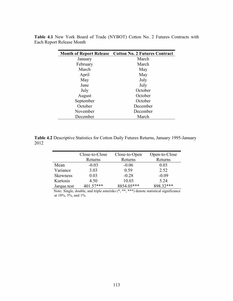
113
Table 4.1 New York Board of Trade (NYBOT) Cotton No. 2 Futures Contracts with Each Report Release Month
Month of Report Release Cotton No. 2 Futures Contract January March February March March May April May May July June July July October
August October September October
October December November December December March
Table 4.2 Descriptive Statistics for Cotton Daily Futures Returns, January 1995-January 2012
Close-to-Close
Returns Close-to-Open
Returns Open-to-Close
Returns Mean -0.03 -0.06 0.03 Variance 3.03 0.59 2.52 Skewness 0.03 -0.28 -0.09 Kurtosis 4.50 10.03 5.24 Jarque.test 401.57*** 8854.05*** 898.32***
Note: Single, double, and triple asterisks (*, **, ***) denote statistical significance at 10%, 5%, and 1%.
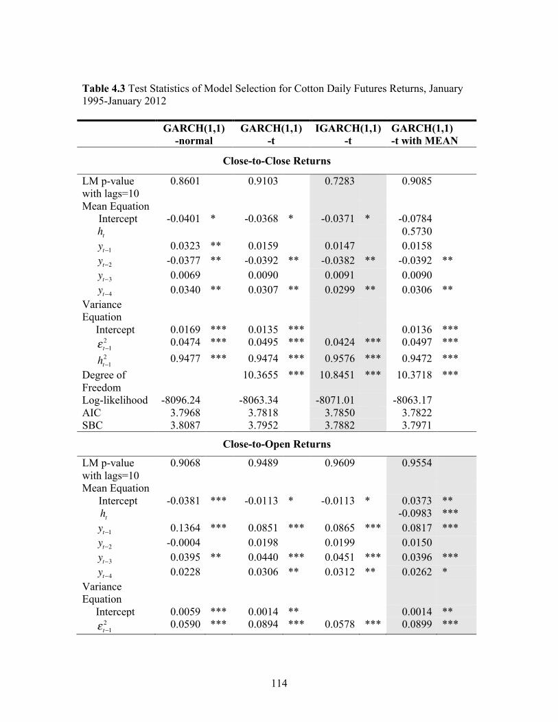
114
Table 4.3 Test Statistics of Model Selection for Cotton Daily Futures Returns, January 1995-January 2012 GARCH(1,1)
-normal GARCH(1,1)
-t IGARCH(1,1)
-t GARCH(1,1) -t with MEAN
Close-to-Close Returns
LM p-value with lags=10
0.8601 0.9103 0.7283 0.9085
Mean Equation Intercept -0.0401 * -0.0368 * -0.0371 * -0.0784 ht 0.5730 0.0323 ** 0.0159 0.0147 0.0158 -0.0377 ** -0.0392 ** -0.0382 ** -0.0392 ** 0.0069 0.0090 0.0091 0.0090 0.0340 ** 0.0307 ** 0.0299 ** 0.0306 ** Variance Equation
Intercept 0.0169 *** 0.0135 *** 0.0136 *** 0.0474 *** 0.0495 *** 0.0424 *** 0.0497 ***
ht−12 0.9477 *** 0.9474 *** 0.9576 *** 0.9472 ***
Degree of Freedom
10.3655 *** 10.8451 *** 10.3718 ***
Log-likelihood -8096.24 -8063.34 -8071.01 -8063.17 AIC 3.7968 3.7818 3.7850 3.7822 SBC 3.8087 3.7952 3.7882 3.7971
Close-to-Open Returns
LM p-value with lags=10
0.9068 0.9489 0.9609 0.9554
Mean Equation Intercept -0.0381 *** -0.0113 * -0.0113 * 0.0373 ** ht -0.0983 *** 0.1364 *** 0.0851 *** 0.0865 *** 0.0817 *** -0.0004 0.0198 0.0199 0.0150 0.0395 ** 0.0440 *** 0.0451 *** 0.0396 *** 0.0228 0.0306 ** 0.0312 ** 0.0262 * Variance Equation
Intercept 0.0059 *** 0.0014 ** 0.0014 ** 0.0590 *** 0.0894 *** 0.0578 *** 0.0899 ***
yt−1yt−2yt−3yt−4
ε t−12
yt−1yt−2yt−3yt−4
ε t−12
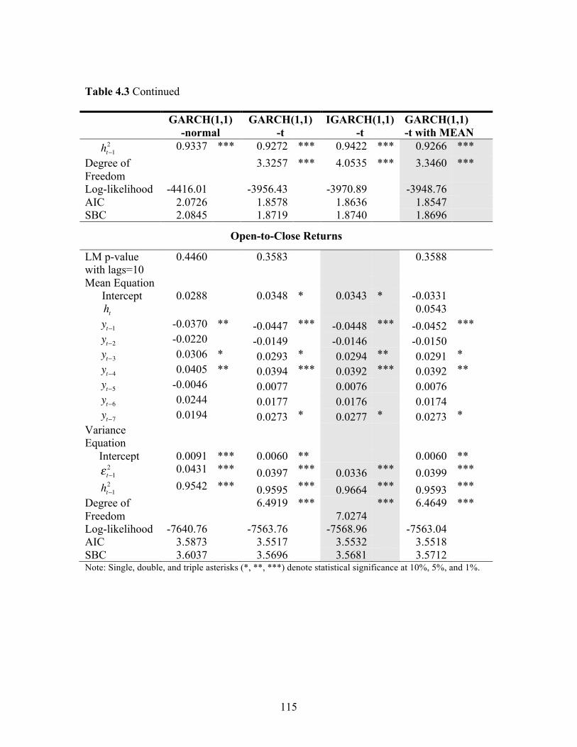
115
Table 4.3 Continued GARCH(1,1)
-normal GARCH(1,1)
-t IGARCH(1,1)
-t GARCH(1,1) -t with MEAN
ht−12 0.9337 *** 0.9272 *** 0.9422 *** 0.9266 ***
Degree of Freedom
3.3257 *** 4.0535 *** 3.3460 ***
Log-likelihood -4416.01 -3956.43 -3970.89 -3948.76 AIC 2.0726 1.8578 1.8636 1.8547 SBC 2.0845 1.8719 1.8740 1.8696
Open-to-Close Returns
LM p-value with lags=10
0.4460 0.3583 0.3588
Mean Equation Intercept 0.0288 0.0348 * 0.0343 * -0.0331 ht 0.0543 -0.0370 ** -0.0447 *** -0.0448 *** -0.0452 *** -0.0220 -0.0149 -0.0146 -0.0150 0.0306 * 0.0293 * 0.0294 ** 0.0291 * 0.0405 ** 0.0394 *** 0.0392 *** 0.0392 ** -0.0046 0.0077 0.0076 0.0076 0.0244 0.0177 0.0176 0.0174 0.0194 0.0273 * 0.0277 * 0.0273 * Variance Equation
Intercept 0.0091 *** 0.0060 ** 0.0060 ** 0.0431 *** 0.0397 *** 0.0336 *** 0.0399 ***
ht−12 0.9542 *** 0.9595 *** 0.9664 *** 0.9593 ***
Degree of Freedom
6.4919 *** 7.0274
*** 6.4649 ***
Log-likelihood -7640.76 -7563.76 -7568.96 -7563.04 AIC 3.5873 3.5517 3.5532 3.5518 SBC 3.6037 3.5696 3.5681 3.5712 Note: Single, double, and triple asterisks (*, **, ***) denote statistical significance at 10%, 5%, and 1%.
yt−1yt−2yt−3yt−4yt−5yt−6yt−7
ε t−12
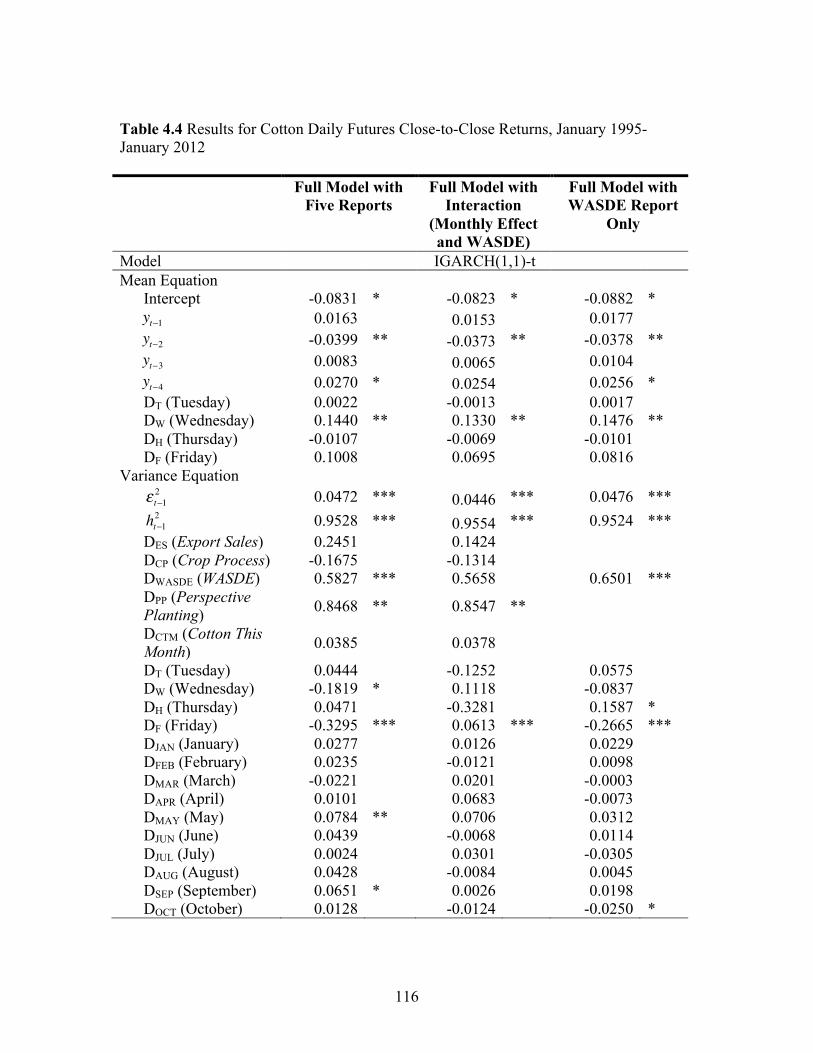
116
Table 4.4 Results for Cotton Daily Futures Close-to-Close Returns, January 1995-January 2012 Full Model with
Five Reports Full Model with
Interaction (Monthly Effect and WASDE)
Full Model with WASDE Report
Only
Model IGARCH(1,1)-t Mean Equation Intercept -0.0831 * -0.0823 * -0.0882 * 0.0163 0.0153 0.0177 -0.0399 ** -0.0373 ** -0.0378 ** 0.0083 0.0065 0.0104 0.0270 * 0.0254 0.0256 * DT (Tuesday) 0.0022 -0.0013 0.0017 DW (Wednesday) 0.1440 ** 0.1330 ** 0.1476 ** DH (Thursday) -0.0107 -0.0069 -0.0101 DF (Friday) 0.1008 0.0695 0.0816 Variance Equation 0.0472 *** 0.0446 *** 0.0476 *** ht−1
2 0.9528 *** 0.9554 *** 0.9524 *** DES (Export Sales) 0.2451 0.1424 DCP (Crop Process) -0.1675 -0.1314 DWASDE (WASDE) 0.5827 *** 0.5658 0.6501 *** DPP (Perspective Planting) 0.8468 ** 0.8547 **
DCTM (Cotton This Month) 0.0385 0.0378
DT (Tuesday) 0.0444 -0.1252 0.0575 DW (Wednesday) -0.1819 * 0.1118 -0.0837 DH (Thursday) 0.0471 -0.3281 0.1587 * DF (Friday) -0.3295 *** 0.0613 *** -0.2665 *** DJAN (January) 0.0277 0.0126 0.0229 DFEB (February) 0.0235 -0.0121 0.0098 DMAR (March) -0.0221 0.0201 -0.0003 DAPR (April) 0.0101 0.0683 -0.0073 DMAY (May) 0.0784 ** 0.0706 0.0312 DJUN (June) 0.0439 -0.0068 0.0114 DJUL (July) 0.0024 0.0301 -0.0305 DAUG (August) 0.0428 -0.0084 0.0045 DSEP (September) 0.0651 * 0.0026 0.0198 DOCT (October) 0.0128 -0.0124 -0.0250 *
yt−1yt−2yt−3yt−4
ε t−12
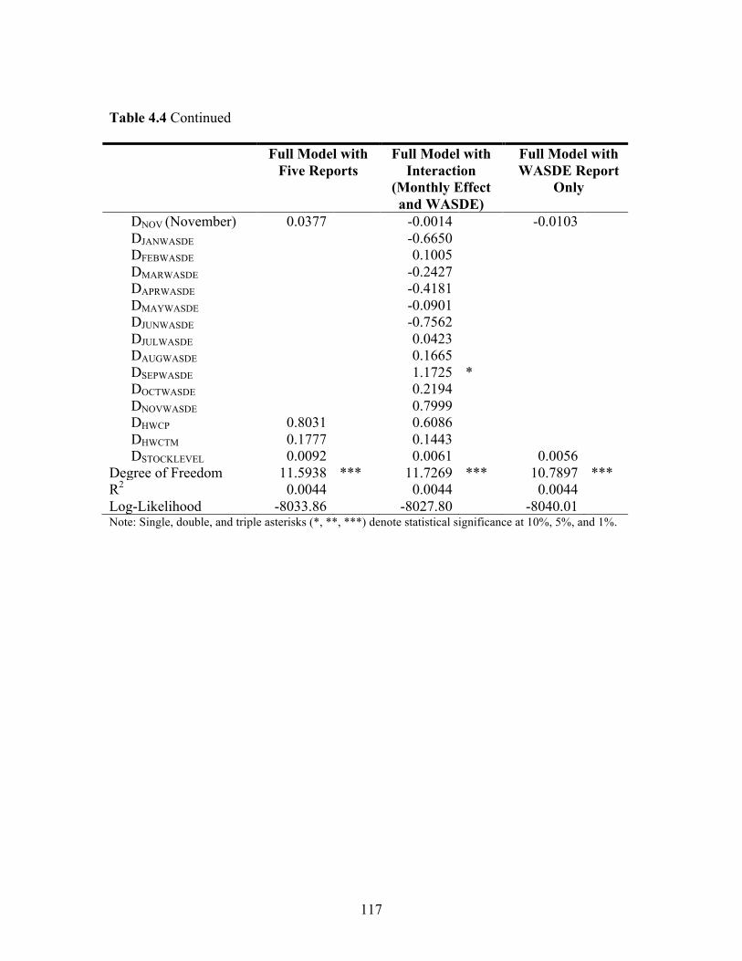
117
Table 4.4 Continued Full Model with
Five Reports Full Model with
Interaction (Monthly Effect and WASDE)
Full Model with WASDE Report
Only
DNOV (November) 0.0377 -0.0014 -0.0103 DJANWASDE -0.6650 DFEBWASDE 0.1005 DMARWASDE -0.2427 DAPRWASDE -0.4181 DMAYWASDE -0.0901 DJUNWASDE -0.7562 DJULWASDE 0.0423 DAUGWASDE 0.1665 DSEPWASDE 1.1725 * DOCTWASDE 0.2194 DNOVWASDE 0.7999 DHWCP 0.8031 0.6086 DHWCTM 0.1777 0.1443 DSTOCKLEVEL 0.0092 0.0061 0.0056 Degree of Freedom 11.5938 *** 11.7269 *** 10.7897 *** R2 0.0044 0.0044 0.0044 Log-Likelihood -8033.86 -8027.80 -8040.01 Note: Single, double, and triple asterisks (*, **, ***) denote statistical significance at 10%, 5%, and 1%.
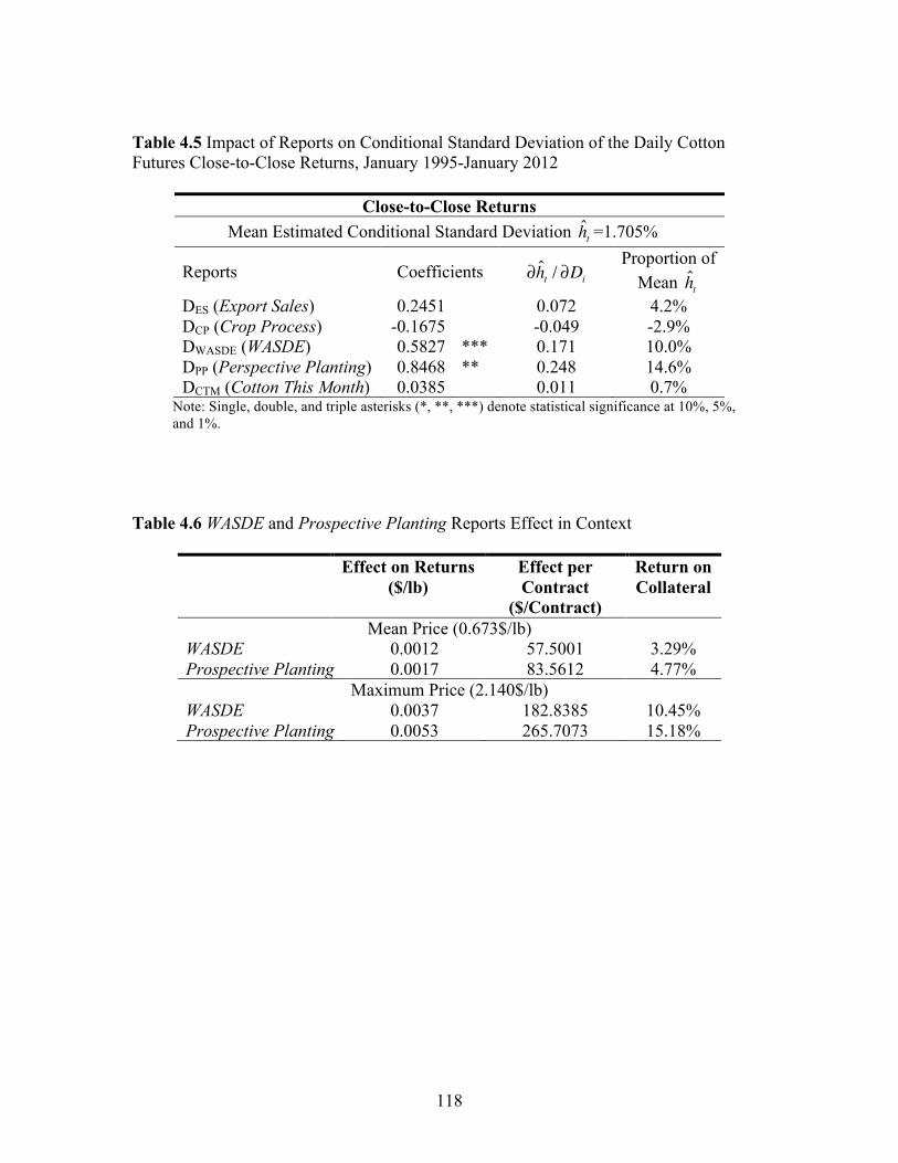
118
Table 4.5 Impact of Reports on Conditional Standard Deviation of the Daily Cotton Futures Close-to-Close Returns, January 1995-January 2012
Close-to-Close Returns Mean Estimated Conditional Standard Deviation ht =1.705%
Reports Coefficients ∂ht / ∂Di Proportion of
Mean ht DES (Export Sales) 0.2451 0.072 4.2% DCP (Crop Process) -0.1675 -0.049 -2.9% DWASDE (WASDE) 0.5827 *** 0.171 10.0% DPP (Perspective Planting) 0.8468 ** 0.248 14.6% DCTM (Cotton This Month) 0.0385 0.011 0.7%
Note: Single, double, and triple asterisks (*, **, ***) denote statistical significance at 10%, 5%, and 1%. Table 4.6 WASDE and Prospective Planting Reports Effect in Context
Effect on Returns ($/lb)
Effect per Contract
($/Contract)
Return on Collateral
Mean Price (0.673$/lb) WASDE 0.0012 57.5001 3.29% Prospective Planting 0.0017 83.5612 4.77%
Maximum Price (2.140$/lb) WASDE 0.0037 182.8385 10.45% Prospective Planting 0.0053 265.7073 15.18%
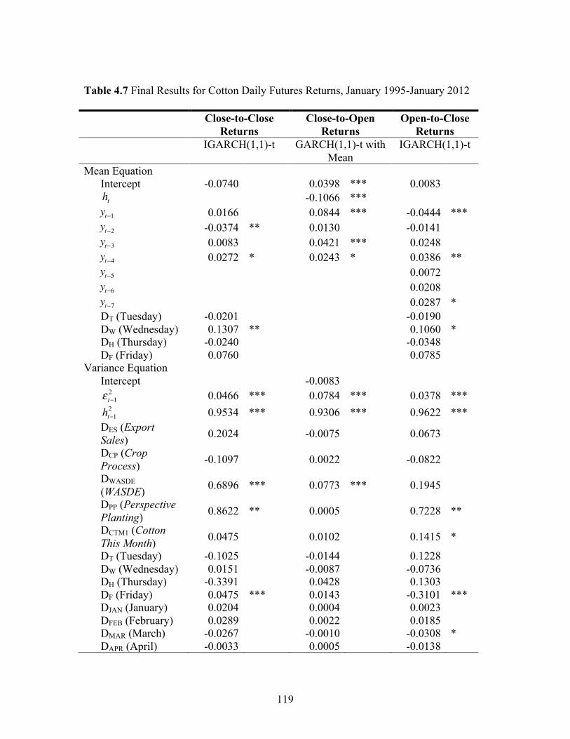
119
Table 4.7 Final Results for Cotton Daily Futures Returns, January 1995-January 2012 Close-to-Close
Returns Close-to-Open
Returns Open-to-Close
Returns IGARCH(1,1)-t GARCH(1,1)-t with
Mean IGARCH(1,1)-t
Mean Equation Intercept -0.0740 0.0398 *** 0.0083 ht -0.1066 *** 0.0166 0.0844 *** -0.0444 *** -0.0374 ** 0.0130 -0.0141 0.0083 0.0421 *** 0.0248 0.0272 * 0.0243 * 0.0386 ** 0.0072 0.0208 0.0287 * DT (Tuesday) -0.0201 -0.0190 DW (Wednesday) 0.1307 ** 0.1060 * DH (Thursday) -0.0240 -0.0348 DF (Friday) 0.0760 0.0785 Variance Equation Intercept -0.0083 0.0466 *** 0.0784 *** 0.0378 *** ht−1
2 0.9534 *** 0.9306 *** 0.9622 *** DES (Export Sales) 0.2024 -0.0075 0.0673
DCP (Crop Process) -0.1097 0.0022 -0.0822
DWASDE (WASDE) 0.6896 *** 0.0773 *** 0.1945
DPP (Perspective Planting) 0.8622 ** 0.0005 0.7228 **
DCTM1 (Cotton This Month) 0.0475 0.0102 0.1415 *
DT (Tuesday) -0.1025 -0.0144 0.1228 DW (Wednesday) 0.0151 -0.0087 -0.0736 DH (Thursday) -0.3391 0.0428 0.1303 DF (Friday) 0.0475 *** 0.0143 -0.3101 *** DJAN (January) 0.0204 0.0004 0.0023 DFEB (February) 0.0289 0.0022 0.0185 DMAR (March) -0.0267 -0.0010 -0.0308 * DAPR (April) -0.0033 0.0005 -0.0138
yt−1yt−2yt−3yt−4yt−5yt−6yt−7
ε t−12
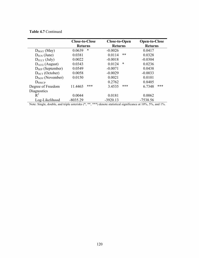
120
Table 4.7 Continued Close-to-Close
Returns Close-to-Open
Returns Open-to-Close
Returns DMAY (May) 0.0639 * -0.0026 0.0417 DJUN (June) 0.0381 0.0114 ** 0.0328 DJULY (July) 0.0022 -0.0018 -0.0304 DAUG (August) 0.0343 0.0124 * 0.0236 DSEP (September) 0.0549 -0.0071 0.0438 DOCT (October) 0.0058 -0.0029 -0.0033 DNOV (November) 0.0150 0.0021 0.0101 DHWCP 0.2762 0.8405 Degree of Freedom 11.4465 *** 3.4535 *** 6.7348 *** Diagnostics R2 0.0044 0.0181 0.0062 Log-Likelihood -8035.29 -3920.13 -7538.56 Note: Single, double, and triple asterisks (*, **, ***) denote statistical significance at 10%, 5%, and 1%.
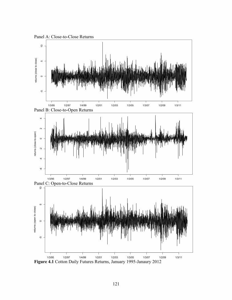
121
-50
510
retu
rns
(clo
se to
clo
se)
1/3/95 1/2/97 1/4/99 1/2/01 1/2/03 1/3/05 1/3/07 1/2/09 1/3/11
Panel A: Close-to-Close Returns Panel B: Close-to-Open Returns
Panel C: Open-to-Close Returns
Figure 4.1 Cotton Daily Futures Returns, January 1995-Janaury 2012
-6-4
-20
24
retu
rns
(clo
se-to
-ope
n)
1/3/95 1/2/97 1/4/99 1/2/01 1/2/03 1/3/05 1/3/07 1/2/09 1/3/11
-50
510
retu
rns
(ope
n to
clo
se)
1/3/95 1/2/97 1/4/99 1/2/01 1/2/03 1/3/05 1/3/07 1/2/09 1/3/11
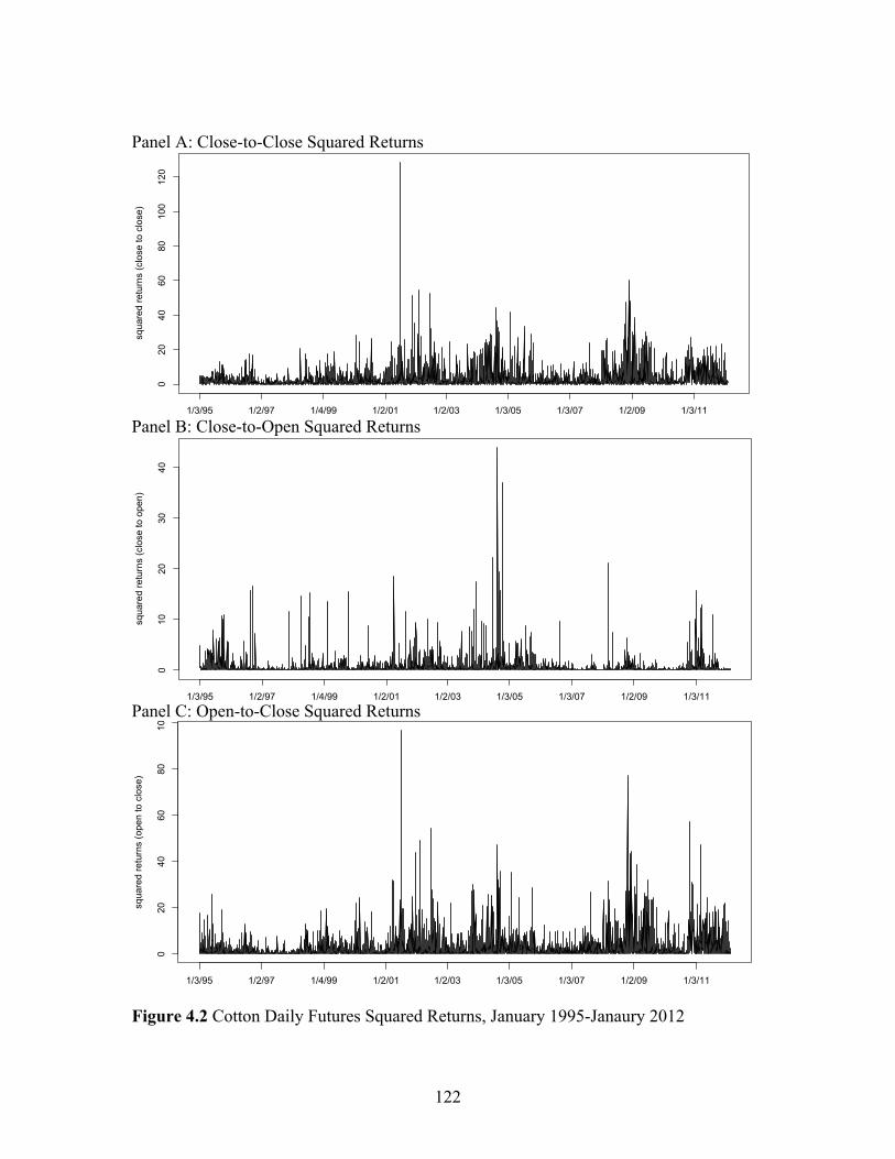
122
Panel A: Close-to-Close Squared Returns
Panel B: Close-to-Open Squared Returns
Panel C: Open-to-Close Squared Returns
Figure 4.2 Cotton Daily Futures Squared Returns, January 1995-Janaury 2012
020
4060
80100
120
squa
red
retu
rns
(clo
se to
clo
se)
1/3/95 1/2/97 1/4/99 1/2/01 1/2/03 1/3/05 1/3/07 1/2/09 1/3/11
010
2030
40
squa
red
retu
rns
(clo
se to
ope
n)
1/3/95 1/2/97 1/4/99 1/2/01 1/2/03 1/3/05 1/3/07 1/2/09 1/3/11
020
4060
80100
squa
red
retu
rns
(ope
n to
clo
se)
1/3/95 1/2/97 1/4/99 1/2/01 1/2/03 1/3/05 1/3/07 1/2/09 1/3/11
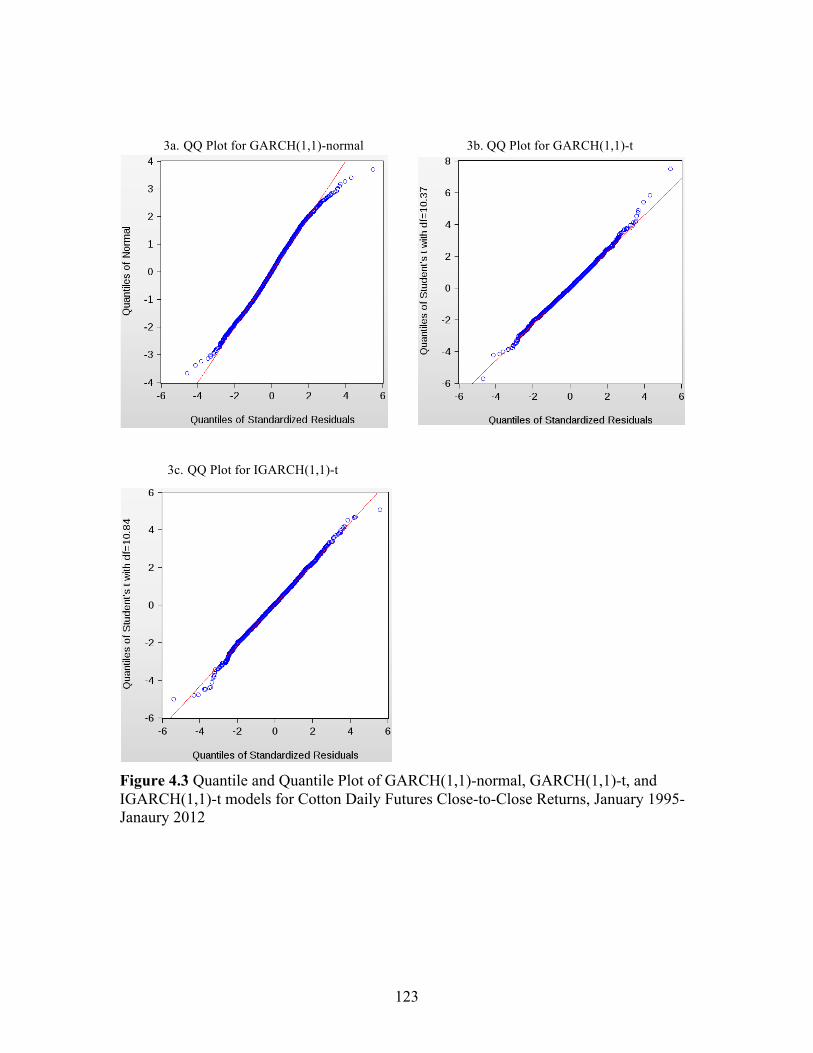
123
3a. QQ Plot for GARCH(1,1)-normal 3b. QQ Plot for GARCH(1,1)-t
3c. QQ Plot for IGARCH(1,1)-t Figure 4.3 Quantile and Quantile Plot of GARCH(1,1)-normal, GARCH(1,1)-t, and IGARCH(1,1)-t models for Cotton Daily Futures Close-to-Close Returns, January 1995-Janaury 2012
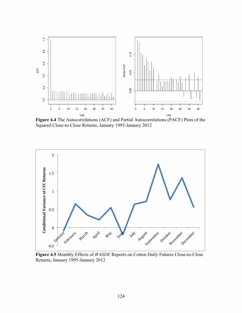
124
Figure 4.4 The Autocorrelations (ACF) and Partial Autocorrelations (PACF) Plots of the Squared Close-to-Close Returns, January 1995-Janaury 2012
Figure 4.5 Monthly Effects of WASDE Reports on Cotton Daily Futures Close-to-Close Returns, January 1995-Janaury 2012
"0.5!
0!
0.5!
1!
1.5!
2!
Conditional)Variance)of)CTC)Returns)
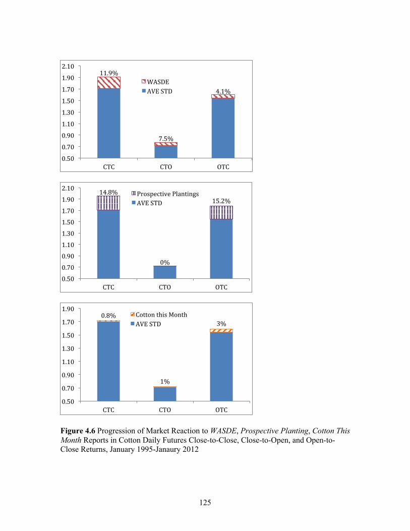
125
Figure 4.6 Progression of Market Reaction to WASDE, Prospective Planting, Cotton This Month Reports in Cotton Daily Futures Close-to-Close, Close-to-Open, and Open-to-Close Returns, January 1995-Janaury 2012
11.9%!
7.5%!
4.1%!
0.50!0.70!0.90!1.10!1.30!1.50!1.70!1.90!2.10!
CTC! CTO! OTC!
WASDE!AVE!STD!
14.8%!
0%!
15.2%!
0.50!0.70!0.90!1.10!1.30!1.50!1.70!1.90!2.10!
CTC! CTO! OTC!
Prospective!Plantings!AVE!STD!
0.8%!
1%!
3%!
0.50!0.70!0.90!1.10!1.30!1.50!1.70!1.90!
CTC! CTO! OTC!
Cotton!this!Month!AVE!STD!
126
CHAPTER FIVE
DISSERTATION SUMMARY
The research implemented statistical tools for examining two economic issues: the
impact of a regional agricultural campaign on participating restaurants and efforts of
USDA forecasting reports in agricultural commodity markets. The first study estimated
the perceived economic value of each of the four components of the Certified South
Carolina campaign from the viewpoint of participating restaurants. A choice experiment
was conducted as part of a restaurant manager survey to estimate average WTP for each
campaign component using a mixed logit model. The four existing campaign components
were treated as attributes in mixed logit model estimation, which also included the
method of payment and the amount of payment for the campaign. Findings indicate that
three existing campaign components--Labeling, Multimedia Advertising, and “Fresh on
the Menu” have a significant positive economic value for restaurants participating in the
program.
This study also shed light on determinants of restaurants’ WTP for the campaign.
We found that restaurants’ image, satisfaction with the campaign, and motivation for
participation significantly affect their WTP for the “Fresh on the Menu”, Signage and
Labeling campaign components. However, restaurants’ size does not affect WTP for any
component. These findings can help the South Carolina Department of Agriculture
marketing the campaign to potential participants.
The second study focused on inefficiency in revisions of WASDE forecasts for
U.S. corn, soybeans, wheat, and cotton. Results from the evaluation of the revision
127
inefficiency showed significant correlations between consecutive forecast revisions in all
crops and all categories except for the seed category in wheat forecasts. Almost
exclusively, inefficiency took the form of smoothing as revisions were positively
correlated. We also discovered that among the forecasts of four crops, smoothing was
most prevalent in soybeans and least common in wheat, and exports was the category
most affected by smoothing.
The widespread evidence of revision inefficiency suggested that forecast accuracy
could be improved if this inefficiency is corrected. Therefore, the second study also
attempted to develop an adjustment procedure that could be used to correct revision
inefficiency and improve the accuracy of these forecasts. New correction procedures for
four commodities were developed as follows: using the OLS estimation for wheat and the
M-estimation for corn, soybeans, and cotton; only considering forecast size and direction
for corn price, soybean beginning stocks, crushings, and price, and wheat production
forecasts. Our findings suggest that the adjustment procedure has the highest potential for
improving accuracy in corn, wheat, and cotton production forecasts.
This third study estimated the impact of all major public and private reports on the
cotton futures market from 1995 through 2012. The estimation was based on the event
study approach with the events measured by the release of 5 major reports: Export Sales,
Crop Progress, WASDE, and Perspective Plantings (public reports from USDA) and
Cotton This Month (private report from ICAC). In measuring the report effects, we
controlled for the day-of-week, seasonality, and stock level effects on cotton futures
returns. A best fitting GARCH-type model was carefully selected to model cotton futures
128
returns, characterized by non-normal, time-varying volatility. Instead of investigating the
information effect of a single report, this study analyzed the impact of five reports
simultaneously, which avoided the issue of overestimation due to “clustering of reports”.
In fact, the results indicated the existence of the “clustering reports” problem as the
coefficient of WASDE report was smaller when we included all 5 reports instead of
having only the WASDE report. Having all five reports also allowed us to judge the
relative impact of different reports. Results indicated the Perspective Planting had the
largest impact in the cotton market, followed by the WASDE reports.
The analysis in the third study was also carried out using the Close-to-Close,
Close-to-Open, and Open-to-Close returns to investigate the progression of market
reaction to new information. This analysis demonstrated that although most of the
reaction to WASDE reports happened immediately after the report release, the cotton
market continuously absorbed the new information throughout the trading day. On the
other hand, the cotton market reacted to the Perspective Planning report not immediately
but slowly during the trading session. Similar results were found in the reaction to the
Cotton This Month report but with a much smaller magnitude.