Embed Size (px)
Citation preview
Application of High Order Traffic Flow Models for Incident
Detection and Modeling Multiclass Flow
Shimao Fan∗ Ren Wang† Daniel B. Work‡
August 25, 2014
Final report submitted to
the University of California, Berkeley
∗Coordinated Science Laboratory, University of Illinois at Urbana Champaign, 205 N. Mathews Ave, Ur-bana, IL 61801 ([email protected])†Department of Civil and Environmental Engineering, University of Illinois at Urbana Champaign, 205 N.
Mathews Ave, Urbana, IL 61801 ([email protected])‡Department of Civil and Environmental Engineering and Coordinated Science Laboratory, University of
Illinois at Urbana Champaign, 205 N. Mathews Ave, Urbana, IL 61801 ([email protected])
1
Abstract
This work is focused on the application of high order traffic flow theory to the problem
of traffic incident detection, and for modeling multiclass traffic flow composed of different
vehicle types.
For incident detection applications, a class of generic second order traffic flow models
(GOSM) is applied to detect traffic incidents in real time by posing the problem as a
hybrid state estimation problem. To incorporate the incident dynamics in the model, a
regime variable is introduced to describe where and how many lanes are blocked during an
incident, resulting in a multiple model framework. This work develops a multiple model
extension to the GOSM on a road network. Then, a discrete version of the GOSM known
as the second order cell transmission model (2CTM) is presented under the framework
of the cell transmission model. Next, this multiple model predictor is integrated with a
particle filter to obtain an estimate of the traffic state and the incident location if it exists.
The proposed algorithm is tested on a road segment in numerical simulation using the
CORSIM traffic microsimulation software as the true state.
In the second application, a new family of high order traffic flow models is considered
as an extension to the scalar Lighthill Whitham Richards (LWR) model. Under this
framework, a heterogeneous traffic model with two vehicle classes is developed to capture
an important phenomenon in highly heterogeneous traffic flows called creeping. Creeping
occurs when small vehicles such as motorcycles continue to advance in congestion even
though larger vehicles have completely stopped, for example via lane sharing. The new
model is a phase transition model which applies a system of conservation laws in the non-
creeping phase, and a scalar model in the creeping phase. The solution to the Riemann
problem is obtained by investigating the elementary waves, in particular for the cases
when one vehicle class is absent, as well as in the presence of a phase transition. Based
on the proposed Riemann solver, the solution to the Cauchy problem is constructed using
wavefront tracking. Numerical tests are carried out using a Godunov scheme to illustrate
the creeping phenomenon.
2
Contents
1 Introduction 7
1.1 Real Time Incident Detection . . . . . . . . . . . . . . . . . . . . . . . . . . . 7
1.2 Heterogeneous Multiclass Traffic Modeling . . . . . . . . . . . . . . . . . . . . 8
1.3 Contributions and Outline . . . . . . . . . . . . . . . . . . . . . . . . . . . . 9
2 Joint Traffic State Estimation and Incident Detection 10
2.1 Second Order Traffic Model . . . . . . . . . . . . . . . . . . . . . . . . . . . . 11
2.1.1 Generic Framework of Second Order Models . . . . . . . . . . . . . . . 11
2.1.2 Classification of the GOSM . . . . . . . . . . . . . . . . . . . . . . . . 12
2.2 Multiple Model Second Order Cell Transmission Model . . . . . . . . . . . . . 15
2.2.1 Cell Transmission Model . . . . . . . . . . . . . . . . . . . . . . . . . . 16
2.2.2 Second Order Cell Transmission Model . . . . . . . . . . . . . . . . . . 17
2.2.3 Sending and Receiving Functions of 2CTM . . . . . . . . . . . . . . . 19
2.2.4 Intermediate Traffic State . . . . . . . . . . . . . . . . . . . . . . . . . 20
2.2.5 A Multiple Model Framework for 2CTM . . . . . . . . . . . . . . . . . 23
2.3 A Multiple Model 2CTM on Road Network . . . . . . . . . . . . . . . . . . . 24
2.3.1 Bottleneck: One Incoming Link and One Outgoing Link . . . . . . . . 26
2.3.2 Diverge: One Incoming Link and Two Outgoing Links . . . . . . . . . 30
2.3.3 Merge: Two Incoming Links and One Outgoing Link . . . . . . . . . . 33
2.3.4 A Multiple Model Framework on a Road Network . . . . . . . . . . . 36
2.4 A Hybrid State Estimation Problem . . . . . . . . . . . . . . . . . . . . . . . 36
2.5 Simulation Results Based on CORSIM . . . . . . . . . . . . . . . . . . . . . . 41
3 Heterogeneous Traffic Flow Model with Creeping 47
3
3.1 Classification of Multiclass Traffic Models . . . . . . . . . . . . . . . . . . . . 47
3.1.1 Homogeneous Multiclass Models . . . . . . . . . . . . . . . . . . . . . 47
3.1.2 Heterogeneous Multiclass Models . . . . . . . . . . . . . . . . . . . . . 49
3.2 Interpretation of the GOSM as a Two Class Homogeneous Multiclass Model . 50
3.3 A New Heterogeneous Model with Creeping . . . . . . . . . . . . . . . . . . . 52
3.4 Model Analysis . . . . . . . . . . . . . . . . . . . . . . . . . . . . . . . . . . . 55
3.4.1 Hyperbolicity of the Creeping Model in D1 . . . . . . . . . . . . . . . 56
3.4.2 Property of the Characteristic Fields . . . . . . . . . . . . . . . . . . . 58
3.4.3 Elementary Waves . . . . . . . . . . . . . . . . . . . . . . . . . . . . . 60
3.4.4 Riemann Solver in D . . . . . . . . . . . . . . . . . . . . . . . . . . . . 64
3.4.5 Invariance of D . . . . . . . . . . . . . . . . . . . . . . . . . . . . . . . 66
3.4.6 Cauchy Problem . . . . . . . . . . . . . . . . . . . . . . . . . . . . . . 67
3.4.7 Vacuum Problem . . . . . . . . . . . . . . . . . . . . . . . . . . . . . . 67
3.5 Numerical Simulations . . . . . . . . . . . . . . . . . . . . . . . . . . . . . . . 71
3.5.1 Numerical Method . . . . . . . . . . . . . . . . . . . . . . . . . . . . . 71
3.5.2 Numerical Simulations and Comparisons . . . . . . . . . . . . . . . . . 73
4 Conclusion 77
4
List of Tables
1 Classification of multiclass models according to the definition of velocity functions. 48
List of Figures
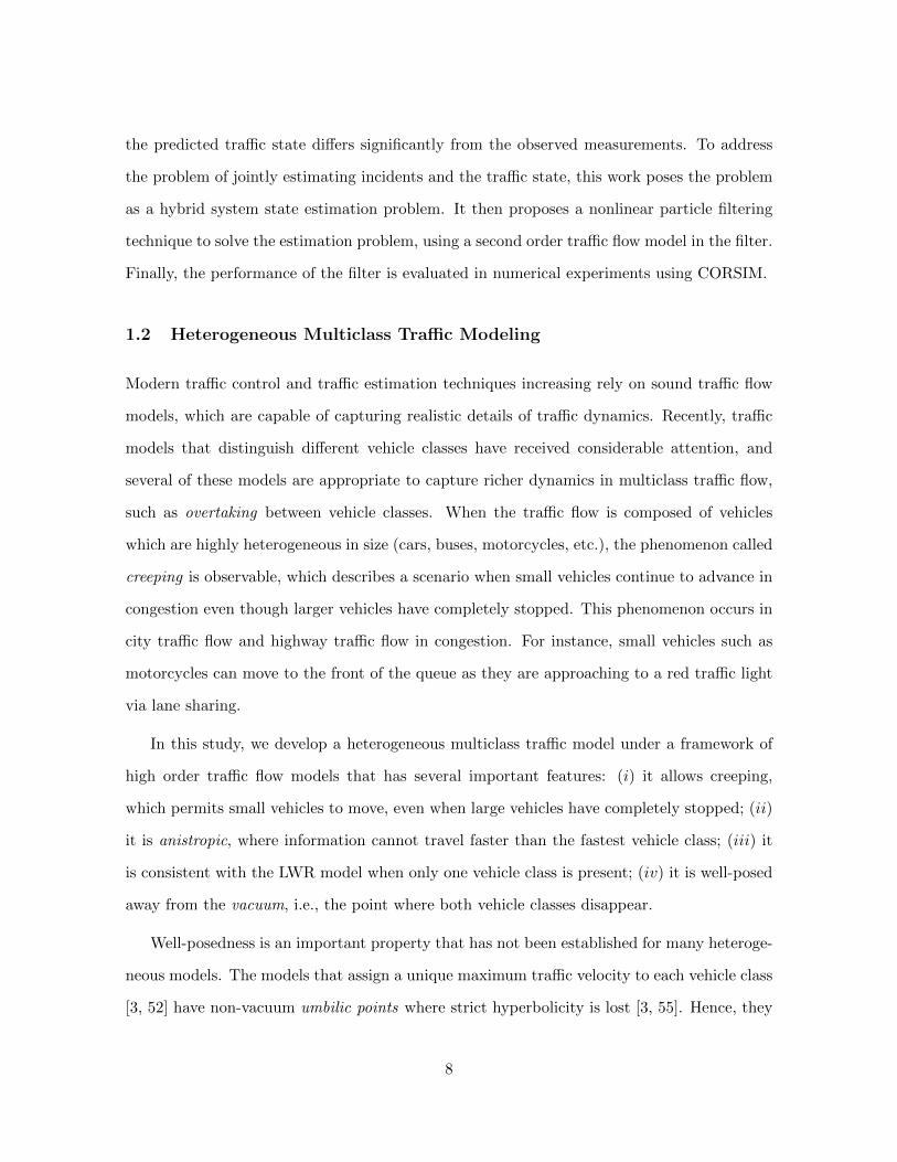
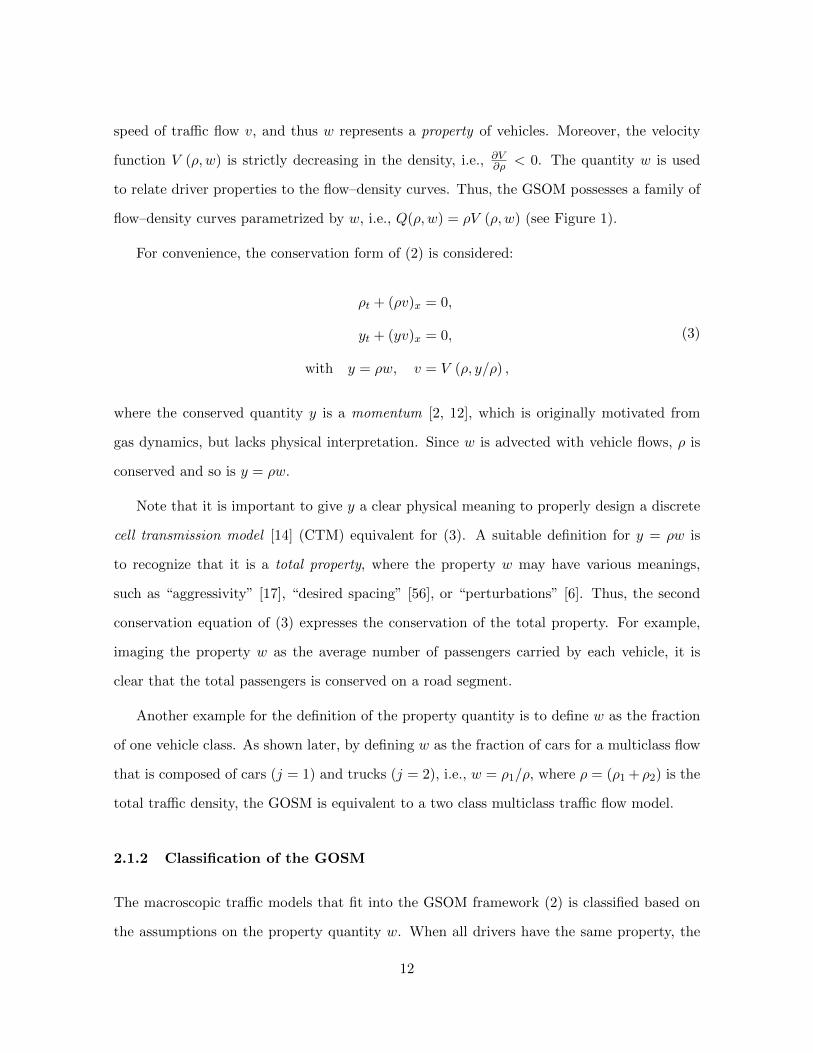
1 (a) flow–density curves of the GARZ model [17]. (b) flow–density curves of a
phase transition model. (c) illustrates the idea of collapsed model [18]. . . . . 13
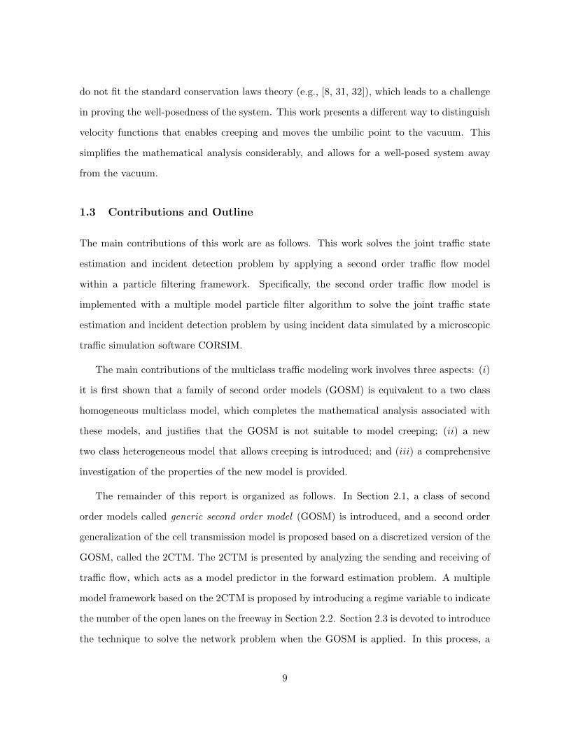
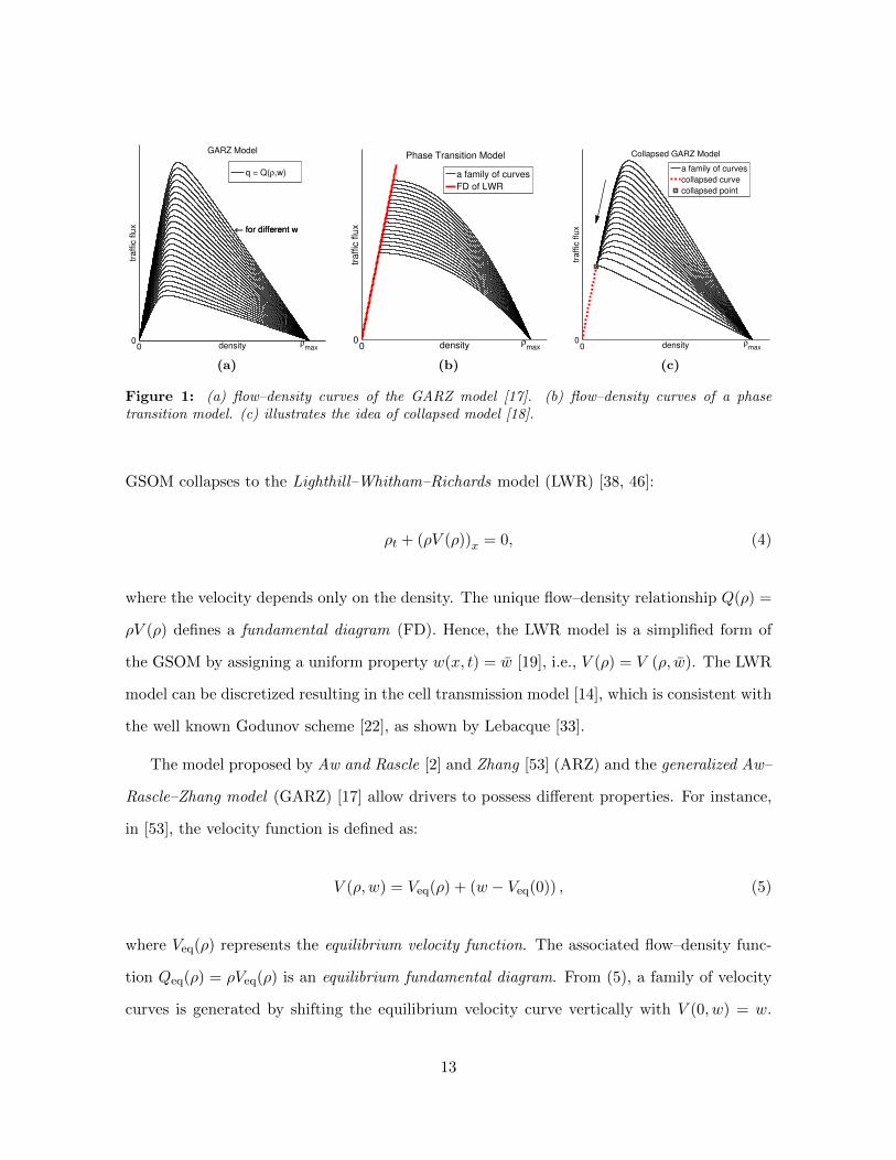
2 The cell transmission model. . . . . . . . . . . . . . . . . . . . . . . . . . . . . 15
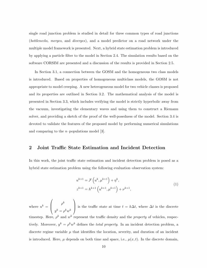
3 Second order cell transmission model. . . . . . . . . . . . . . . . . . . . . . . . 17
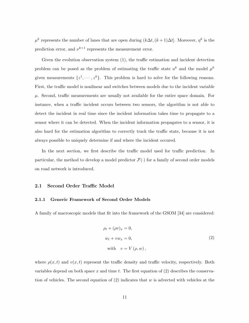
4 (a) is the sending function and (b) is the receiving function of the 2CTM based
on the CGARZ model [18], illustrated for the case where wL > wR. . . . . . . 18
5 (a): upstream vehicles have the potential to match the downstream velocity,
i.e., vR ≤ V (0, wL) or vR ≤ Q′(0, wL), in which case vM = vR and (b): the
maximum possible velocity of upstream vehicles is lower than the downstream
velocity, i.e., vR > V (0, wL) or vR > Q′(0, wL). In this case, let vM = V (0, wL)
in order to minimize the gap to the downstream velocity. . . . . . . . . . . . . 22
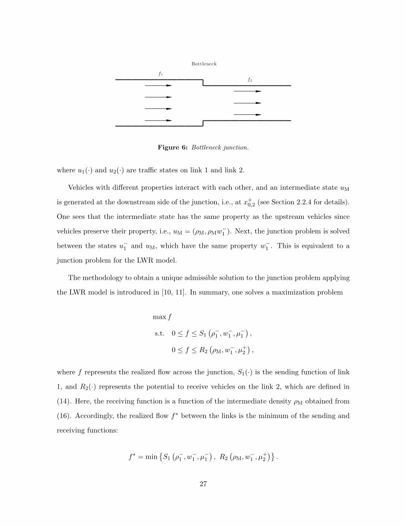
6 Bottleneck junction. . . . . . . . . . . . . . . . . . . . . . . . . . . . . . . . . 27
7 (a) is a diverge junction, and (b) is a merge junction. . . . . . . . . . . . . . 29
8 Maximization problem for diverge junction. Here, three cases (a), (b), (c)
illustrate different selections of priority rule. The points P that are marked
blue–star represent the solutions which maximize the inflow or outflow. . . . . 31
9 True evolution of the traffic density and the model variable. . . . . . . . . . . 42
10 Calibrated fundamental diagrm for the second order traffic flow model. . . . . 44
11 Estimation results of the MMPF, probe vehicle headway 10 seconds (first row),
probe vehicle headway 20 seconds (second row), probe vehicle headway 20 sec-
onds (third row). . . . . . . . . . . . . . . . . . . . . . . . . . . . . . . . . . . 45
5
12 Estimated density error, probe vehicle headway 10 seconds (left), probe vehicle
headway 20 seconds (center), probe vehicle headway 40 seconds (right). . . . . 46
13 probe vehicle headway 10 seconds, estimated density (left), and estimation error
(right). . . . . . . . . . . . . . . . . . . . . . . . . . . . . . . . . . . . . . . . . 46
14 (a) Velocity functions of the creeping model (51). Here, the solid-gray line
represents the velocity of the first vehicle class, and the dashed-blue line is the
velocity of the second vehicle class. (b) The domain of the creeping model (51). 53
15 Lax shock curves starting at u0 ∈ D1. (a) illustrates the case when u0 is interior
of D1. (b) shows the case with u0 on the ρ2-axis. (c) corresponds to the case
with u0 on the ρ1-axis. In (a), the curves with r > ρ01 + ρ0
2 are marked as red,
and those with r < ρ01 + ρ0
2 are in blue color. In (b) and (c), 1–shock curves
(squared-gray) remain in D3, and 2–shock curves (solid-red) are convex and
monotonic. . . . . . . . . . . . . . . . . . . . . . . . . . . . . . . . . . . . . . 61
16 Example 1: an experiment of overtaking. (a) exhibits the traffic state of the
n–populations model at t = 50; (b) shows the numerical results of the creeping
model at t = 33. In each figure, the densities of the first vehicle class (thick-
solid-gray) and the second vehicle class (thick-dashed-black), together with the
initial condition (thin-dashed-red) are shown. . . . . . . . . . . . . . . . . . . 74
17 Example 2: an experiment of creeping. (a) and (c) (left panel) are the simu-
lation results of the n–populations model at t = 33 and t = 150, respectively.
(b) and (d) (right panel) exhibit the results of the creeping model at t = 33 and
t = 150, respectively. . . . . . . . . . . . . . . . . . . . . . . . . . . . . . . . . 75
6
1 Introduction
This work is focused on solving the following two research problems. The first objective is to
develop a multiple model traffic state estimation framework based on a family of second order
traffic flow models and apply it to detect traffic incidents in real time. The second objective
is to design a new model for multiclass traffic flow that can capture several key features of
the flow when vehicles are heterogeneous in size.
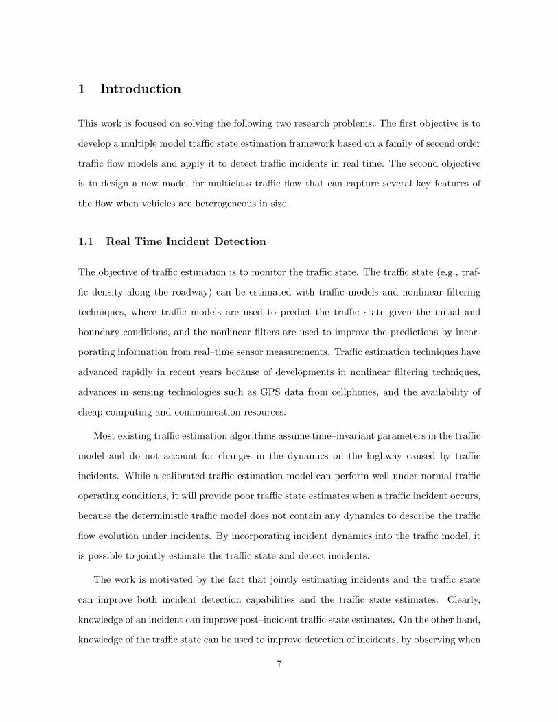
1.1 Real Time Incident Detection
The objective of traffic estimation is to monitor the traffic state. The traffic state (e.g., traf-
fic density along the roadway) can be estimated with traffic models and nonlinear filtering
techniques, where traffic models are used to predict the traffic state given the initial and
boundary conditions, and the nonlinear filters are used to improve the predictions by incor-
porating information from real–time sensor measurements. Traffic estimation techniques have
advanced rapidly in recent years because of developments in nonlinear filtering techniques,
advances in sensing technologies such as GPS data from cellphones, and the availability of
cheap computing and communication resources.
Most existing traffic estimation algorithms assume time–invariant parameters in the traffic
model and do not account for changes in the dynamics on the highway caused by traffic
incidents. While a calibrated traffic estimation model can perform well under normal traffic
operating conditions, it will provide poor traffic state estimates when a traffic incident occurs,
because the deterministic traffic model does not contain any dynamics to describe the traffic
flow evolution under incidents. By incorporating incident dynamics into the traffic model, it
is possible to jointly estimate the traffic state and detect incidents.
The work is motivated by the fact that jointly estimating incidents and the traffic state
can improve both incident detection capabilities and the traffic state estimates. Clearly,
knowledge of an incident can improve post–incident traffic state estimates. On the other hand,
knowledge of the traffic state can be used to improve detection of incidents, by observing when
7
the predicted traffic state differs significantly from the observed measurements. To address
the problem of jointly estimating incidents and the traffic state, this work poses the problem
as a hybrid system state estimation problem. It then proposes a nonlinear particle filtering
technique to solve the estimation problem, using a second order traffic flow model in the filter.
Finally, the performance of the filter is evaluated in numerical experiments using CORSIM.
1.2 Heterogeneous Multiclass Traffic Modeling
Modern traffic control and traffic estimation techniques increasing rely on sound traffic flow
models, which are capable of capturing realistic details of traffic dynamics. Recently, traffic
models that distinguish different vehicle classes have received considerable attention, and
several of these models are appropriate to capture richer dynamics in multiclass traffic flow,
such as overtaking between vehicle classes. When the traffic flow is composed of vehicles
which are highly heterogeneous in size (cars, buses, motorcycles, etc.), the phenomenon called
creeping is observable, which describes a scenario when small vehicles continue to advance in
congestion even though larger vehicles have completely stopped. This phenomenon occurs in
city traffic flow and highway traffic flow in congestion. For instance, small vehicles such as
motorcycles can move to the front of the queue as they are approaching to a red traffic light
via lane sharing.
In this study, we develop a heterogeneous multiclass traffic model under a framework of
high order traffic flow models that has several important features: (i) it allows creeping,
which permits small vehicles to move, even when large vehicles have completely stopped; (ii)
it is anistropic, where information cannot travel faster than the fastest vehicle class; (iii) it
is consistent with the LWR model when only one vehicle class is present; (iv) it is well-posed
away from the vacuum, i.e., the point where both vehicle classes disappear.
Well-posedness is an important property that has not been established for many heteroge-
neous models. The models that assign a unique maximum traffic velocity to each vehicle class
[3, 52] have non-vacuum umbilic points where strict hyperbolicity is lost [3, 55]. Hence, they
8
do not fit the standard conservation laws theory (e.g., [8, 31, 32]), which leads to a challenge
in proving the well-posedness of the system. This work presents a different way to distinguish
velocity functions that enables creeping and moves the umbilic point to the vacuum. This
simplifies the mathematical analysis considerably, and allows for a well-posed system away
from the vacuum.
1.3 Contributions and Outline
The main contributions of this work are as follows. This work solves the joint traffic state
estimation and incident detection problem by applying a second order traffic flow model
within a particle filtering framework. Specifically, the second order traffic flow model is
implemented with a multiple model particle filter algorithm to solve the joint traffic state
estimation and incident detection problem by using incident data simulated by a microscopic
traffic simulation software CORSIM.
The main contributions of the multiclass traffic modeling work involves three aspects: (i)
it is first shown that a family of second order models (GOSM) is equivalent to a two class
homogeneous multiclass model, which completes the mathematical analysis associated with
these models, and justifies that the GOSM is not suitable to model creeping; (ii) a new
two class heterogeneous model that allows creeping is introduced; and (iii) a comprehensive
investigation of the properties of the new model is provided.
The remainder of this report is organized as follows. In Section 2.1, a class of second
order models called generic second order model (GOSM) is introduced, and a second order
generalization of the cell transmission model is proposed based on a discretized version of the
GOSM, called the 2CTM. The 2CTM is presented by analyzing the sending and receiving of
traffic flow, which acts as a model predictor in the forward estimation problem. A multiple
model framework based on the 2CTM is proposed by introducing a regime variable to indicate
the number of the open lanes on the freeway in Section 2.2. Section 2.3 is devoted to introduce
the technique to solve the network problem when the GOSM is applied. In this process, a
9
single road junction problem is studied in detail for three common types of road junctions
(bottlenecks, merges, and diverges), and a model predictor on a road network under the
multiple model framework is presented. Next, a hybrid state estimation problem is introduced
by applying a particle filter to the model in Section 2.4. The simulation results based on the
software CORSIM are presented and a discussion of the results is provided in Section 2.5.
In Section 3.1, a connection between the GOSM and the homogeneous two class models
is introduced. Based on properties of homogeneous multiclass models, the GOSM is not
appropriate to model creeping. A new heterogeneous model for two vehicle classes is proposed
and its properties are outlined in Section 3.2. The mathematical analysis of the model is
presented in Section 3.3, which includes verifying the model is strictly hyperbolic away from
the vacuum, investigating the elementary waves and using them to construct a Riemann
solver, and providing a sketch of the proof of the well-posedness of the model. Section 3.4 is
devoted to validate the features of the proposed model by performing numerical simulations
and comparing to the n–populations model [3].
2 Joint Traffic State Estimation and Incident Detection
In this work, the joint traffic state estimation and incident detection problem is posed as a
hybrid state estimation problem using the following evaluation–observation system:
uk+1 = F(uk, µk+1
)+ ηk,
zk+1 = hk+1(uk+1, µk+1
)+ νk+1,
(1)
where uk =
ρk
yk = ρkwk
is the traffic state at time t = k∆t, where ∆t is the discrete
timestep. Here, ρk and wk represent the traffic density and the property of vehicles, respec-
tively. Moreover, yk = ρkwk defines the total property. In an incident detection problem, a
discrete regime variable µ that identifies the location, severity, and duration of an incident
is introduced. Here, µ depends on both time and space, i.e., µ(x, t). In the discrete domain,
10
µk represents the number of lanes that are open during (k∆t, (k+ 1)∆t]. Moreover, ηk is the
prediction error, and νk+1 represents the measurement error.
Given the evolution observation system (1), the traffic estimation and incident detection
problem can be posed as the problem of estimating the traffic state uk and the model µk
given measurements z1, · · · , zk. This problem is hard to solve for the following reasons.
First, the traffic model is nonlinear and switches between models due to the incident variable
µ. Second, traffic measurements are usually not available for the entire space domain. For
instance, when a traffic incident occurs between two sensors, the algorithm is not able to
detect the incident in real time since the incident information takes time to propagate to a
sensor where it can be detected. When the incident information propagates to a sensor, it is
also hard for the estimation algorithm to correctly track the traffic state, because it is not
always possible to uniquely determine if and where the incident occured.
In the next section, we first describe the traffic model used for traffic prediction. In
particular, the method to develop a model predictor F(·) for a family of second order models
on road network is introduced.
2.1 Second Order Traffic Model
2.1.1 Generic Framework of Second Order Models
A family of macroscopic models that fit into the framework of the GSOM [34] are considered:
ρt + (ρv)x = 0,
wt + vwx = 0,
with v = V (ρ, w) ,
(2)
where ρ(x, t) and v(x, t) represent the traffic density and traffic velocity, respectively. Both
variables depend on both space x and time t. The first equation of (2) describes the conserva-
tion of vehicles. The second equation of (2) indicates that w is advected with vehicles at the
11
speed of traffic flow v, and thus w represents a property of vehicles. Moreover, the velocity
function V (ρ, w) is strictly decreasing in the density, i.e., ∂V∂ρ < 0. The quantity w is used
to relate driver properties to the flow–density curves. Thus, the GSOM possesses a family of
flow–density curves parametrized by w, i.e., Q(ρ, w) = ρV (ρ, w) (see Figure 1).
For convenience, the conservation form of (2) is considered:
ρt + (ρv)x = 0,
yt + (yv)x = 0,
with y = ρw, v = V (ρ, y/ρ) ,
(3)
where the conserved quantity y is a momentum [2, 12], which is originally motivated from
gas dynamics, but lacks physical interpretation. Since w is advected with vehicle flows, ρ is
conserved and so is y = ρw.
Note that it is important to give y a clear physical meaning to properly design a discrete
cell transmission model [14] (CTM) equivalent for (3). A suitable definition for y = ρw is
to recognize that it is a total property, where the property w may have various meanings,
such as “aggressivity” [17], “desired spacing” [56], or “perturbations” [6]. Thus, the second
conservation equation of (3) expresses the conservation of the total property. For example,
imaging the property w as the average number of passengers carried by each vehicle, it is
clear that the total passengers is conserved on a road segment.
Another example for the definition of the property quantity is to define w as the fraction
of one vehicle class. As shown later, by defining w as the fraction of cars for a multiclass flow
that is composed of cars (j = 1) and trucks (j = 2), i.e., w = ρ1/ρ, where ρ = (ρ1 + ρ2) is the
total traffic density, the GOSM is equivalent to a two class multiclass traffic flow model.
2.1.2 Classification of the GOSM
The macroscopic traffic models that fit into the GSOM framework (2) is classified based on
the assumptions on the property quantity w. When all drivers have the same property, the
12
GARZ Model
density
traffic
flu
x
0 ρmax
0
← for different w ← for different w
q = Q(ρ,w)
(a)
Phase Transition Model
densitytr
aff
ic f
lux
0 ρmax
0
a family of curves
FD of LWR
(b)
Collapsed GARZ Model
density
tra
ffic
flu
x
0 ρmax
0
a family of curves
collapsed curve
collapsed point
(c)
Figure 1: (a) flow–density curves of the GARZ model [17]. (b) flow–density curves of a phasetransition model. (c) illustrates the idea of collapsed model [18].
GSOM collapses to the Lighthill–Whitham–Richards model (LWR) [38, 46]:
ρt + (ρV (ρ))x = 0, (4)
where the velocity depends only on the density. The unique flow–density relationship Q(ρ) =
ρV (ρ) defines a fundamental diagram (FD). Hence, the LWR model is a simplified form of
the GSOM by assigning a uniform property w(x, t) = w [19], i.e., V (ρ) = V (ρ, w). The LWR
model can be discretized resulting in the cell transmission model [14], which is consistent with
the well known Godunov scheme [22], as shown by Lebacque [33].
The model proposed by Aw and Rascle [2] and Zhang [53] (ARZ) and the generalized Aw–
Rascle–Zhang model (GARZ) [17] allow drivers to possess different properties. For instance,
in [53], the velocity function is defined as:
V (ρ, w) = Veq(ρ) + (w − Veq(0)) , (5)
where Veq(ρ) represents the equilibrium velocity function. The associated flow–density func-
tion Qeq(ρ) = ρVeq(ρ) is an equilibrium fundamental diagram. From (5), a family of velocity
curves is generated by shifting the equilibrium velocity curve vertically with V (0, w) = w.
13
One sees that ∂V∂w = 1 > 0, which means that the traffic velocity always depends on w for
ρ ∈ [0, ρmax], where ρmax is the maximum traffic density. Similarly, one also has ∂V∂w > 0 for
ρ ∈ [0, ρmax] in the GARZ model. As a result, the flow–density curves of the ARZ and GARZ
models are distinct even in freeflow (away from the vacuum, i.e., ρ = 0), (see Figure 1(a)).
Thus, these models are not appropriate to capture distinct behaviors in the freeflow and
congested regimes based on empirical observation by Kerner [28, 29], who observed that the
experimental flow data is positively proportional to the density data in freeflow, while the
flow–density data exhibits large spread in congestion.
For the collapsed generalized ARZ model (CGARZ) [18], it is assumed that the difference
in property does not affect the traffic velocity in freeflow. This means that vehicles always
possess different properties, but the traffic velocity is not affected by w in freeflow, i.e.,
∂V∂w = 0. The CGARZ model is a special form of the GARZ model that collapses the flow–
density curves into a single curve in the freeflow region (see Figure 1(c)). As a result, all the
analytical results of the ARZ and the GARZ models [2, 17, 34] transfer over to the CGARZ
model. Furthermore, the CGARZ model successfully captures distinct behaviors of traffic
flow in the freeflow and congested regions.
Based on the assumption on w, one sees an important distinction between phase transition
models [5, 6, 12, 13] and the GOSM. In phase transition models, an LWR model is applied in
the freeflow phase Ωf, and a second order model is employed in the congested phase Ωc (see
Figure 1(b)). Hence, phase transition models assume a uniform property w in Ωf, but allow
for different properties in Ωc. These models admit phase transitions in traffic flow, which
agrees with Kerner’s empirical observation [28, 29]. However, by fixing w in freeflow, a phase
transition model uses the philosophy that vehicles lose their properties in Ωf. In contrast, the
GOSM assumes that drivers always preserve their properties, independent of the congestion
level.
One sees that the CGARZ model [18] combines the good features of both phase transition
models [5, 6, 12, 13] and the GARZ model [17], while it also avoids the complicated analytical
work in a phase transition model. It is also appropriate to model distinct behaviors in freeflow
14
ρkj−1 ρ
kj ρ
kj+1
→
→
→
→
→
→
F kj−1/2 F k
j+1/2
j − 1 j − 1/2 j j + 1/2 j + 1
Figure 2: The cell transmission model.
and congested phases based on Kerner’s theory [28, 29]. For the simulations performed in
this study, the CGARZ model is applied. Next, a discrete formulation of the GOSM (3) is
developed under the CTM framework.
2.2 Multiple Model Second Order Cell Transmission Model
The multiple model framework is based on the fact that traffic model changes in the presence
of an incident. In this section, a second order cell transmission model (2CTM) without an
incident is presented first. Then, a multiple model framework based on the 2CTM is developed
by involving the regime variable µ, which denotes the number of lanes that is open.
Mostly due to the complexity of the mathematical analysis, and the difficulty to obtain
physical interpretations in the construction of solutions for the GOSM (3) (e.g., the existence
of an intermediate state in the Riemann solver [2, 12]), it is desirable to reformulate the
GOSM (3) in a more intuitive way such as the CTM. In [35], a Riemann solver to the GOSM
is constructed by examining the sending and receiving functions for traffic, which is consistent
with the original solver that is based on analyzing elementary waves (see e.g., [2, 53]). This
equivalence makes it possible to construct the 2CTM by analyzing the potential to send
vehicles from the upstream cell and receive vehicles from the downstream cell.
15
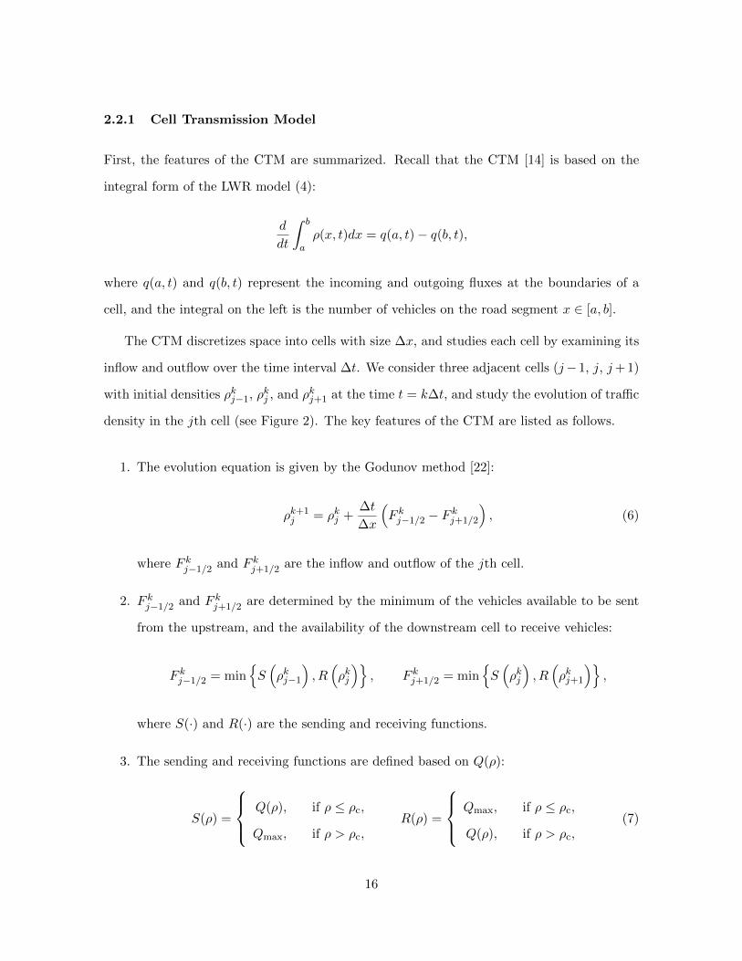
2.2.1 Cell Transmission Model
First, the features of the CTM are summarized. Recall that the CTM [14] is based on the
integral form of the LWR model (4):
d
dt
∫ b
aρ(x, t)dx = q(a, t)− q(b, t),
where q(a, t) and q(b, t) represent the incoming and outgoing fluxes at the boundaries of a
cell, and the integral on the left is the number of vehicles on the road segment x ∈ [a, b].
The CTM discretizes space into cells with size ∆x, and studies each cell by examining its
inflow and outflow over the time interval ∆t. We consider three adjacent cells (j−1, j, j+ 1)
with initial densities ρkj−1, ρkj , and ρkj+1 at the time t = k∆t, and study the evolution of traffic
density in the jth cell (see Figure 2). The key features of the CTM are listed as follows.
1. The evolution equation is given by the Godunov method [22]:
ρk+1j = ρkj +
∆t
∆x
(F kj−1/2 − F
kj+1/2
), (6)
where F kj−1/2 and F kj+1/2 are the inflow and outflow of the jth cell.
2. F kj−1/2 and F kj+1/2 are determined by the minimum of the vehicles available to be sent
from the upstream, and the availability of the downstream cell to receive vehicles:
F kj−1/2 = minS(ρkj−1
), R(ρkj
), F kj+1/2 = min
S(ρkj
), R(ρkj+1
),
where S(·) and R(·) are the sending and receiving functions.
3. The sending and receiving functions are defined based on Q(ρ):
S(ρ) =
Q(ρ), if ρ ≤ ρc,
Qmax, if ρ > ρc,R(ρ) =
Qmax, if ρ ≤ ρc,
Q(ρ), if ρ > ρc,(7)
16
(
ρkj−1
ykj−1
) (
ρkj
ykj
) (
ρkj+1
ykj+1
)
→
→
→
→
→
→
F ρ
j−1/2
F yj−1/2
F ρ
j+1/2
F yj+1/2
j − 1 j − 1/2 j j + 1/2 j + 1
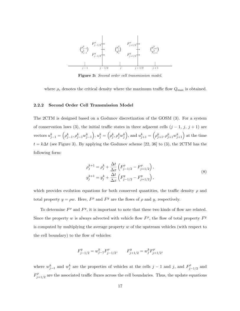
Figure 3: Second order cell transmission model.
where ρc denotes the critical density where the maximum traffic flow Qmax is obtained.
2.2.2 Second Order Cell Transmission Model
The 2CTM is designed based on a Godunov discretization of the GOSM (3). For a system
of conservation laws (3), the initial traffic states in three adjacent cells (j − 1, j, j + 1) are
vectors ukj−1 =(ρkj−1, ρ
kj−1w
kj−1
), ukj =
(ρkj , ρ
kjw
kj
), and ukj+1 =
(ρkj+1, ρ
kj+1w
kj+1
)at the time
t = k∆t (see Figure 3). By applying the Godunov scheme [22, 36] to (3), the 2CTM has the
following form:
ρk+1j = ρkj +
∆t
∆x
(F ρj−1/2 − F
ρj+1/2
),
yk+1j = ykj +
∆t
∆x
(F yj−1/2 − F
yj+1/2
),
(8)
which provides evolution equations for both conserved quantities, the traffic density ρ and
total property y = ρw. Here, F ρ and F y are the flows of ρ and y, respectively.
To determine F ρ and F y, it is important to note that these two kinds of flow are related.
Since the property w is always advected with vehicle flow F ρ, the flow of total property F y
is computed by multiplying the average property w of the upstream vehicles (with respect to
the cell boundary) to the flow of vehicles:
F yj−1/2 = wkj−1Fρj−1/2, F yj+1/2 = wkjF
ρj+1/2,
where wkj−1 and wkj are the properties of vehicles at the cells j − 1 and j, and F ρj−1/2 and
F ρj+1/2 are the associated traffic fluxes across the cell boundaries. Thus, the update equations
17
Sending function
traffic density
trafficflux
0 ρmaxρc(wL)0
q = Q(ρ, wL)
q = Q(ρ, wR)
sending function
(a)
Receiving function
traffic density
trafficflux
0 ρmaxρc(wL)0
q = Q(ρ, wL)
q = Q(ρ, wR)
receiving function
(b)
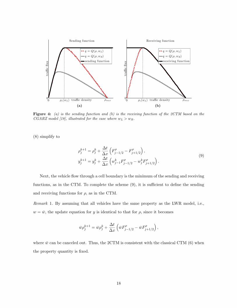
Figure 4: (a) is the sending function and (b) is the receiving function of the 2CTM based on theCGARZ model [18], illustrated for the case where wL > wR.
(8) simplify to
ρk+1j = ρkj +
∆t
∆x
(F ρj−1/2 − F
ρj+1/2
),
yk+1j = ykj +
∆t
∆x
(wkj−1F
ρj−1/2 − w
kjF
ρj+1/2
).
(9)
Next, the vehicle flow through a cell boundary is the minimum of the sending and receiving
functions, as in the CTM. To complete the scheme (9), it is sufficient to define the sending
and receiving functions for ρ, as in the CTM.
Remark 1. By assuming that all vehicles have the same property as the LWR model, i.e.,
w = w, the update equation for y is identical to that for ρ, since it becomes
wρk+1j = wρkj +
∆t
∆x
(wF ρj−1/2 − wF
ρj+1/2
),
where w can be canceled out. Thus, the 2CTM is consistent with the classical CTM (6) when
the property quantity is fixed.
18
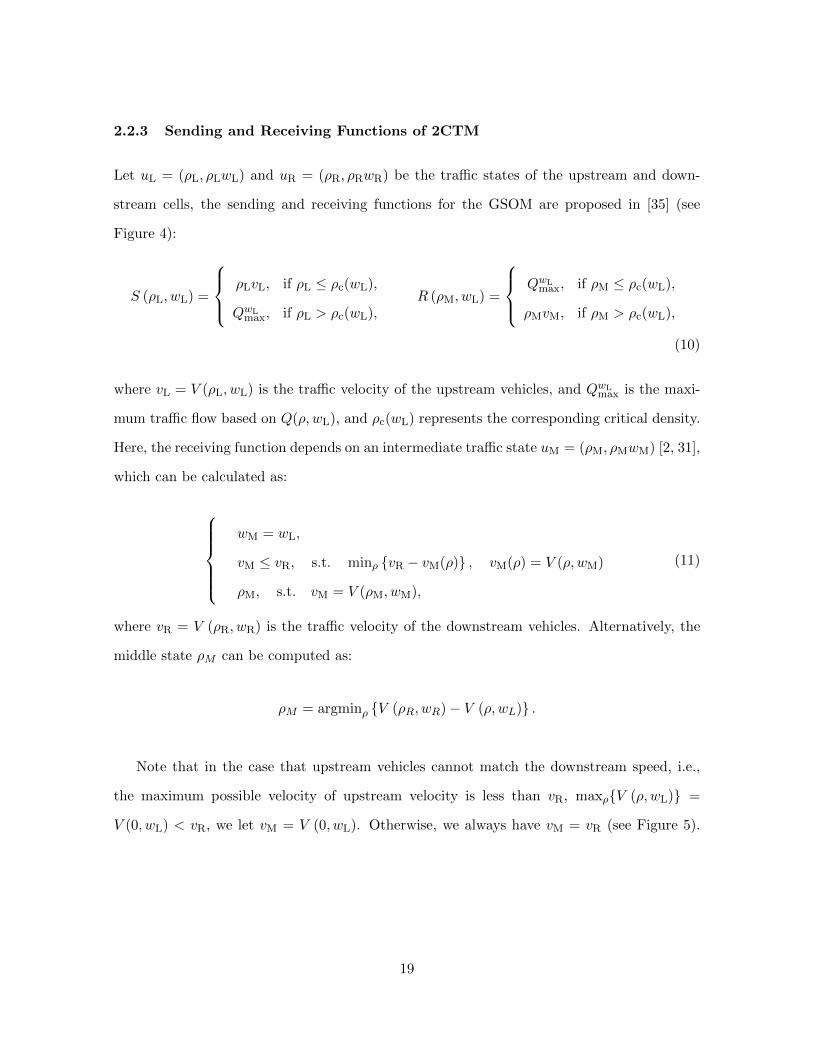
2.2.3 Sending and Receiving Functions of 2CTM
Let uL = (ρL, ρLwL) and uR = (ρR, ρRwR) be the traffic states of the upstream and down-
stream cells, the sending and receiving functions for the GSOM are proposed in [35] (see
Figure 4):
S (ρL, wL) =
ρLvL, if ρL ≤ ρc(wL),
QwLmax, if ρL > ρc(wL),
R (ρM, wL) =
QwLmax, if ρM ≤ ρc(wL),
ρMvM, if ρM > ρc(wL),
(10)
where vL = V (ρL, wL) is the traffic velocity of the upstream vehicles, and QwLmax is the maxi-
mum traffic flow based on Q(ρ, wL), and ρc(wL) represents the corresponding critical density.
Here, the receiving function depends on an intermediate traffic state uM = (ρM, ρMwM) [2, 31],
which can be calculated as:
wM = wL,
vM ≤ vR, s.t. minρ vR − vM(ρ) , vM(ρ) = V (ρ, wM)
ρM, s.t. vM = V (ρM, wM),
(11)
where vR = V (ρR, wR) is the traffic velocity of the downstream vehicles. Alternatively, the
middle state ρM can be computed as:
ρM = argminρ V (ρR, wR)− V (ρ, wL) .
Note that in the case that upstream vehicles cannot match the downstream speed, i.e.,
the maximum possible velocity of upstream velocity is less than vR, maxρV (ρ, wL) =
V (0, wL) < vR, we let vM = V (0, wL). Otherwise, we always have vM = vR (see Figure 5).
19
Thus, the solver (11) is rewritten as:
wM = wL,
vM = V (0, wL), if V (0, wL) < vR,
vM = vR, otherwise,
ρM, s.t. vM = V (ρM, wM).
(12)
The intuition behind this solver for the intermediate state is explained in more detail in the
next section.
From (10) and (12), the inflow of the jth cell is computed as:
F ρj−1/2 = minS(ρkj−1, w
kj−1
), R(ρkj−1/2, w
kj−1
), (13)
where ρkj−1/2 represents the intermediate density calculated from (12) given initial states ukj−1
and ukj . The outflow of the jth cell can be defined in the same way. The 2CTM is summarized
in Algorithm 1.
By comparing with the sending and receiving functions of the CTM (7), one notes that (i)
the sending function (10) depends only on the upstream traffic state uL, which is consistent
with the CTM; (ii) the receiving function depends on the intermediate density ρM (which
itself depends on the downstream speed vR and upstream property wL), and the upstream
property wL. It remains to provide a justification of the existence of the intermediate state
and an explanation of the dependence on the upstream property. These points are explored
in the next section.
2.2.4 Intermediate Traffic State
The existence of an intermediate state uM in the GSOM (3) can be understood as a conse-
quence of the interactions of vehicles with different properties w. Here, two adjacent cells (an
upstream cell and a downstream cell) with initial states uL and uR are studied. The traffic
flow through the cell interface is determined by the following rules:
20
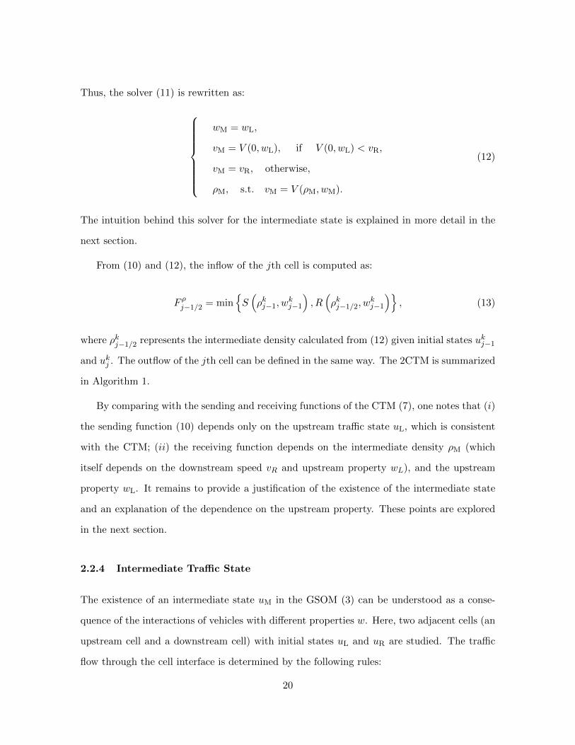
Algorithm 1 Second Order Cell Transmission Model
Current Time Step (t = k∆t): initial traffic states in cells j − 1, j, and j + 1: ukj−1 =(ρkj−1, ρ
kj−1w
kj−1
), ukj =
(ρkj , ρ
kjw
kj
), and ukj+1 =
(ρkj+1, ρ
kj+1w
kj+1
).
Intermediate State: Calculate the intermediate densities ρkj−1/2 (between ukj−1 and ukj )
and ρkj+1/2 (between ukj and ukj+1) from (12):
ρkj−1/2 = argminρ
V(ρkj , w
kj
)− V
(ρ, wkj−1
),
ρkj+1/2 = argminρ
V(ρkj+1, w
kj+1
)− V
(ρ, wkj
).
Inflow and Outflow: the inflow and outflow of the jth cell are computed using (10) and(13):
F ρj−1/2 = minS(ρkj−1, w
kj−1
), R(ρkj−1/2, w
kj−1
),
F ρj+1/2 = minS(ρkj , w
kj
), R(ρkj+1/2, w
kj
).
Next Time Step (t = (k + 1)∆t): the traffic density and the total property y = ρw areupdated to the next time step:
ρk+1j = ρkj +
∆t
∆x
(F ρj−1/2 − F
ρj+1/2
), yk+1
j = ykj +∆t
∆x
(wkj−1F
ρj−1/2 − w
kjF
ρj+1/2
).
Finally, the property is obtained as wk+1j = yk+1
j /ρk+1j .
1. Downstream vehicles move out of way, which creates spaces for the upstream vehicles.
Vehicles never move backwards.
2. Upstream vehicles maintain their property when moving from one cell to another. As
a result, wM = wL.
3. Vehicles from the upstream cell drive as fast as possible, but not faster than the down-
stream vehicles. This means that vM = vR whenever possible. Otherwise, vM is chosen
such that the gap between the velocities is minimized, i.e., minρ vR − vM(ρ), where
vM(ρ) = V (ρ, wM). Note vR depends on the downstream density and downstream prop-
erty, i.e., vR = V (ρR, wR).
4. Vehicles that flow through the cell interface with the property wL adjust their spacing
(density) to arrive the velocity vM determined from rule (3), which creates an interme-
21
Intermediate State
traffic density
trafficflux
0 ρmax0
q = Q(ρ, wL)
q = vRρ
Intermediate state
(a)
Intermediate State
traffic density
trafficflux
0 ρmax0
q = Q(ρ, wL)
q = vRρ
Intermediate state
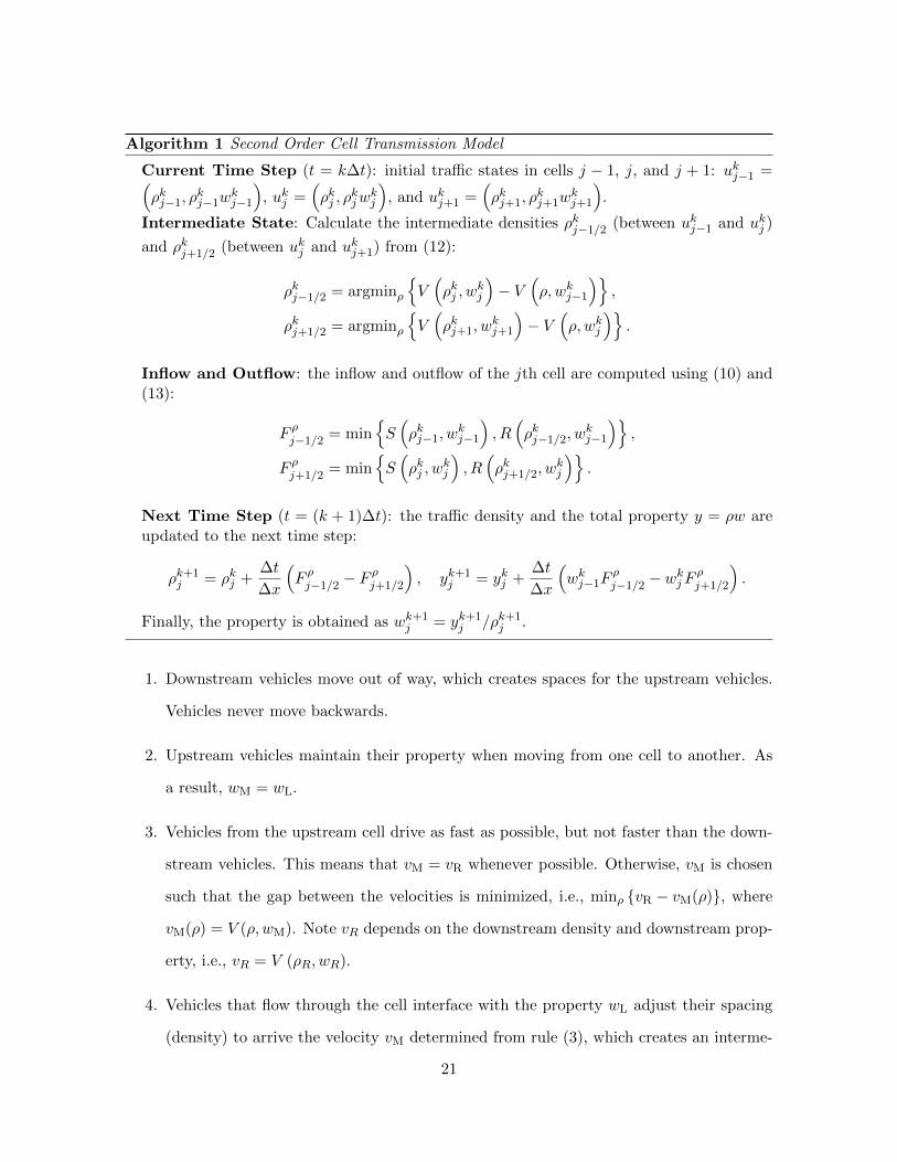
(b)
Figure 5: (a): upstream vehicles have the potential to match the downstream velocity, i.e., vR ≤V (0, wL) or vR ≤ Q′(0, wL), in which case vM = vR and (b): the maximum possible velocity ofupstream vehicles is lower than the downstream velocity, i.e., vR > V (0, wL) or vR > Q′(0, wL). Inthis case, let vM = V (0, wL) in order to minimize the gap to the downstream velocity.
diate density ρM, s.t., vM = V (ρM, wL).
These principles can be translated into the solver introduced in (11) and (12). One sees that
the solver for the intermediate state in the 2CTM is consistent with that of the Riemann
solver of the GOSM.
From the intuition to construct an intermediate traffic state, it is clear that the receiving
potential of the downstream cell is determined by both the space that the downstream ve-
hicles have created and the property of the upstream drivers. Considering an example that
the upstream drivers are quite passive, and in contrast, the downstream cell is filled with
aggressive drivers, then the receiving of vehicles depends not only on the amount of the space
that the downstream vehicles can generate (determined by uR), but also on the willingness
of the vehicles from the upstream cell to fill the free space (determined by wL). Therefore,
it is not surprising that the receiving function (10) is also a function of the property of the
upstream vehicles, which is different from the classical CTM.
22
2.2.5 A Multiple Model Framework for 2CTM
Next, a multiple model framework is proposed for the 2CTM by introducing the regime
variable µ to describe the number of open lanes. Thus, the flow through a cell interface is a
function of the regime variables of both the upstream and downstream cells. Following the
same updating equations as the 2CTM (9), the inflow and outflow are defined as:
F ρj−1/2 = minS(ρkj−1, w
kj−1, µ
k+1j−1
), R
(ρkj−1/2, w
kj−1, µ
k+1j
),
F ρj+1/2 = minS(ρkj , w
kj , µ
k+1j
), R
(ρkj+1/2, w
kj , µ
k+1j+1
),
where µk+1j−1 and µk+1
j are the regime variables of the cells j − 1 and j at time t = (k + 1)∆t,
and the sending and receiving functions (10) are modified to include the regime variable. Here
ρkj−1/2 and ρkj+1/2 are the intermediate states (see Section 2.2.4). Generally, for two adjacent
cells with traffic states uL and uR, the sending and receiving functions are:
S (ρL, wL, µL) =
ρLvL, if ρL ≤ µLρc(wL),
QwLmax(µL), if ρL > µLρc(wL),
R(ρM, wL, µR) =
QwLmax(µR), if ρM ≤ µRρc(wL),
ρM(µR)vM(µR), if ρM > µRρc(wL),
(14)
where vL = V (ρL, wL, µL) is the upstream traffic velocity, ρM(·) and vM(·) are the density
and velocity of the intermediate state, and QwLmax(µL) and QwL
max(µR) are the maximum fluxes
corresponding to the following flux function:
Q(ρ, w, µ) = ρV (ρ, w, µ) .
For example, one can define a velocity function as:
v = V (ρ, w, µ) =
vmax
(1− ρ
µρmax
), if ρ ≤ µρc(w),
Qwmax
µ(ρc(w)−ρmax(w))ρ−µρmax(w)
ρ , if ρ > µρc(w),(15)
23
where ρmax(w) = ρmax1ρmax2
wρmax1+(1−w)ρmax2and ρc(w) = ρc1ρc2
wρc1+(1−w)ρc2. Here, the model parameters
ρmax1, ρmax2, ρc1 and ρc2 are the upper and lower bounds of the jam density ρmax and the
critical density ρc, respectively, and ρmax defines the curvature of the FD in the freeflow
regime. All these parameters are defined with respect to a single lane, i.e., µ = 1, and
Qwmax = µρc(w)vmax
(1− ρc(w)
ρmax
).
Moreover, µLρc(wL) and µRρc(wL) are the corresponding critical densities such that these
maximum fluxes are obtained. Note that ρc(wL) is the critical density with respect to the
flux function of a single lane, i.e., µ = 1. The maximum flows are calculated as:
QwLmax(µL) = µLρc(wL)V (µLρc, wL, µL) , QwL
max (µR) = µRρc(wL)V (µRρc, wL, µR) .
Next, the intermediate traffic density and velocity ρM and vM are computed via a modified
version of (12):
wM = wL,
vM = V (0, wL, µR), if V (0, wL, µR) < vR,
vM = vR, otherwise,
ρM, s.t. vM = V (ρM, wM, µR),
(16)
where vR = V (ρR, wR, µR) is the velocity of the downstream vehicles.
Remark 2. In the definition of sending and receiving functions (14), the property is always
chosen as the upstream property wL. The sending function chooses the upstream regime
variable µL, and the receiving function selects the downstream regime variable µR.
2.3 A Multiple Model 2CTM on Road Network
In Section 2.2, a multiple model framework for the 2CTM based on the GOSM is presented
for a single road segment. It is desirable to generalize the model predictor to a road network
since all traffic problems are solved with respect a network that is composed of links and
junctions. In this case, a generalized Riemann problem is defined at each road junction. The
methodology to construct a unique admissible solution to the junction Riemann problem by
24
applying the GOSM or 2CTM is introduced next.
The key to compute the network solution requires defining a solution to a generalized
Riemann problem at a junction located at x0. Let the spatial domain of each incoming link i
be given as xi ∈(−∞, x−0,i
)and each outgoing link as xi ∈
(x+
0,i,+∞)
. Here, the point x−0,i
is the point on incoming link i which is immediately to the left of the junction at x0,i, and
x+0,i is the point on outgoing link i immediately to the right of the junction. The junction
Riemann problem is given as:
ρi
ρiwi
t
+
ρivi
ρiwivi
x
= 0, ui(x, 0) =
u−i if x < x−0,i,
u+i if x > x+
0,i,(17)
where ρi, wi and vi denote the density, property and velocity of vehicles on the ith link,
respectively, and ui(x, t) = (ρi(x, t), µi(x, t), ρi(x, t)wi(x, t)) is the traffic state, which is a
function of both position x and time t. Note that the regime variables µi are involved.
Moreover, u−i = (ρ−i , µ−i , ρ
−i w−i ) and u+
i = (ρ+i , µ
+i , ρ
+i w
+i ) represent the constant initial data
of the Riemann problem, and µ−i and µ+i are the regime variables on an incoming link and
an outgoing link.
The Rankine–Hugoniot conditions [24] are satisfied for piecewise constant solutions:
∑i∈δ−
(ρivi)(x−0,i, t
)=∑i∈δ+
(ρivi)(x+
0,i, t),
∑i∈δ−
(ρiviwi)(x−0,i, t
)=∑i∈δ+
(ρiviwi)(x+
0,i, t),
(18)
where δ− and δ+ are the sets of incoming links and outgoing links, respectively. These two
equations correspond to the conservation of mass ρ and conservation of the total property
y = ρw, respectively.
As pointed out in [20], condition (18) only is not sufficient to obtain a unique solution
for the Riemann problem of a junction when applying a second order traffic model. Hence,
additional conditions are necessary, such as: (i) a distribution parameter is specified that
25
determines the priority rules of vehicles at a road junction, i.e.,
0 ≤ ai,j ≤ 1,∑j∈δ+
ai,j = 1, ∀i ∈ δ−, (19)
where ai,j is the percentage of vehicles from the ith incoming link that goes to the jth outgoing
link; (ii) the total flux is maximized; (iii) the travel time is minimized. There are several other
restrictions that are motivated by mathematical convenience in order to generate a unique
solution at a junction. In this study, the distribution rule and traffic flow maximization rules
are used.
In the framework of the GOSM, the quantity w represents a property of vehicles, and thus
an admissible solution to a junction problem should guarantee that the upstream vehicles
(vehicles from incoming links) preserve their property passing through a junction [24]. For
example, drivers keep their property when driving from link i to link j. Recall the Remark 1
that the GOSM collapses to the LWR model by assuming a constant property. Similarly, it is
shown later that forcing vehicles to retain their property when traveling through the junction
is essential when solving a junction problem using the GOSM. When this is true, the junction
problems are structurally similar to junction problems for the first order LWR model [10, 11]
(excluding the merge problem).
Next, three types of junctions that are most common on a road network are studied:
bottlenecks (e.g., lane drop), diverges (e.g., off–ramp), and merges (e.g., on–ramp).
2.3.1 Bottleneck: One Incoming Link and One Outgoing Link
A bottleneck is a simple network that involves two links i = 1 (incoming) and i = 2 (outgoing).
Figure 6 shows a sample bottleneck junction where number of lanes changes from four lanes
to three. The constant initial data for (17) is
u−1 = (ρ−1 , µ−1 , ρ
−1 w−1 ), u+
2 = (ρ+2 , µ
+2 , ρ
+2 w
+2 ),
26
Bottleneck
f1f2
Figure 6: Bottleneck junction.
where u1(·) and u2(·) are traffic states on link 1 and link 2.
Vehicles with different properties interact with each other, and an intermediate state uM
is generated at the downstream side of the junction, i.e., at x+0,2 (see Section 2.2.4 for details).
One sees that the intermediate state has the same property as the upstream vehicles since
vehicles preserve their property, i.e., uM = (ρM, ρMw−1 ). Next, the junction problem is solved
between the states u−1 and uM, which have the same property w−1 . This is equivalent to a
junction problem for the LWR model.
The methodology to obtain a unique admissible solution to the junction problem applying
the LWR model is introduced in [10, 11]. In summary, one solves a maximization problem
max f
s.t. 0 ≤ f ≤ S1
(ρ−1 , w
−1 , µ
−1
),
0 ≤ f ≤ R2
(ρM, w
−1 , µ
+2
),
where f represents the realized flow across the junction, S1(·) is the sending function of link
1, and R2(·) represents the potential to receive vehicles on the link 2, which are defined in
(14). Here, the receiving function is a function of the intermediate density ρM obtained from
(16). Accordingly, the realized flow f∗ between the links is the minimum of the sending and
receiving functions:
f∗ = minS1
(ρ−1 , w
−1 , µ
−1
), R2
(ρM, w
−1 , µ
+2
).
27
Based on the solver to the junction problem introduced in [10, 11], one obtains u∗1 = (ρ∗1, ρ∗1w∗1)
and u∗2 = (ρ∗2, ρ∗2w∗2). Note that w∗1 = w∗2 = w−1 . Then, an inverse problem is solved to obtain
the densities given flows. The rules to obtain a unique solution are introduced in [10, 11].
For strictly concave flux functions, each flow value may correspond to two distinct densi-
ties, for a fixed property w and regime variable µ. On road i, one solves for density ρ∗i given
flow f∗i as follows:
Q(ρ∗i , wi, µi) = f∗i , Q(ρ∗i , wi, µi) = ρ∗iVi(ρ∗i , wi, µi),
where wi and µi are the property quantity and the regime variable on road i, and Vi(·) is
the velocity function of the road i. For a given flow f∗i , two distinct density solutions may
generated. The unique density solution is selected from the following rules. For the ith
incoming link, the density solution belongs to domain Diin that is defined as
ρ∗i ∈ Diin =
ρ−i∪(Λ(ρ−i ), µ−i ρmax(w−i )
], if 0 ≤ ρ−i ≤ µ
−i ρc(w
−i ),[
µ−i ρc(w−i ), µ−i ρmax(w−i )
], if µ−i ρc(w
−i ) ≤ ρ−i ≤ µ
−i ρmax(w−i ),
(20)
where ρ−i , w−i and µ−i represent the density, property and regime variable of the ith incoming
road, respectively, and ρc(·) and ρmax(·) are the critical density and the maximum density
that depend on w. Here, they are defined with respect to a single lane, i.e., µ = 1. Moreover,
Λ(·) is defined such that Q (ρ, w, µ) = Q (Λ(ρ), w, µ), for ρ ∈ [0, µρmax(w)]. For example,
Λ(0) = µiρmax(wi) on road i. Similarly, the unique density solution on the jth outgoing road
ρ∗j belongs to the domain Djout that is defined as
ρ∗j ∈ Djout =
[0, µ+
j ρc(w+j )], if 0 ≤ ρ+
j ≤ µ+j ρc(w
+j ),
ρ+j
∪[0, Λ(ρ+
j )), if µ+
j ρc(w+j ) ≤ ρ+
j ≤ µ+j ρmax(w+
j ),(21)
where where ρ+j , w+
j and µ+j are the density, property and regime variable of the jth outgoing
28
Diverge
f3
f1
f2
α
1 − α
(a)
Merge
f1
f2
f3
α
1 − α
(b)
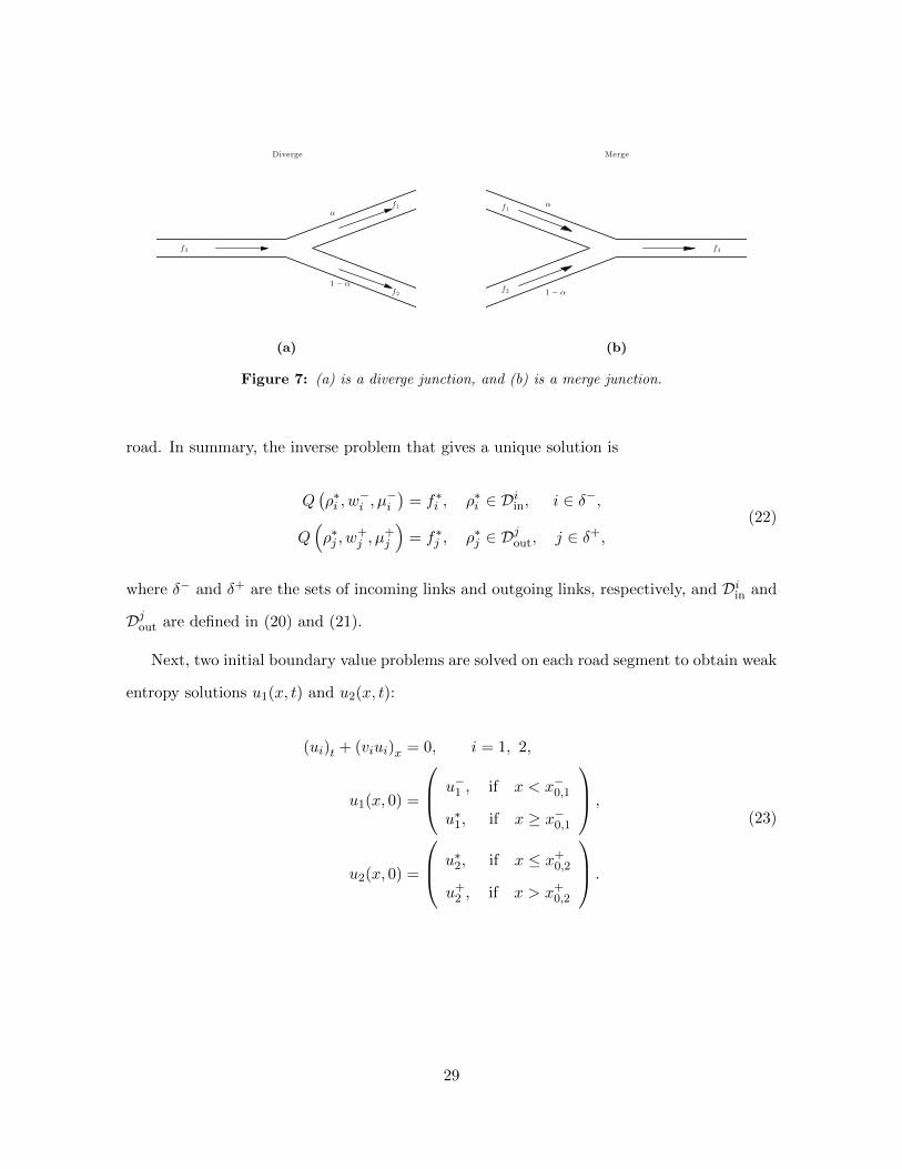
Figure 7: (a) is a diverge junction, and (b) is a merge junction.
road. In summary, the inverse problem that gives a unique solution is
Q(ρ∗i , w
−i , µ
−i
)= f∗i , ρ∗i ∈ Diin, i ∈ δ−,
Q(ρ∗j , w
+j , µ
+j
)= f∗j , ρ∗j ∈ D
jout, j ∈ δ+,
(22)
where δ− and δ+ are the sets of incoming links and outgoing links, respectively, and Diin and
Djout are defined in (20) and (21).
Next, two initial boundary value problems are solved on each road segment to obtain weak
entropy solutions u1(x, t) and u2(x, t):
(ui)t + (viui)x = 0, i = 1, 2,
u1(x, 0) =
u−1 , if x < x−0,1
u∗1, if x ≥ x−0,1
,
u2(x, 0) =
u∗2, if x ≤ x+0,2
u+2 , if x > x+
0,2
.
(23)
29
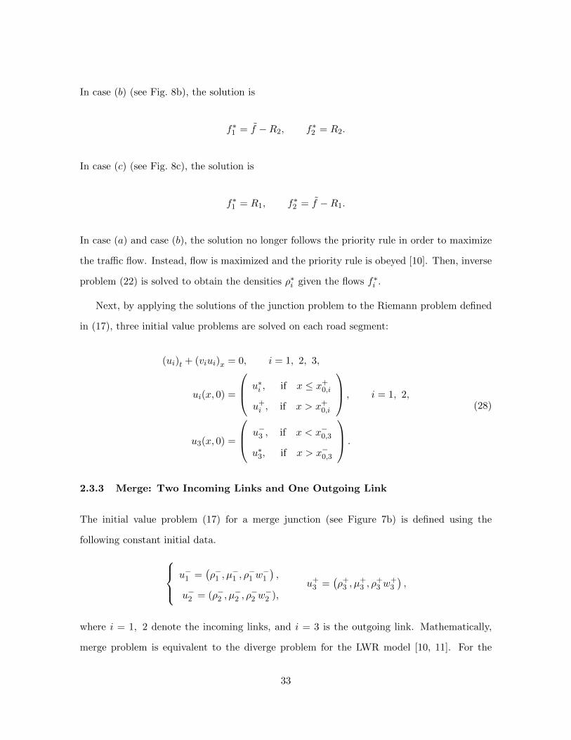
2.3.2 Diverge: One Incoming Link and Two Outgoing Links
The initial value problem (17) of a diverge junction (see Figure 7a) uses the following constant
initial data: u+1 = (ρ+
1 , µ+1 , ρ
+1 w
+1 ),
u+2 = (ρ+
2 , µ+2 , ρ
+2 w
+2 ),
u−3 = (ρ−3 , µ−3 , ρ
−3 w−3 ).
where i = 1, 2 represent the two outgoing links, and i = 3 denotes the incoming link. Similar
to the bottleneck problem, the Riemann problem of a diverge junction can also be reduced
to the classical network problem for the LWR model.
The solver proceeds in two steps:
1. Two intermediate states uMi =
(ρMi , ρ
Mi w
Mi
), i = 1, 2 are generated at the starting points
of two outgoing links, i.e., at the positions a1 and a2, with wM1 = wM
2 = w−3 . Again, these
intermediate states exist because drivers with different properties (from the upstream
or incoming links) try to match the velocity of the downstream vehicles (the outgoing
links) at a junction.
2. A junction problem is solved with initial data uM1 , uM
2 and u−3 . One sees that this is a
network problem based on the LWR model (see [10, 11] for detail) since the property
quantities are the same. The solutions are represented as u∗1, u∗2, and u∗3. In particular,
w∗1 = w∗2 = w∗3 = w−3 .
One refers to (16) to solve for the intermediate states in the first step. For the second step,
the allocation rule (19) is imposed to render a unique solution, as presented in [10, 11, 24].
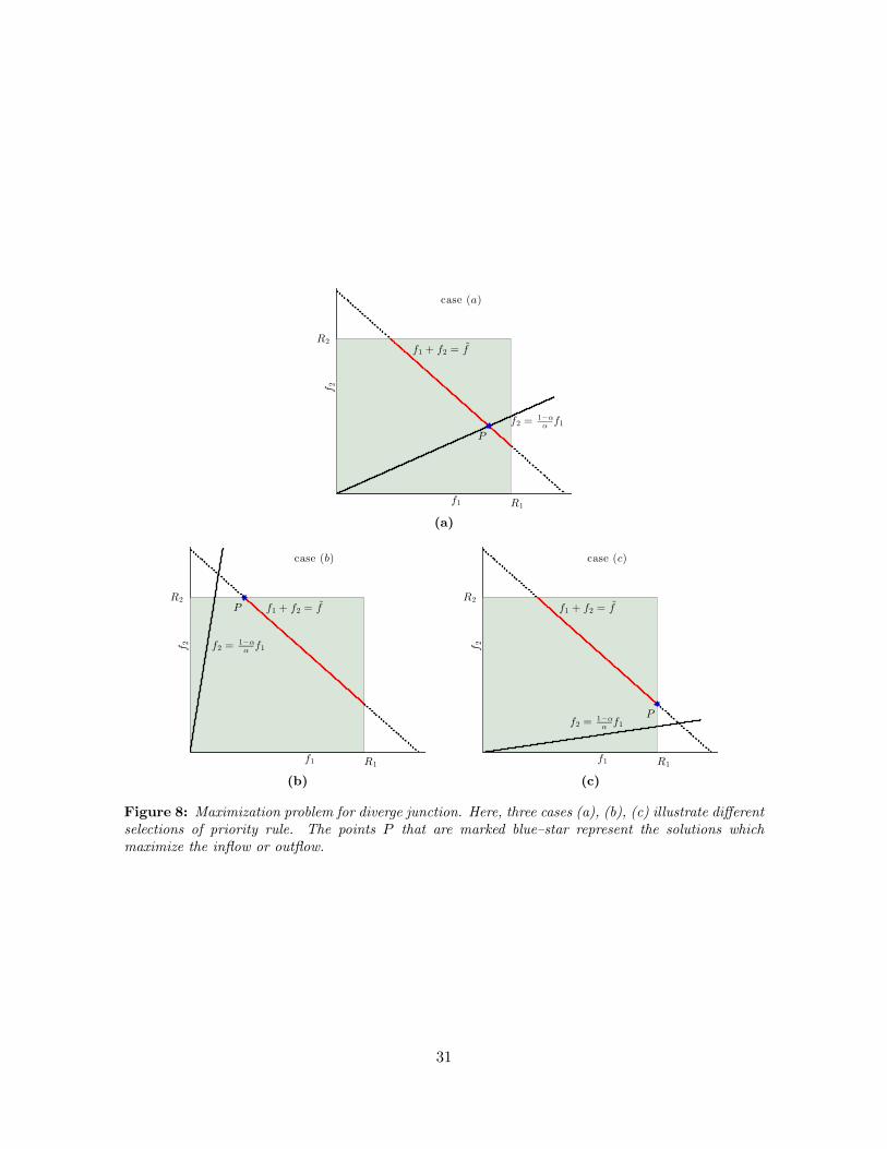
For a diverge problem, the following maximization problem is solved (see Figure 8):
max (f1 + f2)
s.t. 0 ≤fi ≤ Ri(ρMi , w
−3 , µ
+i
), i = 1, 2,
0 ≤f1 + f2 ≤ S3
(ρ−3 , w
−3 , µ
−3
),
(24)
where Ri(·), i = 1, 2 are the receiving functions on the outgoing links (downstream), and
30
P
case (a)
f1 + f2 = f
f2 =1−α
αf1
R1
R2
f1
f2
(a)
P
case (b)
f1 + f2 = f
f2 =1−α
αf1
R1
R2
f1
f2
(b)
P
case (c)
f1 + f2 = f
f2 =1−α
αf1
R1
R2
f1
f2
(c)
Figure 8: Maximization problem for diverge junction. Here, three cases (a), (b), (c) illustrate differentselections of priority rule. The points P that are marked blue–star represent the solutions whichmaximize the inflow or outflow.
31
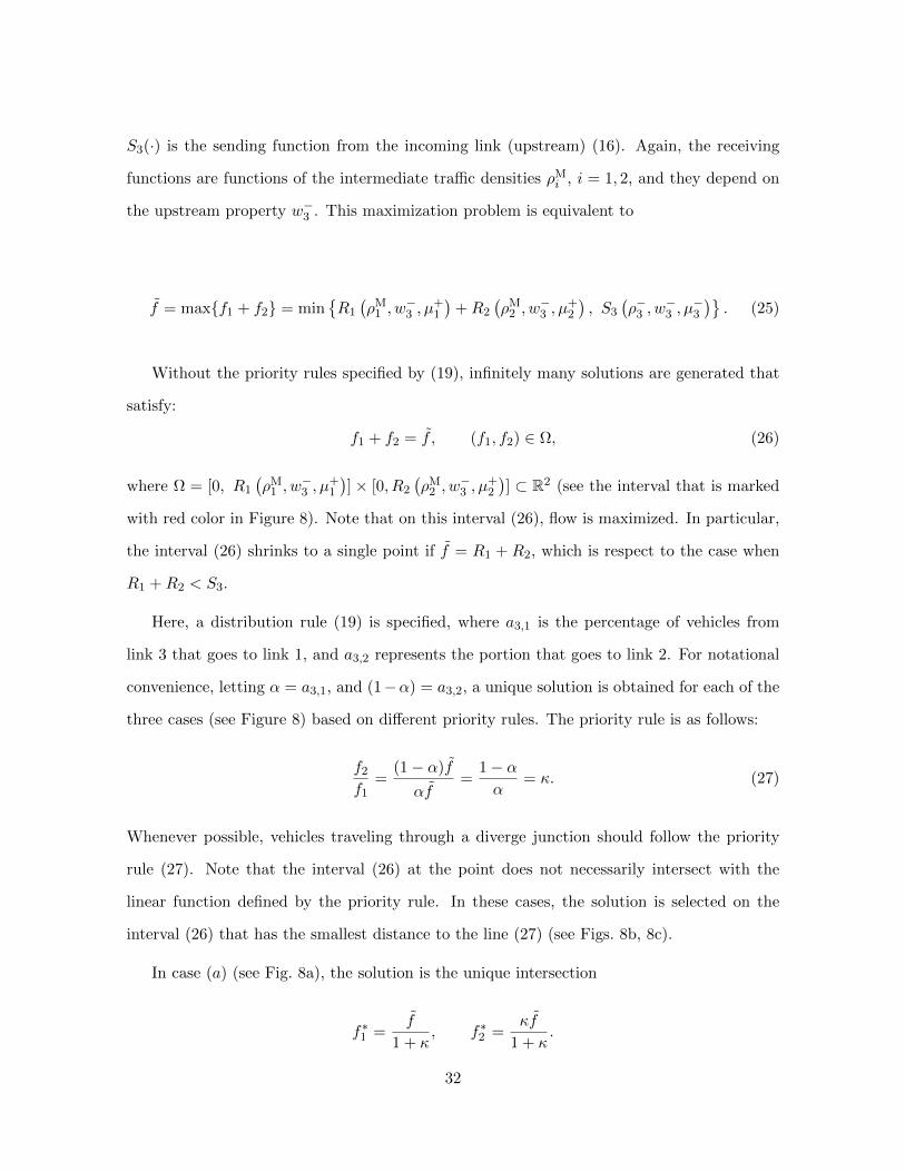
S3(·) is the sending function from the incoming link (upstream) (16). Again, the receiving
functions are functions of the intermediate traffic densities ρMi , i = 1, 2, and they depend on
the upstream property w−3 . This maximization problem is equivalent to
f = maxf1 + f2 = minR1
(ρM
1 , w−3 , µ
+1
)+R2
(ρM
2 , w−3 , µ
+2
), S3
(ρ−3 , w
−3 , µ
−3
). (25)
Without the priority rules specified by (19), infinitely many solutions are generated that
satisfy:
f1 + f2 = f , (f1, f2) ∈ Ω, (26)
where Ω = [0, R1
(ρM
1 , w−3 , µ
+1
)]× [0, R2
(ρM
2 , w−3 , µ
+2
)] ⊂ R2 (see the interval that is marked
with red color in Figure 8). Note that on this interval (26), flow is maximized. In particular,
the interval (26) shrinks to a single point if f = R1 + R2, which is respect to the case when
R1 +R2 < S3.
Here, a distribution rule (19) is specified, where a3,1 is the percentage of vehicles from
link 3 that goes to link 1, and a3,2 represents the portion that goes to link 2. For notational
convenience, letting α = a3,1, and (1−α) = a3,2, a unique solution is obtained for each of the
three cases (see Figure 8) based on different priority rules. The priority rule is as follows:
f2
f1=
(1− α)f
αf=
1− αα
= κ. (27)
Whenever possible, vehicles traveling through a diverge junction should follow the priority
rule (27). Note that the interval (26) at the point does not necessarily intersect with the
linear function defined by the priority rule. In these cases, the solution is selected on the
interval (26) that has the smallest distance to the line (27) (see Figs. 8b, 8c).
In case (a) (see Fig. 8a), the solution is the unique intersection
f∗1 =f
1 + κ, f∗2 =
κf
1 + κ.
32
In case (b) (see Fig. 8b), the solution is
f∗1 = f −R2, f∗2 = R2.
In case (c) (see Fig. 8c), the solution is
f∗1 = R1, f∗2 = f −R1.
In case (a) and case (b), the solution no longer follows the priority rule in order to maximize
the traffic flow. Instead, flow is maximized and the priority rule is obeyed [10]. Then, inverse
problem (22) is solved to obtain the densities ρ∗i given the flows f∗i .
Next, by applying the solutions of the junction problem to the Riemann problem defined
in (17), three initial value problems are solved on each road segment:
(ui)t + (viui)x = 0, i = 1, 2, 3,
ui(x, 0) =
u∗i , if x ≤ x+0,i
u+i , if x > x+
0,i
, i = 1, 2,
u3(x, 0) =
u−3 , if x < x−0,3
u∗3, if x > x−0,3
.
(28)
2.3.3 Merge: Two Incoming Links and One Outgoing Link
The initial value problem (17) for a merge junction (see Figure 7b) is defined using the
following constant initial data.
u−1 =(ρ−1 , µ
−1 , ρ
−1 w−1
),
u−2 = (ρ−2 , µ−2 , ρ
−2 w−2 ),
u+3 =
(ρ+
3 , µ+3 , ρ
+3 w
+3
),
where i = 1, 2 denote the incoming links, and i = 3 is the outgoing link. Mathematically,
merge problem is equivalent to the diverge problem for the LWR model [10, 11]. For the
33
GOSM, there is an important distinction between these two types of junctions: the property
on the outgoing link is defined in an average sense, which depends on the flows from the two
incoming links, i.e.,:
w∗3 =w−1 f1 + w−2 f2
f1 + f2, (29)
where w∗3 represents the property on the outgoing link, and f1 and f2 are the flows from two
incoming links.
To see this distinction more clearly, one investigates the following maximization problem:
max (f1 + f2)
s.t. 0 ≤fi ≤ Si(ρ−i , w
−i , µ
−i
), i = 1, 2,
0 ≤f1 + f2 ≤ R3
(ρM
3 , w∗3, µ
+3
), with ρM
3 = ρM3 (u+
3 , w∗3),
(30)
where the intermediate state ρM3 (·) is computed from (16), which depends on both the down-
stream state u+3 and the property of vehicles from the upstream wM
3 . Note that the maximiza-
tion problem (30) is a nonlinear optimization problem, since the receiving function depends
on w∗, which itself depends on f1 and f2. In this work, a different method is applied to obtain
a unique solution for the merge junction [24].
Based on the discussion in [24], the nonlinear optimization problem can be simplified to
a linear optimization problem by forcing the vehicles to follow the priority rule (19). Here,
the priority rule is recognized as a mixture rule that describes how vehicles of incoming links
mix when they enter the outgoing link. Let α be the percentage of vehicles from the first
incoming link, with α > 0, and (1 − α) be the portion of vehicles from the second incoming
link. The property on the outgoing link is given as
w∗3 = αw−1 + (1− α)w−2 , (31)
which is independent of the flows from two incoming links f1 and f2. Note that the mixture
rule in a merge problem must be satisfied, and therefore the flow is not necessarily maximized.
34
Fixing the priority rule, the following linear optimization problem is solved:
max (f1 + f2)
s.t. f2 = κf1,
0 ≤fi ≤ Si(ρ−i , w
−i , µ
−i
), i = 1, 2
0 ≤f1 + f2 ≤ R3
(ρM
3 , w∗3, µ
+3
),
(32)
where κ is defined as (27), and ρM3 is the intermediate state, where the property w∗3 is calcu-
lated by (31). The unique solution is therefore
f∗1 = min S1, S2/κ,R3/(1 + κ) , f∗2 = κf∗1 , f∗3 = (1 + κ)f∗1 . (33)
Next, the density solutions ρ∗i are obtained by solving the inverse problem (22). Moreover,
w∗1 = w−1 , w∗2 = w−2 , and w∗3 is determined by (31)
Similar to the diverge problem, the following initial value problems are solved:
(ui)t + (viui)x = 0, i = 1, 2, 3,
ui(x, 0) =
u−i , if x < x−0,i
u∗i , if x ≥ x−0,i
, i = 1, 2,
u3(x, 0) =
u∗3, if x ≤ x+0,3
u+3 , if x > x+
0,3
,
(34)
where u∗1, u∗2, and u∗3 are the solutions to the merge junction problem. Next, an approximate
solver to network problems is developed based on the multiple model 2CTM. As shown in the
next section, only the f∗ and w∗ are necessary in the discrete formulation.
Remark 3. The solution does not necessarily maximize the flow. For instance, consider the
case there are no vehicles on the first incoming link. The physically meaningful solution that
maximizes the traffic flow has f∗1 = 0. By (29), one obtains w∗3 = w−2 , which contradicts (31).
35
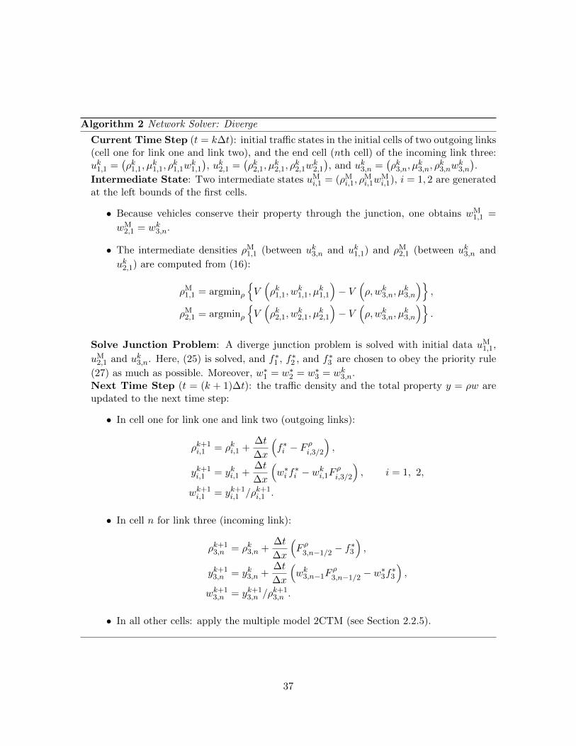
2.3.4 A Multiple Model Framework on a Road Network
In this section, the multiple model 2CTM on a road network is summarized.
Generally, one considers an incoming link i, where the cell adjacent to the junction is the
nth cell. The update equations for the nth cell on each link i is given by:
ρk+1i,n = ρki,n +
∆t
∆x
(F ρi,n−1/2 − f
∗i
),
yk+1i,n = yki,n +
∆t
∆x
(wki,n−1F
ρi,n−1/2 − w
∗i f∗i
).
(35)
where ρki,n and ρk+1i,n are traffic densities of the cell i, at time t = k∆t and t = (k + 1)∆t,
respectively, and yki,n and yk+1i,n are the associated quantities of total properties, e.g., yki,n =
wki,nρki,n, where wki,n represents the property of vehicles in the cell. Moreover, F ρi,n−1/2 is the
inflow of the cell i, and the outflow f∗i is the solution to the junction problem at the ith
incoming link. Furthermore, w∗i = wki,n, i.e., the property always follows that of the upstream
flow.
Similarly, for an outgoing link j, the evolution equations at the first cell of the jth outgoing
link are
ρk+1j,1 = ρkj,1 +
∆t
∆x
(f∗j − F
ρj,3/2
),
yk+1j,1 = ykj,1 +
∆t
∆x
(w∗jf
∗j − wkj,1F
ρj,3/2
),
(36)
where f∗j and F ρj,3/2 are the upstream and downstream flows of the cell. The inflow f∗j and
the upstream property w∗j are the solutions of the junction problem. The solvers for a diverge
network and a merge network are summarized in Algorithm 2 and Algorithm 3, respectively.
2.4 A Hybrid State Estimation Problem
The challenges for solving the proposed hybrid state estimation problem are due to the non-
linearities and switching dynamics associated with the traffic model. In the past, a number
of techniques in the estimation community have been developed to solve hybrid estimation
36
Algorithm 2 Network Solver: Diverge
Current Time Step (t = k∆t): initial traffic states in the initial cells of two outgoing links(cell one for link one and link two), and the end cell (nth cell) of the incoming link three:uk1,1 =
(ρk1,1, µ
k1,1, ρ
k1,1w
k1,1
), uk2,1 =
(ρk2,1, µ
k2,1, ρ
k2,1w
k2,1
), and uk3,n =
(ρk3,n, µ
k3,n, ρ
k3,nw
k3,n
).
Intermediate State: Two intermediate states uMi,1 = (ρM
i,1, ρMi,1w
Mi,1), i = 1, 2 are generated
at the left bounds of the first cells.
• Because vehicles conserve their property through the junction, one obtains wM1,1 =
wM2,1 = wk3,n.
• The intermediate densities ρM1,1 (between uk3,n and uk1,1) and ρM
2,1 (between uk3,n and
uk2,1) are computed from (16):
ρM1,1 = argminρ
V(ρk1,1, w
k1,1, µ
k1,1
)− V
(ρ, wk3,n, µ
k3,n
),
ρM2,1 = argminρ
V(ρk2,1, w
k2,1, µ
k2,1
)− V
(ρ, wk3,n, µ
k3,n
).
Solve Junction Problem: A diverge junction problem is solved with initial data uM1,1,
uM2,1 and uk3,n. Here, (25) is solved, and f∗1 , f∗2 , and f∗3 are chosen to obey the priority rule
(27) as much as possible. Moreover, w∗1 = w∗2 = w∗3 = wk3,n.Next Time Step (t = (k + 1)∆t): the traffic density and the total property y = ρw areupdated to the next time step:
• In cell one for link one and link two (outgoing links):
ρk+1i,1 = ρki,1 +
∆t
∆x
(f∗i − F
ρi,3/2
),
yk+1i,1 = yki,1 +
∆t
∆x
(w∗i f
∗i − wki,1F
ρi,3/2
), i = 1, 2,
wk+1i,1 = yk+1
i,1 /ρk+1i,1 .
• In cell n for link three (incoming link):
ρk+13,n = ρk3,n +
∆t
∆x
(F ρ3,n−1/2 − f
∗3
),
yk+13,n = yk3,n +
∆t
∆x
(wk3,n−1F
ρ3,n−1/2 − w
∗3f∗3
),
wk+13,n = yk+1
3,n /ρk+13,n .
• In all other cells: apply the multiple model 2CTM (see Section 2.2.5).
37
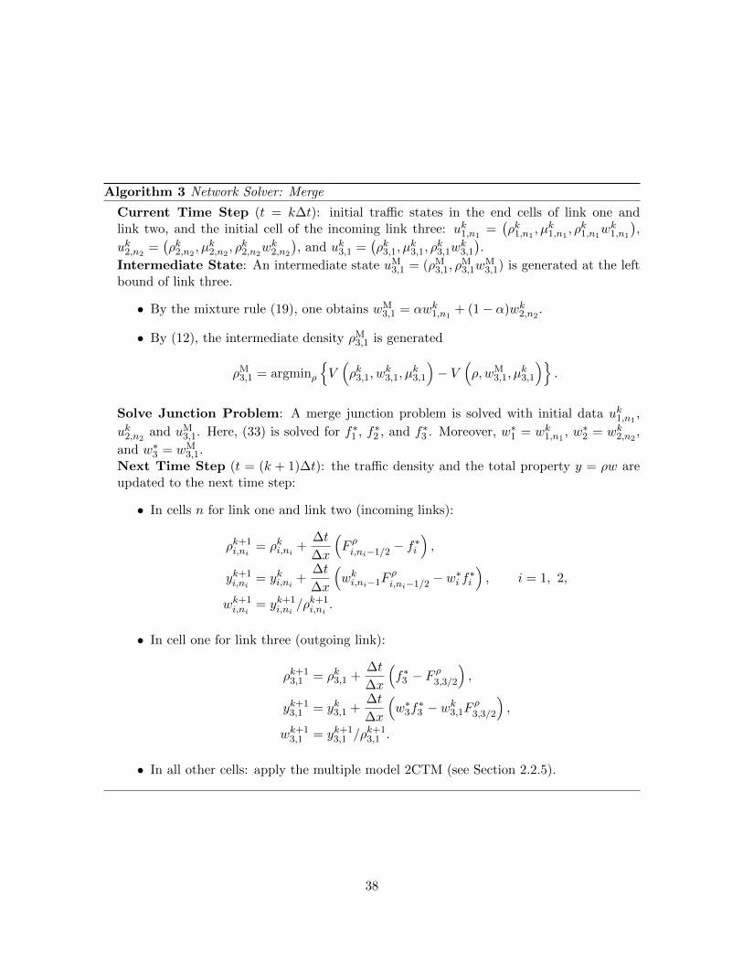
Algorithm 3 Network Solver: Merge
Current Time Step (t = k∆t): initial traffic states in the end cells of link one andlink two, and the initial cell of the incoming link three: uk1,n1
=(ρk1,n1
, µk1,n1, ρk1,n1
wk1,n1
),
uk2,n2=(ρk2,n2
, µk2,n2, ρk2,n2
wk2,n2
), and uk3,1 =
(ρk3,1, µ
k3,1, ρ
k3,1w
k3,1
).
Intermediate State: An intermediate state uM3,1 = (ρM
3,1, ρM3,1w
M3,1) is generated at the left
bound of link three.
• By the mixture rule (19), one obtains wM3,1 = αwk1,n1
+ (1− α)wk2,n2.
• By (12), the intermediate density ρM3,1 is generated
ρM3,1 = argminρ
V(ρk3,1, w
k3,1, µ
k3,1
)− V
(ρ, wM
3,1, µk3,1
).
Solve Junction Problem: A merge junction problem is solved with initial data uk1,n1,
uk2,n2and uM
3,1. Here, (33) is solved for f∗1 , f∗2 , and f∗3 . Moreover, w∗1 = wk1,n1, w∗2 = wk2,n2
,
and w∗3 = wM3,1.
Next Time Step (t = (k + 1)∆t): the traffic density and the total property y = ρw areupdated to the next time step:
• In cells n for link one and link two (incoming links):
ρk+1i,ni
= ρki,ni+
∆t
∆x
(F ρi,ni−1/2 − f
∗i
),
yk+1i,ni
= yki,ni+
∆t
∆x
(wki,ni−1F
ρi,ni−1/2 − w
∗i f∗i
), i = 1, 2,
wk+1i,ni
= yk+1i,ni
/ρk+1i,ni
.
• In cell one for link three (outgoing link):
ρk+13,1 = ρk3,1 +
∆t
∆x
(f∗3 − F
ρ3,3/2
),
yk+13,1 = yk3,1 +
∆t
∆x
(w∗3f
∗3 − wk3,1F
ρ3,3/2
),
wk+13,1 = yk+1
3,1 /ρk+13,1 .
• In all other cells: apply the multiple model 2CTM (see Section 2.2.5).
38
problems in the form of (1).
The multiple model particle filter (MMPF) [47] solves the hybrid state estimation problem
by allowing the system to have several models. It has a model transition step that describes
the switching dynamics of the system mode, and particles are generated for likely system
models. The idea of the MMPF is that if the state uk generated by a model variable µk
matches well with the measurements, then the estimator believes the system is operating
in model µ at time k. One central challenge for the MMPF to work in practice is due to
its large computational load. When a system has multiple models and some models have
very low probability of occurrence (e.g., system fault detection, traffic incident detection),
the estimation algorithm requires a large sample size so as to generate enough samples for
all possible models of the system. This will lead to a large computational load and possibly
prevent the algorithms from being implemented in real time. This problem is addressed by
[49], where a model–conditioned PF algorithm is proposed as an modification to the standard
MMPF. The computation time can be significantly reduced using this algorithm when a
hybrid state system contains rare modes.
Another group of the estimation techniques for solving the hybrid state estimation problem
exploits the multiple model (MM) approach and the Kalman filter. One of the widely used
approaches is the interactive multiple model (IMM) Kalman filter [7, 37, 43]. This method is a
model–conditioned Kalman filtering approach. It first computes the weights for all the models
of the hybrid system based on the switching probabilities among the models. Then, a Kalman
filter is performed on each model. The choice of the Kalman filter (e.g., extended Kalman
filter, EnKF, unscented Kalman filter) is problem dependent. The system state is estimated
by the estimation results from each model–conditioned Kalman filter and the weight of each
model computed by transitional probabilities among the system models.
Recently, the MMPF has been deployed for traffic state estimation and incident detection
in [51]. A multiple model particle filter is used to accommodate the nonlinearity and the
switching dynamics of the traffic incident model based on the scalar LWR traffic model. The
solution is a posterior distribution of system state u and system model µ. In this work, we
39
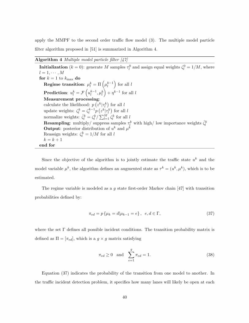
apply the MMPF to the second order traffic flow model (3). The multiple model particle
filter algorithm proposed in [51] is summarized in Algorithm 4.
Algorithm 4 Multiple model particle filter [47]
Initialization (k = 0): generate M samples τ0l and assign equal weights ζ0
l = 1/M , wherel = 1, · · · ,Mfor k = 1 to kmax do
Regime transition: µkl = Π(µk−1l
)for all l
Prediction: ukl = F(uk−1l , µkl
)+ ηk−1 for all l
Measurement processing:calculate the likelihood: p
(zk|τkl
)for all l
update weights: ζkl = ζk−1l p
(zk|τkl
)for all l
normalize weights: ζkl = ζkl /∑M
l=1 ζkl for all l
Resampling: multiply/ suppress samples τkl with high/ low importance weights ζklOutput: posterior distribution of uk and µk
Reassign weights: ζkl = 1/M for all lk = k + 1
end for
Since the objective of the algorithm is to jointly estimate the traffic state uk and the
model variable µk, the algorithm defines an augmented state as τk = (uk, µk), which is to be
estimated.
The regime variable is modeled as a g state first-order Markov chain [47] with transition
probabilities defined by:
πed = p µk = d|µk−1 = e , e, d ∈ Γ, (37)
where the set Γ defines all possible incident conditions. The transition probability matrix is
defined as Π = [πed], which is a g × g matrix satisfying
πed ≥ 0 and
g∑e=1
πed = 1. (38)
Equation (37) indicates the probability of the transition from one model to another. In
the traffic incident detection problem, it specifies how many lanes will likely be open at each
40
time step.
The MMPF works as follows. First, the algorithm constructs an initial distribution of the
augmented system state τk based on the prior knowledge. Here, the notation l is used to index
the particles. At the initial time step, all the particles are assigned with equal weights. Then,
according to the transition probability and the model variable from the previous time step,
for each particle, the algorithm determines the model variable for the current time step. Next,
the model prediction step is performed to calculate the prior distribution of the system state
uk. This gives the prediction by the traffic model. When the measurement for the current
time step is obtained, the algorithm computes the likelihood of each particle and updates the
weight of each particle based on the computed likelihood and its previous weight. Finally,
the algorithm resamples the particles based on their weights. During resampling, if a particle
has a high weight, the algorithm will generate more of that particle, while particles with low
weights are removed from the sample set.
The idea of the MMPF is that if a particle is generated by the correct model for the
current time step, it should match well with the measurements received from the sensor.
Consequently, the particle will be assigned with high weight and treated more importantly in
the posterior distribution. Similarly, if a particle is generated by a wrong model, it will not
match with well the measurements, and be assigned with less weight. Then, after resampling,
the particle will be removed from the sample set.
2.5 Simulation Results Based on CORSIM
We test the MMPF (Algorithm 4) applied to a second order traffic flow model (3) through
a numerical experiment using CORSIM, where the true state is known. CORSIM is a mi-
croscopic traffic simulation software developed by the Federal Highway Administration [42],
which is constructed from car–following and lane switching models. This microscopic sim-
ulator is very different from the second order macroscopic traffic flow model used in the
estimation algorithm, and therefore provides a more realistic simulation platform to test the
41
0 2 4 6 8Cell Number
0
50
100
150
Tim
e S
tep
050100150200250300350400450
(a) Density (veh/mile)
0 2 4 6 8Cell Number
0
50
100
150
Tim
e S
tep
0.0
0.3
0.6
0.9
1.2
1.5
1.8
2.1
2.4
2.7
3.0
(b) Model variable (lanes open)
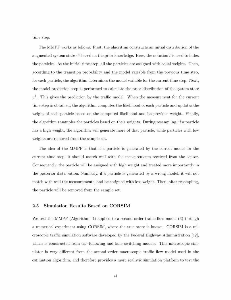
Figure 9: True evolution of the traffic density and the model variable.
algorithm.
To generate the true state to be estimated, a CORSIM simulation is performed on a 4
mile highway with a speed limit of 65 mph. The simulation time is one hour (180 30-second
timesteps). An incident is created in cell four, which is 1.36 miles from the starting point
of the highway. The incident starts 20 minutes after the simulation starts and lasts for 20
minutes (i.e. from time step 60 to time step 120 in the traffic model). The evolutions of the
traffic density and model parameter are shown in Figs. 9a and 9b.
Next, synthetic GPS measurements are created by extracting the trajectory data from
the CORSIM simulation. Various subsets of the vehicles are selected as probe vehicles, and
speed measurements are generated from these vehicles to simulate GPS measurements. In
this work, the penetration rate of GPS equipped vehicles is specified by adjusting the headway
between these vehicles.
In order to run the second order traffic flow model, the fundamental diagram shape and
parameters must be determined. Because the velocity function must be strictly decreasing
with respect to the density in the second order model, a piecewise quadratic fundamental
42
diagram is selected:
Q(ρ, w, µ) =
vmaxρ (1− ρ/µρ) if ρ ≤ µρc
a(w, µ)ρ2 + b(w, µ)ρ+ c(w, µ) if ρ ≥ µρc,(39)
To calibrate the parameters of the fundamental diagram, a number of CORSIM simu-
lations were generated under a range of different traffic conditions. In each simulation, the
densities and speeds were recorded to simulate data available from an inductive loop detec-
tor. To fit this data, the parameters of the fundamental diagram were set as vmax = 65
mph, ρmax ranges from 235-245 vpm/lane, Qmax ranges from 2100 - 2700 vph/lane, and ρ
is 30000 vpm/lane. The large value of ρ forces the quadratic function in free flow to closely
approximate a linear function. Finally, the parameters a, b, and c in (39) are a function of w
and can be determined by solving the following system of equations:
aµρmax(w)2 + bµρmax(w) + c = 0
− b2a = µQw
maxvmax
4ac−b24a = µQwmax,
(40)
where ρmax(w) = wρmax1 + (1 − w)ρmax2 and Qwmax = wqmax1 + (1 − w)qmax2 Here, ρmax1
and ρmax2 are the upper and lower bounds of the maximum traffic density, qmax1 and qmax2
are the upper of lower bounds of the maximum flow in the second order traffic model. The
resulting fundamental diagram for the second order traffic model is shown in Figure 10 for
several values of w.
Several numerical experiments are run by implementing the MMPF on the second order
traffic model, and generating measurements uisng different headways between GPS vehicles.
In the numerical simulation, we run the proposed algorithm with 1000 particles. We assume
there is no incident with 99 percent probability, and there is only only incident at a time. All
incident models are equally likely. With these assumptions, the transitional probability can
be constructed. In CORSIM, the left boundary condition is set as 7000veh/hour and the right
43
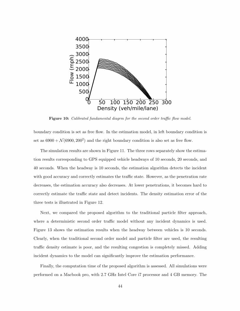
0 50 100 150 200 250 300Density (veh/mile/lane)
0500
1000150020002500300035004000
Flow
(m
ph)
Figure 10: Calibrated fundamental diagrm for the second order traffic flow model.
boundary condition is set as free flow. In the estimation model, in left boundary condition is
set as 6900 +N (6900, 2002) and the right boundary condition is also set as free flow.
The simulation results are shown in Figure 11. The three rows separately show the estima-
tion results corresponding to GPS equipped vehicle headways of 10 seconds, 20 seconds, and
40 seconds. When the headway is 10 seconds, the estimation algorithm detects the incident
with good accuracy and correctly estimates the traffic state. However, as the penetration rate
decreases, the estimation accuracy also decreases. At lower penetrations, it becomes hard to
correctly estimate the traffic state and detect incidents. The density estimation error of the
three tests is illustrated in Figure 12.
Next, we compared the proposed algorithm to the traditional particle filter approach,
where a deterministic second order traffic model without any incident dynamics is used.
Figure 13 shows the estimation results when the headway between vehicles is 10 seconds.
Clearly, when the traditional second order model and particle filter are used, the resulting
traffic density estimate is poor, and the resulting congestion is completely missed. Adding
incident dynamics to the model can significantly improve the estimation performance.
Finally, the computation time of the proposed algorithm is assessed. All simulations were
performed on a Macbook pro, with 2.7 GHz Intel Core i7 processor and 4 GB memory. The
44
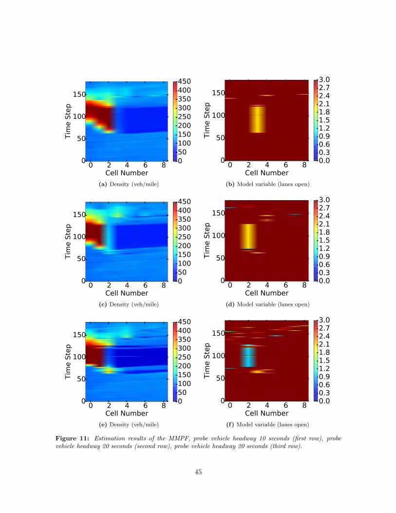
0 2 4 6 8Cell Number
0
50
100
150
Tim
e S
tep
050100150200250300350400450
(a) Density (veh/mile)
0 2 4 6 8Cell Number
0
50
100
150
Tim
e S
tep
0.00.30.60.91.21.51.82.12.42.73.0
(b) Model variable (lanes open)
0 2 4 6 8Cell Number
0
50
100
150
Tim
e S
tep
050100150200250300350400450
(c) Density (veh/mile)
0 2 4 6 8Cell Number
0
50
100
150Tim
e S
tep
0.00.30.60.91.21.51.82.12.42.73.0
(d) Model variable (lanes open)
0 2 4 6 8Cell Number
0
50
100
150
Tim
e S
tep
050100150200250300350400450
(e) Density (veh/mile)
0 2 4 6 8Cell Number
0
50
100
150
Tim
e S
tep
0.00.30.60.91.21.51.82.12.42.73.0
(f) Model variable (lanes open)
Figure 11: Estimation results of the MMPF, probe vehicle headway 10 seconds (first row), probevehicle headway 20 seconds (second row), probe vehicle headway 20 seconds (third row).
45
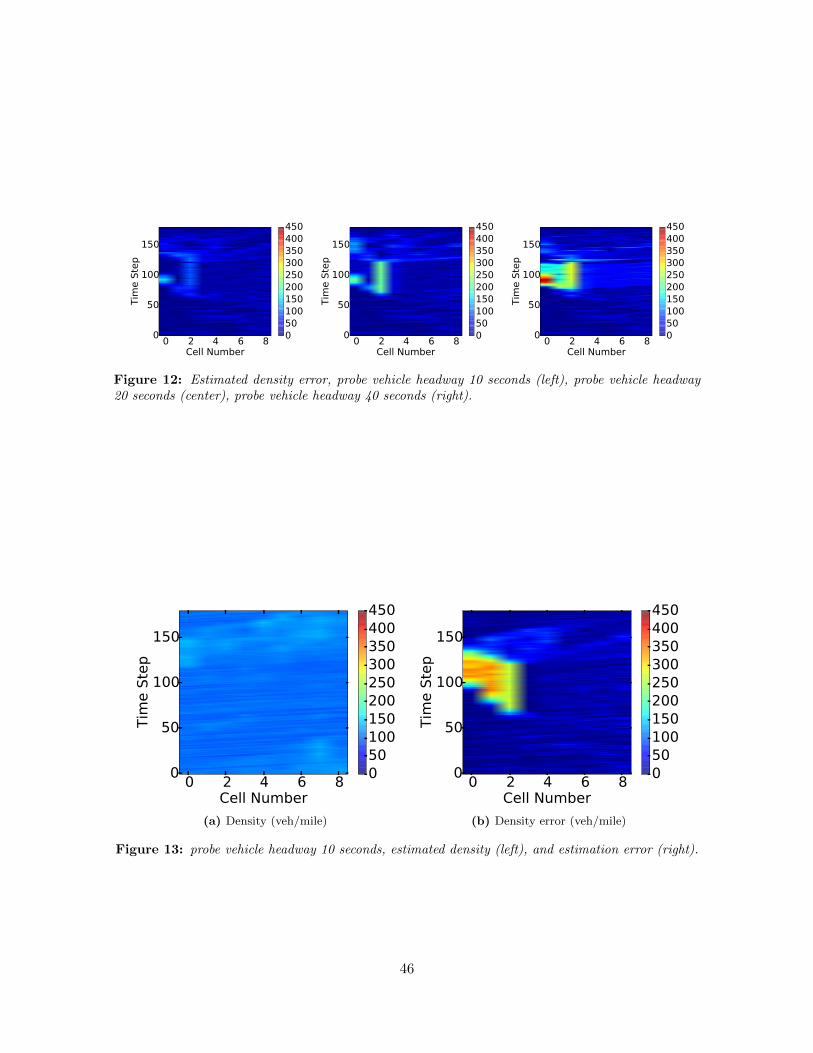
0 2 4 6 8Cell Number
0
50
100
150
Tim
e S
tep
050100150200250300350400450
0 2 4 6 8Cell Number
0
50
100
150
Tim
e S
tep
050100150200250300350400450
0 2 4 6 8Cell Number
0
50
100
150
Tim
e S
tep
050100150200250300350400450
Figure 12: Estimated density error, probe vehicle headway 10 seconds (left), probe vehicle headway20 seconds (center), probe vehicle headway 40 seconds (right).
0 2 4 6 8Cell Number
0
50
100
150
Tim
e S
tep
050100150200250300350400450
(a) Density (veh/mile)
0 2 4 6 8Cell Number
0
50
100
150
Tim
e S
tep
050100150200250300350400450
(b) Density error (veh/mile)
Figure 13: probe vehicle headway 10 seconds, estimated density (left), and estimation error (right).
46
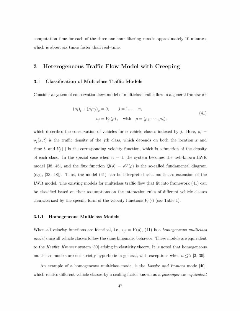
computation time for each of the three one-hour filtering runs is approximately 10 minutes,
which is about six times faster than real–time.
3 Heterogeneous Traffic Flow Model with Creeping
3.1 Classification of Multiclass Traffic Models
Consider a system of conservation laws model of multiclass traffic flow in a general framework
(ρj)t + (ρjvj)x = 0, j = 1, · · · , n,
vj = Vj (ρ) , with ρ = (ρ1, · · · , ρn) ,
(41)
which describes the conservation of vehicles for n vehicle classes indexed by j. Here, ρj =
ρj(x, t) is the traffic density of the jth class, which depends on both the location x and
time t, and Vj (·) is the corresponding velocity function, which is a function of the density
of each class. In the special case when n = 1, the system becomes the well-known LWR
model [38, 46], and the flux function Q(ρ) = ρV (ρ) is the so-called fundamental diagram
(e.g., [23, 48]). Thus, the model (41) can be interpreted as a multiclass extension of the
LWR model. The existing models for multiclass traffic flow that fit into framework (41) can
be classified based on their assumptions on the interaction rules of different vehicle classes
characterized by the specific form of the velocity functions Vj (·) (see Table 1).
3.1.1 Homogeneous Multiclass Models
When all velocity functions are identical, i.e., vj = V (ρ), (41) is a homogeneous multiclass
model since all vehicle classes follow the same kinematic behavior. These models are equivalent
to the Keyfitz–Kranzer system [30] arising in elasticity theory. It is noted that homogeneous
multiclass models are not strictly hyperbolic in general, with exceptions when n ≤ 2 [3, 30].
An example of a homogeneous multiclass model is the Logghe and Immers mode [40],
which relates different vehicle classes by a scaling factor known as a passenger car equivalent
47
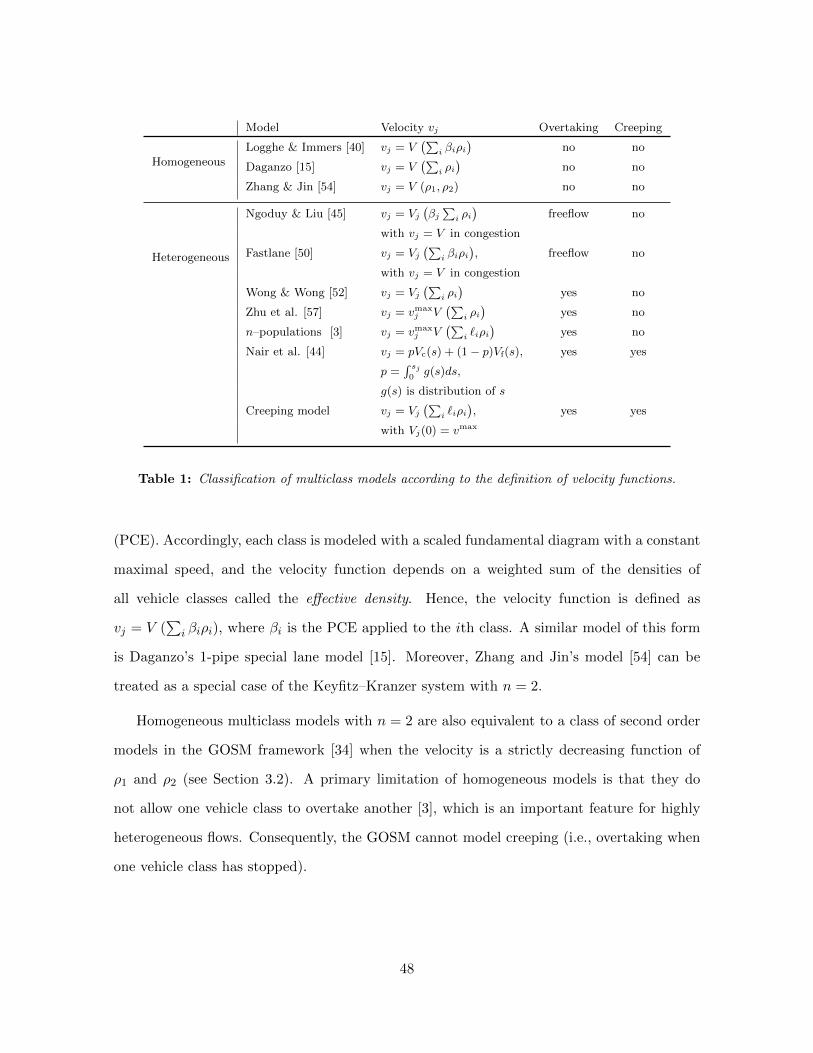
Model Velocity vj Overtaking Creeping
HomogeneousLogghe & Immers [40] vj = V
(∑i βiρi
)no no
Daganzo [15] vj = V(∑
i ρi)
no no
Zhang & Jin [54] vj = V (ρ1, ρ2) no no
Heterogeneous
Ngoduy & Liu [45] vj = Vj
(βj∑
i ρi)
freeflow no
with vj = V in congestion
Fastlane [50] vj = Vj
(∑i βiρi
), freeflow no
with vj = V in congestion
Wong & Wong [52] vj = Vj
(∑i ρi)
yes no
Zhu et al. [57] vj = vmaxj V
(∑i ρi)
yes no
n–populations [3] vj = vmaxj V
(∑i `iρi
)yes no
Nair et al. [44] vj = pVc(s) + (1 − p)Vf(s), yes yes
p =∫ sj0g(s)ds,
g(s) is distribution of s
Creeping model vj = Vj
(∑i `iρi
), yes yes
with Vj(0) = vmax
Table 1: Classification of multiclass models according to the definition of velocity functions.
(PCE). Accordingly, each class is modeled with a scaled fundamental diagram with a constant
maximal speed, and the velocity function depends on a weighted sum of the densities of
all vehicle classes called the effective density. Hence, the velocity function is defined as
vj = V (∑
i βiρi), where βi is the PCE applied to the ith class. A similar model of this form
is Daganzo’s 1-pipe special lane model [15]. Moreover, Zhang and Jin’s model [54] can be
treated as a special case of the Keyfitz–Kranzer system with n = 2.
Homogeneous multiclass models with n = 2 are also equivalent to a class of second order
models in the GOSM framework [34] when the velocity is a strictly decreasing function of
ρ1 and ρ2 (see Section 3.2). A primary limitation of homogeneous models is that they do
not allow one vehicle class to overtake another [3], which is an important feature for highly
heterogeneous flows. Consequently, the GOSM cannot model creeping (i.e., overtaking when
one vehicle class has stopped).
48
3.1.2 Heterogeneous Multiclass Models
Many research efforts are devoted to the design of heterogeneous multiclass models by dis-
tinguishing Vj(·) for each class. The model by Ngoduy and Liu [45] characterizes vehicle
classes by their maximum velocities, and assumes that the freeflow velocity depends on a
PCE–scaled density, i.e., vj = Vj (βj∑
i ρi), where βj is the PCE factor of the jth class. The
model uses the same velocity function for all classes in congestion. The Fastlane model [50]
also supposes that all vehicle classes have distinct velocity functions in freeflow but the same
function in congestion, however, it defines the velocity as a function of the effective density
(e.g., vj = Vj (∑
i βiρi)). As a consequence, the Ngoduy and Liu and Fastlane models [45, 50]
allow overtaking in the freeflow regime, but not in congestion.
Wong and Wong [52] introduced a simplified heterogeneous multiclass model of the form
(41) that admits overtaking in freeflow and congestion. The velocity function of each class is
a function of the total density (e.g. vj = Vj (∑
i ρi)) and they are distinct except at the jam
density. The model of Zhu et al. [57] also follows the same principle. Later, Benzoni–Gavage
and Colombo [3] introduced the n–populations model, which extended Wong and Wong’s
model [52] by explicitly taking the size of each vehicle class into account. Hence, the PCE
is chosen as the average length of each vehicle class `j . Instead of explicitly conserving the
number of vehicles, the system expresses conservation of the space occupied by each vehicle
class. Consequently, the velocity function depends on the total occupied space r =∑
j `jρj ,
i.e., vj = Vj (r). As presented in [3], by substituting ρj := `jρj in the n–populations model,
both models [3, 52] fit into the same mathematical framework
(ρj)t + (ρjvj)x = 0, j = 1, · · · , n,
vj = Vj(r), with r =
n∑j=1
ρj .(42)
The models [3, 52, 57] suppose all vehicle classes either never stop [52], or stop at a common
maximum occupied space rmax (or equivalently an effective jam density), i.e., Vj(rmax) = 0,
49
j = 1, · · · , n. In circumstances when the vehicles are highly heterogeneous in size, this as-
sumption may be violated. Indeed, one can observe that at a certain level of congestion, larger
vehicles such as cars and buses completely stop, while smaller vehicles such as motorcycles
continue to move through the gaps between the large vehicles. This creeping behavior can be
interpreted as a special lane which can only be used by small vehicles.
A heterogeneous multiclass model that allows for creeping is proposed by Nair et al. [44],
which also fits into the generic framework (42). In this model, the velocity of each vehicle
class is determined by the availability of empty spaces s (pores) for which vehicles of various
sizes compete. Letting sj represent a critical pore size for the jth class, vehicles may be in
freeflow (s ≥ sj) or congestion (s < sj) with velocity functions Vf(·) and Vc(·), respectively.
The overall velocity of the jth class is
vj = Vj (s) =
(∫ ∞sj
g(ω)dω
)Vf(s) +
(∫ sj
0g(ω)dω
)Vr(s), (43)
where g(·) is the probability density function of the pores sizes for a given time, and Vc(s) ≤
Vf(s). The creeping property is shown by numerical simulations for a flow with two vehicle
classes, but significant analytical results are missing due to the complexity of the model (43),
e.g., the density function g(s) evolves with time. Interestingly, the model [44] reduces to
homogeneous multiclass model when Vc(s) = Vf(s).
In this study, a two class heterogeneous model that exhibits creeping is proposed. To
understand the reason why second order traffic models (GOSM) are not suitable to model
creeping, a connection between the GOSM and the two class homogeneous multiclass traffic
model is established next.
3.2 Interpretation of the GOSM as a Two Class Homogeneous Multiclass
Model
As pointed out in [4, 17, 19], the GOSM [17, 34] (3) can be interpreted as a second order gen-
eralization of the LWR model, which allows for different vehicle properties such as aggressivity
50
[16]. In the GOSM framework, vehicles with the property w adjust their spacing s = 1/ρ for
a given velocity level v, where ρ is determined such that v = V (ρ, w). An aggressive driver
tends to select a smaller space when traveling at the same speed as a passive driver.
Similarly, the various interaction behaviors among different classes in multiclass flow can
also be interpreted as an assignment of road space to vehicle classes [41]. Hence, it is possible
to link two class heterogeneous models with the ARZ model. Consider a multiclass flow that
is composed of cars (j = 1) and trucks (j = 2). By letting ρ = (ρ1 + ρ2) be the total density
and defining w = ρ1/ρ as the fraction of vehicles in the first class, the second equation in (3)
is simply a conservation law for the first class, i.e., y = ρw = ρ1. Note that it is equivalent to
set the property as the fraction of the second vehicle class, i.e., w = ρ2/ρ. Thus, the GOSM
(3) becomes
(ρ)t +(ρV (ρ, ρ1/ρ)
)x
= 0,
(ρ1)t +(ρ1V (ρ1, ρ1/ρ)
)x
= 0.
(44)
By subtracting the second equation from the first one in (44), one obtains Zhang and Jin’s
[54] homogeneous two class model
(ρ1)t +(ρ1V (ρ1, ρ2)
)x
= 0,
(ρ2)t +(ρ2V (ρ1, ρ2)
)x
= 0,
(45)
with V (ρ1, ρ2) = V (ρ1 + ρ2, ρ1/(ρ1 + ρ2)). Furthermore, one verifies that the requirement
∂ρV < 0 in the GOSM is met under a sufficient condition:
∂ρ1 V (ρ1, ρ2) < 0, and ∂ρ2 V (ρ1, ρ2) < 0. (46)
Thus, the GOSM is equivalent to a two class homogeneous multiclass model of the form (45)
under the condition (46). Note that v = V (ρ, w), w = ρ1/ρ generates a family of velocity
curves that is parametrized by the fraction of cars. As the fraction of cars increases for a
fixed total density ρ, the velocity curve shifts upwards.
51
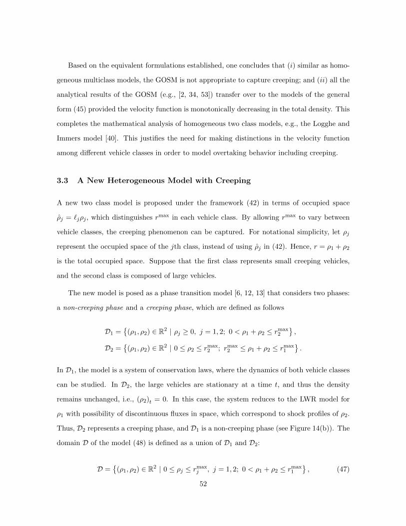
Based on the equivalent formulations established, one concludes that (i) similar as homo-
geneous multiclass models, the GOSM is not appropriate to capture creeping; and (ii) all the
analytical results of the GOSM (e.g., [2, 34, 53]) transfer over to the models of the general
form (45) provided the velocity function is monotonically decreasing in the total density. This
completes the mathematical analysis of homogeneous two class models, e.g., the Logghe and
Immers model [40]. This justifies the need for making distinctions in the velocity function
among different vehicle classes in order to model overtaking behavior including creeping.
3.3 A New Heterogeneous Model with Creeping
A new two class model is proposed under the framework (42) in terms of occupied space
ρj = `jρj , which distinguishes rmax in each vehicle class. By allowing rmax to vary between
vehicle classes, the creeping phenomenon can be captured. For notational simplicity, let ρj
represent the occupied space of the jth class, instead of using ρj in (42). Hence, r = ρ1 + ρ2
is the total occupied space. Suppose that the first class represents small creeping vehicles,
and the second class is composed of large vehicles.
The new model is posed as a phase transition model [6, 12, 13] that considers two phases:
a non-creeping phase and a creeping phase, which are defined as follows
D1 =
(ρ1, ρ2) ∈ R2 | ρj ≥ 0, j = 1, 2; 0 < ρ1 + ρ2 ≤ rmax2
,
D2 =
(ρ1, ρ2) ∈ R2 | 0 ≤ ρ2 ≤ rmax2 ; rmax
2 ≤ ρ1 + ρ2 ≤ rmax1
.
In D1, the model is a system of conservation laws, where the dynamics of both vehicle classes
can be studied. In D2, the large vehicles are stationary at a time t, and thus the density
remains unchanged, i.e., (ρ2)t = 0. In this case, the system reduces to the LWR model for
ρ1 with possibility of discontinuous fluxes in space, which correspond to shock profiles of ρ2.
Thus, D2 represents a creeping phase, and D1 is a non-creeping phase (see Figure 14(b)). The
domain D of the model (48) is defined as a union of D1 and D2:
D =
(ρ1, ρ2) ∈ R2 | 0 ≤ ρj ≤ rmaxj , j = 1, 2; 0 < ρ1 + ρ2 ≤ rmax
1
, (47)
52
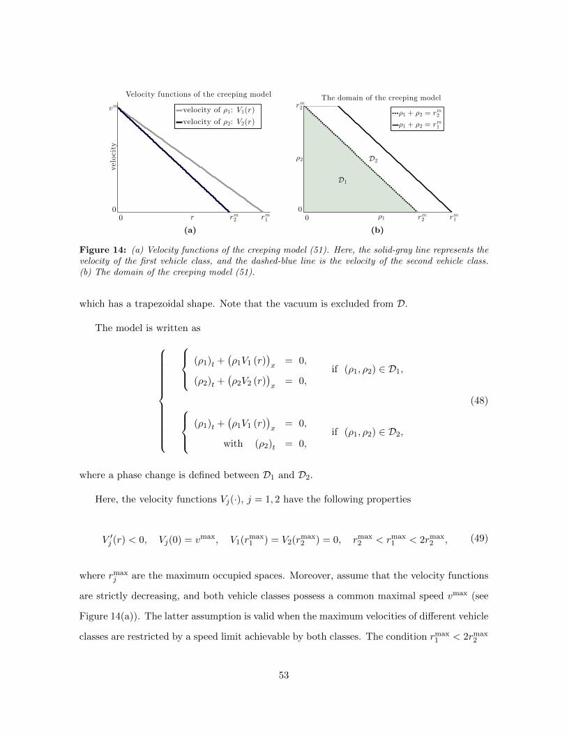
Velocity functions of the creeping model
vm
rm2 r
m1r
00
velocity
velocity of ρ1: V1(r)
velocity of ρ2: V2(r)
(a)
The domain of the creeping model
ρ2
rm
2
rm
2 rm
1ρ1
00
D2
D1
ρ1 + ρ2 = rm
2
ρ1 + ρ2 = rm
1
(b)
Figure 14: (a) Velocity functions of the creeping model (51). Here, the solid-gray line represents thevelocity of the first vehicle class, and the dashed-blue line is the velocity of the second vehicle class.(b) The domain of the creeping model (51).
which has a trapezoidal shape. Note that the vacuum is excluded from D.
The model is written as
(ρ1)t +(ρ1V1 (r)
)x
= 0,
(ρ2)t +(ρ2V2 (r)
)x
= 0,if (ρ1, ρ2) ∈ D1,
(ρ1)t +(ρ1V1 (r)
)x
= 0,
with (ρ2)t = 0,if (ρ1, ρ2) ∈ D2,
(48)
where a phase change is defined between D1 and D2.
Here, the velocity functions Vj(·), j = 1, 2 have the following properties
V ′j (r) < 0, Vj(0) = vmax, V1(rmax1 ) = V2(rmax
2 ) = 0, rmax2 < rmax
1 < 2rmax2 , (49)
where rmaxj are the maximum occupied spaces. Moreover, assume that the velocity functions
are strictly decreasing, and both vehicle classes possess a common maximal speed vmax (see
Figure 14(a)). The latter assumption is valid when the maximum velocities of different vehicle
classes are restricted by a speed limit achievable by both classes. The condition rmax1 < 2rmax
2
53
is a realistic condition on the maximum occupied space that simplifies the mathematical
analysis.
Remark 4. The phase transition models [6, 12, 13] apply a scalar conservation law in freeflow,
and a system of conservation laws in congestion. In the creeping model (51), a scalar model
is employed in the creeping phase, and a system of conservation laws is applied in the non-
creeping phase.
Based on the assumptions in (49), one may propose various velocity functions to gener-
ate multiclass fundamental diagrams, such as Drake’s exponential model, the smooth three-
parameter model [19], or Greenshields model [23]. Note that some of these models may
generate intersections between velocity curves for r > 0, which causes a loss of strict hyper-
bolicity away from the vacuum. This can be avoided depending on the choice of the free
parameters in each model. For simplicity, the linear Greenshields model is used:
V1(r) = vmax(1− r/rmax1 ), V2(r) = vmax(1− r/rmax
2 ). (50)
The model (48) with Greenshields velocity functions (50) is written as
(ρ1)t +(ρ1v
max(1− (ρ1 + ρ2)/rmax1 )
)x
= 0,
(ρ2)t +(ρ2v
max(1− (ρ1 + ρ2)/rmax2 )
)x
= 0,if (ρ1, ρ2) ∈ D1,
(ρ1)t +(ρ1v
max(1− (ρ1 + ρ2)/rmax1 )
)x
= 0,
with (ρ2)t = 0,if (ρ1, ρ2) ∈ D2.
(51)
By observing Figure 14(a), it is clear that the two velocity profiles only intersect at
the vacuum. As shown later, this simplifies the analysis of the creeping model compared to
intersections elsewhere in the domain. Because the velocity functions are linear, the deviation
between the two velocity functions strictly increases with r. Alternative velocity functions
may be considered to provide more control over the deviations and to potentially improve
the predictive capabilities of the model. Moreover, one sees that the Greenshields model (50)
54
generates a negative velocity for the second vehicle class for r > rmax2 . The creeping model
(51) successfully excludes the presence of this nonphysical negative velocity by applying a
phase transition.
Remark 5. Another approach one may consider to avoid negative velocity in the second vehicle
class while avoiding the need to pose the creeping model as a phase transition model is to
redefine the velocity function as
V2(r) =
V2(r), if r ≤ rmax2 ,
0, if rmax2 < r ≤ rmax
1 .
This approach is penalized by the loss of strict hyperbolicity for r > rmax2 .
Note that (51) also reduces to the LWR model in the sub-domain D3 = D1 ∩(ρ1 = 0 ∪
ρ2 = 0), when one vehicle class is absent. Accordingly, it is natural to use an LWR model
in D3, and to define phase transitions between D3 and other domains. However, this ap-
proach significantly increases the complexity in constructing Riemann solutions among dif-
ferent phases. Moreover, it is unnecessary since the creeping model (51) is strictly hyperbolic
in D1, and as shown in Section 3.4.4, it is consistent with the LWR model in D3.
3.4 Model Analysis
The ultimate goal of the analysis is to show that (51) is well-posed in D, and that the solution
is physically meaningful. In D2, the creeping model is rewritten as
(ρ1(x, t))t +(f1(ρ2(x), ρ1(x, t))
)x
= 0, (52)
where the flux function f1 = ρ1vmax(1 − (ρ1 + ρ2)/rmax
1 ) is smooth in ρ1 and ρ2, and ρ2(x)
is a bounded piecewise smooth function with a finite number of discontinuities. The well-
posedness of a scalar conservation law model in the form of (52) is established in [26, 27].
Thus, it remains to analyze the creeping model (51) in D1.
55
In D1, well-posedness of a system of conservation laws is shown in a general approach that
is based on constructing a solution to the Riemann problem for (51) with piecewise constant
initial data
u(x, 0) =
u+, if x > 0,
u−, if x < 0,(53)
where u− =(ρ−1 , ρ
−2
)and u+ =
(ρ+
1 , ρ+2
)are initial states. Based on the Riemann solver,
the existence theory follows from Glimm’s random choice method [21, 39] and the wavefront
tracking algorithm [1, 8, 9]. These techniques both require a strictly hyperbolic system of
conservation laws. As a result, a first and key issue is to establish the hyperbolicity of the
creeping model (51) in D1.
3.4.1 Hyperbolicity of the Creeping Model in D1
The conservation laws system in D1 is rewritten in a compact form
ut + f(u)x = 0,
where u = (ρ1, ρ2) is the vector of occupied space by class, and f =(ρ1V1(r), ρ2V2(r)
)is the
flux function. The Jacobian is calculated as
A = ∂f(u) =
V1 + α1 α1
α2 V2 + α2
, (54)
where α1 = ρ1V′
1 , and α2 = ρ2V′
2 . Strict hyperbolicity of (51) in D1 is established in the
following lemma.
Lemma 1. The creeping model (51) is strictly hyperbolic in D1.
Proof. The model is strictly hyperbolic if and only if the Jacobian has two distinct eigenvalues.
56
The characteristic polynomial of A is:
P (λ) = det (A− λI) = λ2 − (κ1 + κ2)λ+ κ1κ2 − α1α2,
where κj = vj + αj , and αj ≤ 0, j = 1, 2. It is easy to see that P always has two real roots
because
δ = (κ1 − κ2)2 + 4α1α2 ≥ 0,
thus, the system is hyperbolic. The only possibility to lose strict hyperbolicity is when δ = 0,
which occurs when α1 = 0 and V1 = κ2, or α2 = 0 and V2 = κ1. These conditions hold only
at the vacuum point, which does not belong to D1. Thus, λ1 and λ2 are distinct in D1, and
the creeping model (51) is strictly hyperbolic in D1.
Remark 6. Lemma 1 also holds for creeping models with velocity functions satisfying the
conditions in (49).
Furthermore, the characteristic speeds of (51) in D1 are
λ1 = 0.5(κ1 + κ2 −
√δ), λ2 = 0.5
(κ1 + κ2 +
√δ), (55)
where λ1 < λ2. The left and right eigenvectors associated to each eigenvalue λ are
`λ =
1V1−λ
1V2−λ
, γλ =
α1V1−λ
α2V2−λ
. (56)
The next lemma establishes that the creeping model (51) is anistropic.
Lemma 2. The characteristic speeds (55) are bounded above by the fastest vehicle class:
max λ1, λ2 ≤ max V1, V2 .
57
Proof. From (55) and the fact that αj ≤ 0, j = 1, 2, the bound for λ1 is given as
λ1 ≤ min κ1, κ2 ≤ min V1, V2 ≤ max V1, V2 .
For the second characteristic, one checks that
P(max κ1, κ2
)≤ 0, and P
(max V1, V2
)≥ 0.
By the intermediate value theorem, the bound for λ2 is established:
max κ1, κ2 ≤ λ2 ≤ max V1, V2 . (57)
Both λ1 and λ2 are bounded above by max V1, V2.
3.4.2 Property of the Characteristic Fields
Next, it is shown that the hyperbolic system (51) fits the Lax framework [31] in D1. This
is crucial for the construction of solutions to the Riemann problem, since it implies that the
Riemann solver consists of simple waves (or elementary waves). By the definition of Lax [31],
one needs to check that both characteristic fields(λ (u) , γλ (u)
)are either genuinely nonlinear
(∇λ (u) · γλ (u) 6= 0), or linearly degenerate (∇λ (u) · γλ (u) = 0) for all u in D1. Here, ∇λ
denotes the gradient of the function λ (u). The following lemma verifies that the creeping
model (51) is a Lax system in D1.
Lemma 3. Both characteristic fields of (51) are genuinely nonlinear in D1.
Proof. The proof follows the procedure outlined in [3]. Instead of evaluating ∇λ · γλ directly,
one defines ϕλ(γλ) as
ϕλ(γλ) = `λ · ∇2f(u) · (γλ, γλ) = (∇λ · γλ) (`λ · γλ) ,
58
and checks whether ϕλ(γλ) is non zero, since (`λ · γλ) 6= 0. One calculates ϕλ as
ϕλ(γλ) = vmax/rmax1 (λ− V2)
((γ
(1)λ
)2+ γ
(1)λ γ
(2)λ
)+ vmax/rmax
2 (λ− V1)
((γ
(2)λ
)2+ γ
(1)λ γ
(2)λ
),
where γ(1)λ and γ
(2)λ denote entries of the eigenvector γλ, i.e., γλ =
(γ
(1)λ , γ
(2)λ
).
For the slower characteristic λ1, it is clear that γ(1)λ1γ
(2)λ1≥ 0 for the eigenvector γλ1 in (56).
Moreover, from Lemma 2, one sees that ϕλ1 < 0 in D1. Thus, the first characteristic field is
genuinely nonlinear in D1.
For the faster characteristic λ2, ϕλ is rewritten as
ϕλ2(γλ2) = (γ(1)λ2
+ γ(2)λ2
)(vmax/rmax
1 γ(1)λ2
(λ2 − V2) + vmax/rmax2 γ
(2)λ2
(λ2 − V1)).
Thus, ϕλ2 vanishes if and only if
γ(1)λ2
+ γ(2)λ2
= 0, or vmax/rmax1 γ
(1)λ2
(λ2 − V2) + vmax/rmax2 γ
(2)λ2
(λ2 − V1) = 0. (58)
The first equality in (58) implies κ2 + α1 − κ1 − α2 = 0, which holds when V1 = V2. This
implies that the second characteristic is genuinely nonlinear except at the point where two
velocities coincide, i.e., at the vacuum.
Furthermore, the second equality of (58) gives
λ2 =κ2V1 + κ1V2
V1 + V2. (59)
Based on (57), it is clear that λ2 ≥ max κ1, κ2. In contrast, (59) implies
λ2 =κ2V1 + κ1V2
V1 + V2≤ max κ1, κ2 ,
so
λ2 =κ2V1 + κ1V2
V1 + V2= max κ1, κ2 . (60)
59
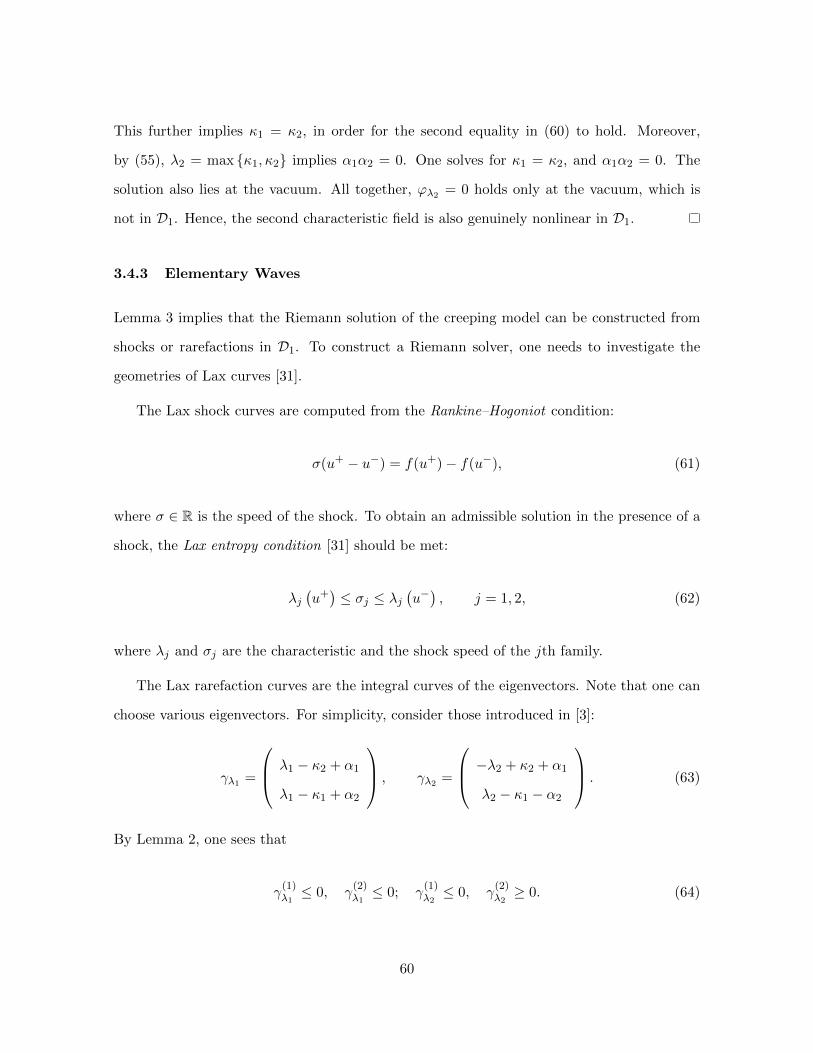
This further implies κ1 = κ2, in order for the second equality in (60) to hold. Moreover,
by (55), λ2 = max κ1, κ2 implies α1α2 = 0. One solves for κ1 = κ2, and α1α2 = 0. The
solution also lies at the vacuum. All together, ϕλ2 = 0 holds only at the vacuum, which is
not in D1. Hence, the second characteristic field is also genuinely nonlinear in D1.
3.4.3 Elementary Waves
Lemma 3 implies that the Riemann solution of the creeping model can be constructed from
shocks or rarefactions in D1. To construct a Riemann solver, one needs to investigate the
geometries of Lax curves [31].
The Lax shock curves are computed from the Rankine–Hogoniot condition:
σ(u+ − u−) = f(u+)− f(u−), (61)
where σ ∈ R is the speed of the shock. To obtain an admissible solution in the presence of a
shock, the Lax entropy condition [31] should be met:
λj(u+)≤ σj ≤ λj
(u−), j = 1, 2, (62)
where λj and σj are the characteristic and the shock speed of the jth family.
The Lax rarefaction curves are the integral curves of the eigenvectors. Note that one can
choose various eigenvectors. For simplicity, consider those introduced in [3]:
γλ1 =
λ1 − κ2 + α1
λ1 − κ1 + α2
, γλ2 =
−λ2 + κ2 + α1
λ2 − κ1 − α2
. (63)
By Lemma 2, one sees that
γ(1)λ1≤ 0, γ
(2)λ1≤ 0; γ
(1)λ2≤ 0, γ
(2)λ2≥ 0. (64)
60
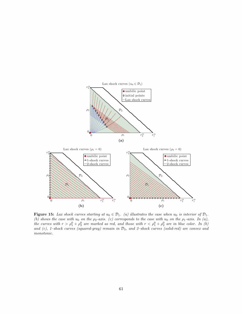
Lax shock curves (u0 ∈ D1)
rm
2
ρ2
rm
2 rm
1ρ1
00
D2
D1
umbilic point
initial points
Lax shock curves
(a)
Lax shock curves (ρ1 = 0)
rm
2
ρ2
rm
2ρ1 rm
1
00
D2
D1
umbilic point
1-shock curves2-shock curves
(b)
Lax shock curves (ρ2 = 0)
ρ2
rm
2
rm
2 rm
1ρ1
00
D2
D1
umbilic point
1-shock curves2-shock curves
(c)
Figure 15: Lax shock curves starting at u0 ∈ D1. (a) illustrates the case when u0 is interior of D1.(b) shows the case with u0 on the ρ2-axis. (c) corresponds to the case with u0 on the ρ1-axis. In (a),the curves with r > ρ01 + ρ02 are marked as red, and those with r < ρ01 + ρ02 are in blue color. In (b)and (c), 1–shock curves (squared-gray) remain in D3, and 2–shock curves (solid-red) are convex andmonotonic.
61
Geometry of the Lax Shock Curves From the Rankine–Hogoniot condition (61), Lax
shock curves starting from an initial state u0 = (ρ01, ρ
02) are
ρ1 (V1 − σ) = ρ01
(V 0
1 − σ), ρ2 (V2 − σ) = ρ0
2
(V 0
2 − σ), (65)
where V 01 = V1
(ρ0
1 + ρ02
)and V 0
2 = V2
(ρ0
1 + ρ02
). By solving for σ in the first equation of
(65), and substituting it into the second equation, (65) is rewritten as
ρ2
((ρ1 − ρ0
1)V2 −(ρ1V1 − ρ0
1V0
1
))= ρ0
2
((ρ1 − ρ0
1)V2 −(ρ1V1 − ρ0
1V0
1
)). (66)
Thus, Lax shock curves starting at u0 are represented as
H(u0) =
(ρ1, ρ2) ∈ R2 | s.t. (66) holds.
If u0 ∈ D1 \ D3, (66) is a hyperbola, which is convex and monotonic in the interior of D1.
Moreover, 1–shock curves are strictly increasing, while 2–shock curves are strictly decreasing
that exit from the ρ1-axis (see Figure 15(a)).
When u0 ∈ D3, e.g., on the ρ2-axis, (66) implies either ρ1 = 0, or σ = V1. In the former
case, (66) reduces to the Rankine–Hogoniot condition for an LWR model applied to the second
vehicle class. This is a 1–shock curve that coincides with the ρ2-axis. In the latter case, the
shock speed is the same as the velocity of the first vehicle class σ = V1. The hyperbola (66)
for 2–shock curves becomes
(rmax2 − rmax
1 ) ρ2 (ρ1 + ρ2)− rmax2 ρ0
2 (ρ1 + ρ2) + rmax1 ρ0
2
(ρ0
1 + ρ02
)= 0,
which is convex, monotonic, and exits from the boundary ρ2 = 0 (see Figure 15(b)). The
analysis of the case when u0 is on the ρ1-axis follows the same process, in which 1–shock
curves coincide with the ρ1-axis, and 2–shock curves are convex and monotonic, which exit
from the boundary ρ1 = 0 (see Figure 15(c)).
62
Geometry of the Lax Rarefaction Curves The lemma below gives the properties for
the Lax rarefaction curves.
Lemma 4. (i) the Lax rarefaction curves of (51) defined by (63) are monotonic and convex
in D1\D3; moreover (ii) the 1–rarefaction curves are monotonically increasing, while the
2–rarefaction curves are monotonically decreasing in D1\D3; and (iii) in D3, 1–rarefaction
curves coincide with the ρ1-axis and ρ2-axis. In contrast, 2–rarefaction curves only coincide
with the ρ2-axis.
Proof. First, the monotonicity of the Lax rarefaction curves follows from (64). To show the
concavity properties of the rarefaction curves, it is noted that the curvature of an integral
curve is positively proportional to γλj ∧ (∇γλj · γλj ) [3], where “ ∧ ” represents the exterior
product. One calculates that
γλj ∧ (∇γλj · γλj ) =2(a1 − a2)
(λj − V2)γ(1)λj
+ (λj − V1)γ(2)λj
(λj − V1)γ(1)λjγ
(2)λj
(γ
(1)λj
+ γ(2)λj
).
Here, aj = vmax/rmaxj , and a1 < a2 by (49). Moreover, one checks that in D1
γλj ∧ (∇γλj · γλj ) ≤ 0, j = 1, 2. (67)
By the definition of the eigenvectors (64), one sees the curvature center of each integral curve
lies above the integral curve, which implies that the rarefaction curves are convex.
Moreover, these curves have zero curvature if the equality in (67) holds:
γ(1)λj
+ γ(2)λj
= 0, or λj = V1, or γ(1)λj
= 0, or γ(2)λj
= 0. (68)
For the 1–rarefaction curves, the conditions in (68) are equivalent to
ρ1 = 0, ρ2 > 0, or ρ2 = 0, ρ1 > 0.
In other words, 1–rarefaction curves starting from a point in D3 remain in D3.
63
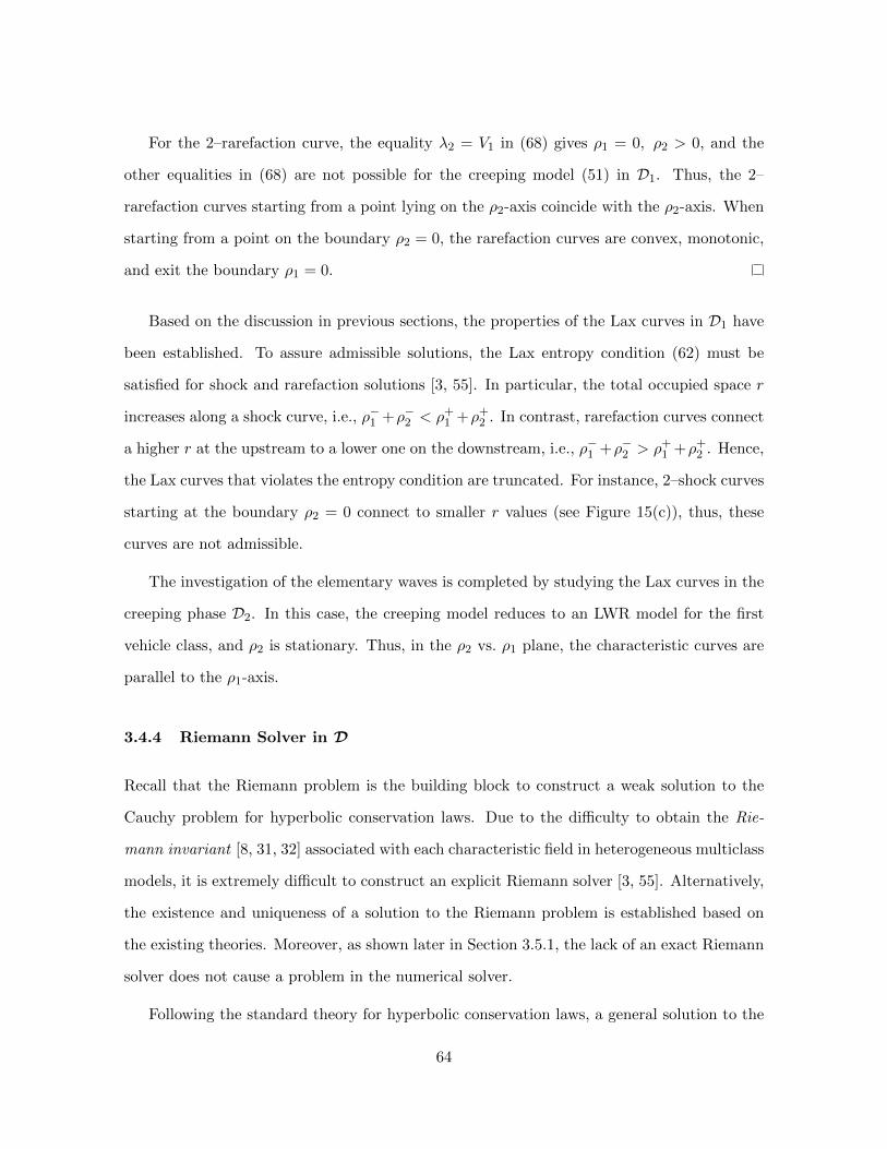
For the 2–rarefaction curve, the equality λ2 = V1 in (68) gives ρ1 = 0, ρ2 > 0, and the
other equalities in (68) are not possible for the creeping model (51) in D1. Thus, the 2–
rarefaction curves starting from a point lying on the ρ2-axis coincide with the ρ2-axis. When
starting from a point on the boundary ρ2 = 0, the rarefaction curves are convex, monotonic,
and exit the boundary ρ1 = 0.
Based on the discussion in previous sections, the properties of the Lax curves in D1 have
been established. To assure admissible solutions, the Lax entropy condition (62) must be
satisfied for shock and rarefaction solutions [3, 55]. In particular, the total occupied space r
increases along a shock curve, i.e., ρ−1 +ρ−2 < ρ+1 +ρ+
2 . In contrast, rarefaction curves connect
a higher r at the upstream to a lower one on the downstream, i.e., ρ−1 +ρ−2 > ρ+1 +ρ+
2 . Hence,
the Lax curves that violates the entropy condition are truncated. For instance, 2–shock curves
starting at the boundary ρ2 = 0 connect to smaller r values (see Figure 15(c)), thus, these
curves are not admissible.
The investigation of the elementary waves is completed by studying the Lax curves in the
creeping phase D2. In this case, the creeping model reduces to an LWR model for the first
vehicle class, and ρ2 is stationary. Thus, in the ρ2 vs. ρ1 plane, the characteristic curves are
parallel to the ρ1-axis.
3.4.4 Riemann Solver in D
Recall that the Riemann problem is the building block to construct a weak solution to the
Cauchy problem for hyperbolic conservation laws. Due to the difficulty to obtain the Rie-
mann invariant [8, 31, 32] associated with each characteristic field in heterogeneous multiclass
models, it is extremely difficult to construct an explicit Riemann solver [3, 55]. Alternatively,
the existence and uniqueness of a solution to the Riemann problem is established based on
the existing theories. Moreover, as shown later in Section 3.5.1, the lack of an exact Riemann
solver does not cause a problem in the numerical solver.
Following the standard theory for hyperbolic conservation laws, a general solution to the
64
Riemann problem with piecewise constant initial states (53) is defined by first connecting the
left state u− to an intermediate state u* with curves of the first family (1–Riemann invariant
is constant along 1–Lax curves), and then connecting u* to the right state u+ with curves of
the second family (2–Riemann invariant is constant along 2–Lax curves).
When both initial states are in D1, one constructs a unique Riemann solution based on
the structure of the Lax curves [31]. Here, it is important to verify that the solutions are
physically meaningful. In D3, an example that gives non-physical solutions is considered in the
n–populations model [3]. Given an initial condition with no vehicles of the second type, the
solution to the Riemann problem produces an intermediate state (ρ*1, ρ
*2) with the presence
of the second class, i.e., ρ*2 > 0. This is clearly incorrect because the second vehicle class
appears in the solution when initially it did not exist. The correct solution should be ρ*2 = 0,
and the Riemann solution should be consistent with the LWR model. The issue illustrated
in this example [3] is due to the loss of strict hyperbolicity in the n–populations model.
One verifies that the creeping model (51) is consistent with the LWR when only one vehicle
class is present. Based on the investigations of the geometry of Lax curves in Section 3.4.3,
1–Lax curves remain in D3. Therefore, it is clear that Riemann solutions are consistent with
those of the LWR model.
When u− and u+ are in D2, a Riemann problem for the LWR model is solved (see e.g.,
[36]). Thus, to complete the Riemann solver in D, it remains to define a solution for phase
transitions between D1 and D2. Consider the Riemann problem (53) with u− ∈ D2, and
u+ ∈ D1. In order to construct a Riemann solution with phase transition, one needs to find
intermediate states u∗ based on the elementary waves. Thus, a Riemann solution with two
intermediate states is defined:
1. A phase transition is defined by connecting u− = (ρ−1 , ρ−2 ) to the phase boundary
ρ1 + ρ2 = rmax2 along a curve that is parallel to the ρ1-axis. It is a rarefaction curve
in the conservation equation for the first vehicle class. This intermediate state can be
solved explicitly as u*1 = (rmax
2 − ρ−2 , ρ−2 ).
65
2. The second intermediate state u∗2 is constructed for a hyperbolic system with two initial
states u∗1, u+ ∈ D1.
The construction of a Riemann solution with u+ ∈ D2, and u− ∈ D1 follows the same
procedure.
3.4.5 Invariance of D
To guarantee a physical Riemann solution [2], one verifies that D (47) is an invariant region
for the Riemann problem. For convenience, the invariance of the two subdomains D1 and D2
is shown, and then the cases in the presence of a phase transition are considered.
First, it is easy to check that D1 is invariant since the creeping model (51) meets the
sufficient conditions proposed by Hoff [25].
Second, the domain D2 is invariant. This is because the Lax curves in D2 are parallel
to the ρ1-axis, and thus Riemann solution remains in D2 given both initial states in D2.
Finally, in the presence of a phase transition, the Riemann solution also remains in D (see
Section 3.4.4). It is concluded that D is invariant.
Remark 7. The invariance of D excludes the appearance of an intermediate vacuum state,
which exists for example in the ARZ model [2, 17].
By the Riemann solver described in Section 3.4.4, the Riemann solution always depends
continuously on the initial data, even with the presence of phase transitions. Therefore, it can
be verified that the size of the wave that connects two initial states∑
(u−, u+) of a Riemann
problem is bounded
c · ‖u+ − u−‖ ≤∑
(u−, u+) ≤ C · ‖u+ − u−‖, (69)
where c and C are given constants.
Next, the well-posedness of the Cauchy problem for the creeping model in D is established.
66
3.4.6 Cauchy Problem
Following the theories of phase transition models in [6, 12, 13], a weak solution to the Cauchy
problem of the system (51) is defined following a standard formulation. In particular, the
fluxes on the left and right states are defined when there is a phase change:
f− =
∑
j ρ−j Vj(ρ
−1 + ρ−2 ), if (ρ−1 , ρ
−2 ) ∈ D1
ρ−1 V1(ρ−1 + ρ−2 ), if (ρ−1 , ρ−2 ) ∈ D2
,
f+ =
∑
j ρ+j Vj(ρ
+1 + ρ+
2 ), if (ρ+1 , ρ
+2 ) ∈ D1
ρ+1 V1(ρ+
1 + ρ+2 ), if (ρ+
1 , ρ+2 ) ∈ D2
,
where the Rankine–Hogoniot condition (61) must be satisfied:
σ ·
∑j
ρ+j −
∑j
ρ−j
= f+ − f−.
The existence of an admissible solution to the Cauchy problem of the creeping model
(51) is proved by a standard wavefront tracking procedure [1, 8, 9]. Here, a sketch of the
proof is provided. Given a piecewise constant initial state with small total variation, the
front tracking algorithm defines a sequence of piecewise constant approximations (uk)k>1
by piecing together Riemann solutions at each interface where two fronts interact for each
time step. Based on (69), one sees that the total variation of uk(·, t) is bounded uniformly
for arbitrary initial states with small total variation. Finally, following the Glimm scheme
[21, 39], one can construct a subsequence of approximation solutions that converges to a
unique admissible weak solution, which depends continuously with initial data in D.
3.4.7 Vacuum Problem
The mathematical analysis of the previous sections is restricted to D, which excludes the
vacuum. In practice, vacuum initial states are physically meaningful, e.g., the downstream
of a red traffic light is empty. Thus, an appropriate model should define a solution to the
67
Riemann problem with an initial state or both initial states at the vacuum. The latter case
is trivial: the Riemann solution remains at the vacuum. The cases with only one initial state
at the vacuum are explored next.
Upstream Vacuum State One studies the Lax curves emanating from the vacuum u0 =
(0, 0). By the Rankine–Hogoniot condition:
ρ1 = 0, σ = V2 (ρ2) , or ρ2 = 0, σ = V1 (ρ1) .
These give 1–shock curves along the ρ2-axis, and 2–shock curves along the ρ1-axis.
Hence, in the case connecting the vacuum on the left to u+ ∈ D1, the shock solution first
connects to an intermediate state on the ρ2-axis with a 1–shock curve that coincides with the
ρ2-axis. A physical interpretation of this case is to consider a road with a queue of both large
and small vehicles at the downstream, and an empty road at the upstream. By the definition
of velocity function (see Figure 14(a)), the smaller vehicles possess a higher velocity for the
same total occupied space r. Thus, after a short period of time, only the larger vehicle class
ρ2 is observable at back of the queue because the first vehicle class overtakes them, i.e., ρ∗1 = 0
and ρ∗2 > 0. Therefore, starting from a vacuum state on the left, the Lax shock curves always
travel along the ρ2-axis and to connect with the slower class. Furthermore, one checks that
the shock speed of the 1–shock wave is the same as that predicted by the LWR model.
Downstream Vacuum State Based on the discussion in Section 3.4.3, 1–rarefaction
curves connect to the vacuum along the boundaries ρ1 = 0 and ρ2 = 0. Thus, the solu-
tion to the case with u− ∈ D3 is clear, where u− is connected with the vacuum along the
boundaries ρ1 = 0 and ρ2 = 0. It remains to discuss the case when u− ∈ D1\D3.
By the features of Lax rarefaction curves (see Section 3.4.3), 1–rarefaction curves are
monotonic, convex, and exit from the ρ2 = 0 boundary. Thus, u− first connects to an
intermediate state on the ρ1-axis via a 1–rarefaction curve. This also has clear physical
68
interpretation. As two vehicle classes flow into an empty road, the smaller vehicle class ρ1
advances to the front of the traffic, since it possesses higher speed for the same total occupied
space r (see Figure 14(a)). Thus, the intermediate state u∗ that connects to the vacuum at the
downstream contains only vehicles of the first class. Moreover, the u∗ and u+ are connected
along the ρ1-axis.
Riemann Solver at Vacuum The Riemann solver for the vacuum problem is summarized
as
Case 1: u− is at the vacuum (shock solution):
1. ρ+1 > 0, ρ+
2 > 0: It is a shock solution that connects u− to u∗ = (0, ρ∗2) by a 1–shock
curve along the boundary ρ1 = 0, with ρ+1 + ρ+
2 > ρ∗2 > ρ+2 , then connects u∗ and u+
with a 2–shock curve.
2. ρ+1 = 0, ρ+
2 > 0: The solution simplifies to a single 1–shock curve that connects u−
with u+ along the ρ2-axis.
3. ρ+1 > 0, ρ+
2 = 0: The intermediate state u∗ coincides with the vacuum. Hence, u− and
u+ are connected by a 2–shock curve along the ρ1-axis.
Case 2: u+ is at the vacuum (rarefaction solution):
1. ρ−1 > 0, ρ−2 > 0: In this case, the intermediate state appears on the ρ1-axis, i.e.,
u∗ = (ρ∗1, 0) with ρ−1 + ρ−2 > ρ∗1 > 0. Thus, the Riemann solution first links u− and u∗
with 1–rarefaction, and then to connect u∗ and the vacuum state along the ρ1-axis.
2. ρ−1 = 0, ρ−2 > 0, or ρ−1 > 0, ρ−2 = 0: The left state u− connects to the vacuum on the
right hand side directly via 1–rarefaction curves.
Case 3: both initial states are at the vacuum: Solution remains at the vacuum.
69
Stability Near the Vacuum The stability of the Riemann solver with initial data near
the vacuum is briefly discussed. Riemann solutions are constructed for a left state perturbed
away from the vacuum, and a fixed right state.
1. u− is perturbed to the ρ2-axis, ρ−1 = 0, 1 ρ−2 > 0: The Riemann solution is composed
of a 1–shock curve that connects u− to u* = (0, ρ*2) with ρ+
1 + ρ+2 > ρ*
2 > ρ−2 along the
ρ2-axis, and then a 2–shock curve that connects u* to u+.
2. u− is perturbed into the interior of D1, i.e., u− ∈ D1\D3, 1 ρ−1 > 0, 1 ρ−2 > 0: In
this case, the 1–shock curve is slightly shifted away from the ρ2-axis. The structure of
the solver is similar to the previous case, and the deviation between these two solutions
is small.
3. u− is perturbed to the ρ1-axis, 1 ρ−1 > 0, ρ−2 = 0: It gives an intermediate state
u* = (ρ*1, 0) with ρ*
1 > ρ+1 + ρ+
2 . First, u− connects to u∗ along a 1–shock curve that
coincides with the ρ1-axis. Second, u* connects to u+ via a 2–rarefaction curve.
In the third case, the 1–shock wave has a larger amplitude than the previous two cases,
and the 2–shock wave is replaced by a 2–rarefaction wave. Thus, the structure of the Riemann
solution changes for a small perturbation of the Riemann data. This may result in a loss of the
continuous dependence on the initial data. Consequently, it is possible to lose well-posedness
when the vacuum is involved. Due to the difficulty to obtain explicit solutions to the Riemann
problems, the well-posedness of the creeping model in the presence of the vacuum problem is
an open question.
70
3.5 Numerical Simulations
3.5.1 Numerical Method
This section is devoted to illustrate the creeping model (51) in numerical simulations, using
the Godunov method [22, 36]. The update rule is given explicitly as
ρk+11,i
ρk+12,i
=
ρk1,i
ρk2,i
− ∆t
∆x
(F1)ki+ 1
2
(F2)ki+ 12
− (F1)ki− 1
2
(F2)ki− 12
, (70)
where ∆x and ∆t are sizes of the space and time step, and ρkj,i represents the density of the
jth class in the ith cell at time t = k∆t. Moreover, (Fj)ki− 1
2and (Fj)
ki+ 1
2are numerical fluxes
through the upstream and downstream boundaries of the ith cell for the jth vehicle class at
time t = k∆t. These fluxes are obtained by explicitly analyzing the sending and receiving
potential for each vehicle class as an analogy to the CTM [14]. In [40], a generalization of
the CTM to homogeneous multiclass models is proposed. Here, a scheme for heterogeneous
extension of CTM is developed.
In the CTM framework, the flow is the minimum of sending and receiving functions, where
the sending function defines the number of vehicles available to be sent from upstream, and
the receiving function describes the number of vehicles available to be received downstream.
For simplicity, the initial states of upstream and downstream cells are represented as u− =
(ρ−1 , ρ−2 ) and u+ = (ρ+
1 , ρ+2 ). The flows of the two vehicle classes through the cell interface
are determined as
F1 = minS1(ρ−1 , ρ
−2 ), R1(ρ+
1 , ρ+2 ), F2 = min
S2(ρ−1 , ρ
−2 ), R2(ρ+
1 , ρ+2 ), (71)
where Sj(·) and Rj(·), j = 1, 2 represent the sending and receiving functions of the two vehicle
classes.
71
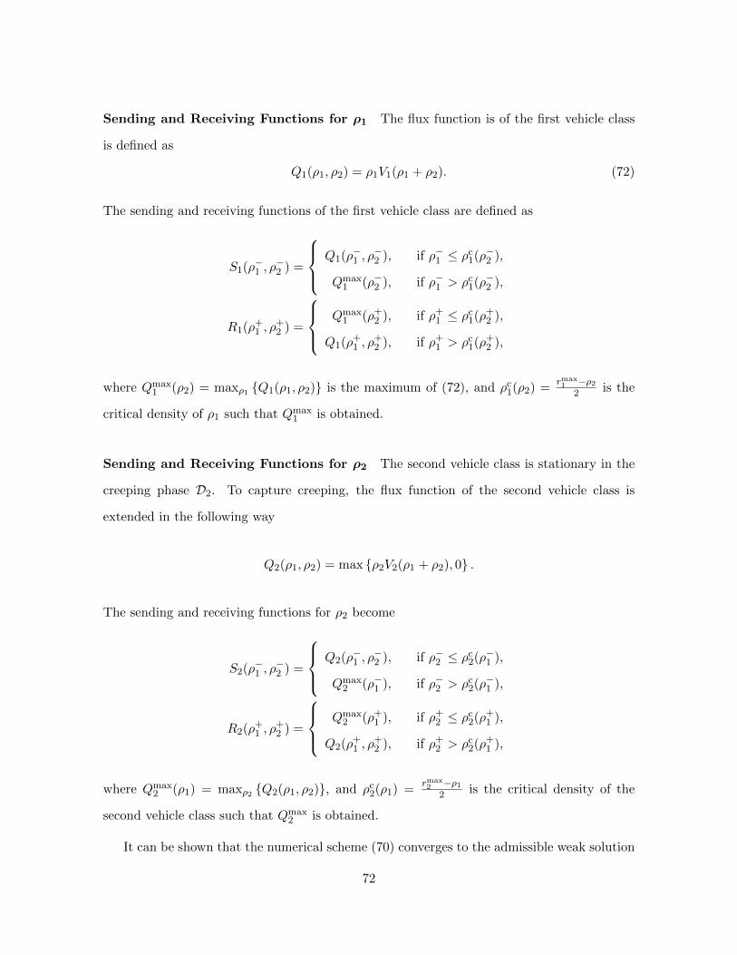
Sending and Receiving Functions for ρ1 The flux function is of the first vehicle class
is defined as
Q1(ρ1, ρ2) = ρ1V1(ρ1 + ρ2). (72)
The sending and receiving functions of the first vehicle class are defined as
S1(ρ−1 , ρ−2 ) =
Q1(ρ−1 , ρ−2 ), if ρ−1 ≤ ρc
1(ρ−2 ),
Qmax1 (ρ−2 ), if ρ−1 > ρc
1(ρ−2 ),
R1(ρ+1 , ρ
+2 ) =
Qmax1 (ρ+
2 ), if ρ+1 ≤ ρc
1(ρ+2 ),
Q1(ρ+1 , ρ
+2 ), if ρ+
1 > ρc1(ρ+
2 ),
where Qmax1 (ρ2) = maxρ1 Q1(ρ1, ρ2) is the maximum of (72), and ρc
1(ρ2) =rmax1 −ρ2
2 is the
critical density of ρ1 such that Qmax1 is obtained.
Sending and Receiving Functions for ρ2 The second vehicle class is stationary in the
creeping phase D2. To capture creeping, the flux function of the second vehicle class is
extended in the following way
Q2(ρ1, ρ2) = max ρ2V2(ρ1 + ρ2), 0 .
The sending and receiving functions for ρ2 become
S2(ρ−1 , ρ−2 ) =
Q2(ρ−1 , ρ−2 ), if ρ−2 ≤ ρc
2(ρ−1 ),
Qmax2 (ρ−1 ), if ρ−2 > ρc
2(ρ−1 ),
R2(ρ+1 , ρ
+2 ) =
Qmax2 (ρ+
1 ), if ρ+2 ≤ ρc
2(ρ+1 ),
Q2(ρ+1 , ρ
+2 ), if ρ+
2 > ρc2(ρ+
1 ),
where Qmax2 (ρ1) = maxρ2 Q2(ρ1, ρ2), and ρc
2(ρ1) =rmax2 −ρ1
2 is the critical density of the
second vehicle class such that Qmax2 is obtained.
It can be shown that the numerical scheme (70) converges to the admissible weak solution
72
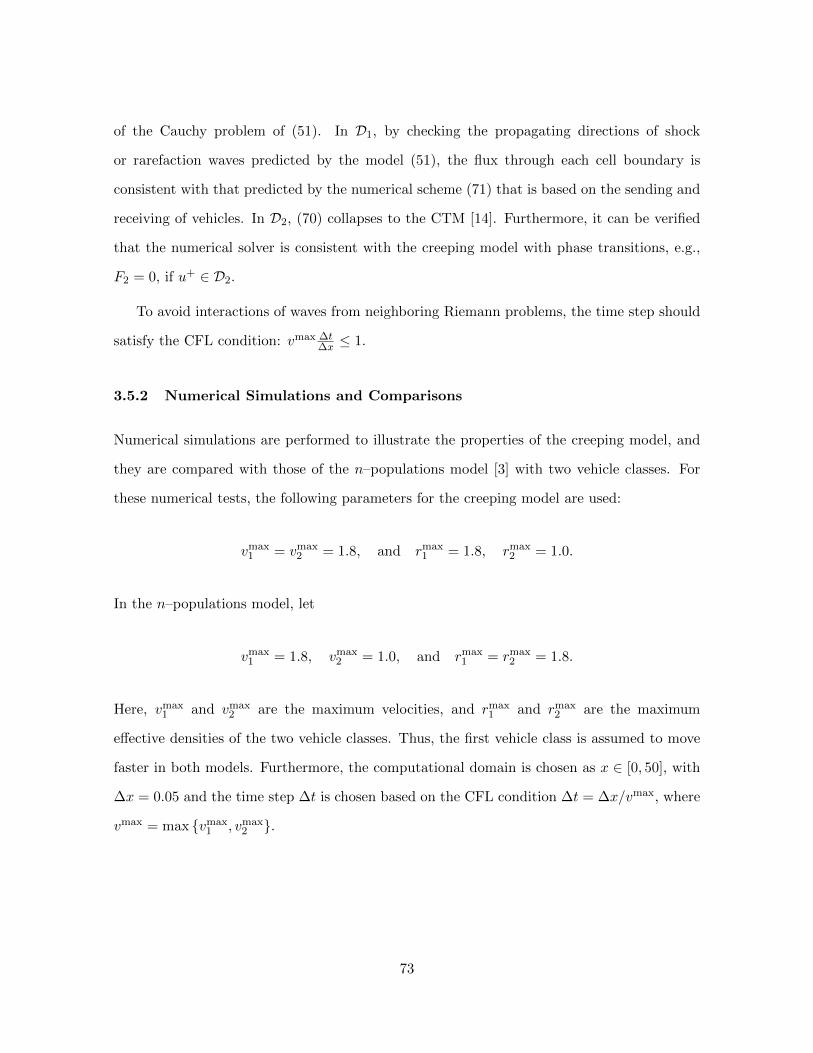
of the Cauchy problem of (51). In D1, by checking the propagating directions of shock
or rarefaction waves predicted by the model (51), the flux through each cell boundary is
consistent with that predicted by the numerical scheme (71) that is based on the sending and
receiving of vehicles. In D2, (70) collapses to the CTM [14]. Furthermore, it can be verified
that the numerical solver is consistent with the creeping model with phase transitions, e.g.,
F2 = 0, if u+ ∈ D2.
To avoid interactions of waves from neighboring Riemann problems, the time step should
satisfy the CFL condition: vmax ∆t∆x ≤ 1.
3.5.2 Numerical Simulations and Comparisons
Numerical simulations are performed to illustrate the properties of the creeping model, and
they are compared with those of the n–populations model [3] with two vehicle classes. For
these numerical tests, the following parameters for the creeping model are used:
vmax1 = vmax
2 = 1.8, and rmax1 = 1.8, rmax
2 = 1.0.
In the n–populations model, let
vmax1 = 1.8, vmax
2 = 1.0, and rmax1 = rmax
2 = 1.8.
Here, vmax1 and vmax
2 are the maximum velocities, and rmax1 and rmax
2 are the maximum
effective densities of the two vehicle classes. Thus, the first vehicle class is assumed to move
faster in both models. Furthermore, the computational domain is chosen as x ∈ [0, 50], with
∆x = 0.05 and the time step ∆t is chosen based on the CFL condition ∆t = ∆x/vmax, where
vmax = max vmax1 , vmax
2 .
73
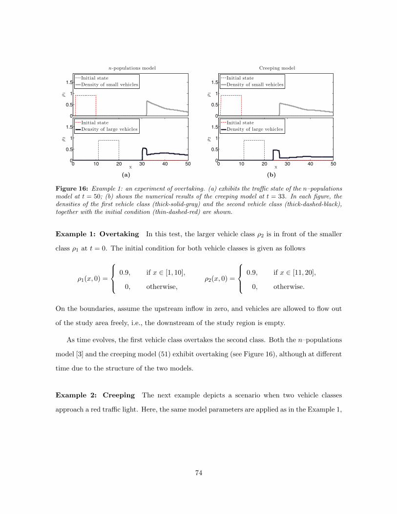
0
0.5
1
1.5
n-populations modelρ1
Initial state
Density of small vehicles
0 10 20 30 40 500
0.5
1
1.5
x
ρ2
Initial state
Density of large vehicles
(a)
0
0.5
1
1.5
Creeping model
ρ1
Initial state
Density of small vehicles
0 10 20 30 40 500
0.5
1
1.5
x
ρ2
Initial state
Density of large vehicles
(b)
Figure 16: Example 1: an experiment of overtaking. (a) exhibits the traffic state of the n–populationsmodel at t = 50; (b) shows the numerical results of the creeping model at t = 33. In each figure, thedensities of the first vehicle class (thick-solid-gray) and the second vehicle class (thick-dashed-black),together with the initial condition (thin-dashed-red) are shown.
Example 1: Overtaking In this test, the larger vehicle class ρ2 is in front of the smaller
class ρ1 at t = 0. The initial condition for both vehicle classes is given as follows
ρ1(x, 0) =
0.9, if x ∈ [1, 10],
0, otherwise,ρ2(x, 0) =
0.9, if x ∈ [11, 20],
0, otherwise.
On the boundaries, assume the upstream inflow in zero, and vehicles are allowed to flow out
of the study area freely, i.e., the downstream of the study region is empty.
As time evolves, the first vehicle class overtakes the second class. Both the n–populations
model [3] and the creeping model (51) exhibit overtaking (see Figure 16), although at different
time due to the structure of the two models.
Example 2: Creeping The next example depicts a scenario when two vehicle classes
approach a red traffic light. Here, the same model parameters are applied as in the Example 1,
74
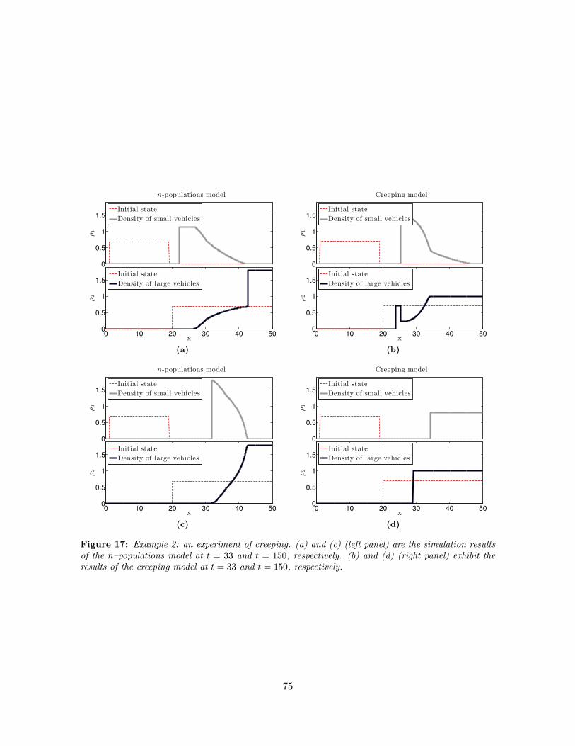
0
0.5
1
1.5
n-populations model
ρ1
Initial state
Density of small vehicles
0 10 20 30 40 500
0.5
1
1.5
x
ρ2
Initial state
Density of large vehicles
(a)
0
0.5
1
1.5
Creeping model
ρ1
Initial state
Density of small vehicles
0 10 20 30 40 500
0.5
1
1.5
x
ρ2
Initial state
Density of large vehicles
(b)
0
0.5
1
1.5
n-populations model
ρ1
Initial state
Density of small vehicles
0 10 20 30 40 500
0.5
1
1.5
x
ρ2
Initial state
Density of large vehicles
(c)
0
0.5
1
1.5
Creeping model
ρ1
Initial state
Density of small vehicles
0 10 20 30 40 500
0.5
1
1.5
x
ρ2
Initial state
Density of large vehicles
(d)
Figure 17: Example 2: an experiment of creeping. (a) and (c) (left panel) are the simulation resultsof the n–populations model at t = 33 and t = 150, respectively. (b) and (d) (right panel) exhibit theresults of the creeping model at t = 33 and t = 150, respectively.
75
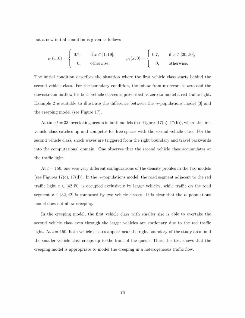
but a new initial condition is given as follows
ρ1(x, 0) =
0.7, if x ∈ [1, 19],
0, otherwise,ρ2(x, 0) =
0.7, if x ∈ [20, 50],
0, otherwise.
The initial condition describes the situation where the first vehicle class starts behind the
second vehicle class. For the boundary condition, the inflow from upstream is zero and the
downstream outflow for both vehicle classes is prescribed as zero to model a red traffic light.
Example 2 is suitable to illustrate the difference between the n–populations model [3] and
the creeping model (see Figure 17).
At time t = 33, overtaking occurs in both models (see Figures 17(a), 17(b)), where the first
vehicle class catches up and competes for free spaces with the second vehicle class. For the
second vehicle class, shock waves are triggered from the right boundary and travel backwards
into the computational domain. One observes that the second vehicle class accumulates at
the traffic light.
At t = 150, one sees very different configurations of the density profiles in the two models
(see Figures 17(c), 17(d)). In the n–populations model, the road segment adjacent to the red
traffic light x ∈ [42, 50] is occupied exclusively by larger vehicles, while traffic on the road
segment x ∈ [32, 42] is composed by two vehicle classes. It is clear that the n–populations
model does not allow creeping.
In the creeping model, the first vehicle class with smaller size is able to overtake the
second vehicle class even through the larger vehicles are stationary due to the red traffic
light. At t = 150, both vehicle classes appear near the right boundary of the study area, and
the smaller vehicle class creeps up to the front of the queue. Thus, this test shows that the
creeping model is appropriate to model the creeping in a heterogeneous traffic flow.
76
4 Conclusion
In this work, the joint traffic state estimation and incident detection problem is formulated as
a hybrid state estimation problem. A second order traffic flow model with incident dynamics
is implemented with a MMPF to solve the estimation problem in simulation, using traffic
incident data generated from CORSIM. Compared to a particle filter applied to a second
order traffic flow model with time-invariant parameters, the new algorithm can significantly
improve traffic estimates while also estimating the location and severity of incidents.
Next, a new heterogeneous model for two vehicle classes is developed, which is based on
the philosophy that vehicles with different sizes occupy different spaces on the roadway. The
model is designed to capture the creeping scenario when large vehicles are stopped, while
smaller vehicles continue to move. To achieve this goal, velocity functions are introduced
that have the same maximum velocity but distinct maximum occupied spaces. The model is
described as a phase transition model where a 2 × 2 system reduces to the LWR model as
the occupied space increases above a critical point rmax2 . A Riemann solver is defined across
the phase transition. Finally, numerical tests based on finite volume Godunov scheme are
performed, and comparisons between creeping model and the two class n–populations model
are carried out. These tests show that the creeping model can not only describe overtaking
behavior, but also model the dynamics of creeping in heterogeneous flow.
77
References
[1] F. Ancona and A. Marson. Existence theory by front tracking for general nonlinear
hyperbolic systems. Archive for rational mechanics and analysis, 185(2):287–340, 2007.
[2] A. Aw and M. Rascle. Resurrection of second order models of traffic flow. SIAM J. Appl.
Math., 60:916–944, 2000.
[3] S. Benzoni-Gavage and R. M. Colombo. An n-populations model for traffic flow. European
Journal of Applied Mathematics, 14(5):587–612, 2003.
[4] F. Berthelin, P. Degond, M. Delitala, and M. Rascle. A model for the formation and
evolution of traffic jams. Arch. Ration. Mech. Anal., 187:185–220, 2008.
[5] S. Blandin, J. Argote, A. Bayen, and D. Work. Phase transition model of non-stationary
traffic flow: definition, properties and solution methods. Transportation Research Part
B, 52(2013):31–55, 2013.
[6] S. Blandin, D. Work, P. Goatin, B. Piccoli, and A. Bayen. A general phase transition
model for vehicular traffic. SIAM J. Appl. Math., 71(1):107–127, 2011.
[7] A. P. Blom, Henk and Y. Bar-Shalom. The interacting multiple model algorithm for
systems with markovian switching coefficients. IEEE Transactions on Automatic Control,
33(8):780–783, 1988.
[8] A. Bressan. Hyperbolic systems of conservation laws – The one dimensional Cauchy
problem. Oxford University Press, Oxford, 2000.
[9] A. Bressan and R. M. Colombo. The semigroup generated by 2× 2 conservation laws.
Archive for rational mechanics and analysis, 133(1):1–75, 1995.
[10] G. Bretti, R. Natalini, and B. Piccoli. A fluid-dynamic traffic model on road networks.
Archives of Computational Methods in Engineering, 14(2):139–172, 2007.
78
[11] G. M. Coclite, M. Garavello, and B. Piccoli. Traffic flow on a road network. SIAM J.
Math. Anal., 36(6):1862–1886, 2005.
[12] R. M. Colombo. Hyperbolic phase transitions in traffic flow. SIAM Journal on Applied
Mathematics, 63(2):708–721, 2003.
[13] R. M. Colombo, P. Goatin, and F. S. Priuli. Global well posedness of traffic flow
models with phase transitions. Nonlinear Analysis: Theory, Methods & Applications,
66(11):2413–2426, 2007.
[14] C. F. Daganzo. The cell transmission model: A dynamic representation of highway traffic
consistent with the hydrodynamic theory. Transportation Research Part B: Methodolog-
ical, 28(4):269–287, 1994.
[15] C. F. Daganzo. A continuum theory of traffic dynamics for freeways with special lanes.
Transportation Research Part B: Methodological, 31(2):83–102, 1997.
[16] C. F. Daganzo. A behavioral theory of multi-lane traffic flow. part i: Long homogeneous
freeway sections. Transportation Research Part B: Methodological, 36(2):131–158, 2002.
[17] S. Fan, M. Herty, and B. Seibold. Comparative model accuracy of a data-fitted general-
ized Aw-Rascle-Zhang model. Netw. Heterog. Media, Vol. 9, No. 2:239–268, 2014.
[18] S. Fan, B. Piccoli, and B. Seibold. A collapsed generalized Aw-Rascle-Zhang model.
SIAM J. Appl. Math., In process.
[19] S. Fan and B. Seibold. A comparison of data-fitted first order traffic models and their
second order generalizations via trajectory and sensor data. 93rd Annual Meeting of
Transportation Research Board, Washington DC, 2013. paper number 13–4853.
[20] M. Garavello and B. Piccoli. Traffic flow on a road network using the aw–rascle model.
Communications in Partial Differential Equations, 31(2):243–275, 2006.
[21] J. Glimm. Solutions in the large for nonlinear hyperbolic systems of equations. Commu-
nications on Pure and Applied Mathematics, 18(4):697–715, 1965.
79
[22] S. K. Godunov. A difference scheme for the numerical computation of a discontinuous
solution of the hydrodynamic equations. Math. Sbornik, 47:271–306, 1959.
[23] B. D. Greenshields. A study of traffic capacity. Proceedings of the Highway Research
Record, 14:448–477, 1935.
[24] M. Herty and M. Rascle. Coupling conditions for a class of second order models for
traffic flow. SIAM J. Math. Anal., 38(2):595–616, 2006.
[25] D. Hoff. Invariant regions for systems of conservation laws. Transactions of the American
Mathematical Society, 289(2):591–610, 1985.
[26] K. H. Karlsen, N. H. Risebro, and J. Towers. Upwind difference approximations for de-
generate parabolic convection–diffusion equations with a discontinuous coefficient. IMA
J. Numer. Anal., 22(4):623–664, 2002.
[27] K. H. Karlsen, N. H. Risebro, and J. Towers. L1 stability for entropy solutions of nonlin-
ear degenerate parabolic convection-diffusion equations with discontinuous coefficients.
Skr. K. Nor. Vid. Selsk, 2003.
[28] B. S. Kerner. Experimental features of the emergence of moving jams in free traffic flow.
J. Phys. A, 33:221–228, 2000.
[29] B. S. Kerner. Phase transitions in traffic flow. Traffic and Granular Flow. Springer,
2000.
[30] B. L. Keyfitz and H. C. Kranzer. A system of non-strictly hyperbolic conservation laws
arising in elasticity theory. Archive for Rational Mechanics and Analysis, 72(3):219–241,
1980.
[31] P. D. Lax. Hyperbolic systems of conservation laws II. Communications on Pure and
Applied Mathematics, 10(4):537–566, 1957.
[32] P. G. Le Floch. Hyperbolic Systems of Conservation Laws: The theory of classical and
nonclassical shock waves. Birkhauser, 2002.
80
[33] J. P. Lebacque. The Godunov scheme and what it means for first order traffic flow
models. In 13th International Symposium on Transportation and Traffic Theory, pages
647–677, 1996.
[34] J. P. Lebacque, S. Mammar, and H. Haj-Salem. Generic second order traffic flow mod-
elling. In R. E. Allsop, M. G. H. Bell, and B. G. Heydecker, editors, Transportation and
Traffic Theory, Proc. of the 17th ISTTT, pages 755–776. Elsevier, 2007.
[35] J. P. Lebacque and Salim Mammar. Second order traffic flow modeling: supply-demand
analysis of the inhomogeneous riemann problem and of boundary conditions.
[36] R. J. LeVeque. Finite volume methods for hyperbolic problems. Cambridge University
Press, 2002.
[37] X. R. Li and V. P. Jilkov. Survey of maneuvering target tracking. part v. multiple-model
methods. IEEE Transactions on Aerospace and Electronic Systems, 41(4):1255–1321,
2005.
[38] M.J. Lighthill and G.B. Whitham. On kinematic waves II. a theory of traffic flow on
long crowded roads. Proceedings of the Royal Society of London. Series A. Mathematical
and Physical Sciences, 229(1178):317–345, 1955.
[39] T. P. Liu and T. Yang. Weak solutions of general systems of hyperbolic conservation
laws. Communications in mathematical physics, 230(2):289–327, 2002.
[40] S. Logghe and L. H. Immers. Heterogeneous traffic flow modelling with the LWR model
using passenger-car equivalents. In Proceedings of the 10th World congress on ITS,
Madrid (Spain), 2003.
[41] S. Logghe and L. H. Immers. Multi-class kinematic wave theory of traffic flow. Trans-
portation Research Part B: Methodological, 42(6):523–541, 2008.
[42] CORSIM Users Manual. FHWA. US Department of Transportation, Office of Safety and
Traffic Operations, 1997.
81
[43] Efim Mazor, Amir Averbuch, Yakov Bar-Shalom, and Joshua Dayan. Interacting multi-
ple model methods in target tracking: a survey. IEEE Transactions on Aerospace and
Electronic Systems, 34(1):103–123, 1998.
[44] R. Nair, H. S. Mahmassani, and E. Miller-Hooks. A porous flow approach to modeling
heterogeneous traffic in disordered systems. Transportation Research Part B: Method-
ological, 45(9):1331 – 1345, 2011.
[45] D. Ngoduy and R. Liu. Multiclass first-order simulation model to explain non-linear
traffic phenomena. Physica A: Statistical Mechanics and its Applications, 385(2):667–
682, 2007.
[46] P.I. Richards. Shock waves on the highway. Operation Research, 4(1):42–51, 1956.
[47] B. Ristic, S. Arulampalm, and N. Gordon. Beyond the Kalman filter: Particle filters for
tracking applications. Artech House Publishers, 2004.
[48] S. Smulders. Control of freeway traffic flow by variable speed signs. Transportation
Research Part B: Methodological, 24(2):111 – 132, 1990.
[49] S. Tafazoli and X. Sun. Hybrid system state tracking and fault detection using particle
filters. IEEE Transactions on Control Systems Technology, 14(6):1078–1087, 2006.
[50] J. W. C. Van Lint, S. P. Hoogendoorn, and M. Schreuder. Fastlane: New multiclass first-
order traffic flow model. Transportation Research Record: Journal of the Transportation
Research Board, 2088(1):177–187, 2008.
[51] R. Wang, D. B. Work, and R. Sowers. Multiple model particle smoothing for traffic inci-
dent detection. Submitted to IEEE Transactions on Intelligent Transportation Systems,
2004.
[52] G. C. K. Wong and S. C. Wong. A multi-class traffic flow model an extension of LWR
model with heterogeneous drivers. Transportation Research Part A: Policy and Practice,
36(9):827 – 841, 2002.
82
[53] H. M. Zhang. A non-equilibrium traffic model devoid of gas-like behavior. Transp. Res.
B, 36:275–290, 2002.
[54] H. M. Zhang and W. L. Jin. Kinematic wave traffic flow model for mixed traffic. Trans-
portation Research Record: Journal of the Transportation Research Board, 1802(1):197–
204, 2002.
[55] P. Zhang, R. X. Liu, S. C. Wong, and S. Q. Dai. Hyperbolicity and kinematic waves of
a class of multi-population partial differential equations. European Journal of Applied
Mathematics, 17(2):171–200, 2006.
[56] P. Zhang, S. C. Wong, and S. Q. Dai. A conserved higher-order anisotropic traffic flow
model: description of equilibrium and non-equilibrium flows. Transportation Research
Part B: Methodological, 43(5):562–574, 2009.
[57] Z. Zhu and T. Wu. Two-phase fluids model for freeway traffic flow and its application to
simulate evolution of solitons in traffic. Journal of transportation engineering, 129(1):51–
56, 2002.
83


![FLEXSYS Motion-based Traffic Analysis and … Traffic Analysis and Incident Detection ... Komatsu and Sasa [9] ... generates a qualitative description of the tra–c directly from](https://img.pdfslide.us/doc/110x75/5b49a38e7f8b9aa82c8b85fc/flexsys-motion-based-traffic-analysis-and-traffic-analysis-and-incident-detection.jpg)