Application of Control Volume Energy Balance for Analysing

Application of Control Volume Energy Balance for AnalysingPropeller-Hull Interaction in Presence of Free-surface

Downloaded from: https://research.chalmers.se, 2021-12-29 00:18 UTC

Citation for the original published paper (version of record):Eslamdoost, A., Andersson, J., Bensow, R. et al (2019)Application of Control Volume Energy Balance for Analysing Propeller-Hull Interaction inPresence of Free-surfaceSixth International Symposium on Marine Propulsors

N.B. When citing this work, cite the original published paper.

research.chalmers.se offers the possibility of retrieving research publications produced at Chalmers University of Technology.It covers all kind of research output: articles, dissertations, conference papers, reports etc. since 2004.research.chalmers.se is administrated and maintained by Chalmers Library

(article starts on next page)

Sixth International Symposium on Marine Propulsors SMP’19, Rome, Italy, May 2019

Application of Control Volume Energy Balance for Analysing

Propeller-Hull Interaction in Presence of Free-surface

Arash Eslamdoost1, Jennie Andersson1, Rickard Bensow1, Marko Vikström2

1Department of Mechanics and Maritime Sciences, Chalmers University of Technology, Gothenburg, Sweden 2Kongsberg Hydrodynamic Research Centre, Kristinehamn, Sweden

ABSTRACT Reynolds-Transport Theorem can be employed for analysing the conservation of energy equation over a control volume. Through this approach we can decompose the propeller delivered power into mechanical and thermal energy components. This approach not only enables us to qualitatively describe the flow but also makes it possible to quantify different energy flux components and understand the energy loss mechanisms within the studied system. Employing this method, the effect of free-surface on propeller-hull interaction is studied for an axisymmetric body in the vicinity of free-surface relative to a deeply submerged body. The required flow quantities for the control volume analysis are obtained from a Reynolds-Averaged Navier-Stokes approach together with a Volume-of-Fluid method for capturing the free-surface. The mechanical and thermal energy flux components have been computed for control volumes of different sizes, even including the free-surface. These results deviate less than 0.5% from the propeller delivered power which verifies the applicability of the method for further analysis of the interaction effects. The self-propelled hull is studied in two different depths and thus the propeller loadings and efficiencies are different. The analysis of energy flux components quantitatively explains the reasons for the differences. Keywords propeller-hull interaction, free-surface, Reynolds-Averaged Navier-Stokes, energy equation 1 INTRODUCTION The interaction effects between propeller and hull are important design factors. The performance of the entire system can be improved noticeably by considering the interaction effects during the propeller and hull design process. These effects are most commonly described using a well-established terminology, including thrust deduction, wake fraction, propulsive efficiency etc. However, this approach does not provide much information on the interaction details. Several attempts have been made to develop methods and guidelines based on analytical or CFD approaches for analysing the interaction effects by identifying the energy losses in the system. Some of them are based on potential flow assumptions, for instance, Dyne and Jonsson (1989) and Dyne (1995), and some are based on viscous flow analysis, e.g. van Terwisga (2013), Schuiling et al. (2016,

2018), Eslamdoost et al. (2017) and Andersson et al. (2018 a, 2018b, 2018c). Grounded on Reynolds Transport Theorem for energy, these papers study the energy flux through control volumes enclosing propeller or entire propeller-hull system, which provides a quantitative approach for decomposing the shaft power into different change of energy components inside the outlined control volume. Identifying energy fluxes through a control volume provides a series of extra detailed information on the flow to better understand the propeller-hull interaction effects. Although the control volume analysis of momentum flux for studying wave making and viscous resistance of ships in presence of free-surface have been discussed extensively (see for instance Morenoet al (1975); Dyne and Lindell (1994); Faltinsen (2005); Molland et al (2011)), it is very difficult to find studies which discuss control volume analysis of energy flux for ships including free-surface. To reduce the aforementioned knowledge gap, the objective of the current paper is to evaluate the feasibility of employing the Reynolds Transport Theorem for energy over control volumes including free-surface. In order to avoid unnecessary flow complexities, a simple axisymmetric body with a standard propeller is studied with and without free-surface. In case of free-surface presence, the hull is submerged one body diameter below the undisturbed water level. A Reynolds-Averaged Navier-Stokes (RANS) approach is used for computing the flow field. Based on the calculated flow field, all energy flux components through different control volumes around the propeller and hull are obtained and used for investigating the propeller-hull interaction effects. 2 CONTROL VOLUME APPROACH FOR ENERGY ANALYSIS We can keep track of the total energy delivered to the system (propeller work) through the energy components and their conversion from one form to another. This can be done with the aid of the Reynolds Transport Theorem. This theorem states that the rate of change of an extensive property (here total energy, E), for the system is equal to the time rate of change of that property within the control volume plus the net flux rate of the property through the control surface. Conventionally propeller’s delivered power is obtained through its torque and rotation rate,


𝑃" = 2𝜋𝑛𝑄, (1)

where 𝑛 is the shaft revolution per second and 𝑄 is the shaft torque.

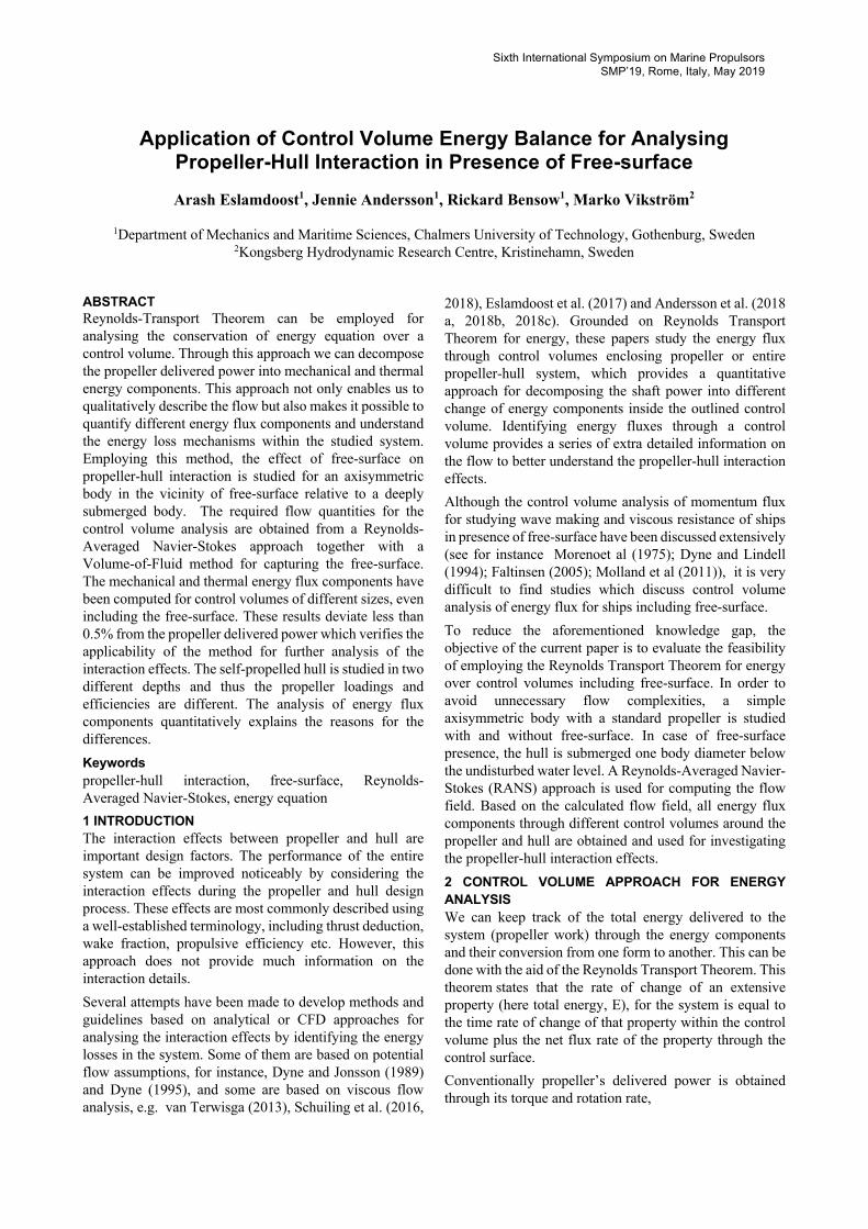
Figure 1. A sample cylindrical control volume around the axisymmetric body and the propeller.

Alternatively, one may use Reynolds Transport Theorem for a control volume enclosing the propulsion system (see Figure 1) for obtaining the delivered power, as shown in Equation (2).

𝑃" = )12𝑢,

-𝜌(𝑢0⃗ ∙ 𝑛0⃗ )45

𝑑 + )128𝑢9

- + 𝑢:-;𝜌(𝑢0⃗ ∙ 𝑛0⃗ )45

𝑑𝑆

+ ) 𝑘𝜌(𝑢0⃗ ∙ 𝑛0⃗ )45

𝑑𝑆 + ) 𝑝(𝑢0⃗ ∙ 𝑛0⃗ )45

𝑑𝑆 + ) 𝑢@𝜌(𝑢0⃗ ∙ 𝑛0⃗ )45

𝑑𝑆,

(2)

where 𝑘 is the turbulent kinetic energy and 𝑢,, 𝑢9 and 𝑢: are the axial, radial and the tangential velocity components, respectively. The control surfaces are denoted by 𝐶𝑆. The first four terms on the right-hand side are the axial kinetic energy, the transversal kinetic energy, the turbulent kinetic energy and the work done by pressure forces, respectively. The effect of gravitational acceleration can be neglected if the hydrodynamic pressure is used in the pressure work term. The fifth term on the right-hand side of Equation (2) represents the internal energy change within the control volume, which can be obtained through,

𝑢@ = 𝑐C𝑇, (3) where 𝑐C is the specific heat of the fluid and 𝑇 is temperature. In a viscous flow, kinetic energy of the mean flow is converted to internal energy, i.e. heat, either through dissipation of turbulent velocity fluctuations or direct viscous dissipation from the mean flow. The internal energy flux accounts for both these processes, whereas the turbulent kinetic energy flux only accounts for an intermediate stage in the process of turbulent kinetic energy dissipation. The latter term has to be included only due to the CFD modeling, where an eddy-viscosity model is used for turbulence modeling. In summary, the above-mentioned energy balance method shows that the delivered power of a propeller can be balanced with a set of different energy flux components through control surfaces of a deliberate control volume enclosing the system. Thus, the system performance can be

studied more in detail by analyzing different energy flux components through the control surfaces. 3 COMPUTATIONAL METHOD, DOMAIN AND MESH We have employed the commercial CFD package STAR-CCM+13.06, a finite volume method solver, in this study. The code solves the conservation equations for momentum, mass, turbulence quantities as well as energy using a segregated solver based on the SIMPLE-algorithm. A 2nd order upwind discretization scheme in space was used. We have solved the energy equation, to be able to measure the dissipation of kinetic energy and turbulent kinetic energy in the form of an increased temperature (Equation (3)). The turbulence was modeled using a RANS approach and the k-ω SST model. The tracing of free-surface is done using the Volume of Fluid method (VOF) in combination with the High-Resolution Interface Capturing (HRIC) scheme to discretize the convective term of the volume fraction transport equation (Muzaferija & Perić, 1999). This scheme is suitable for tracking sharp interphase of an immiscible phase mixture and resolves the free-surface within typically one cell. All the aforementioned equations were solved employing an implicit unsteady solver. In order to estimate the propeller rotation rate a Moving Reference Frame (MRF) technique was used to find thrust-resistance balance. Then, when the forces are stabilized, a Rigid Body Motion (RBM) technique is triggered which solves the actual propeller rotation. The time step used with RBM is equivalent to the time for 1 degree of propeller rotation. The propeller rotation rate is fine-adjusted to consider for the slightly different thrust obtained with RBM in comparison to MRF.

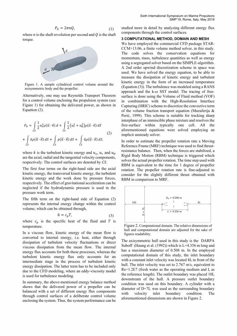
Figure 2. Computational domain. The relative dimensions of hull and computational domain are adjusted for the sake of figures readability.

The axisymmetric hull used in this study is the DARPA Suboff (Haung et al. (1992)) which is L=4.356 m long and has a maximum diameter of 0.508 m. In the employed computational domain of this study, the inlet boundary with a constant inlet velocity was located 4L in front of the hull. The inlet velocity was set to 2.767 m/s, equivalent to Re=1.2E7 (fresh water as the operating medium and L as the reference length). The outlet boundary was placed 10L downstream of the hull. A pressure outlet boundary condition was used on this boundary. A cylinder with a diameter of D=7L was used as the surrounding boundary with velocity inlet boundary condition. The aforementioned dimensions are shown in Figure 2.

!

!

!" = 0.508)

* = 4.356)

4*10*

!=7L


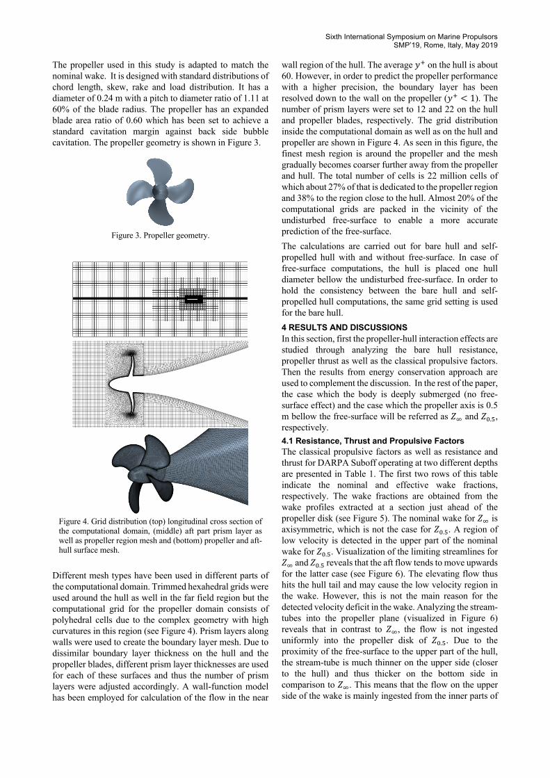
The propeller used in this study is adapted to match the nominal wake. It is designed with standard distributions of chord length, skew, rake and load distribution. It has a diameter of 0.24 m with a pitch to diameter ratio of 1.11 at 60% of the blade radius. The propeller has an expanded blade area ratio of 0.60 which has been set to achieve a standard cavitation margin against back side bubble cavitation. The propeller geometry is shown in Figure 3.

Figure 3. Propeller geometry.

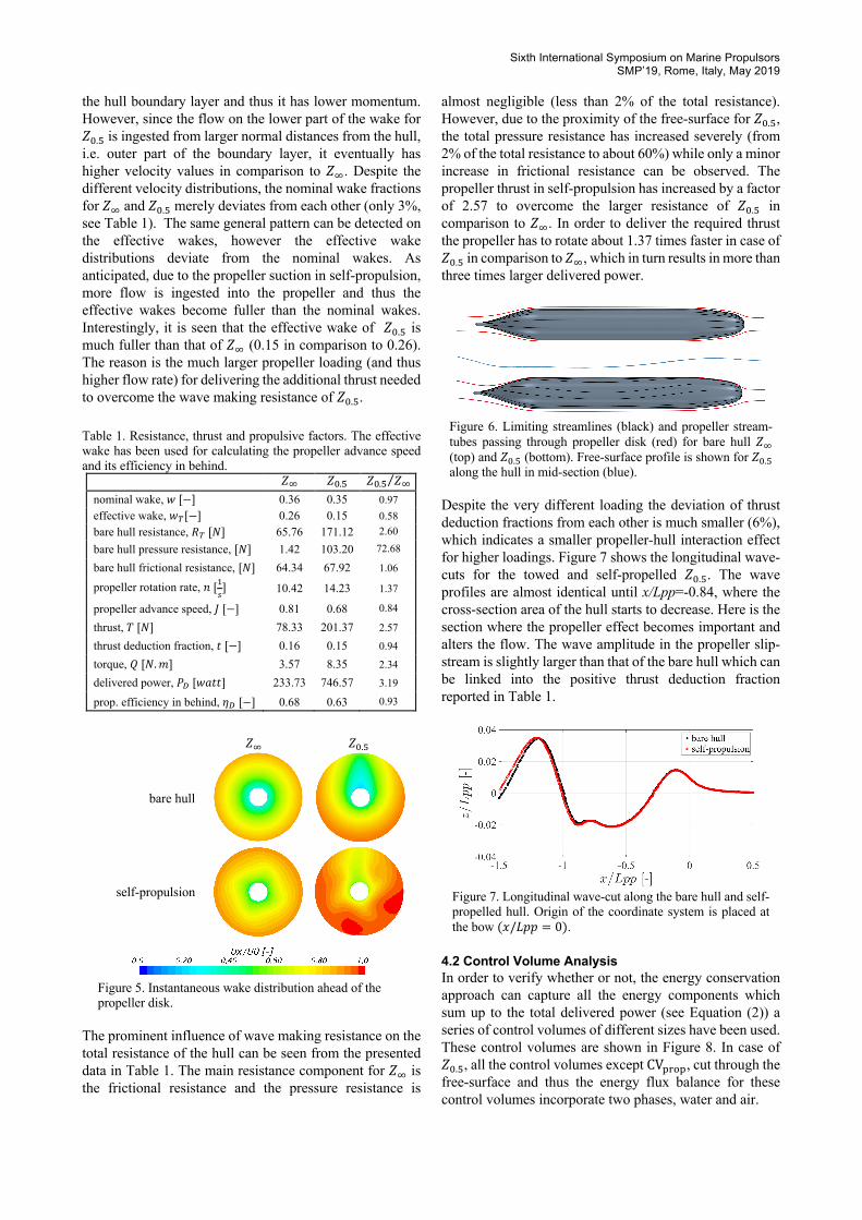
Figure 4. Grid distribution (top) longitudinal cross section of the computational domain, (middle) aft part prism layer as well as propeller region mesh and (bottom) propeller and aft-hull surface mesh.

Different mesh types have been used in different parts of the computational domain. Trimmed hexahedral grids were used around the hull as well in the far field region but the computational grid for the propeller domain consists of polyhedral cells due to the complex geometry with high curvatures in this region (see Figure 4). Prism layers along walls were used to create the boundary layer mesh. Due to dissimilar boundary layer thickness on the hull and the propeller blades, different prism layer thicknesses are used for each of these surfaces and thus the number of prism layers were adjusted accordingly. A wall-function model has been employed for calculation of the flow in the near

wall region of the hull. The average 𝑦H on the hull is about 60. However, in order to predict the propeller performance with a higher precision, the boundary layer has been resolved down to the wall on the propeller (𝑦H < 1). The number of prism layers were set to 12 and 22 on the hull and propeller blades, respectively. The grid distribution inside the computational domain as well as on the hull and propeller are shown in Figure 4. As seen in this figure, the finest mesh region is around the propeller and the mesh gradually becomes coarser further away from the propeller and hull. The total number of cells is 22 million cells of which about 27% of that is dedicated to the propeller region and 38% to the region close to the hull. Almost 20% of the computational grids are packed in the vicinity of the undisturbed free-surface to enable a more accurate prediction of the free-surface. The calculations are carried out for bare hull and self-propelled hull with and without free-surface. In case of free-surface computations, the hull is placed one hull diameter bellow the undisturbed free-surface. In order to hold the consistency between the bare hull and self-propelled hull computations, the same grid setting is used for the bare hull. 4 RESULTS AND DISCUSSIONS In this section, first the propeller-hull interaction effects are studied through analyzing the bare hull resistance, propeller thrust as well as the classical propulsive factors. Then the results from energy conservation approach are used to complement the discussion. In the rest of the paper, the case which the body is deeply submerged (no free-surface effect) and the case which the propeller axis is 0.5 m bellow the free-surface will be referred as 𝑍K and 𝑍L.N, respectively. 4.1 Resistance, Thrust and Propulsive Factors The classical propulsive factors as well as resistance and thrust for DARPA Suboff operating at two different depths are presented in Table 1. The first two rows of this table indicate the nominal and effective wake fractions, respectively. The wake fractions are obtained from the wake profiles extracted at a section just ahead of the propeller disk (see Figure 5). The nominal wake for 𝑍K is axisymmetric, which is not the case for 𝑍L.N. A region of low velocity is detected in the upper part of the nominal wake for 𝑍L.N. Visualization of the limiting streamlines for 𝑍K and 𝑍L.N reveals that the aft flow tends to move upwards for the latter case (see Figure 6). The elevating flow thus hits the hull tail and may cause the low velocity region in the wake. However, this is not the main reason for the detected velocity deficit in the wake. Analyzing the stream-tubes into the propeller plane (visualized in Figure 6) reveals that in contrast to 𝑍K, the flow is not ingested uniformly into the propeller disk of 𝑍L.N. Due to the proximity of the free-surface to the upper part of the hull, the stream-tube is much thinner on the upper side (closer to the hull) and thus thicker on the bottom side in comparison to 𝑍K. This means that the flow on the upper side of the wake is mainly ingested from the inner parts of


the hull boundary layer and thus it has lower momentum. However, since the flow on the lower part of the wake for 𝑍L.N is ingested from larger normal distances from the hull, i.e. outer part of the boundary layer, it eventually has higher velocity values in comparison to 𝑍K. Despite the different velocity distributions, the nominal wake fractions for 𝑍K and 𝑍L.N merely deviates from each other (only 3%, see Table 1). The same general pattern can be detected on the effective wakes, however the effective wake distributions deviate from the nominal wakes. As anticipated, due to the propeller suction in self-propulsion, more flow is ingested into the propeller and thus the effective wakes become fuller than the nominal wakes. Interestingly, it is seen that the effective wake of 𝑍L.N is much fuller than that of 𝑍K (0.15 in comparison to 0.26). The reason is the much larger propeller loading (and thus higher flow rate) for delivering the additional thrust needed to overcome the wave making resistance of 𝑍L.N. Table 1. Resistance, thrust and propulsive factors. The effective wake has been used for calculating the propeller advance speed and its efficiency in behind.

𝑍K 𝑍L.N

bare hull

self-propulsion

Figure 5. Instantaneous wake distribution ahead of the propeller disk.

The prominent influence of wave making resistance on the total resistance of the hull can be seen from the presented data in Table 1. The main resistance component for 𝑍K is the frictional resistance and the pressure resistance is

almost negligible (less than 2% of the total resistance). However, due to the proximity of the free-surface for 𝑍L.N, the total pressure resistance has increased severely (from 2% of the total resistance to about 60%) while only a minor increase in frictional resistance can be observed. The propeller thrust in self-propulsion has increased by a factor of 2.57 to overcome the larger resistance of 𝑍L.N in comparison to 𝑍K. In order to deliver the required thrust the propeller has to rotate about 1.37 times faster in case of 𝑍L.N in comparison to 𝑍K, which in turn results in more than three times larger delivered power.

Figure 6. Limiting streamlines (black) and propeller stream-tubes passing through propeller disk (red) for bare hull 𝑍K (top) and 𝑍L.N (bottom). Free-surface profile is shown for 𝑍L.N along the hull in mid-section (blue).

Despite the very different loading the deviation of thrust deduction fractions from each other is much smaller (6%), which indicates a smaller propeller-hull interaction effect for higher loadings. Figure 7 shows the longitudinal wave-cuts for the towed and self-propelled 𝑍L.N. The wave profiles are almost identical until x/Lpp=-0.84, where the cross-section area of the hull starts to decrease. Here is the section where the propeller effect becomes important and alters the flow. The wave amplitude in the propeller slip-stream is slightly larger than that of the bare hull which can be linked into the positive thrust deduction fraction reported in Table 1.

Figure 7. Longitudinal wave-cut along the bare hull and self-propelled hull. Origin of the coordinate system is placed at the bow (𝑥/𝐿𝑝𝑝 = 0).

4.2 Control Volume Analysis In order to verify whether or not, the energy conservation approach can capture all the energy components which sum up to the total delivered power (see Equation (2)) a series of control volumes of different sizes have been used. These control volumes are shown in Figure 8. In case of 𝑍L.N, all the control volumes except CVUVWU, cut through the free-surface and thus the energy flux balance for these control volumes incorporate two phases, water and air.

!" !#.% !#.% !"⁄ nominal wake, '[−] 0.36 0.35 0.97 effective wake, ',[−] 0.26 0.15 0.58 bare hull resistance, -,[.] 65.76 171.12 2.60

bare hull pressure resistance, [.] 1.42 103.20 72.68

bare hull frictional resistance, [.] 64.34 67.92 1.06

propeller rotation rate, /[01] 10.42 14.23 1.37

propeller advance speed, 2[−] 0.81 0.68 0.84

thrust, 3[.] 78.33 201.37 2.57

thrust deduction fraction, 4[−] 0.16 0.15 0.94

torque, 5[..6] 3.57 8.35 2.34

delivered power, 78['944] 233.73 746.57 3.19

prop. efficiency in behind, :8[−] 0.68 0.63 0.93


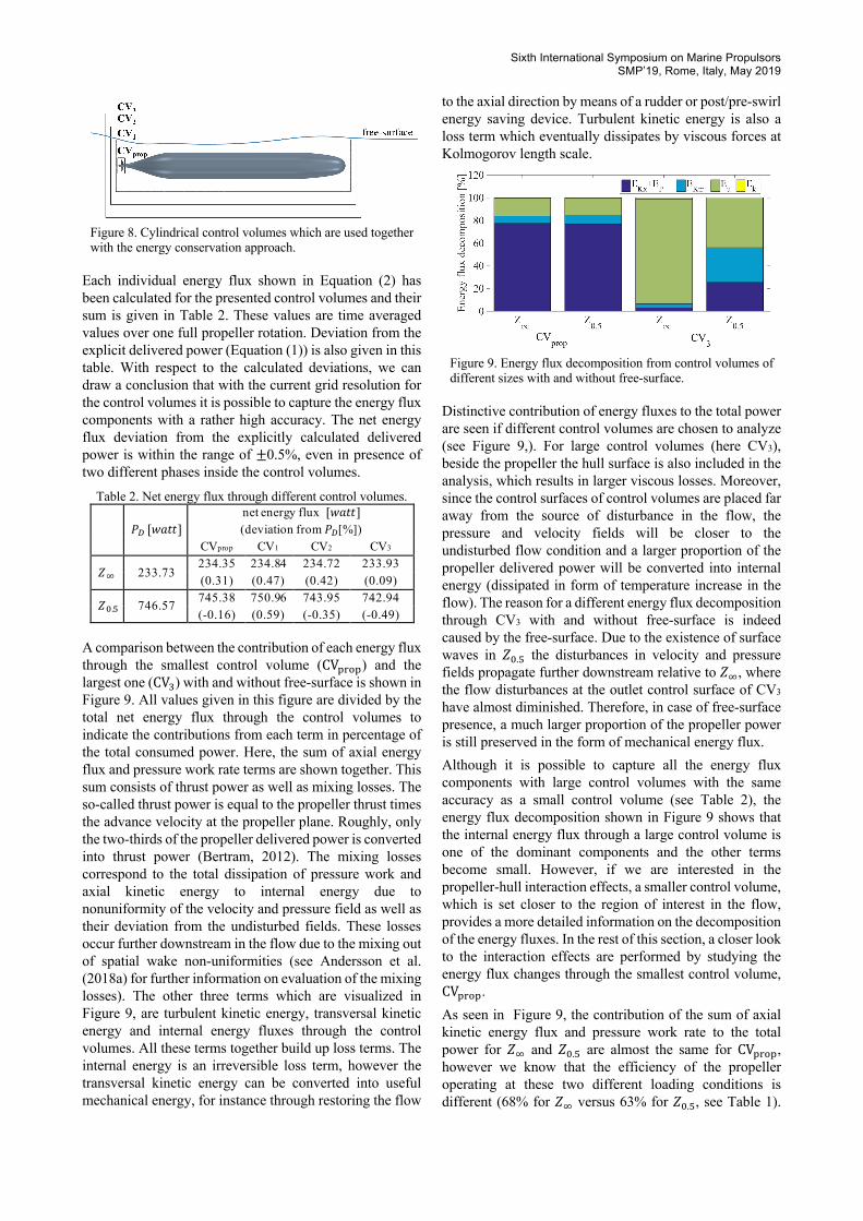
Figure 8. Cylindrical control volumes which are used together with the energy conservation approach.

Each individual energy flux shown in Equation (2) has been calculated for the presented control volumes and their sum is given in Table 2. These values are time averaged values over one full propeller rotation. Deviation from the explicit delivered power (Equation (1)) is also given in this table. With respect to the calculated deviations, we can draw a conclusion that with the current grid resolution for the control volumes it is possible to capture the energy flux components with a rather high accuracy. The net energy flux deviation from the explicitly calculated delivered power is within the range of ±0.5%, even in presence of two different phases inside the control volumes.

Table 2. Net energy flux through different control volumes.

A comparison between the contribution of each energy flux through the smallest control volume (CVUVWU) and the largest one (CVY) with and without free-surface is shown in Figure 9. All values given in this figure are divided by the total net energy flux through the control volumes to indicate the contributions from each term in percentage of the total consumed power. Here, the sum of axial energy flux and pressure work rate terms are shown together. This sum consists of thrust power as well as mixing losses. The so-called thrust power is equal to the propeller thrust times the advance velocity at the propeller plane. Roughly, only the two-thirds of the propeller delivered power is converted into thrust power (Bertram, 2012). The mixing losses correspond to the total dissipation of pressure work and axial kinetic energy to internal energy due to nonuniformity of the velocity and pressure field as well as their deviation from the undisturbed fields. These losses occur further downstream in the flow due to the mixing out of spatial wake non-uniformities (see Andersson et al. (2018a) for further information on evaluation of the mixing losses). The other three terms which are visualized in Figure 9, are turbulent kinetic energy, transversal kinetic energy and internal energy fluxes through the control volumes. All these terms together build up loss terms. The internal energy is an irreversible loss term, however the transversal kinetic energy can be converted into useful mechanical energy, for instance through restoring the flow

to the axial direction by means of a rudder or post/pre-swirl energy saving device. Turbulent kinetic energy is also a loss term which eventually dissipates by viscous forces at Kolmogorov length scale.

Figure 9. Energy flux decomposition from control volumes of different sizes with and without free-surface.

Distinctive contribution of energy fluxes to the total power are seen if different control volumes are chosen to analyze (see Figure 9,). For large control volumes (here CV3), beside the propeller the hull surface is also included in the analysis, which results in larger viscous losses. Moreover, since the control surfaces of control volumes are placed far away from the source of disturbance in the flow, the pressure and velocity fields will be closer to the undisturbed flow condition and a larger proportion of the propeller delivered power will be converted into internal energy (dissipated in form of temperature increase in the flow). The reason for a different energy flux decomposition through CV3 with and without free-surface is indeed caused by the free-surface. Due to the existence of surface waves in 𝑍L.N the disturbances in velocity and pressure fields propagate further downstream relative to 𝑍K, where the flow disturbances at the outlet control surface of CV3 have almost diminished. Therefore, in case of free-surface presence, a much larger proportion of the propeller power is still preserved in the form of mechanical energy flux. Although it is possible to capture all the energy flux components with large control volumes with the same accuracy as a small control volume (see Table 2), the energy flux decomposition shown in Figure 9 shows that the internal energy flux through a large control volume is one of the dominant components and the other terms become small. However, if we are interested in the propeller-hull interaction effects, a smaller control volume, which is set closer to the region of interest in the flow, provides a more detailed information on the decomposition of the energy fluxes. In the rest of this section, a closer look to the interaction effects are performed by studying the energy flux changes through the smallest control volume, CVUVWU. As seen in Figure 9, the contribution of the sum of axial kinetic energy flux and pressure work rate to the total power for 𝑍K and 𝑍L.N are almost the same for CVUVWU, however we know that the efficiency of the propeller operating at these two different loading conditions is different (68% for 𝑍K versus 63% for 𝑍L.N, see Table 1).

!"[%&'']

net energy flux [%&''] (deviation from !"[%])

CVprop CV1 CV2 CV3

)* 233.73 234.35 234.84 234.72 233.93 (0.31) (0.47) (0.42) (0.09)

)+.- 746.57 745.38 750.96 743.95 742.94 (-0.16) (0.59) (-0.35) (-0.49)


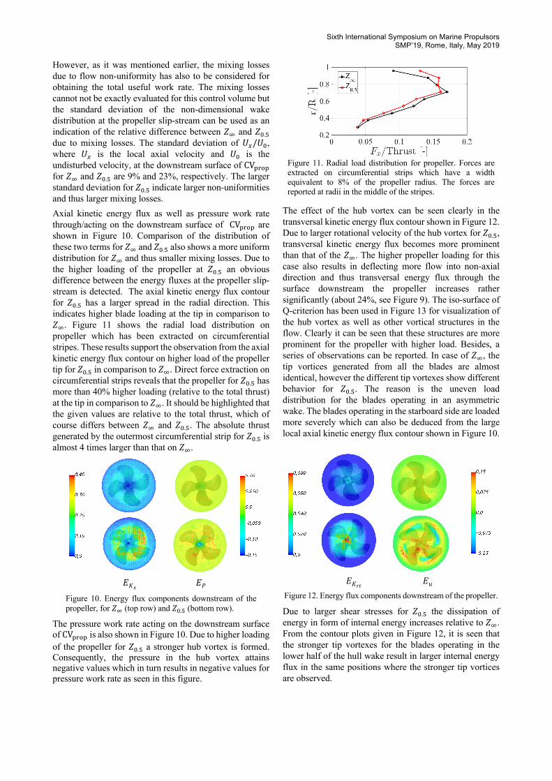
However, as it was mentioned earlier, the mixing losses due to flow non-uniformity has also to be considered for obtaining the total useful work rate. The mixing losses cannot not be exactly evaluated for this control volume but the standard deviation of the non-dimensional wake distribution at the propeller slip-stream can be used as an indication of the relative difference between 𝑍K and 𝑍L.N due to mixing losses. The standard deviation of 𝑈,/𝑈L, where 𝑈, is the local axial velocity and 𝑈L is the undisturbed velocity, at the downstream surface of CVUVWU for 𝑍K and 𝑍L.N are 9% and 23%, respectively. The larger standard deviation for 𝑍L.N indicate larger non-uniformities and thus larger mixing losses. Axial kinetic energy flux as well as pressure work rate through/acting on the downstream surface of CVUVWU are shown in Figure 10. Comparison of the distribution of these two terms for 𝑍K and 𝑍L.N also shows a more uniform distribution for 𝑍K and thus smaller mixing losses. Due to the higher loading of the propeller at 𝑍L.N an obvious difference between the energy fluxes at the propeller slip-stream is detected. The axial kinetic energy flux contour for 𝑍L.N has a larger spread in the radial direction. This indicates higher blade loading at the tip in comparison to 𝑍K. Figure 11 shows the radial load distribution on propeller which has been extracted on circumferential stripes. These results support the observation from the axial kinetic energy flux contour on higher load of the propeller tip for 𝑍L.N in comparison to 𝑍K. Direct force extraction on circumferential strips reveals that the propeller for 𝑍L.N has more than 40% higher loading (relative to the total thrust) at the tip in comparison to 𝑍K. It should be highlighted that the given values are relative to the total thrust, which of course differs between 𝑍K and 𝑍L.N. The absolute thrust generated by the outermost circumferential strip for 𝑍L.N is almost 4 times larger than that on 𝑍K.

𝐸𝐾𝑥 𝐸𝑃

Figure 10. Energy flux components downstream of the propeller, for 𝑍K (top row) and 𝑍L.N (bottom row).

The pressure work rate acting on the downstream surface of CVUVWU is also shown in Figure 10. Due to higher loading of the propeller for 𝑍L.N a stronger hub vortex is formed. Consequently, the pressure in the hub vortex attains negative values which in turn results in negative values for pressure work rate as seen in this figure.

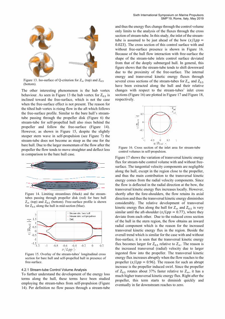
Figure 11. Radial load distribution for propeller. Forces are extracted on circumferential strips which have a width equivalent to 8% of the propeller radius. The forces are reported at radii in the middle of the stripes.

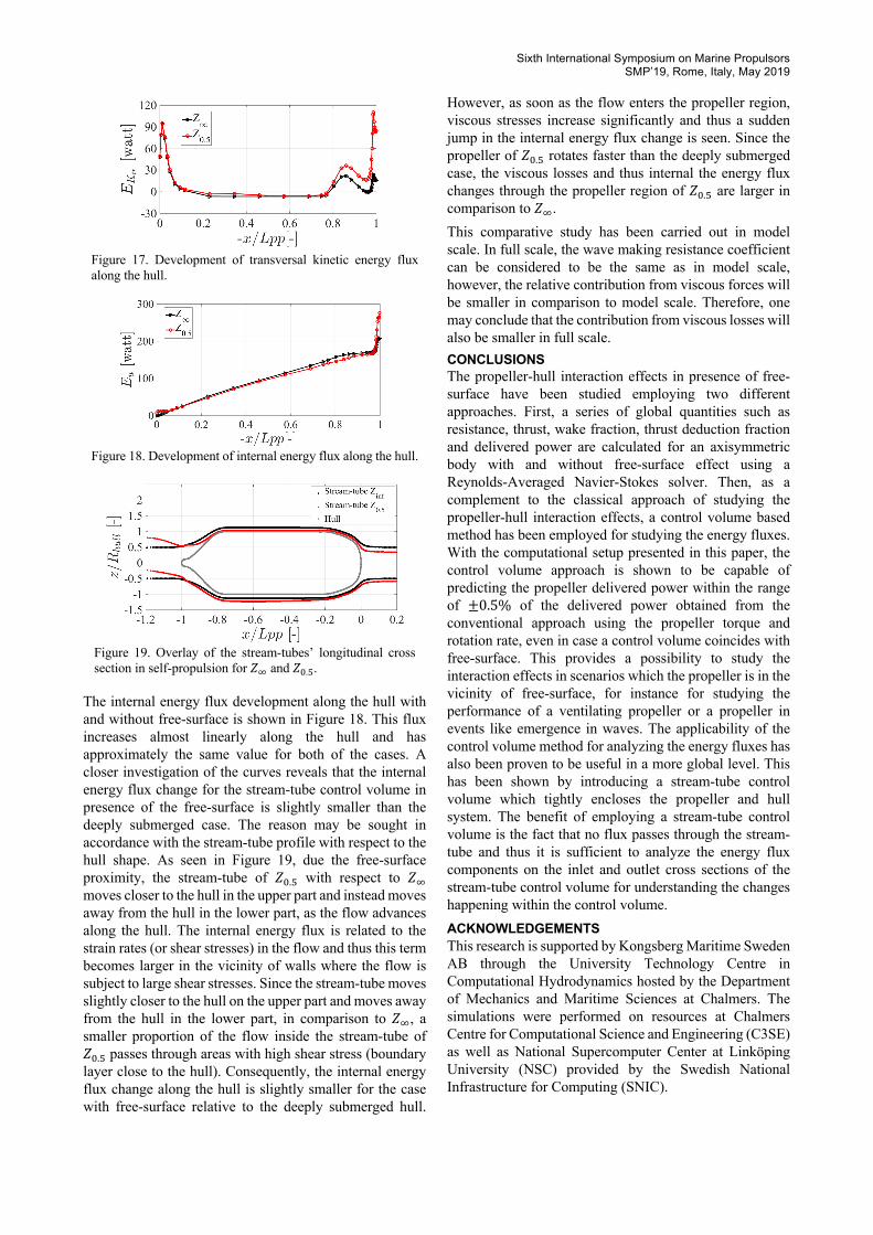
The effect of the hub vortex can be seen clearly in the transversal kinetic energy flux contour shown in Figure 12. Due to larger rotational velocity of the hub vortex for 𝑍L.N, transversal kinetic energy flux becomes more prominent than that of the 𝑍K. The higher propeller loading for this case also results in deflecting more flow into non-axial direction and thus transversal energy flux through the surface downstream the propeller increases rather significantly (about 24%, see Figure 9). The iso-surface of Q-criterion has been used in Figure 13 for visualization of the hub vortex as well as other vortical structures in the flow. Clearly it can be seen that these structures are more prominent for the propeller with higher load. Besides, a series of observations can be reported. In case of 𝑍K, the tip vortices generated from all the blades are almost identical, however the different tip vortexes show different behavior for 𝑍L.N. The reason is the uneven load distribution for the blades operating in an asymmetric wake. The blades operating in the starboard side are loaded more severely which can also be deduced from the large local axial kinetic energy flux contour shown in Figure 10.

𝐸𝐾𝑟𝑡 𝐸𝑢

Figure 12. Energy flux components downstream of the propeller.

Due to larger shear stresses for 𝑍L.N the dissipation of energy in form of internal energy increases relative to 𝑍K. From the contour plots given in Figure 12, it is seen that the stronger tip vortexes for the blades operating in the lower half of the hull wake result in larger internal energy flux in the same positions where the stronger tip vortices are observed.


Figure 13. Iso-surface of Q-criterion for 𝑍K (top) and 𝑍L.N (bottom).

The other interesting phenomenon is the hub vortex behaviour. As seen in Figure 13 the hub vortex for 𝑍L.N is inclined toward the free-surface, which is not the case when the free-surface effect is not present. The reason for the tilted hub vortex is rising flow in the aft which follows the free-surface profile. Similar to the bare hull’s stream-tube passing through the propeller disk (Figure 6) the stream-tube for self-propelled hull also rises behind the propeller and follow the free-surface (Figure 14). However, as shown in Figure 15, despite the slightly steeper stern wave in self-propulsion (see Figure 7) the stream-tube does not become as steep as the one for the bare hull. Due to the larger momentum of the flow after the propeller the flow tends to move straighter and deflect less in comparison to the bare hull case.

Figure 14. Limiting streamlines (black) and the stream-tubes passing through propeller disk (red) for bare hull 𝑍K (top) and 𝑍L.N (bottom). Free-surface profile is shown for 𝑍L.N along the hull in mid-section (blue).

Figure 15. Overlay of the stream-tubes’ longitudinal cross section for bare hull and self-propelled hull in presence of free-surface.

4.2.1 Stream-tube Control Volume Analysis To further understand the development of the energy loss terms along the hull, these terms have been studied employing the stream-tubes from self-propulsion (Figure 14). Per definition no flow passes through a stream-tube

and thus the energy flux change through the control volume only limits to the analysis of the fluxes through the cross section of stream-tube. In this study, the inlet of the stream-tube is assumed to be just ahead of the bow (𝑥/𝐿𝑝𝑝 =0.023). The cross section of this control surface with and without free-surface presence is shown in Figure 16. Because of the hull flow interaction with free-surface the shape of the stream-tube inlets control surface deviated from that of the deeply submerged hull. In general, this figure shows that the stream-tube tends to shift downward due to the proximity of the free-surface. The internal energy and transversal kinetic energy fluxes through several cross sections of the stream-tubes for𝑍K and 𝑍L.N have been extracted along the hull and their relative changes with respect to the stream-tubes’ inlet cross sections (Figure 16) are plotted in Figure 17 and Figure 18, respectively.

Figure 16. Cross section of the inlet area for stream-tube control volumes in self-propulsion.

Figure 17 shows the variation of transversal kinetic energy flux for stream-tube control volume with and without free-surface. The tangential velocity components are negligible along the hull, except in the region close to the propeller, and thus the main contribution to the transversal kinetic energy comes from the radial velocity components. Since the flow is deflected in the radial direction at the bow, the transversal kinetic energy flux increases locally. However, shortly after the fore-shoulders, the flow retains its axial direction and thus the transversal kinetic energy diminishes considerably. The relative development of transversal kinetic energy flux along the hull for 𝑍K and 𝑍L.N is very similar until the aft-shoulder (𝑥/𝐿𝑝𝑝 = 0.77), where they deviate from each other. Due to the reduced cross section of the hull in the stern region, the flow obtains an inward radial component which is the reason for the increased transversal kinetic energy flux in the region. Beside the overall trend which is similar for the case with and without free-surface, it is seen that the transversal kinetic energy flux becomes larger for 𝑍L.N relative to 𝑍K. The reason is the increased transversal (radial) velocity due to larger ingested flow into the propeller. The transversal kinetic energy flux increases abruptly when the flow reaches to the propeller (𝑥/𝐿𝑝𝑝 = 0.96). The reason for such an abrupt increase is the propeller induced swirl. Since the propeller of 𝑍L.N rotates about 37% faster relative to 𝑍K, it has a much higher transversal kinetic energy flux. Right after the propeller, this term starts to diminish quickly and eventually in far downstream reaches to zero.


Figure 17. Development of transversal kinetic energy flux along the hull.

Figure 18. Development of internal energy flux along the hull.

Figure 19. Overlay of the stream-tubes’ longitudinal cross section in self-propulsion for 𝑍K and 𝑍L.N.

The internal energy flux development along the hull with and without free-surface is shown in Figure 18. This flux increases almost linearly along the hull and has approximately the same value for both of the cases. A closer investigation of the curves reveals that the internal energy flux change for the stream-tube control volume in presence of the free-surface is slightly smaller than the deeply submerged case. The reason may be sought in accordance with the stream-tube profile with respect to the hull shape. As seen in Figure 19, due the free-surface proximity, the stream-tube of 𝑍L.N with respect to 𝑍K moves closer to the hull in the upper part and instead moves away from the hull in the lower part, as the flow advances along the hull. The internal energy flux is related to the strain rates (or shear stresses) in the flow and thus this term becomes larger in the vicinity of walls where the flow is subject to large shear stresses. Since the stream-tube moves slightly closer to the hull on the upper part and moves away from the hull in the lower part, in comparison to 𝑍K, a smaller proportion of the flow inside the stream-tube of 𝑍L.N passes through areas with high shear stress (boundary layer close to the hull). Consequently, the internal energy flux change along the hull is slightly smaller for the case with free-surface relative to the deeply submerged hull.

However, as soon as the flow enters the propeller region, viscous stresses increase significantly and thus a sudden jump in the internal energy flux change is seen. Since the propeller of 𝑍L.N rotates faster than the deeply submerged case, the viscous losses and thus internal the energy flux changes through the propeller region of 𝑍L.N are larger in comparison to 𝑍K. This comparative study has been carried out in model scale. In full scale, the wave making resistance coefficient can be considered to be the same as in model scale, however, the relative contribution from viscous forces will be smaller in comparison to model scale. Therefore, one may conclude that the contribution from viscous losses will also be smaller in full scale. CONCLUSIONS The propeller-hull interaction effects in presence of free-surface have been studied employing two different approaches. First, a series of global quantities such as resistance, thrust, wake fraction, thrust deduction fraction and delivered power are calculated for an axisymmetric body with and without free-surface effect using a Reynolds-Averaged Navier-Stokes solver. Then, as a complement to the classical approach of studying the propeller-hull interaction effects, a control volume based method has been employed for studying the energy fluxes. With the computational setup presented in this paper, the control volume approach is shown to be capable of predicting the propeller delivered power within the range of ±0.5% of the delivered power obtained from the conventional approach using the propeller torque and rotation rate, even in case a control volume coincides with free-surface. This provides a possibility to study the interaction effects in scenarios which the propeller is in the vicinity of free-surface, for instance for studying the performance of a ventilating propeller or a propeller in events like emergence in waves. The applicability of the control volume method for analyzing the energy fluxes has also been proven to be useful in a more global level. This has been shown by introducing a stream-tube control volume which tightly encloses the propeller and hull system. The benefit of employing a stream-tube control volume is the fact that no flux passes through the stream-tube and thus it is sufficient to analyze the energy flux components on the inlet and outlet cross sections of the stream-tube control volume for understanding the changes happening within the control volume. ACKNOWLEDGEMENTS This research is supported by Kongsberg Maritime Sweden AB through the University Technology Centre in Computational Hydrodynamics hosted by the Department of Mechanics and Maritime Sciences at Chalmers. The simulations were performed on resources at Chalmers Centre for Computational Science and Engineering (C3SE) as well as National Supercomputer Center at Linköping University (NSC) provided by the Swedish National Infrastructure for Computing (SNIC).


REFRENCES Andersson, J., Eslamdoost, A., Capitao Patrao, A.,

Hyensjö, M., & Bensow, R. E. (2018). Energy balance analysis of a propeller in open water. Ocean Engineering, 158. http://doi.org/10.1016/j.oceaneng.2018.03.067

Andersson, J., Eslamdoost, A., Vikström, M., & Bensow, R. E. (2018). Energy balance analysis of model-scale vessel with open and ducted propeller con fi guration. Ocean Engineering, 167(August), 369–379. http://doi.org/10.1016/j.oceaneng.2018.08.047

Andersson, J., Gustafsson, R., Eslamdoost, A., & Bensow, R. (2018). On the Selection of Optimal Propeller Diameter for a 120m Cargo Vessel. In The 15th Propeller and Shafting Symposium. Norfolk, Virginia, USA.

Bertram, V. (2012). Practical Ship Hydrodynamics (2nd ed.). Elsevier Ltd.

Dyne, G. (1995). The principles of propulsion optimization. In Trans. RINA 137. London, United.

Dyne, G., & Jonsson, L. . (1989). A Method for Analysing and Simulating Propulsion Systems. In International Symposium on Practical Design of Ships and Mobile Units (PRADS), 4th. Bulgarian Ship Hydrodynamics Centre, Varna, Bulgaria.

Dyne, G., & Lindell, P. (1994). Waterjet Testing in the SSPA towing Tank. In International Symposium if Waterjet Propulsion, RINA. London: The Royal Institute of Naval Architects.

Eslamdoost, A., Andersson, J., Bensow, R., Gustafsson, R., & Hyensjö, M. (2017). Analysis of Propeller-Hull Interaction Phenomena on a Self-Propelled Axisymmetric Body. In Fifth International Symposium on Marine Propulsors. Espoo, Finland.

Faltinsen, O. m. (2005). Hydrodynamics of High-Speed Marine Vehicles. Cambridge University Press. http://doi.org/https://doi.org/10.1017/CBO9780511546068

Haung, T., Liu, H. L., Groves, N., Forlini, T., Blanton, J., & Gowing, S. (1992). Measurements of Flows Over an Axisymmetric Body With Various Appendages in a Wind Tunnel: the DARPA Suboff Experimental Program. In 19th Symposium on Naval Hydrodynamics (pp. 321–346). Seoul, Korea.

Molland, A. F., Turnock, S. R., & Hudson, D. A. (2011). Ship Resistance and Propulsion. Cambridge University Press.

Moreno, M., Perez-Rojas, L., & Landweber, L. (1975). Effect of wake on wave resistance of a ship model. Iowa City, IOWA.

Muzaferija, S., & Perić, M. (1999). Computation of free surface flows using interface-tracking and interface- capturing methods. In Nonlinear Water Wave Interaction (pp. 59–100). Southampton: WIT Press.

Schuiling, B., & van Terwisga, T. (2016). Energy Analysis of a Propeller in Open Water Using a RANS Method. In 24th International HISWA Symposium on Yacht Design and Yacht Construction. Amsterdam, The Netherlands.

Schuiling, B., & van Terwisga, T. (2018). Energy Loss Analysis for a Propeller operating behind a Ship. In 32nd Symposium on Naval Hydrodynamics. Hamburg, Germany,.

Terwisga, T. (2013). On the working principles of Energy Saving Devices. In 3rd International Symposium on Marine Propulsors. Launceston, Australia.

Documents

Application of Control Volume Energy Balance for Analysing