Appendix: NetLogo Tutorial - Home - Springer978-3-319-29954-9/1.pdf · Appendix: NetLogo Tutorial 161. to procedureName do the necessary procedure commands here end Say we wantto

Appendix: NetLogo Tutorial

This appendix contains a quick introduction to programming in the NetLogo

system. A more detailed set of instructions is available at:

https://ccl.northwestern.edu/netlogo/docs/

General Things

Let us begin learning about NetLogo programming by trying some built-in

commands. First, select the Filemenu and then select New. Your text cursor shouldbe in a panel near the bottom called Command Center. The text cursor should be

flashing in a text area with the word observer next to it. NetLogo programming

commands are given to various types of agents that can respond to the commands.

The main two types of agents we are concerned with right now are the observer andturtles. To change the agent type you want to give commands to, you can select the

type by selecting it with the mouse. You can also use your tab key to move through

the agent types. Try both methods now.

Now click on the settings button near the top right of the screen. Notice that the

model world is a 2-dimensional grid of non-movable agents called patches. Theorigin (0, 0) is in the center by default with the x-axis going from �16 to 16 and the

y-axis is the same. Turtles are movable agents that can move around the world.

Click OK to save the world settings.

Built-In Commands, Turtles, and Variables

Try your first built-in command. Type the observer command show 2 + 2 in the

command center and press enter. You should see a response from the observer

agent in the command center text area showing the calculated answer 4. NetLogoalready knows about numbers and how to add them. Try other basic arithmetic.

Hint: the basic arithmetic operators are +, �, *,/.

Now try the command create-turtles 1. This asks the observer agent to create

one movable turtle with a random color and heading, default shape, and location.

Do you see a pointer near the center of the world? Change the agent type to turtles.

# Springer International Publishing Switzerland 2016

K. Brewer, C. Bareiss, Concise Guide to Computing Foundations,DOI 10.1007/978-3-319-29954-9

159

https://ccl.northwestern.edu/netlogo/docs/

Give your turtle the command set color red. Do you see a change in your turtle’s

color? Try changing the turtle to another color.

If you want to clear the world and start over, you can give the observer agent the

command clear-all. Try it now. Did your turtle disappear? Before continuing,

create 1 turtle in the world.

Change the agent type to turtles. You should only have one turtle in the world

right now, but these commands are sent to all turtles in the world. You’ll try more

turtles later. Each turtle has a set of variables with values specifically for that turtle.

You can see the variables and their values for your turtle with the command inspectturtle 0. You can also get this information by clicking on Tools menu and selecting

Turtle Monitor. Another way to monitor a turtle is to right click the mouse on a

turtle and select inspect turtle from the pop-up dialog.

Values of variables associated with agents can be changed using the set com-

mand. You already changed the color variable of your turtle for example with the

command set color red. You just give the agent the command (set) followed by the

variable you want to change (color) and the value you want to change it to (red).Since turtles are movable agents, they can change their world grid coordinates

(xcor, ycor). You can move the turtle to grid location (2, 2) with these two

commands set xcor 2 set ycor 2. There is also a shorter alternate command setxy2 2 that does the same thing. Try moving the turtle to location (2, 2). Did it work?

Try moving the turtle to other locations.

To save time typing in the command center, you can use the up and down arrow

keys to go back over command history and edit commands before pressing enter to

run the command. Use the arrow keys to go back to a previous command and

change it slightly before running it again. Did you get the results you expected in

the world?

The direZction a turtle is “heading” is represented by a compass heading as a

number of degrees from 0 to 359. Remember that 0¼ north, 90¼ east, 180¼ south,

270¼west. Note: this is not the same as the normal orientation used in geometry

and trigonometry which starts at 0 to the right and increases going counter-

clockwise. Change your turtle’s heading to east. Your turtle should now be heading

toward the right of the world, which is east. Try changing the turtle heading to other

directions. Think about what the result should look like before you run the com-

mand. Then run it and see if you get the result you expected.

You’ve already changed the turtle’s absolute world grid location and heading.

You can also change the turtle’s relative location and heading. Each turtle knows itsgrid location and heading. Giving a turtle the command forward 4 tells the turtle tomove straight ahead 4 patches. You can also change the heading from the current

heading with right 90. This makes a 90 degree or right turn relative to the current

heading. Try making some turns and moving around in the world to get a feel for

controlling the turtle.

Each turtle has a pen that can be raised or lowered to leave a mark where the

turtle has been. These turtle commands are pen-up and pen-down respectively. Try

putting the pen-down and making a square that is 10 patches by 10 patches in the

world grid. Carefully plan the steps the turtle must make to move along each side of

160 Appendix: NetLogo Tutorial

the square. Then try to give the sequence of commands to make the turtle complete

the square.

Repetition

Often you can shorten a procedure that repeats a sequence of commands. The

simplest repetition control structure in NetLogo is repeat which repeats a fixed

number of times on a sequence of commands. Change the color of your turtle and

then try this command repeat 4 [forward 10 right 90]. Forward 10 right 90 is a

sequence of commands which must be enclosed in brackets. This sequence of

2 commands is repeated 4 times. The computer must still run all 8 commands,

but it is shorter for you to give the command. It achieves the same result as writing

out all 8 commands as a single sequence.

Notice that after the turtle draws a 10 x 10 square, it is heading in the same

direction as it was before drawing the square. Give the right 5 command. Now use

the command editor to run the command that draws a square again. Repeat these

two commands several times and watch the pattern that is developing.

With the command editor, repeat a sequence of commands the number of times

you just calculated. The sequence of commands in brackets should include the

commands to draw a square followed by a command to turn right 5 degrees. Does it

look like you planned? If not, try to figure out why.

Selection

NetLogo has the command ifelse for selecting between 2 sequences of instructions

depending on some condition that is true or false. To see how it works, clear

everything and create one turtle. Now try this command for the turtle: ifelseheading mod 10< 5 [set color yellow] [set color green]. This command checks

the condition heading mod 10< 5. This divides the turtle’s current heading by

10 and checks to see if the remainder is less than 5. Since the remainder of dividing

any number by 10 must be between 0 and 9, headings that end between 0 and

4 degrees will be true and those that end between 5 and 9 will be false. When the

condition is true, the turtle color will be set to yellow. When it is false, the color will

be set to green. Did it work correctly? Change the heading using the set headingcommand. Then use the command editor to run the same ifelse command and see if

it does something different. It only does one of the set color commands when

it runs.

Procedures

A reusable set of instructions, a procedure, can be created in the Code tab. The basic

structure of a procedure is:

Appendix: NetLogo Tutorial 161

to procedureName

do the necessary procedure commands here

end

Say we want to have a turtle draw a square. The movement of a turtle in a square

would be repeat 4 [forward 10 right 90] and the turtle is right back where it started.Say we associate the name draw-square with this procedure:

to draw-square

pen-down

repeat 4 [forward 10 right 90]

pen-up

end

To use a procedure, just write the name. For the above turtle procedure to draw a

square, the code could be:

Clear-all

Create-turtles 1

ask turtles [ draw-square ]

Setup and Go

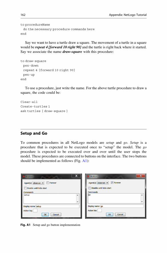
To common procedures in all NetLogo models are setup and go. Setup is a

procedure that is expected to be executed once to “setup” the model. The goprocedure is expected to be executed over and over until the user stops the

model. These procedures are connected to buttons on the interface. The two buttons

should be implemented as follows (Fig. A1):

Fig. A1 Setup and go button implementation

162 Appendix: NetLogo Tutorial

A Basic Model

A basic, simple model is therefore:

;; A simple 1st NetLogo program

to setup

clear-all

create-turtles 1

reset-ticks

end

to go

ask turtles [

draw-square

set heading heading + 10

]

end

to draw-square

pen-down

repeat 4 [forward 10 right 90]

pen-up

set color random 20

end

Appendix: NetLogo Tutorial 163

Appendix: LabQuest Tutorial

This appendix contains step-by-step instructions on how to use the LabQuest units.

A more detailed set of instructions is available from the manufacturer at:

http://www.vernier.com/files/manuals/labquest_quickstart_guide.pdf

Overview

The LabQuest instrumentation system consists of a LabQuest unit, sensors, and the

LabQuest software. The system has been designed for educational/classroom use,

so it has been made flexible and simple. The LabQuest units have a pressure

sensitive touch-screen interface that works best using the attached stylus.

Additional help and explanation of the system can be found at the

manufacturer’s website: http://www.vernier.com

Adding Sensors

Sensors are plug and play and either plug-in on the side or top of the LabQuest unit(depending on the sensor plug—the two kinds are similar, so if a sensor plug

doesn’t fit in the top, try the side. . .). Since the sensors are plug and play, nosetup or device management configurations are needed for the LabQuest to recog-

nize and start collecting data from a sensor. Sensors can be added or removed at any

time. Up to 6 different sensors can be attached at one time.

LabQuest Interface Overview

The software interface is a set of screens that provide control and display of

attached sensors. There are three main screens that can be accessed by pressing

the respective icons at the top of the display.



165

http://www.vernier.com/files/manuals/labquest_quickstart_guide.pdf

http://www.vernier.com/

Meter view

Graph view

166 Appendix: LabQuest Tutorial

Datatable view

The Meter View is where you can change the data collection settings for the

sensors, and can reset zero values and calibrate the sensors (for some sensors). The

Graph View is where you see your collected data, and where you can interact with a

graph of your data and perform simple analyses. This is also the view where you

will be able to export your data. The Datatable View shows your data in tabular

format. You can also export your data from this screen, if desired.

Changing Sensor and Data Collection Settings

From the Meter View screen, the Sensors menu will show all available actions for

your attached sensors.

Appendix: LabQuest Tutorial 167

1. Sensor Setup. . .—you will rarely need to setup a sensor as this is automatically

handled when you plug the sensor in. Use this only if you think your sensors are

not behaving properly (or just unplug and plug them back in).

2. Data Collection. . .—this is where you can change how data will be collected via

the sensor. Out of the many options for each sensor, you will likely just change

the frequency and length of time for your data collection. Note that there is a

maximum collection rate and maximum data values that can be collected, which

may limit your frequency/sample time choices.

3. Change Units—this will allow you to collect data in different (but appropriate)

units.

4. Calibrate—this will allow you to calibrate your sensor, if necessary. This is

often not needed.

5. Zero—this will allow you to set the zero value for your sensor.

6. Reverse—this will allow you to reverse the numeric response of the sensor.

Collecting Data

After sensors are plugged in, they immediately begin “sensing” and displaying

values on the Meter View screen. To collect a dataset, you need to press the collectbutton (that looks like it has a play symbol, go figure). After a brief initialization

period, the LabQuest will begin collecting and displaying data in the Graph View. If

you want to stop data collection before the end of the Sample Time, you can press

the collect button again. Data collection automatically stops at the end of the

Sample Time.


Analyzing Data

After you collect data, you can use the LabQuest unit to perform some simple

analyses. One of the most common techniques is to obtain simple statistics about

your data. From the Graph View screen, select Statistics from the Analyzemenu and

then select (via check box) the data you wish to analyze (in the following example,

it is Sound Pressure).


To the right side of the graph, the light blue box will display basic statistics on

your data. If you click that box, it will bring up a full screen view.

Getting Data to Excel

Once you have collected your data, you can export it to your computer to use in

Excel (or other program). You will need a USB thumb drive. Follow the following

steps:

1. Plug in your USB thumb drive in the USB port at the top of the LabQuest.

2. From the Graph View or Datatable View screen, select Export. . . from the Filemenu.


3. Tap on the USB thumb drive icon.

4. Tap the Name: field and enter the filename for your data. Use.txt as your fileextension.

5. Tap OK and your data will be saved.

6. When finished (your USB thumb drive light stops flashing), un-plug your

thumb drive.


7. Plug your thumb drive into your USB port on your computer.

8. Open your file in your computer’s file system viewer (Windows Explorer on

Windows; Finder on MacOSX). Move your file to the working directory of

your choosing.

9. Open Excel.

10. Select Open from the File tab/menu. Change the file type to All files (*.*).11. Open your data file.

12. In the Text Import Wizard—Step 1 of 3, choose Delimited Row 1 and UTF-8 (these may be the default selection). Click Next.

13. In the Text Import Wizard—Step 2 of 3, choose Tab (this may be the default

selection). Click Next.14. In the Text Import Wizard—Step 3 of 3, leave all the default settings and click

Finish.15. You are now viewing your data in Excel, column format. Each data point is a

separate row.

Reference

Software from Vernier Software & Technology and LabQuest App


Appendix: GIS Tutorial

This appendix contains step-by-step instructions on how to use the gvSIG version

1.11 GIS software. More recent versions of the software may behave differently.

Join by Attribute

1. Start gvSIG.

2. Click on the View icon.

3. Click on the New button. You should now see:



173

4. Double-click the Untitled �0 item in the list. This will bring up the following

window:

5. Click the Add Layer icon (or find the Add Layer menu item under the

View menu).

6. Click the Add button and from the standard windows file dialog, select (use the

open button in the dialog) ILCounties.shp file.7. Click the Add button again and select the ILCities.shp file.8. Click OK. The counties and cities in Illinois should now be displayed in a map

view. Resize the window to your liking. Double click the colored rectangle just

below the counties.shp text in the legend to change the appearance of the

counties, if desired. (You can do the same for the cities.). Your map/window

should look something like:

174 Appendix: GIS Tutorial

9. Explore the attributes for both the cities and counties. Click on ILCities.shp in

the legend (the typeface will become bold, indicating it is the active layer) and

then click on the Show attribute table of active layer icon in the toolbar. Resizethe resulting window as required.

Appendix: GIS Tutorial 175

10. At the bottom of the table view, the total number of records are given for that

layer. The above image shows that there are 180 cities in the ILcities.shp layer.

(How many counties are there in the ILCounties.shp layer?)

11. Before you join the county data to the city data using attributes, you need to

know what the key fields are named in each layer. After you determine that, you

can proceed.

12. To join based on attributes, with the attribute tables for both the ILCities.shp

layer and ILCounties.shp layer visible, click the Join. . . icon.13. The first entries are for the destination table.


14. After clicking Next, the second entries are for the source table.

15. Click Finish and your ILCities.shp attribute table now has the appropriate

county data fields added for each city record.

Spatial Join

1. Start gvSIG.

2. Click on the View icon.

3. Click on the New button.

4. Double-click the Untitled �0 item in the list.

5. Click the Add Layer icon (or find the Add Layer menu item under the

View menu).

6. Click the Add button and from the standard windows file dialog, select (use the

open button in the dialog) USACounties.shp file.


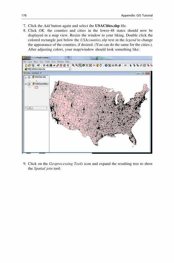
7. Click the Add button again and select the USACities.shp file.

8. Click OK. the counties and cities in the lower-48 states should now be

displayed in a map view. Resize the window to your liking. Double click the

colored rectangle just below the USAcounties.shp text in the legend to change

the appearance of the counties, if desired. (You can do the same for the cities.).

After adjusting colors, your map/window should look something like:

9. Click on the Geoprocessing Tools icon and expand the resulting tree to show

the Spatial join tool:


10. Click the Spatial join tool to bring up its description. Click the Open tool. . .button to open the tool’s dialog box. The Input layer is the destination layer,

and the overlay layer is the source layer. Choose a file name and location to

save your joined layer.


11. Open the attribute table for the joined layer and notice that the right half of the

attribute columns are all county data.


Definitions

(A)

• Abstraction—general concept created from specific examples.

• Active site—pocket or cleft in a protein which is surrounded by amino acid side

chains that help to bind the substrate and other side chains that play a role in the

catalytic process.

• Accuracy—closeness of instrument-reported values to actual measurement

values.

• Agent-based modeling—representation of a system–as a collection of autono-

mous decision-making agents that individually assess their situations and make

decisions based on a set of rules.

• Algorithm—set of instructions that solves a particular problem.

• Amino acid—group of organic compounds containing both carboxyl and amino

groups. There are 20 different kinds of amino acid molecules, each of which are

commonly represented by a unique capital letter.

• Anisotropic—a property or parameter that varies depending on the direction of

measurement

• ArcGIS—industry-standard GIS program sold by ESRI.

• Array—data structure with homogeneous data; each item can be directly

addressed by a unique id that is sequential.

• ASCII—American Standard Code for Information Interchange. A standard for

mapping single characters to an unique 7 bit number

• Attribute—information about a spatial object; multiple attributes are stored in

fields in attribute tables.

(B)

• Big-Oh classes—common simplified functions that are upper bounds for actual

time complexity functions in which algorithms are classified as “On the Order of”

a group.

• Bimolecular—type of reaction initiated when two molecules collide.

• Binary—Base 2 number system whose only allowed digits are 0 and 1

• Binary tree—tree in which each node may have, at most, two children (a left and

a right child).

• Bit—a single digit in binary



181

• Boundary conditions—the definition of how the unknown value is defined at the

boundaries of the domain. There are three main types of boundaries (Dirichlet,

Neumann, and Cauchy).

• Byte—8 bits

(C)

• Calibration—the alteration of numerical model parameters to minimize error of

numerical model results to actual (known) data.

• Cardinality—relationship between two data sets based on some commonality. In

ArcGIS, x -to- y cardinality refers to the destination -to- source data.

(Possibilities are: one -to- one, one -to- many, many -to- one, and many -to-

many.)• Cauchy Boundary Conditions—flux across the boundary is dependent on the

unknown variable value.

• Chain—one portion of a protein

• Compression—process of taking a file and making it smaller so that the original

(or close approximation of the original) can be restored.

• Computational Science—field of study concerned with using computers to run

numerical calculations of mathematical models to analyze and solve scientific

problems.

• Concentration—amount of solution per unit volume. In Chemistry, concentra-

tion is often measured as moles of solute per liter of solution.

• Constraints—equations or limits on parameters due to physical or other reasons.

• Convergence—the process of reducing the error to a minimum during an itera-

tive process.

• Curve fitting—the process of finding the best curve to fit a set of data points

(D)

• Database—collection of self-describing integrated records.

• Data set—group of related data.

• Data structure—system to organize data in a particular way.

• DBMS—Database Management System, software that maintains a database.

• Decimal—Base 10 number system with digits from 0 to 9

• Design—the process of deciding how an algorithm or simulation should work

before coding it

• Dirichlet Boundary Conditions—the unknown variable is known and defined at

the boundary.

• Discritization—is process of creating a finite element or finite difference grid in

a domain.

• Domain—is the area (or volume) of interest that is constrained by boundary

conditions.

• Dominant term—fastest growing term in a time complexity function and is used

to determine the Big-Oh class.

182 Definitions

• Drift—tendency for reported instrument values to slowly change over time

(when the actual measurement isn’t changing), commonly due to electronics

issues in the instrument and sensor.

• Dynamic systems modeling—representation of a system using feedback loops

and stacks and flows.

(E)

• Equilibrium—state in which a reaction appears not to progress any further.

Concentrations of the reactants and products reach a dynamic state in which

the forward and reverse reactions are equal.

• Expectation value—average value of an observable property of a system

measured once on many identically prepared experimental models.

(F)

• Feature—spatial object that uses either the raster or vector model.

• Feature Classes—grouping of like features in a GIS system. (Also called DataSets.)

• Finite difference—a numerical technique to solve partial differential equations

in a domain using algebraic equations and a grid.

• Finite element—a numerical technique to solve partial differential equations in a

domain using a series of interpolation functions and a triangular grid.

• Floating point—integer followed by a decimal point and an integer.

(G)

• Genetic algorithm—optimization technique/method based on an analogy of

genetics and evolutionary theory/natural selection.

• Geodatabase—object-oriented model for storing spatial information used by

ArcGIS. Constructed on the architecture of standard relational database systems

(for small, personal geodatabases, ArcGIS uses Microsoft Access). Contains

feature classes (i.e., spatial objects of a similar type), tables, relationships,

network information. A “robust” implementation, topology (i.e., relationship

rules between spatial objects), network (i.e., connectedness), and behavior and

validation rules.

• GIS—Geographic Information System,

• Graph—data structure with nodes that are connected with edges.

(H)

• Heme—prosthetic group that consists of an iron atom in the center of a large,

heterocyclic organic ring called a porphyrin.

• Heterogeneous—a property or parameter that varies in space

• Heuristic search—A search method to find a satisfactory solution using

shortcuts or preexisting experience. Examples include using a rule-of-thumb or

educated guess to shorten the search time or minimize required resources

(e.g. storage). The search is not guaranteed to be complete.

• Hexidecimal—Base 16 number system with digits from 0–9 and a-f

• Homogeneous—a property or parameter that does not vary in space

Definitions 183

(I)

• Integer—any whole number including 0 and negative numbers.

• Isotropic—a property or parameter that does not vary depending on the direction

of measurement

• Iteration—the repetition of a solution algorithm/method to arrive at a converged

solution.

(J)

• Join—combination of two tables based on common attributes or spatial

relationship.

(K)

• Key (field)—common field that is used when combining tables.

• Kinetics—study of motion with respect to time. In Chemistry, the term refers to

the study of the progress of reactions over time and the mechanisms through

which reactions proceed.

(L)

• Ligand—ion or molecule attached to a metal atom by bonding in which both

electrons are supplied by one atom.

• Linked list—data structure with homogeneous data in which each item knows

where the next item is.

• Lossless compression—compression method that guarantees the exact restora-

tion of the original.

• Lossy compression—compression method that does not guarantee the exact

restoration of the original.

(M)

• Markup language—language that uses tags to describe its contents.

• Model—mathematical representation of some scientific phenomenon or system.

(N)

• Neumann Boundary Condition—flux across the boundary is known and defined.

(O)

• Objective function—mathematical function designed to represent a system.

• Optimization—process of finding the best solution.

(P)

• Parameter—independent variable

• Particle in a box—type of mathematical problem used as a simple model for

quantum mechanics problems.

184 Definitions

• Performance—inverse proportion of the time required to run a procedure on a

computer system. shorter run time means higher performance.

• Pixel—single addressable dot on a graphical computer display.

• Polypeptides—short chains (50 or fewer) of amino acids linked by peptide

bonds.

• Potential energy well—region in which limitations are set on the particle of a

box problem. The box is made finite with infinite potential energy “walls.”

• Precision—number of significant digits for an attribute measurement.

• Procedural abstraction—association of a procedure with a name. The procedure

can then be run by using its name.

• Procedure—algorithm written in a computer programming language that can be

run on a computer. (Also called a program or subprogram.)

• Projection—coordinate transformation from three-dimensions on a “globe” to a

two-dimensional representation on “paper” in which distortion results in one or

more properties: area, distance, shape, and/or direction.

• Prosthetic group—small molecule that is either noncovalently or covalently

bonded to a protein to fulfill a special function.

• Protein—group of organic compounds composed of one or more chains of

amino acids and forms an essential part of all living organisms. Typical proteins

consist of 50–1000 amino acids. Humans make at least 50,000 different proteins,

and a typical cell may contain 7000–10,000 different proteins.

(Q)

• Quantum mechanics—mathematical system used to model the structure and

behavior of atoms and molecules. Predicts that there are discrete energies

allowed for subatomic particles.

• Query—extraction of information from a database or table based on defined

attribute criteria or spatial criteria.

• Query sequence—The sequence a researcher has and wants to match to other

known sequences in a database, to determine if the sequence of interest (the

query sequence) is similar to an already-described protein or gene

(R)

• Raster graphics—representation of images as rectangular grids of pixels. (Also

called a bitmap.)• Raster model—representation of spatial data as a grid of cells (pixels). Each cell

has one numeric value.

• Rates—speed (or change per unit time). In Chemistry, the rate of a reaction is

usually measured as a change in concentration of a reactant or product per unit

time elapsed.

• Reaction—a process that changes a chemical substance (or substances) into

another (others).

• Regression—a mathematical process of comparing and systematically reducing

the differences between an estimated value and a known value.

• Relation—table in a database.

Definitions 185

• Reliability—ability to rely or depend on results from a simulation to faithfully

represent a real world phenomenon or system. Problems include (1) incorrect

model, (2) incorrect model representation, and (3) computational errors.

• Resolution—rectangular grid dimensions of pixels on a computer display

(e.g. 1280� 1024); or the finest, discernible difference in reported measured

values, due to electronics and physical limitations of the sensor technology

(S)

• Sampling frequency—number of measurements that will be reported during a

given amount of time (e.g. 5 samples per second). Related to sampling interval.• Sampling interval—amount of time between reported sampling values. Related

to sampling frequency.• Sampling length—amount of measurement time.

• Self-defining—information that contains a description of its structure within

itself.

• Sensitivity analysis—an analysis performed on a numerical model to assess

which parameters the model results are most sensitive to changes in.

• Sequence homology/percent identity—The similarity of two gene or protein

sequences (often expressed as % that is the same or % identity)

• Simulated annealing—optimization technique/method based on an analogy of

how metals that are slowly cooled end up with a better (lower energy, more

stable) crystal state.

• Simulation—computer model of the behavior of a real world phenomenon or

system.

• Splines—a set of cubic equations used to fit a fix number of points exactly

• Solvent—portion of a mixture that is in greater amount. A compound of interest

is often dissolved in a solvent.

• SQL—Structured Query Language. Format used for selection from databases

based on attribute data of the SELECT FROM WHERE form.

• Steady-state—a system that does not change with time.

• Substitution matrix—A matrix of scores to compare the probability of substitu-

tion of one amino acid for a different amino in differing protein sequences,

incorporating empirical data from changes in similar proteins. (i.e.—What is the

likelihood that the amino acid difference is due to evolutionary change in the

genetic sequences)

• Substrate—molecule upon which a protein acts.

• Sum of squares—the squaring of each number and summing of the resulting set

of numbers

(T)

• Table—two-dimensional collection of information organized by fields

(columns) and records (rows), in which attributes about spatial features are

stored.

• Target sequence—The sequence from a database that matches (with some

predefined level of % identity) the query sequence

186 Definitions

• Time complexity function—mathematical function that gives the time for a

procedure to run given the input size of the problem.

• Transient—a system that does change with time.

• Tree—graph in which each node (except the root) can have only one parent but

multiple children. The root has no parents.

• Trial-and-error—a process of trying solutions until the best one (least acceptable

error) is found.

(U)

• Uncertainty analysis—an analysis performed with a numerical model to assess

the uncertainty of model predictions resulting from the uncertainty of model

parameters.

• Unimolecular— type of reaction initiated when one molecule undergoes a

change.

(V)

• Validation—subjective analysis to determine if the simulation model correctly

describes the real world phenomenon or system.

• Vector graphics—representation of images as collections of mathematical

equations for lines (i.e. vectors). Often a more compact representation that

allows faithful image scaling.

• Vector model—representation of spatial objects as points, lines (polylines), or

polygons using a series of x y locations.

• Verification—objective analysis to determine if the computer simulation

correctly implements the model.

• Visualization—act of creating images, diagrams, or animations to improve

communication of results from a simulation model.

(W)

• Wave function—amplitude of a wave. In quantum mechanics, it acts as the

“path” that an electron moves around the nucleus of an atom.

• Word—the number of bits used by a computer for its standard size, typically

32 or 64 bits.

Definitions 187

Index

AAbstraction, 22–38, 45–56, 101

Accuracy, 25, 28–31, 39, 41, 42

Agent-based modeling, 9

Agents, 10, 19, 47, 50, 52, 53, 102

Algorithms, 5–7, 45–56, 69, 98–107,

111, 120, 122–126, 132–136,

139–149, 156, 157

American Standard Code Information

Interchange (ASCII), 30, 31

Amino acids, 120–122

Analytic solution, 60–62

Ancestors, 35, 36

Applications, 6, 98, 110

ArcGIS, 151

Arrays, 34, 36, 111

Attributes, 109, 152–156

BBase, 22–26, 105

Big-Oh classes, 105–107

Binary, 22, 24–26

Binary tree, 35, 38

Bits, 24–27, 30, 34, 71, 92, 111

Boundary conditions, 84, 85, 87, 92, 94

Byte, 25, 28, 30–31

CCalibration, 94

Cardinality, 154, 155

Characters, 22, 24, 30, 31

Command Center, 2, 102

Complexity, 97, 139

Compression, 109–118, 126

Computational science, 2–7, 9, 55, 98

Computations, 6, 7, 62, 86, 115

Concentration, 10–13, 15, 16

Constraints, 74–77, 79, 80, 85, 136, 138, 139,

145, 146, 148

Control structures, 46–48, 50

Convergence, 93

Curve fitting, 59, 129–135

DData abstraction, 52

Database management system (DBMS), 113,

114, 118

Databases, 42, 109–118, 120, 124, 125, 156,

157

Data set, 120, 152–156

Data structure, 36, 37, 110, 112

Data warehouse, 115–117

Decimal, 24–26

Descendants, 35

Design, 6, 43, 46, 65–70, 74, 76, 78, 80, 138

Destination, 154, 155

Directed weighted graph, 36

Domain, 6, 84, 86, 87, 91, 94, 140, 143

Dominant term, 106, 107

Drift, 39

Dynamic systems modeling, 9, 10

EEnqueue, 37

Equation solution, 59–60, 84

Equilibrium, 10, 11, 13, 14, 18

Errors, 5, 6, 19, 26–29, 44, 62, 71, 76, 81, 95,

101, 126, 129–136, 148, 156

Ethics, 7

Evolutionary method, 76

Expectation value, 125

Exponent, 25, 76, 131

EXtensible Markup Language (XML),

109–118



189

FFeatures, 13, 111

Feature Classes, 151

Field, 27, 69, 74, 116, 117, 152, 154,

156, 157

Finite difference (FD), 86–89, 92

Finite element (FE), 86

First-order reaction, 10, 15–19

Floating point, 22, 25–27, 29, 31, 44, 62, 81,

95, 125, 134, 148, 156

GGene sequence, 142

Genetic algorithm, 142–145

Geodatabase, 151

Giga, 24

Go, 2, 11–13, 48, 50, 52–55Goal seek tool, 69, 72

Graph, 10, 13, 16–18, 34, 36–37, 40, 41, 44, 55,

106, 112, 130, 131

GRG nonlinear method, 76

HHead, 37, 85–87, 89, 91–93

Heterogeneous, 31, 91, 148, 156

Heuristic search, 119

Homogeneous, 31, 35–38, 85, 86, 91

IInspection, 60–62, 85, 86

Integers, 22–29, 31, 34, 44, 62, 80, 81, 95, 104,

105, 125, 131, 134, 148, 156

Integration, 16

Isotropic, 85, 86, 91

Iteration, 55, 62, 89, 90, 93, 94

Iterative calculation, 90–91

JJava, 27, 29

Join/joining, 114–116, 118, 152–156

KKey (field), 152, 154, 156

Kilo, 24

Kinetics, 9–19

LLaplacian, 83, 86

Leaf, 35, 52–55

Linear, 10, 15, 39, 60, 61, 76, 92, 130–133,

136, 138, 145, 146, 148

Linear programming, 139, 145–146, 148

Linked list, 33, 34, 37

Lossless compression, 110, 111, 126

Lossy compression, 110, 111, 126

MMantissa, 25, 27

Markup language, 109

Mathematical model, 2, 5–7, 10, 53, 59, 84

MatLab, 93

Mega, 24, 125

Merge sort, 103–105

Model, 2, 9, 34, 48, 59, 84, 98, 112, 129, 140, 152

Mutation, 143, 144

NNetLogo, 2–7, 9, 11–15, 45–48, 51, 52, 55, 97,

102–104, 140, 141, 143, 144

Neumann boundary condition, 85

Non-linear, 85, 138

Numerical solution, 60–62

OObjective function, 136, 138, 139, 145–148

Optimization, 74, 135–149

Order of operation, 28–29

PParameters, 55, 67, 68, 70–74, 79, 80, 84, 91,

94, 133, 136–139, 142, 144–146

Parent, 35, 36, 142

Performance, 97, 139

Peta, 24

Pixels, 110, 152

Pop, 37

Precision, 28, 29, 39–42

Probe, 40, 42

Procedural abstraction, 48, 52

Procedure, 5, 6, 40, 43, 45–56, 97

Products, 10, 13, 16, 113–115, 117, 156

Projection, 151

190 Index

Proteins, 120–125

Push, 2, 37, 50, 53, 55

QQuery, 114, 124, 125

Query sequence, 120, 121, 123–125

Queue, 37–38, 112

RRaster graphics, 1

Raster model, 152

Rate constants, 11, 13

Rates, 10–12, 15–18, 69, 85, 101, 103, 105,

142, 145

Rational numbers, 25, 26, 29

Reactants, 10, 11, 13, 15, 16

Reaction, 9–19, 31, 41, 42

Real numbers, 80, 136

Record, 2, 22, 31, 40, 55, 59, 112, 120, 152,

154, 155

Regression, 132–133

Relations, 112, 113

Reliability, 13, 15

Repeating decimal, 26

Repetition, 46–48, 50

Resolution, 34, 43, 110

Reversible reaction, 11, 18–19

RK4, 16

Root, 35, 36, 60, 61, 76, 136

SSafety factor (factor of safety), 67, 71, 73, 79,

142, 145

Sampling frequency, 39, 43

Sampling interval, 39

Sampling length, 43

Selection, 46–48, 50, 69, 72, 142

Self-defining, 109–118

Sensitivity analysis, 94

Sequence, 46–51, 120, 121, 123–125, 142

Setup, 2, 11–13, 43, 44, 48–51, 53, 55, 104,137–139

Significant figures, 40, 41

Simplex LP, 76

Simplex Method, 139, 146–148

Simulated annealing, 139–142

Simulations, 2, 4, 6, 7, 11, 13, 15–17, 19, 49,

53, 55, 80, 81, 95, 98–99, 111, 140, 142,

143, 145, 148

Sliders, 2, 11–13, 49, 50, 55, 102, 131

Solver tool, 70, 74, 75, 77–80, 133

Sort, 13, 61, 84, 103–105, 115, 117, 120

Source, 5, 6, 19, 44, 62, 81, 95, 104, 126, 134,

148, 154–156

Spline, 61, 134

Stack, 37–38, 42, 112

Steady-state, 85, 86

Stress, 66–68, 70–72, 74, 75, 80

Structured Query Language (SQL), 116, 117

Substitution matrix, 121, 123

Sum of squares, 131, 133

TTable, 30, 32, 46, 67, 79, 112–118, 122, 147,

152–155, 157

Tableau, 147

Tera, 24

Three-d?, 4

Time complexity functions, 103, 105–107

Transient, 84, 85

Trees, 35–37, 112, 124

Trial, 68, 69, 73

Trial-and-error, 68–70, 73, 74, 132

Turtle, 47–53, 140, 143

UUncertainty analysis, 94

UniCode, 30, 31

VValidation, 110

Variables, 2, 12, 13, 51, 52, 54, 55, 60,

74–76, 84, 133, 136–138, 140, 143,

146, 147

Vector graphics, 32

Vector model, 152

Vensim, 10, 15, 16, 19

Verification, 1

Visualization, 4, 7, 9–19, 37, 131, 140, 143

WWord, 25, 30, 53, 89, 98, 123–125, 154

YYoung’s Modulus (Modulus

of Elasticity), 79

Index 191

Documents

Appendix: NetLogo Tutorial - Home - Springer978-3-319-29954-9/1.pdf · Appendix: NetLogo Tutorial 161. to procedureName do the necessary procedure commands here end Say we wantto