NetLogo-Mathematica LinkTutorials and Examples

This document will show how to use the NetLogo-Mathematica add-on to application interface. The notebook has examples that make useof sample models included with NetLogo. Click the right-most bracket of each cell to collapse a section.

Warning: It is important that you run install the link and execute the code in Starting NetLogo before continu-ing with the tutorial. You may skip around sections, but within each section, you must start from the top andexecute each consecutive command. Sections will not work properly if you do not follow the instructions step-by-step.

Installing the NetLogo-Mathematica LinkTo install the NetLogo-Mathematica link, go to the menu bar in Mathematica, click on File and select Install... In the Install MathematicaItem dialog, select Package for Type of item to install, click Source, and select From file... In the file browser, go to the location of yourNetLogo installation, click on the Mathematica Link subfolder, and select NetLogo.m. For Install Name, enter NetLogo. You can eitherinstall the NetLogo link in your user base directory or in the system-wide directory. If the NetLogo link is installed in the user basedirectory, other users on the system must also go through the NetLogo-Mathematica link installation process to use it. This option mightbe preferable if you do not have permission to modify files outside of your home directory. Otherwise, you can install NetLogo-Mathemat-ica link in the system-wide Mathematica base directory.

Starting NetLogoOnce installed, the NetLogo package can be loaded at any time with the following command:

In[21]:= << NetLogo`

To start NetLogo simply type the following command, and use the file browser to locate the NetLogo parent directory, typically located in"/Applications/NetLogo 4.0" or "C:\Program Files\NetLogo 4.0", on Macintosh and Windows systems, respectively.

In[22]:= NLStart@D

The NetLogo-Mathematica Link will store this path in $NLHome

In[23]:= $NLHome

Out[23]= êUsersêebakshyênetlogoê

One can also manually specify the $NLHome directory by hard coding in your NetLogo installation directory. This is preferable in manyreal-world scenarios when one uses the NetLogo-Mathematica Link often.

$NLHome = "êApplicationsêNetLogo 4.0ê";$NLHome = "C:\\Program Files\\NetLogo 4.0";

Once again, to start NetLogo using the default path (now specified by $NLHome) enter

In[24]:= NLStart@D

An Overview of the NetLogo-Mathematica Link using Fireü Loading a NetLogo model

Use NLLoadModel[] to load the Fire example from the models library.

In[25]:= NLLoadModel@ToFileName@8$NLHome, "models", "Sample Models", "Earth Science"<, "Fire.nlogo"DD;

ü Executing NetLogo commands

The NLCommand[] function lets you execute any NetLogo command as if you were typing from the command center.

In[26]:= NLCommand@"setup"D;

In[27]:= NLCommand@"set density 25"D;

The function NLCommand[] automatically splices expression into NetLogo strings, making it easy to pass sequences of strings, numbers,lists, and colors into NetLogo without having to manually convert data types and join strings.

In[28]:= NLCommand@"set density", 50D;

Splicing can be very useful for setting NetLogo sliders using Mathematica variables

In[29]:= d = 65;NLCommand@"set density", dD;

It is also possible to specify several command sequences using a single NLCommand[]

In[31]:= NLCommand@"set density", d - 10, "show density", "setup"D;

ü Repeatedly executing NetLogo commands

This loop calls NLCommand[] 10 times.

In[32]:= Do@NLCommand@"go"D, 810<D;

The command NLDoCommand[] is an easier and efficient way to execute a command repeatedly.

In[33]:= NLDoCommand@"go", 10D;

ü Reporting data from NetLogo

You can retrieve data from NetLogo using NLReport[]

In[34]:= NLReport@"count turtles"DOut[34]= 348.

ü Repeat reports n times

One of the simplest uses of the NetLogo-Mathematica link is to repeat a command and report information after each successive command.

A way carry out these kinds of repetitive tasks is to use NLCommand[] and NLReport[] in combination with Table[].

In[35]:= Table@NLCommand@"go"D; NLReport@"Hburned-trees ê initial-treesL * 100"D, 820<DOut[35]= 82.80936, 2.8588, 2.91115, 2.97223, 3.0333, 3.10019, 3.1758, 3.23688, 3.30958, 3.3852,

3.46081, 3.5277, 3.60622, 3.68765, 3.74291, 3.80398, 3.85052, 3.90286, 3.9523, 4.00756<

Tasks like these can be more easily and efficiently executed with NLDoReport[], which will successively execute a command andreturn a reporter n times.

In[36]:= NLDoReport@"go", "Hburned-trees ê initial-treesL * 100", 20DOut[36]= 84.04828, 4.07736, 4.10644, 4.13843, 4.17042, 4.21114, 4.26058, 4.3042, 4.34492, 4.39145,

4.44671, 4.49905, 4.54849, 4.59503, 4.65319, 4.691, 4.73753, 4.76952, 4.7986, 4.82478<

ü Repeat reports until a condition is met

NLDoReportWhile[] is similar to NLDoReport[], but rather than executing n times, it executes until a condition is [not]met.

The following executes "go" and reports back the % of trees burned until there are no turtles (embers) left.

The following executes "go" and reports back the % of trees burned until there are no turtles (embers) left.

In[37]:= NLCommand@"Setup", "set density", 55D;NLDoReportWhile@"go", "Hburned-trees ê initial-treesL * 100", "any? turtles"D

Out[38]= 80.370724, 0.585049, 0.825441, 1.03108, 1.20485, 1.37284, 1.54082, 1.70591, 1.84493, 1.96078,2.06505, 2.16642, 2.262, 2.35178, 2.43577, 2.52846, 2.62983, 2.7312, 2.82967, 2.93104,3.02372, 3.1193, 3.22646, 3.34521, 3.43789, 3.52188, 3.59429, 3.65221, 3.73041, 3.78544,3.82599, 3.86654, 3.91578, 3.9766, 4.03742, 4.08666, 4.1272, 4.16775, 4.2083, 4.25175,4.29229, 4.32415, 4.35022, 4.3647, 4.37629, 4.38497, 4.39946, 4.41104, 4.41104, 4.41104,4.41104, 4.41104, 4.41104, 4.41104, 4.41104, 4.41104, 4.41104, 4.41104, 4.41104, 4.41104<

Ë Defining a simple experiment

An interesting phenomena in the Forest Fire model is the abrupt change that occurs in size of forest fires as the density increases. In thisexample, we will write a short function which sets up the model and returns a list of the percentage of trees burned at each time step, untilall embers have burned out.

In[39]:= FireTimeSeries@density_D := Module@8<,NLCommand@"set density ", density, "setup"D ;NLDoReportWhile@"go", "Hburned-trees ê initial-treesL * 100", "any? turtles"D

D;Generate a list of densities to run the model with, ranging from 50 to 70 in increments of 2

In[40]:= densities = Table@density, 8density, 50, 70, 2<DOut[40]= 850, 52, 54, 56, 58, 60, 62, 64, 66, 68, 70<

Carry out the FireTimeSeries[] function with each density

In[41]:= NLCommand@"no-display"D;fireData = Map@FireTimeSeries, densitiesD;

Ë Plot time dynamics of each run

Now that we have recorded the time dynamics of each configuration, let's take a look at how the fire spreads in first configuration (density= 70)

In[43]:= ListPlot@First@fireDataD,AxesLabel Ø 8"Time", "% Burned"<, PlotLabel Ø "Burn time series at density = 50"

D

Out[43]=

20 40 60 80Time

1.0

1.5

2.0

2.5

3.0

3.5

% BurnedBurn time series at density = 50

With a little bit more work, we can plot all the time series data simultaneously.

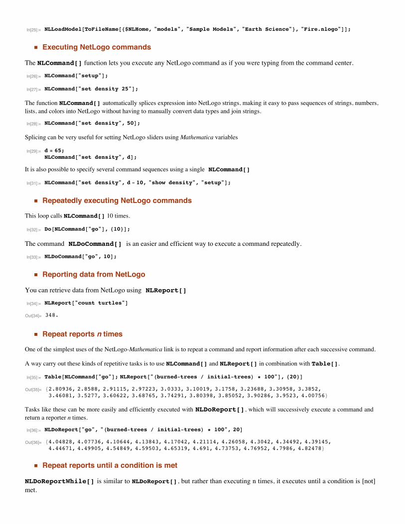
In[44]:= H* create a color for each density *LnumColors = Length@densitiesD;densityColors = Table@Blend@8 81, Yellow<, 8numColors, Red<<, nD, 8n, numColors<D;H* makes each run equal length *LmaxSteps = Max@Length êü fireDataD;completedData = HPadRight@Ò, maxSteps, Last@ÒDD &L êü fireData;

ListLinePlot@Thread@Tooltip@completedData, densitiesDD, PlotStyle Ø densityColors,AxesLabel Ø 8"Time", "% Burned"<, PlotLabel Ø "Burn time series with varying tree densities"D

Out[48]=

100 200 300 400 500Time

20

40

60

80

100% Burned

Burn time series with varying tree densities

Each line represents the time dynamics of the Forest Fire model run with a different density. Lines are colored by density, ranging fromlow (yellow) to high (red). Put your mouse over a line to see a tooltip of the density used in each run.

Ë Plot the phase transition by plotting how (final states) % burned vary with density

In[49]:= H*pair each density with the final % burned from each run *LfinalStates = Map@Last, fireDataD;densityBurnedPairs = Transpose@8densities, finalStates<D;ListPlot@densityBurnedPairs, AxesLabel Ø 8"Density", "Final % Burned"<,PlotRange Ø 80, 100<, PlotLabel Ø "Phase transition in the forest fire model"D

Out[51]=

50 55 60 65 70Density

20

40

60

80

100Final% Burned

Phase transition in the forest fire model

Comparing Empirical and Analytic Distributions in GasLabUse the Histograms package

In[52]:= Needs@"Histograms`"D;

Load GasLab Free Gas, set it up with 100 particles, and let it run for a little while

In[53]:= NLLoadModel@ToFileName@8$NLHome, "models", "Sample Models", "Chemistry & Physics", "GasLab"<, "GasLab Free Gas.nlogo"D

D;NLCommand@"set number-of-particles 100", "no-display", "setup"D;NLDoCommandWhile@"go", "ticks < 20"D;

ü Reporting lists of values from NetLogo

The NetLogo-Mathematica link automatically converts NetLogo lists into Mathematica lists.This is can be useful for examining distributions. Here, we execute the model for 20 "ticks" and report back the speed of each particle

In[56]:= NLReport@"@speedD of particles"DOut[56]= 86.14497, 16.0599, 14.4474, 11.5773, 2.9599, 8.51861, 13.4426, 14.6648, 15.0931,

8.76198, 11.7609, 10.7949, 15.5858, 6.40335, 7.99741, 5.87875, 9.1826, 5.27631, 0.330552,4.31802, 4.31481, 19.2086, 11.1245, 13.396, 1.17052, 5.54085, 8.67902, 5.80415, 9.94188,13.2382, 8.05882, 13.9302, 4.91512, 6.93483, 16.6934, 11.2409, 2.64028, 13.4318, 13.8411,5.58478, 23.0854, 7.92441, 3.87141, 5.89671, 11.0728, 9.70197, 5.60601, 11.267, 8.07937,9.47026, 9.95346, 7.22083, 10., 6.81408, 7.80311, 9.19168, 4.4496, 1.93631, 4.41357,4.73173, 12.7081, 11.985, 10.642, 8.04661, 14.7984, 1.80673, 8.94562, 13.0233, 8.7052,17.9542, 8.91671, 7.48248, 4.25952, 9.45168, 12.7482, 9.23808, 5.00108, 8.33814, 7.77296,6.42023, 6.57857, 10., 4.77582, 7.1417, 9.66377, 9.94719, 6.92942, 10., 9.69742, 10.,12.2595, 9.18922, 1.51168, 3.05593, 11.2862, 11.8339, 20.0552, 6.9563, 2.91476, 10.5254<

Ë Symbolic computing and NetLogo: validating the Maxwell-Boltzmann distribution

Set up the model with 500 particles and collect 40 readings of each particle's speed, every 50 steps.

In[57]:= NLCommand@"set number-of-particles 500", "no-display", "setup"D;speeds = Flatten@ NLDoReport@"repeat 50 @goD", "@speedD of particles", 40D D;

Compare distribution of speeds with the theoretical Maxwell-Boltzmann distribution for a 2D gas, BHvL = v ‰-mv2

2 k T

In[59]:= 8k, m, T< = 81, 1, NLReport@"mean @energyD of particles"D<;

In[60]:= B@v_D := v E-m v2

2 k T ;

normalizer = ‡0

¶

B@vD „v;

theoretical = PlotB B@vDnormalizer

, 8v, 0, Max@speedsD<, PlotStyle Ø 8Darker@RedD, Thickness@0.008D<F;empirical = Histogram@speeds, HistogramScale Ø 1D;Show@empirical, theoretical,PlotLabel Ø "GasLab energy distribution and the Maxwell|Boltzmann distribution"D

Out[64]=

5 10 15 20 25 30

0.02

0.04

0.06

0.08

GasLab energy distribution and the Maxwell|Boltzmann distribution

Screenshot Sequences with Termites

Screenshot Sequences with TermitesIn[65]:= NLLoadModel@ToFileName@8$NLHome, "models", "Sample Models", "Biology"<, "Termites.nlogo"DD;

NLCommand@"setup", "no-display"D;

ü Capturing NetLogo patch colors

One can use NLGetPatches[] to get values from patches.In this case we are reporting back NetLogo patch colors.

In[67]:= ArrayPlot@NLGetPatches@"pcolor"D, ColorRules Ø 80. Ø Black, 45. Ø Yellow<D

Out[67]=

Ë Collecting multiple "screenshots"

CaptureTermiteProgress[] asks the turtles to "go" 20 times and take a "screenshot" using NLGetPatches[].

In[68]:= CaptureTermiteProgress@D := Module@8<,NLDoCommand@"ask turtles @goD", 20D;NLGetPatches@"pcolor"D

D;Set up the model, and repeat CaptureTermiteProgress[] six times to capture several "screen shots".

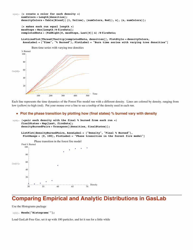
In[69]:= NLCommand@"setup"DpatchShots = Table@CaptureTermiteProgress@D, 86<D;renderedShots = Map@Rasterize@ArrayPlot@Ò, ColorRules Ø 80. Ø Black, 45. Ø Yellow<DD &, patchShotsD;

Ë Display screenshot simultaneously in a grid

Display each consecutive screenshot simultaneously in a grid

GraphicsGrid@Partition@renderedShots, 3D, ImageSize Ø 500D

Out[72]=

Ë Animate screenshots

Animate the screenshots and replay the model backwards and forwards

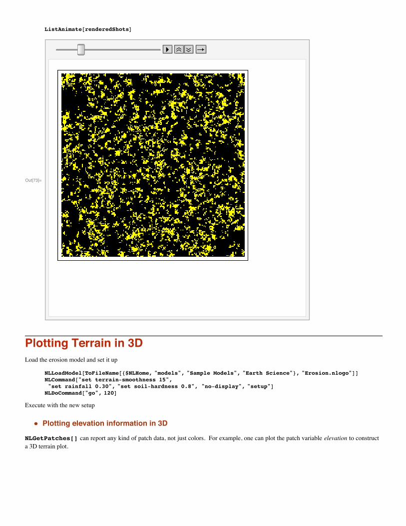
ListAnimate@renderedShotsD

Out[73]=

Plotting Terrain in 3DLoad the erosion model and set it up

NLLoadModel@ToFileName@8$NLHome, "models", "Sample Models", "Earth Science"<, "Erosion.nlogo"DDNLCommand@"set terrain-smoothness 15","set rainfall 0.30", "set soil-hardness 0.8", "no-display", "setup"DNLDoCommand@"go", 120D

Execute with the new setup

Ë Plotting elevation information in 3D

NLGetPatches[] can report any kind of patch data, not just colors. For example, one can plot the patch variable elevation to constructa 3D terrain plot.

In[77]:= elevations = NLGetPatches@"elevation"D;ListPlot3D@elevations, Mesh Ø None, ColorFunction Ø "Topographic",Mesh Ø None, Axes Ø None, Boxed Ø False, ViewPoint Ø 80.8, -1.5, 2.9<D

Out[78]=

Plotting Networks with Preferential AttachmentLoad the Preferential Attachment model

In[79]:= NLLoadModel@ToFileName@8$NLHome, "models", "Sample Models", "Networks"<, "Preferential Attachment.nlogo"DD

Set up the model and generate about 2000 nodes.

In[80]:= NLCommand@"setup set layout? false set plot? false no-display"D;NLDoCommand@"go", 2000D;

ü Capturing Graphs in NetLogo

Capture the network with NLGetGraph[]

In[82]:= network = NLGetGraph@"links"D;

By default, NLGetGraph[] uses the generic link breed, links

In[83]:= network = NLGetGraph@D;

NLGetGraph[] returns a list of rules of the form outNodeØ inNode, which can be used by NetLogo's visualization functions, whereoutNode and inNode are the who numbers of agents in the network.

In[84]:= Short@networkDOut[84]//Short=

8719 Ø 1846, 276 Ø 313, 117 Ø 1006, 11 Ø 1780, 21 Ø 1945, 6 Ø 1244,á1989à, 113 Ø 170, 466 Ø 1236, 63 Ø 1489, 715 Ø 980, 166 Ø 334, 1625 Ø 1972<

Ë Visualizing NetLogo graphs

Let Mathematica automatically pick a layout.

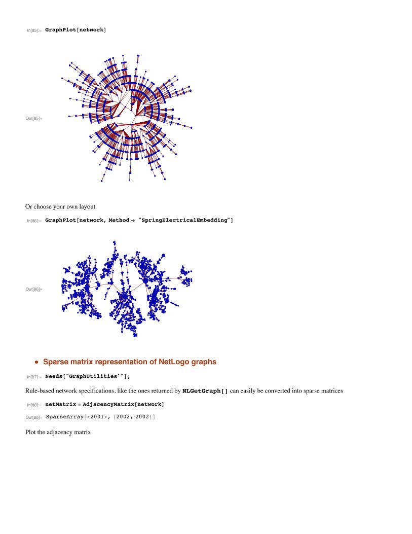
In[85]:= GraphPlot@networkD

Out[85]=

Or choose your own layout

In[86]:= GraphPlot@network, Method Ø "SpringElectricalEmbedding"D

Out[86]=

Ë Sparse matrix representation of NetLogo graphs

In[87]:= Needs@"GraphUtilities`"D;

Rule-based network specifications, like the ones returned by NLGetGraph[] can easily be converted into sparse matrices

In[88]:= netMatrix = AdjacencyMatrix@networkDOut[88]= SparseArray@<2001>, 82002, 2002<D

Plot the adjacency matrix

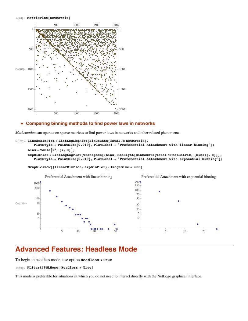
In[89]:= MatrixPlot@netMatrixD

Out[89]=

1 500 1000 1500 2002

1

500

1000

1500

2002

1 500 1000 1500 20021

500

1000

1500

2002

Ë Comparing binning methods to find power laws in networks

Mathematica can operate on sparse matrices to find power laws in networks and other related phenomena

In[107]:= linearBinPlot = ListLogLogPlot@BinCounts@Total êü netMatrixD,PlotStyle Ø PointSize@0.019D, PlotLabel Ø "Preferential Attachment with linear binning"D;

bins = TableA2i, 8i, 8<E;expBinPlot = ListLogLogPlot@Transpose@8bins, PadRight@BinCounts@Total êü netMatrix, 8bins<D, 8D<D,

PlotStyle Ø PointSize@0.019D, PlotLabel Ø "Preferential Attachment with expoential binning"D;GraphicsRow@8linearBinPlot, expBinPlot<, ImageSize Ø 600D

Out[110]=

5 10 20 50

510

50100

5001000

Preferential Attachment with linear binning

5 10 20

10

100

50

20

200

30

15

150

70

Preferential Attachment with expoential binning

Advanced Features: Headless ModeTo begin in headless mode, use option HeadlessØTrue

In[94]:= NLStart@$NLHome, Headless Ø TrueD

This mode is preferable for situations in which you do not need to interact directly with the NetLogo graphical interface.