Embed Size (px)
Citation preview
APPENDIX
MATLAB SCRIPTS
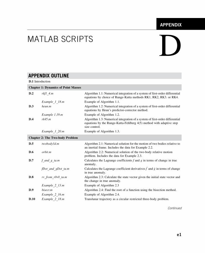
D APPENDIX OUTLINED.1 IntroductionChapter 1: Dynamics of Point Masses
D.2
rkf1_4.m Algorithm 1.1: Numerical integration of a system of first-order differentialequations by choice of Runge-Kutta methods RK1, RK2, RK3. or RK4.
Example_1_18.m
Example of Algorithm 1.1.D.3
heun.m Algorithm 1.2: Numerical integration of a system of first-order differentialequations by Heun’s predictor-corrector method.
Example 1.19.m
Example of Algorithm 1.2.D.4
rk45.m Algorithm 1.3: Numerical integration of a system of first-order differentialequations by the Runge-Kutta-Fehlberg 4(5) method with adaptive step
size control.
Example_1_20.m
Example of Algorithm 1.3.Chapter 2: The Two-body Problem
D.5
twobody3d.m Algorithm 2.1: Numerical solution for the motion of two bodies relative toan inertial frame. Includes the data for Example 2.2.
D.6
orbit.m Algorithm 2.2: Numerical solution of the two-body relative motionproblem. Includes the data for Example 2.3.
D.7
f_and_g_ta.m Calculates the Lagrange coefficients f and g in terms of change in trueanomaly.
fDot_and_gDot_ta.m
Calculates the Lagrange coefficient derivatives _f and _g in terms of changein true anomaly.
D.8
rv_from_r0v0_ta.m Algorithm 2.3: Calculate the state vector given the initial state vector andthe change in true anomaly.
Example_2_13.m
Example of Algorithm 2.3D.9
bisect.m Algorithm 2.4: Find the root of a function using the bisection method.Example_2_16.m
Example of Algorithm 2.4.D.10
Example_2_18.m Translunar trajectory as a circular restricted three-body problem.Continued
e1
e2 MATLAB scripts
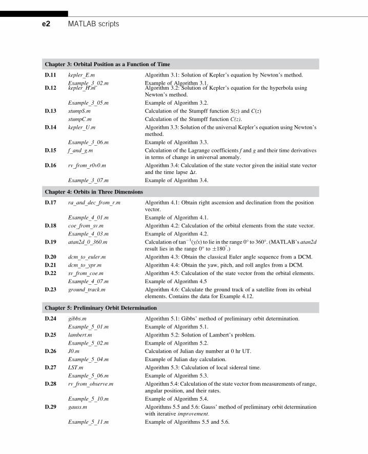
Chapter 3: Orbital Position as a Function of Time
D.11
kepler_E.m Algorithm 3.1: Solution of Kepler’s equation by Newton’s method.Example_3_02.m
Example of Algorithm 3.1. D.12 kepler_H.m Algorithm 3.2: Solution of Kepler’s equation for the hyperbola usingNewton’s method.
Example_3_05.m
Example of Algorithm 3.2.D.13
stumpS.m Calculation of the Stumpff function S(z) and C(z)stumpC.m
Calculation of the Stumpff function C(z).D.14
kepler_U.m Algorithm 3.3: Solution of the universal Kepler’s equation using Newton’smethod.
Example_3_06.m
Example of Algorithm 3.3.D.15
f_and_g.m Calculation of the Lagrange coefficients f and g and their time derivativesin terms of change in universal anomaly.
D.16
rv_from_r0v0.m Algorithm 3.4: Calculation of the state vector given the initial state vectorand the time lapse Δt.
Example_3_07.m Example of Algorithm 3.4.Chapter 4: Orbits in Three Dimensions
D.17
ra_and_dec_from_r.m Algorithm 4.1: Obtain right ascension and declination from the positionvector.
Example_4_01.m
Example of Algorithm 4.1.D.18
coe_from_sv.m Algorithm 4.2: Calculation of the orbital elements from the state vector.Example_4_03.m
Example of Algorithm 4.2.D.19
atan2d_0_360.m Calculation of tan�1(y/x) to lie in the range 0° to 360°. (MATLAB’s atan2dresult lies in the range 0° to �180°.)D.20
dcm_to_euler.m Algorithm 4.3: Obtain the classical Euler angle sequence from a DCM.D.21
dcm_to_ypr.m Algorithm 4.4: Obtain the yaw, pitch, and roll angles from a DCM.D.22
sv_from_coe.m Algorithm 4.5: Calculation of the state vector from the orbital elements.Example_4_07.m
Example of Algorithm 4.5D.23
ground_track.m Algorithm 4.6: Calculate the ground track of a satellite from its orbitalelements. Contains the data for Example 4.12.
Chapter 5: Preliminary Orbit Determination
D.24
gibbs.m Algorithm 5.1: Gibbs’ method of preliminary orbit determination.Example_5_01.m
Example of Algorithm 5.1.D.25
lambert.m Algorithm 5.2: Solution of Lambert’s problem.Example_5_02.m
Example of Algorithm 5.2.D.26
J0.m Calculation of Julian day number at 0 hr UT.Example_5_04.m
Example of Julian day calculation.D.27
LST.m Algorithm 5.3: Calculation of local sidereal time.Example_5_06.m
Example of Algorithm 5.3.D.28
rv_from_observe.m Algorithm 5.4: Calculation of the state vector frommeasurements of range,angular position, and their rates.
Example_5_10.m
Example of Algorithm 5.4.D.29
gauss.m Algorithms 5.5 and 5.6: Gauss’ method of preliminary orbit determinationwith iterative improvement.
Example_5_11.m
Example of Algorithms 5.5 and 5.6.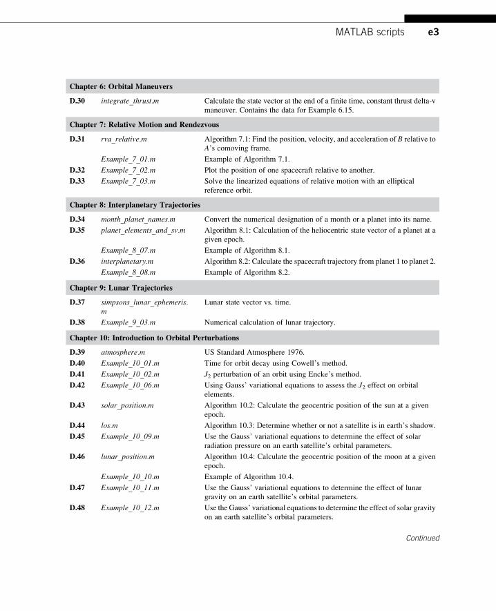
e3MATLAB scripts
Chapter 6: Orbital Maneuvers
D.30
integrate_thrust.m Calculate the state vector at the end of a finite time, constant thrust delta-vmaneuver. Contains the data for Example 6.15.
Chapter 7: Relative Motion and Rendezvous
D.31
rva_relative.m Algorithm 7.1: Find the position, velocity, and acceleration of B relative toA’s comoving frame.
Example_7_01.m
Example of Algorithm 7.1.D.32
Example_7_02.m Plot the position of one spacecraft relative to another.D.33
Example_7_03.m Solve the linearized equations of relative motion with an ellipticalreference orbit.
Chapter 8: Interplanetary Trajectories
D.34
month_planet_names.m Convert the numerical designation of a month or a planet into its name.D.35
planet_elements_and_sv.m Algorithm 8.1: Calculation of the heliocentric state vector of a planet at agiven epoch.
Example_8_07.m
Example of Algorithm 8.1.D.36
interplanetary.m Algorithm 8.2: Calculate the spacecraft trajectory from planet 1 to planet 2.Example_8_08.m
Example of Algorithm 8.2.Chapter 9: Lunar Trajectories
D.37
simpsons_lunar_ephemeris.mLunar state vector vs. time.
D.38
Example_9_03.m Numerical calculation of lunar trajectory.Chapter 10: Introduction to Orbital Perturbations
D.39
atmosphere.m US Standard Atmosphere 1976.D.40
Example_10_01.m Time for orbit decay using Cowell’s method.D.41
Example_10_02.m J2 perturbation of an orbit using Encke’s method.D.42
Example_10_06.m Using Gauss’ variational equations to assess the J2 effect on orbitalelements.
D.43
solar_position.m Algorithm 10.2: Calculate the geocentric position of the sun at a givenepoch.
D.44
los.m Algorithm 10.3: Determine whether or not a satellite is in earth’s shadow.D.45
Example_10_09.m Use the Gauss’ variational equations to determine the effect of solarradiation pressure on an earth satellite’s orbital parameters.
D.46
lunar_position.m Algorithm 10.4: Calculate the geocentric position of the moon at a givenepoch.
Example_10_10.m
Example of Algorithm 10.4.D.47
Example_10_11.m Use the Gauss’ variational equations to determine the effect of lunargravity on an earth satellite’s orbital parameters.
D.48
Example_10_12.m Use the Gauss’ variational equations to determine the effect of solar gravityon an earth satellite’s orbital parameters.
Continued
e4 MATLAB scripts
Chapter 11: Rigid Body Dynamics
D.49
dcm_from_q.m Algorithm 11.1: Calculate the direction cosine matrix from the quaternion.D.50
q_from_dcm.m Algorithm 11.2: Calculate the quaternion from the direction cosine matrix.D.51
quat_rotate.m Quaternion vector rotation operation (Eq. 11.160).D.52
Example_11_26.m Solution of the spinning top problem.Chapter 12: Spacecraft Attitude Dynamics
Chapter 13: Rocket Vehicle Dynamics
D.53
Example_13_03.m Example 11.3: Calculation of a gravity turn trajectory.D.1 INTRODUCTIONThis appendix lists MATLAB scripts that implement all the numbered algorithms presented throughout
the text. The programs use only the most basic features of MATLAB and are liberally commented so as
to make reading the code as easy as possible. To “drive” the various algorithms, we can use MATLAB
to create graphical user interfaces (GUIs). However, in the interest of simplicity and keeping our focus
on the algorithms rather than elegant programming techniques, GUIs were not developed. Furthermore,
the scripts do not use files to import and export data. Data are defined in declaration statements within
the scripts. All output is to the screen (i.e., to the MATLAB Command Window). It is hoped that in-
terested students will embellish these simple scripts or use them as a springboard toward generating
their own programs.
Each algorithm is illustrated by a MATLAB coding of a related example problem in the text. The
actual output of each of these examples is also listed. These programs are presented solely as an alter-
native to carrying out otherwise lengthy hand computations and are intended for academic use only.
They are all based exclusively on the introductory material presented in this text. Should it be necessary
to do so, it is a fairly simple matter to translate these programs into other software languages.
It would be helpful to have MATLAB documentation at hand. There are many practical references
on the subject in bookstores and online, including those at The MathWorks website (www.mathworks.
com).
CHAPTER 1: DYNAMICS OF POINT MASSES
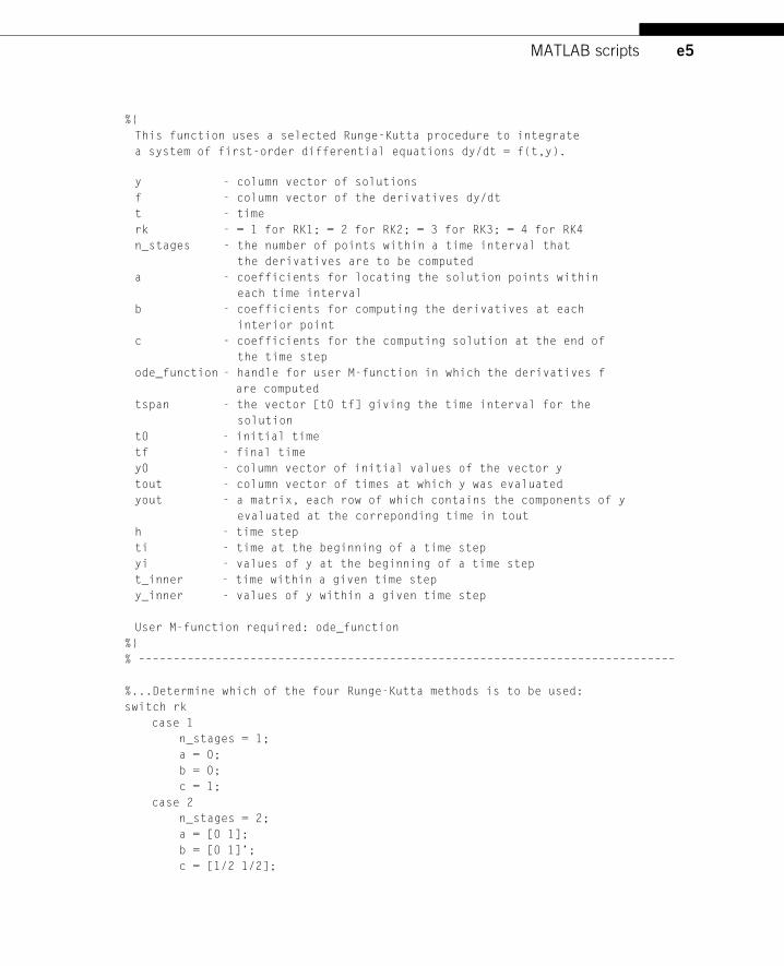
D.2 ALGORITHM 1.1: NUMERICAL INTEGRATION BY RUNGE-KUTTAMETHODS RK1, RK2, RK3, OR RK4FUNCTION FILE rkf1_4.m
% ������������������������������������������������������������function [tout, yout] = rk1_4(ode_function, tspan, y0, h, rk)
% ������������������������������������������������������������
e5MATLAB scripts
%{
This function uses a selected Runge-Kutta procedure to integrate
a system of first-order differential equations dy/dt = f(t,y).
y - column vector of solutions
f - column vector of the derivatives dy/dt
t - time
rk - = 1 for RK1; = 2 for RK2; = 3 for RK3; = 4 for RK4
n_stages - the number of points within a time interval that
the derivatives are to be computed
a - coefficients for locating the solution points within
each time interval
b - coefficients for computing the derivatives at each
interior point
c - coefficients for the computing solution at the end of
the time step
ode_function - handle for user M-function in which the derivatives f
are computed
tspan - the vector [t0 tf] giving the time interval for the
solution
t0 - initial time
tf - final time
y0 - column vector of initial values of the vector y
tout - column vector of times at which y was evaluated
yout - a matrix, each row of which contains the components of y
evaluated at the correponding time in tout
h - time step
ti - time at the beginning of a time step
yi - values of y at the beginning of a time step
t_inner - time within a given time step
y_inner - values of y within a given time step
User M-function required: ode_function
%}
% –––––––––––––––––––––––––––––––––––––––––––––––––––––––––––––––––––––––––––––
%...Determine which of the four Runge-Kutta methods is to be used:
switch rk
case 1
n_stages = 1;
a = 0;
b = 0;
c = 1;
case 2
n_stages = 2;
a = [0 1];
b = [0 1]’;
c = [1/2 1/2];
e6 MATLAB scripts
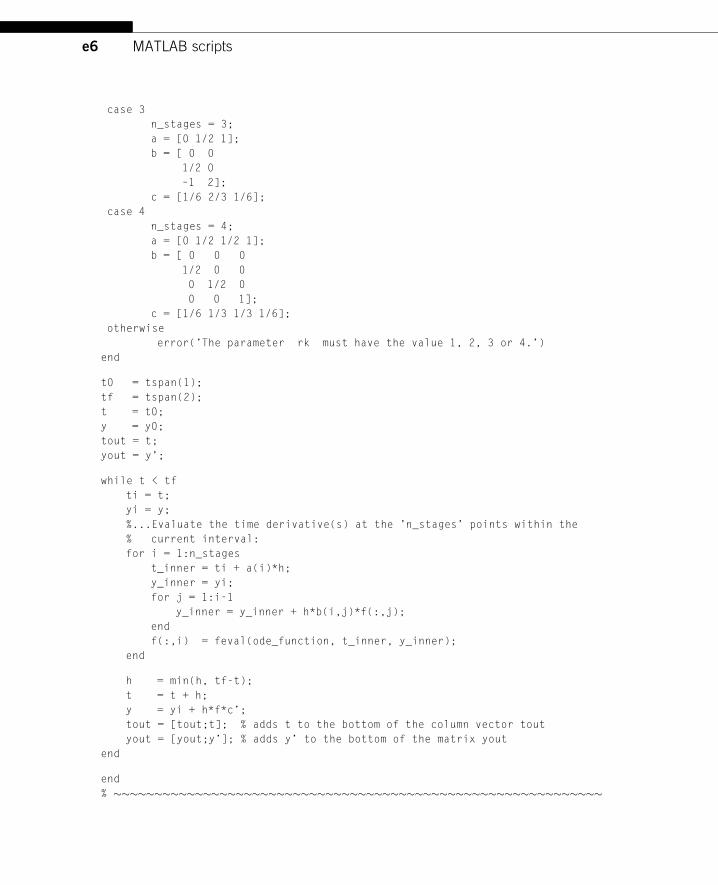
case 3
n_stages = 3;
a = [0 1/2 1];
b = [ 0 0
1/2 0
–1 2];
c = [1/6 2/3 1/6];
case 4
n_stages = 4;
a = [0 1/2 1/2 1];
b = [ 0 0 0
1/2 0 0
0 1/2 0
0 0 1];
c = [1/6 1/3 1/3 1/6];
otherwise
error(’The parameter rk must have the value 1, 2, 3 or 4.’)
end
t0 = tspan(1);
tf = tspan(2);
t = t0;
y = y0;
tout = t;
yout = y’;
while t < tf
ti = t;
yi = y;
%...Evaluate the time derivative(s) at the ’n_stages’ points within the
% current interval:
for i = 1:n_stages
t_inner = ti + a(i)*h;
y_inner = yi;
for j = 1:i-1
y_inner = y_inner + h*b(i,j)*f(:,j);
end
f(:,i) = feval(ode_function, t_inner, y_inner);
end
h = min(h, tf-t);
t = t + h;
y = yi + h*f*c’;
tout = [tout;t]; % adds t to the bottom of the column vector tout
yout = [yout;y’]; % adds y’ to the bottom of the matrix yout
end
end
% ������������������������������������������������������������
e7MATLAB scripts
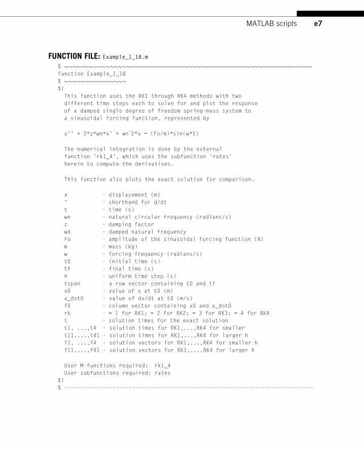
FUNCTION FILE: Example_1_18.m
% ������������������������������������������������������������function Example_1_18
% ���������������%{
This function uses the RK1 through RK4 methods with two
different time steps each to solve for and plot the response
of a damped single degree of freedom spring-mass system to
a sinusoidal forcing function, represented by
x’’ + 2*z*wn*x’ + wn 2̂*x = (Fo/m)*sin(w*t)
The numerical integration is done by the external
function ’rk1_4’, which uses the subfunction ’rates’
herein to compute the derivatives.
This function also plots the exact solution for comparison.
x - displacement (m)
’ - shorthand for d/dt
t - time (s)
wn - natural circular frequency (radians/s)
z - damping factor
wd - damped natural frequency
Fo - amplitude of the sinusoidal forcing function (N)
m - mass (kg)
w - forcing frequency (radians/s)
t0 - initial time (s)
tf - final time (s)
h - uniform time step (s)
tspan - a row vector containing t0 and tf
x0 - value of x at t0 (m)
x_dot0 - value of dx/dt at t0 (m/s)
f0 - column vector containing x0 and x_dot0
rk - = 1 for RK1; = 2 for RK2; = 3 for RK3; = 4 for RK4
t - solution times for the exact solution
t1, ...,t4 - solution times for RK1,...,RK4 for smaller
t11,...,t41 - solution times for RK1,...,RK4 for larger h
f1, ...,f4 - solution vectors for RK1,...,RK4 for smaller h
f11,...,f41 - solution vectors for RK1,...,RK4 for larger h
User M-functions required: rk1_4
User subfunctions required: rates
%}
% –––––––––––––––––––––––––––––––––––––––––––––––––––––––––––––––––––––––––––––
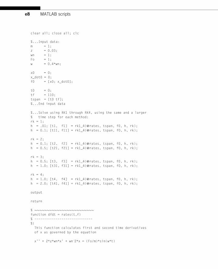
e8 MATLAB scripts
clear all; close all; clc
%...Input data:
m = 1;
z = 0.03;
wn = 1;
Fo = 1;
w = 0.4*wn;
x0 = 0;
x_dot0 = 0;
f0 = [x0; x_dot0];
t0 = 0;
tf = 110;
tspan = [t0 tf];
%...End input data
%...Solve using RK1 through RK4, using the same and a larger
% time step for each method:
rk = 1;
h = .01; [t1, f1] = rk1_4(@rates, tspan, f0, h, rk);
h = 0.1; [t11, f11] = rk1_4(@rates, tspan, f0, h, rk);
rk = 2;
h = 0.1; [t2, f2] = rk1_4(@rates, tspan, f0, h, rk);
h = 0.5; [t21, f21] = rk1_4(@rates, tspan, f0, h, rk);
rk = 3;
h = 0.5; [t3, f3] = rk1_4(@rates, tspan, f0, h, rk);
h = 1.0; [t31, f31] = rk1_4(@rates, tspan, f0, h, rk);
rk = 4;
h = 1.0; [t4, f4] = rk1_4(@rates, tspan, f0, h, rk);
h = 2.0; [t41, f41] = rk1_4(@rates, tspan, f0, h, rk);
output
return
% ������������������������function dfdt = rates(t,f)
% ––––––––––––––––––––––––––––––
%{
This function calculates first and second time derivatives
of x as governed by the equation
x’’ + 2*z*wn*x’ + wn 2̂*x = (Fo/m)*sin(w*t)
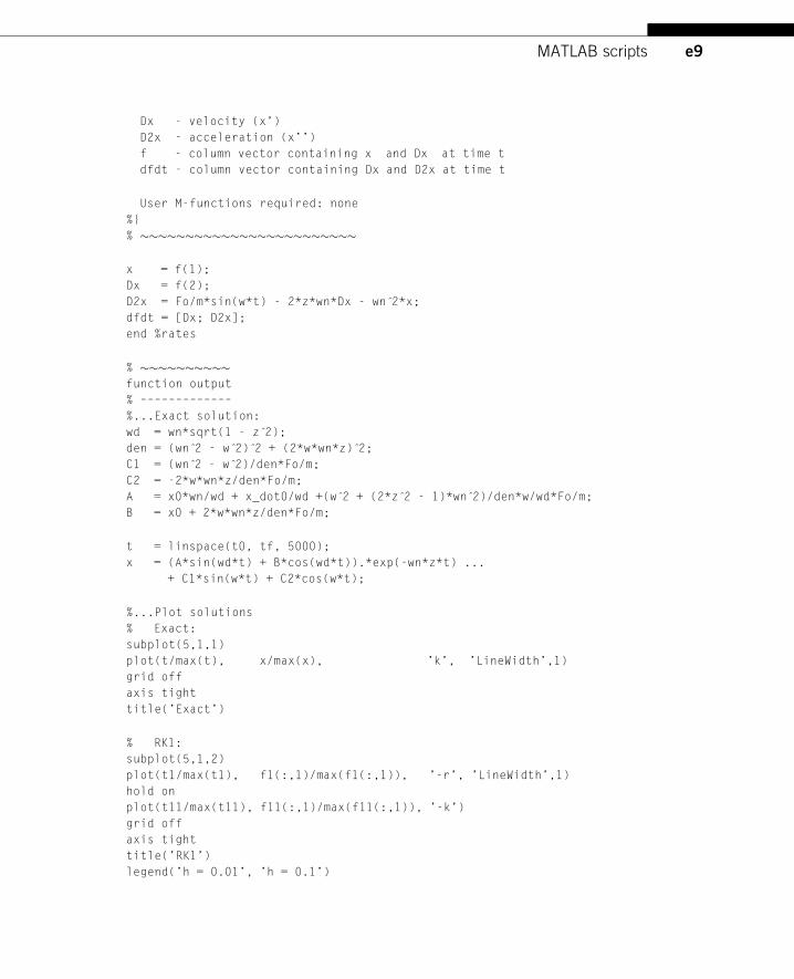
e9MATLAB scripts
Dx - velocity (x’)
D2x - acceleration (x’’)
f - column vector containing x and Dx at time t
dfdt - column vector containing Dx and D2x at time t
User M-functions required: none
%}
% ������������������������
x = f(1);
Dx = f(2);
D2x = Fo/m*sin(w*t) - 2*z*wn*Dx - wn 2̂*x;
dfdt = [Dx; D2x];
end %rates
% ����������function output
% –––––––––––––
%...Exact solution:
wd = wn*sqrt(1 - z 2̂);
den = (wn 2̂ - w 2̂) 2̂ + (2*w*wn*z) 2̂;
C1 = (wn 2̂ - w 2̂)/den*Fo/m;
C2 = -2*w*wn*z/den*Fo/m;
A = x0*wn/wd + x_dot0/wd +(w 2̂ + (2*z 2̂ - 1)*wn 2̂)/den*w/wd*Fo/m;
B = x0 + 2*w*wn*z/den*Fo/m;
t = linspace(t0, tf, 5000);
x = (A*sin(wd*t) + B*cos(wd*t)).*exp(-wn*z*t) ...
+ C1*sin(w*t) + C2*cos(w*t);
%...Plot solutions
% Exact:
subplot(5,1,1)
plot(t/max(t), x/max(x), ’k’, ’LineWidth’,1)
grid off
axis tight
title(’Exact’)
% RK1:
subplot(5,1,2)
plot(t1/max(t1), f1(:,1)/max(f1(:,1)), ’-r’, ’LineWidth’,1)
hold on
plot(t11/max(t11), f11(:,1)/max(f11(:,1)), ’-k’)
grid off
axis tight
title(’RK1’)
legend(’h = 0.01’, ’h = 0.1’)
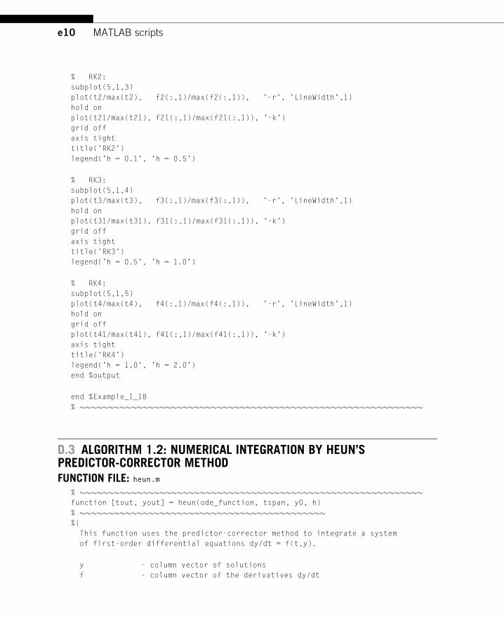
e10 MATLAB scripts
% RK2:
subplot(5,1,3)
plot(t2/max(t2), f2(:,1)/max(f2(:,1)), ’-r’, ’LineWidth’,1)
hold on
plot(t21/max(t21), f21(:,1)/max(f21(:,1)), ’-k’)
grid off
axis tight
title(’RK2’)
legend(’h = 0.1’, ’h = 0.5’)
% RK3:
subplot(5,1,4)
plot(t3/max(t3), f3(:,1)/max(f3(:,1)), ’-r’, ’LineWidth’,1)
hold on
plot(t31/max(t31), f31(:,1)/max(f31(:,1)), ’-k’)
grid off
axis tight
title(’RK3’)
legend(’h = 0.5’, ’h = 1.0’)
% RK4:
subplot(5,1,5)
plot(t4/max(t4), f4(:,1)/max(f4(:,1)), ’-r’, ’LineWidth’,1)
hold on
grid off
plot(t41/max(t41), f41(:,1)/max(f41(:,1)), ’-k’)
axis tight
title(’RK4’)
legend(’h = 1.0’, ’h = 2.0’)
end %output
end %Example_1_18
% ������������������������������������������������������������
D.3 ALGORITHM 1.2: NUMERICAL INTEGRATION BY HEUN’SPREDICTOR-CORRECTOR METHODFUNCTION FILE: heun.m
% ������������������������������������������������������������function [tout, yout] = heun(ode_function, tspan, y0, h)
% �������������������������������������������%{
This function uses the predictor-corrector method to integrate a system
of first-order differential equations dy/dt = f(t,y).
y - column vector of solutions
f - column vector of the derivatives dy/dt
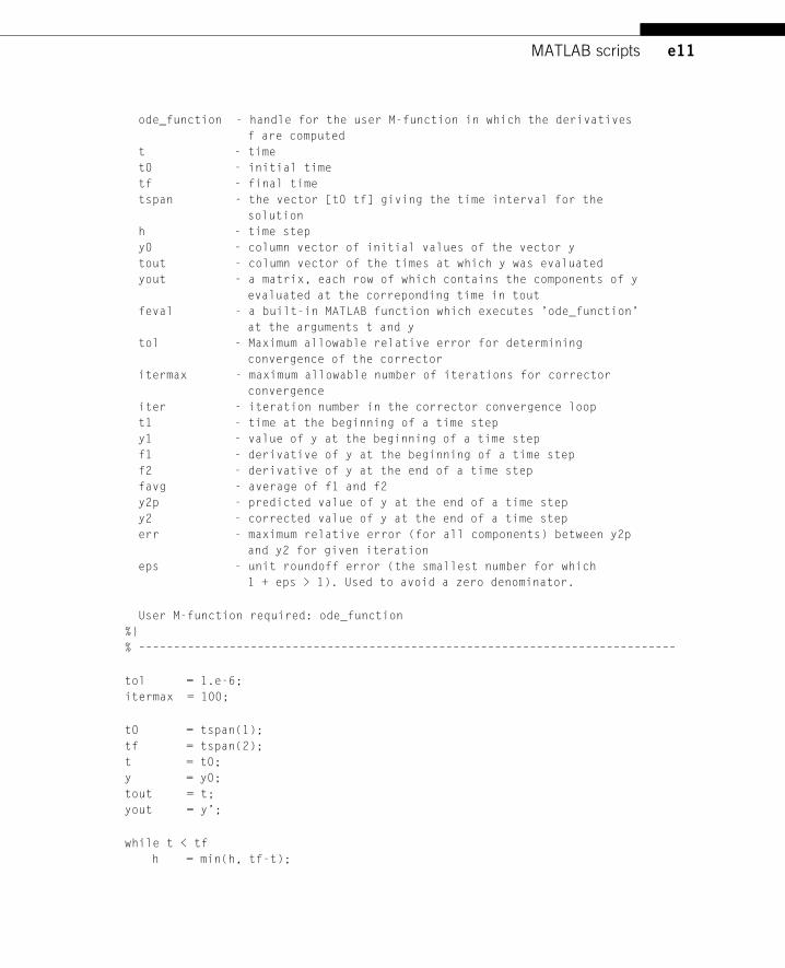
e11MATLAB scripts
ode_function - handle for the user M-function in which the derivatives
f are computed
t - time
t0 - initial time
tf - final time
tspan - the vector [t0 tf] giving the time interval for the
solution
h - time step
y0 - column vector of initial values of the vector y
tout - column vector of the times at which y was evaluated
yout - a matrix, each row of which contains the components of y
evaluated at the correponding time in tout
feval - a built-in MATLAB function which executes ’ode_function’
at the arguments t and y
tol - Maximum allowable relative error for determining
convergence of the corrector
itermax - maximum allowable number of iterations for corrector
convergence
iter - iteration number in the corrector convergence loop
t1 - time at the beginning of a time step
y1 - value of y at the beginning of a time step
f1 - derivative of y at the beginning of a time step
f2 - derivative of y at the end of a time step
favg - average of f1 and f2
y2p - predicted value of y at the end of a time step
y2 - corrected value of y at the end of a time step
err - maximum relative error (for all components) between y2p
and y2 for given iteration
eps - unit roundoff error (the smallest number for which
1 + eps > 1). Used to avoid a zero denominator.
User M-function required: ode_function
%}
% –––––––––––––––––––––––––––––––––––––––––––––––––––––––––––––––––––––––––––––
tol = 1.e-6;
itermax = 100;
t0 = tspan(1);
tf = tspan(2);
t = t0;
y = y0;
tout = t;
yout = y’;
while t < tf
h = min(h, tf-t);
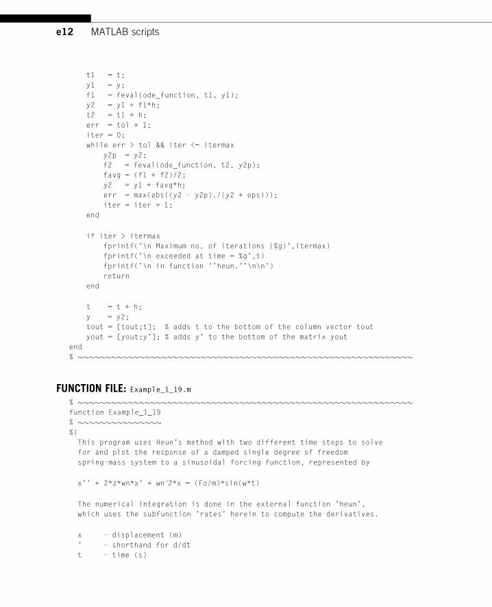
e12 MATLAB scripts
t1 = t;
y1 = y;
f1 = feval(ode_function, t1, y1);
y2 = y1 + f1*h;
t2 = t1 + h;
err = tol + 1;
iter = 0;
while err > tol && iter <= itermax
y2p = y2;
f2 = feval(ode_function, t2, y2p);
favg = (f1 + f2)/2;
y2 = y1 + favg*h;
err = max(abs((y2 - y2p)./(y2 + eps)));
iter = iter + 1;
end
if iter > itermax
fprintf(’\n Maximum no. of iterations (%g)’,itermax)
fprintf(’\n exceeded at time = %g’,t)
fprintf(’\n in function ’’heun.’’\n\n’)
return
end
t = t + h;
y = y2;
tout = [tout;t]; % adds t to the bottom of the column vector tout
yout = [yout;y’]; % adds y’ to the bottom of the matrix yout
end
% ������������������������������������������������������������
FUNCTION FILE: Example_1_19.m
% ������������������������������������������������������������function Example_1_19
% ���������������%{
This program uses Heun’s method with two different time steps to solve
for and plot the response of a damped single degree of freedom
spring-mass system to a sinusoidal forcing function, represented by
x’’ + 2*z*wn*x’ + wn 2̂*x = (Fo/m)*sin(w*t)
The numerical integration is done in the external function ’heun’,
which uses the subfunction ’rates’ herein to compute the derivatives.
x - displacement (m)
’ - shorthand for d/dt
t - time (s)
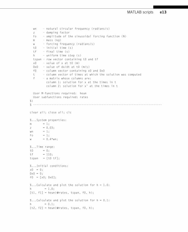
e13MATLAB scripts
wn - natural circular frequency (radians/s)
z - damping factor
Fo - amplitude of the sinusoidal forcing function (N)
m - mass (kg)
w - forcing frequency (radians/s)
t0 - initial time (s)
tf - final time (s)
h - uniform time step (s)
tspan - row vector containing t0 and tf
x0 - value of x at t0 (m)
Dx0 - value of dx/dt at t0 (m/s)
f0 - column vector containing x0 and Dx0
t - column vector of times at which the solution was computed
f - a matrix whose columns are:
column 1: solution for x at the times in t
column 2: solution for x’ at the times in t
User M-functions required: heun
User subfunctions required: rates
%}
% –––––––––––––––––––––––––––––––––––––––––––––––––––––––––––––––––––––––––––––
clear all; close all; clc
%...System properties:
m = 1;
z = 0.03;
wn = 1;
Fo = 1;
w = 0.4*wn;
%...Time range:
t0 = 0;
tf = 110;
tspan = [t0 tf];
%...Initial conditions:
x0 = 0;
Dx0 = 0;
f0 = [x0; Dx0];
%...Calculate and plot the solution for h = 1.0:
h = 1.0;
[t1, f1] = heun(@rates, tspan, f0, h);
%...Calculate and plot the solution for h = 0.1:
h = 0.1;
[t2, f2] = heun(@rates, tspan, f0, h);
e14 MATLAB scripts
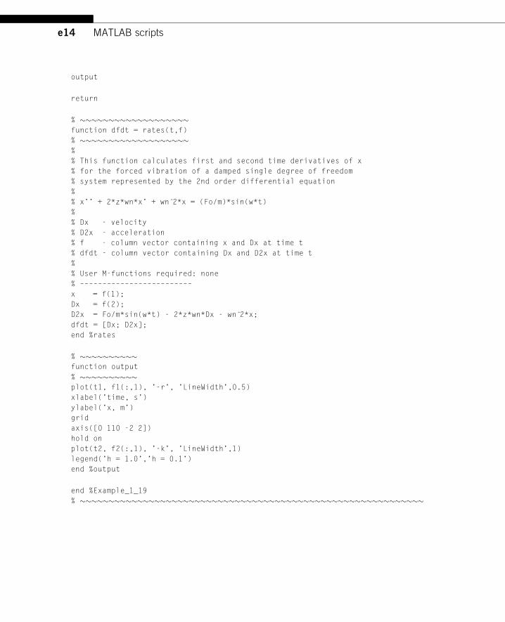
output
return
% �������������������function dfdt = rates(t,f)
% �������������������%
% This function calculates first and second time derivatives of x
% for the forced vibration of a damped single degree of freedom
% system represented by the 2nd order differential equation
%
% x’’ + 2*z*wn*x’ + wn 2̂*x = (Fo/m)*sin(w*t)
%
% Dx - velocity
% D2x - acceleration
% f - column vector containing x and Dx at time t
% dfdt - column vector containing Dx and D2x at time t
%
% User M-functions required: none
% –––––––––––––––––––––––––
x = f(1);
Dx = f(2);
D2x = Fo/m*sin(w*t) - 2*z*wn*Dx - wn 2̂*x;
dfdt = [Dx; D2x];
end %rates
% ����������function output
% ����������plot(t1, f1(:,1), ’-r’, ’LineWidth’,0.5)
xlabel(’time, s’)
ylabel(’x, m’)
grid
axis([0 110 -2 2])
hold on
plot(t2, f2(:,1), ’-k’, ’LineWidth’,1)
legend(’h = 1.0’,’h = 0.1’)
end %output
end %Example_1_19
% ������������������������������������������������������������
e15MATLAB scripts
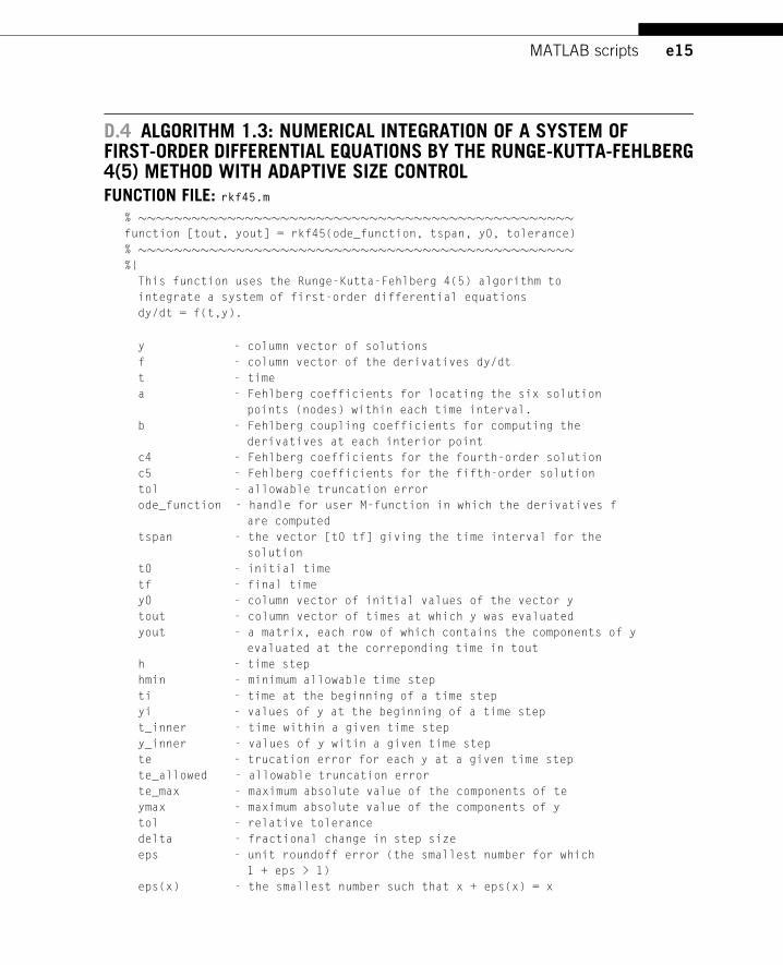
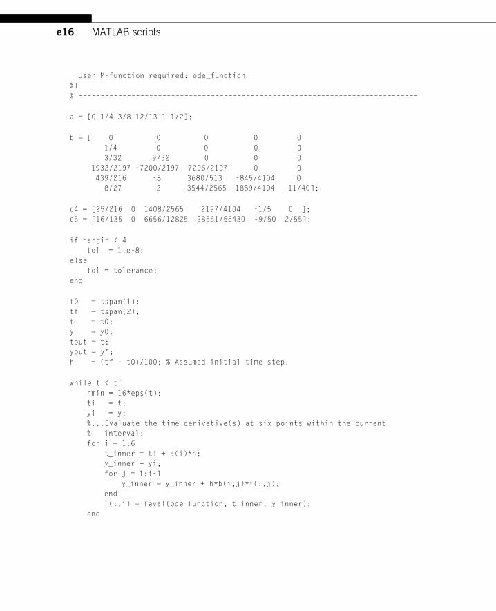
D.4 ALGORITHM 1.3: NUMERICAL INTEGRATION OF A SYSTEM OFFIRST-ORDER DIFFERENTIAL EQUATIONS BY THE RUNGE-KUTTA-FEHLBERG4(5) METHOD WITH ADAPTIVE SIZE CONTROLFUNCTION FILE: rkf45.m
% �������������������������������������������������function [tout, yout] = rkf45(ode_function, tspan, y0, tolerance)
% �������������������������������������������������%{
This function uses the Runge-Kutta-Fehlberg 4(5) algorithm to
integrate a system of first-order differential equations
dy/dt = f(t,y).
y - column vector of solutions
f - column vector of the derivatives dy/dt
t - time
a - Fehlberg coefficients for locating the six solution
points (nodes) within each time interval.
b - Fehlberg coupling coefficients for computing the
derivatives at each interior point
c4 - Fehlberg coefficients for the fourth-order solution
c5 - Fehlberg coefficients for the fifth-order solution
tol - allowable truncation error
ode_function - handle for user M-function in which the derivatives f
are computed
tspan - the vector [t0 tf] giving the time interval for the
solution
t0 - initial time
tf - final time
y0 - column vector of initial values of the vector y
tout - column vector of times at which y was evaluated
yout - a matrix, each row of which contains the components of y
evaluated at the correponding time in tout
h - time step
hmin - minimum allowable time step
ti - time at the beginning of a time step
yi - values of y at the beginning of a time step
t_inner - time within a given time step
y_inner - values of y witin a given time step
te - trucation error for each y at a given time step
te_allowed - allowable truncation error
te_max - maximum absolute value of the components of te
ymax - maximum absolute value of the components of y
tol - relative tolerance
delta - fractional change in step size
eps - unit roundoff error (the smallest number for which
1 + eps > 1)
eps(x) - the smallest number such that x + eps(x) = x
e16 MATLAB scripts
User M-function required: ode_function
%}
% –––––––––––––––––––––––––––––––––––––––––––––––––––––––––––––––––––––––––––––
a = [0 1/4 3/8 12/13 1 1/2];
b = [ 0 0 0 0 0
1/4 0 0 0 0
3/32 9/32 0 0 0
1932/2197 -7200/2197 7296/2197 0 0
439/216 -8 3680/513 -845/4104 0
-8/27 2 -3544/2565 1859/4104 -11/40];
c4 = [25/216 0 1408/2565 2197/4104 -1/5 0 ];
c5 = [16/135 0 6656/12825 28561/56430 -9/50 2/55];
if nargin < 4
tol = 1.e-8;
else
tol = tolerance;
end
t0 = tspan(1);
tf = tspan(2);
t = t0;
y = y0;
tout = t;
yout = y’;
h = (tf - t0)/100; % Assumed initial time step.
while t < tf
hmin = 16*eps(t);
ti = t;
yi = y;
%...Evaluate the time derivative(s) at six points within the current
% interval:
for i = 1:6
t_inner = ti + a(i)*h;
y_inner = yi;
for j = 1:i-1
y_inner = y_inner + h*b(i,j)*f(:,j);
end
f(:,i) = feval(ode_function, t_inner, y_inner);
end
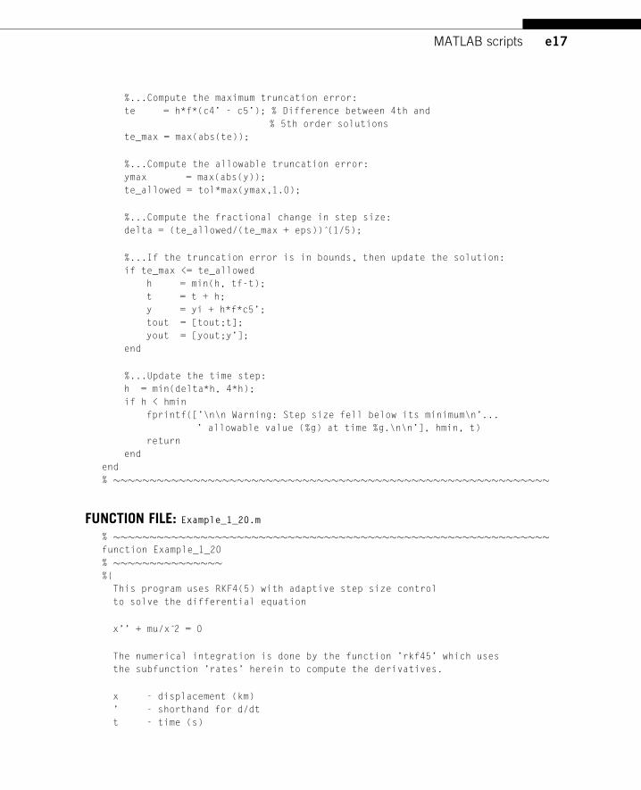
e17MATLAB scripts
%...Compute the maximum truncation error:
te = h*f*(c4’ - c5’); % Difference between 4th and
% 5th order solutions
te_max = max(abs(te));
%...Compute the allowable truncation error:
ymax = max(abs(y));
te_allowed = tol*max(ymax,1.0);
%...Compute the fractional change in step size:
delta = (te_allowed/(te_max + eps)) (̂1/5);
%...If the truncation error is in bounds, then update the solution:
if te_max <= te_allowed
h = min(h, tf-t);
t = t + h;
y = yi + h*f*c5’;
tout = [tout;t];
yout = [yout;y’];
end
%...Update the time step:
h = min(delta*h, 4*h);
if h < hmin
fprintf([’\n\n Warning: Step size fell below its minimum\n’...
’ allowable value (%g) at time %g.\n\n’], hmin, t)
return
end
end
% ������������������������������������������������������������
FUNCTION FILE: Example_1_20.m
% ������������������������������������������������������������function Example_1_20
% ���������������%{
This program uses RKF4(5) with adaptive step size control
to solve the differential equation
x’’ + mu/x 2̂ = 0
The numerical integration is done by the function ’rkf45’ which uses
the subfunction ’rates’ herein to compute the derivatives.
x - displacement (km)
’ - shorthand for d/dt
t - time (s)

e18 MATLAB scripts
mu - = go*RE 2̂ (km 3̂/s 2̂), where go is the sea level gravitational
acceleration and RE is the radius of the earth
x0 - initial value of x
v0 = initial value of the velocity (x’)
y0 - column vector containing x0 and v0
t0 - initial time
tf - final time
tspan - a row vector with components t0 and tf
t - column vector of the times at which the solution is found
f - a matrix whose columns are:
column 1: solution for x at the times in t
column 2: solution for x’ at the times in t
User M-function required: rkf45
User subfunction required: rates
%}
% –––––––––––––––––––––––––––––––––––––––––––––––––––––––––––––––––––––––––––––
clear all; close all; clc
mu = 398600;
minutes = 60; %Conversion from minutes to seconds
x0 = 6500;
v0 = 7.8;
y0 = [x0; v0];
t0 = 0;
tf = 70*minutes;
[t,f] = rkf45(@rates, [t0 tf], y0);
plotit
return
% �������������������function dfdt = rates(t,f)
% ––––––––––––––––––––––––
%{
This function calculates first and second time derivatives of x
governed by the equation of two-body rectilinear motion.
x’’ + mu/x 2̂ = 0
Dx - velocity x’
D2x - acceleration x’’
f - column vector containing x and Dx at time t
dfdt - column vector containing Dx and D2x at time t
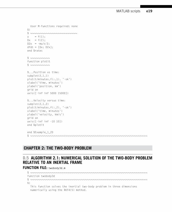
e19MATLAB scripts
User M-functions required: none
%}
% ������������������������x = f(1);
Dx = f(2);
D2x = -mu/x 2̂;
dfdt = [Dx; D2x];
end %rates
% ����������function plotit
% ����������
%...Position vs time:
subplot(2,1,1)
plot(t/minutes,f(:,1), ’-ok’)
xlabel(’time, minutes’)
ylabel(’position, km’)
grid on
axis([-inf inf 5000 15000])
%...Velocity versus time:
subplot(2,1,2)
plot(t/minutes,f(:,2), ’-ok’)
xlabel(’time, minutes’)
ylabel(’velocity, km/s’)
grid on
axis([-inf inf -10 10])
end %plotit
end %Example_1_20
% ������������������������������������������������������������
CHAPTER 2: THE TWO-BODY PROBLEM
D.5 ALGORITHM 2.1: NUMERICAL SOLUTION OF THE TWO-BODY PROBLEMRELATIVE TO AN INERTIAL FRAMEFUNCTION FILE: twobody3d.m
% ������������������������������������������������������������function twobody3d
% ������������������������������������������������������������%{
This function solves the inertial two-body problem in three dimensions
numerically using the RKF4(5) method.
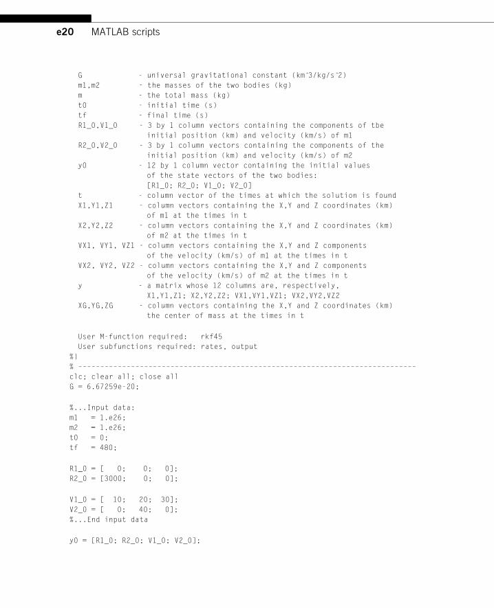
e20 MATLAB scripts
G - universal gravitational constant (km 3̂/kg/s 2̂)
m1,m2 - the masses of the two bodies (kg)
m - the total mass (kg)
t0 - initial time (s)
tf - final time (s)
R1_0,V1_0 - 3 by 1 column vectors containing the components of tbe
initial position (km) and velocity (km/s) of m1
R2_0,V2_0 - 3 by 1 column vectors containing the components of the
initial position (km) and velocity (km/s) of m2
y0 - 12 by 1 column vector containing the initial values
of the state vectors of the two bodies:
[R1_0; R2_0; V1_0; V2_0]
t - column vector of the times at which the solution is found
X1,Y1,Z1 - column vectors containing the X,Y and Z coordinates (km)
of m1 at the times in t
X2,Y2,Z2 - column vectors containing the X,Y and Z coordinates (km)
of m2 at the times in t
VX1, VY1, VZ1 - column vectors containing the X,Y and Z components
of the velocity (km/s) of m1 at the times in t
VX2, VY2, VZ2 - column vectors containing the X,Y and Z components
of the velocity (km/s) of m2 at the times in t
y - a matrix whose 12 columns are, respectively,
X1,Y1,Z1; X2,Y2,Z2; VX1,VY1,VZ1; VX2,VY2,VZ2
XG,YG,ZG - column vectors containing the X,Y and Z coordinates (km)
the center of mass at the times in t
User M-function required: rkf45
User subfunctions required: rates, output
%}
% –––––––––––––––––––––––––––––––––––––––––––––––––––––––––––––––––––––––––––––
clc; clear all; close all
G = 6.67259e-20;
%...Input data:
m1 = 1.e26;
m2 = 1.e26;
t0 = 0;
tf = 480;
R1_0 = [ 0; 0; 0];
R2_0 = [3000; 0; 0];
V1_0 = [ 10; 20; 30];
V2_0 = [ 0; 40; 0];
%...End input data
y0 = [R1_0; R2_0; V1_0; V2_0];
e21MATLAB scripts
%...Integrate the equations of motion:
[t,y] = rkf45(@rates, [t0 tf], y0);
%...Output the results:
output
return
% �������������������function dydt = rates(t,y)
% �������������������%{
This function calculates the accelerations in Equations 2.19.
t - time
y - column vector containing the position and velocity vectors
of the system at time t
R1, R2 - position vectors of m1 & m2
V1, V2 - velocity vectors of m1 & m2
r - magnitude of the relative position vector
A1, A2 - acceleration vectors of m1 & m2
dydt - column vector containing the velocity and acceleration
vectors of the system at time t
%}
% ––––––––––––––––––––––––
R1 = [y(1); y(2); y(3)];
R2 = [y(4); y(5); y(6)];
V1 = [y(7); y(8); y(9)];
V2 = [y(10); y(11); y(12)];
r = norm(R2 - R1);
A1 = G*m2*(R2 - R1)/r 3̂;
A2 = G*m1*(R1 - R2)/r 3̂;
dydt = [V1; V2; A1; A2];
end %rates
% ������������������
% ����������function output
% ����������
e22 MATLAB scripts
%{
This function calculates the trajectory of the center of mass and
plots
(a) the motion of m1, m2 and G relative to the inertial frame
(b) the motion of m2 and G relative to m1
(c) the motion of m1 and m2 relative to G
User subfunction required: common_axis_settings
%}
% –––––––––––––
%...Extract the particle trajectories:
X1 = y(:,1); Y1 = y(:,2); Z1 = y(:,3);
X2 = y(:,4); Y2 = y(:,5); Z2 = y(:,6);
%...Locate the center of mass at each time step:
XG = []; YG = []; ZG = [];
for i = 1:length(t)
XG = [XG; (m1*X1(i) + m2*X2(i))/(m1 + m2)];
YG = [YG; (m1*Y1(i) + m2*Y2(i))/(m1 + m2)];
ZG = [ZG; (m1*Z1(i) + m2*Z2(i))/(m1 + m2)];
end
%...Plot the trajectories:
figure (1)
title(’Figure 2.3: Motion relative to the inertial frame’)
hold on
plot3(X1, Y1, Z1, ’-r’)
plot3(X2, Y2, Z2, ’-g’)
plot3(XG, YG, ZG, ’-b’)
common_axis_settings
figure (2)
title(’Figure 2.4a: Motion of m2 and G relative to m1’)
hold on
plot3(X2 - X1, Y2 - Y1, Z2 - Z1, ’-g’)
plot3(XG - X1, YG - Y1, ZG - Z1, ’-b’)
common_axis_settings
figure (3)
title(’Figure 2.4b: Motion of m1 and m2 relative to G’)
hold on
plot3(X1 - XG, Y1 - YG, Z1 - ZG, ’-r’)
plot3(X2 - XG, Y2 - YG, Z2 - ZG, ’-g’)
common_axis_settings
e23MATLAB scripts
% ���������������������function common_axis_settings
% ���������������������%{
This function establishes axis properties common to the several plots.
%}
% –––––––––––––––––––––––––––
text(0, 0, 0, ’o’)
axis(’equal’)
view([2,4,1.2])
grid on
axis equal
xlabel(’X (km)’)
ylabel(’Y (km)’)
zlabel(’Z (km)’)
end %common_axis_settings
end %output
end %twobody3d
% ������������������������������������������������������������
D.6 ALGORITHM 2.2: NUMERICAL SOLUTION OF THE TWO-BODYRELATIVE MOTION PROBLEMFUNCTION FILE: orbit.m
% ������������������������������������������������������������function orbit
% ���������%{
This function computes the orbit of a spacecraft by using rkf45 to
numerically integrate Equation 2.22.
It also plots the orbit and computes the times at which the maximum
and minimum radii occur and the speeds at those times.
hours - converts hours to seconds
G - universal gravitational constant (km 3̂/kg/s 2̂)
m1 - planet mass (kg)
m2 - spacecraft mass (kg)
mu - gravitational parameter (km 3̂/s 2̂)
R - planet radius (km)
r0 - initial position vector (km)
v0 - initial velocity vector (km/s)
t0,tf - initial and final times (s)
y0 - column vector containing r0 and v0
t - column vector of the times at which the solution is found
e24 MATLAB scripts
y - a matrix whose columns are:
columns 1, 2 and 3:
The solution for the x, y and z components of the
position vector r at the times in t
columns 4, 5 and 6:
The solution for the x, y and z components of the
velocity vector v at the times in t
r - magnitude of the position vector at the times in t
imax - component of r with the largest value
rmax - largest value of r
imin - component of r with the smallest value
rmin - smallest value of r
v_at_rmax - speed where r = rmax
v_at_rmin - speed where r = rmin
User M-function required: rkf45
User subfunctions required: rates, output
%}
% –––––––––––––––––––––––––––––––––––––––––––––––––––––––––––––––––––––––––––––
clc; close all; clear all
hours = 3600;
G = 6.6742e-20;
%...Input data:
% Earth:
m1 = 5.974e24;
R = 6378;
m2 = 1000;
r0 = [8000 0 6000];
v0 = [0 7 0];
t0 = 0;
tf = 4*hours;
%...End input data
%...Numerical integration:
mu = G*(m1 + m2);
y0 = [r0 v0]’;
[t,y] = rkf45(@rates, [t0 tf], y0);
%...Output the results:
output
return
e25MATLAB scripts
% �������������������function dydt = rates(t,f)
% �������������������%{
This function calculates the acceleration vector using Equation 2.22.
t - time
f - column vector containing the position vector and the
velocity vector at time t
x, y, z - components of the position vector r
r - the magnitude of the the position vector
vx, vy, vz - components of the velocity vector v
ax, ay, az - components of the acceleration vector a
dydt - column vector containing the velocity and acceleration
components
%}
% ––––––––––––––––––––––––
x = f(1);
y = f(2);
z = f(3);
vx = f(4);
vy = f(5);
vz = f(6);
r = norm([x y z]);
ax = -mu*x/r 3̂;
ay = -mu*y/r 3̂;
az = -mu*z/r 3̂;
dydt = [vx vy vz ax ay az]’;
end %rates
% ����������function output
% ����������%{
This function computes the maximum and minimum radii, the times they
occur and and the speed at those times. It prints those results to
the command window and plots the orbit.
r - magnitude of the position vector at the times in t
imax - the component of r with the largest value
rmax - the largest value of r
imin - the component of r with the smallest value
rmin - the smallest value of r
v_at_rmax - the speed where r = rmax
v_at_rmin - the speed where r = rmin
e26 MATLAB scripts
User subfunction required: light_gray
%}
% –––––––––––––
for i = 1:length(t)
r(i) = norm([y(i,1) y(i,2) y(i,3)]);
end
[rmax imax] = max(r);
[rmin imin] = min(r);
v_at_rmax = norm([y(imax,4) y(imax,5) y(imax,6)]);
v_at_rmin = norm([y(imin,4) y(imin,5) y(imin,6)]);
%...Output to the command window:
fprintf(’\n\n––––––––––––––––––––––––––––––––––––––--–––––––––––––––––––––––
\n’)
fprintf(’\n Earth Orbit\n’)
fprintf(’ %s\n’, datestr(now))
fprintf(’\n The initial position is [%g, %g, %g] (km).’,...
r0(1), r0(2), r0(3))
fprintf(’\n Magnitude = %g km\n’, norm(r0))
fprintf(’\n The initial velocity is [%g, %g, %g] (km/s).’,...
v0(1), v0(2), v0(3))
fprintf(’\n Magnitude = %g km/s\n’, norm(v0))
fprintf(’\n Initial time = %g h.\n Final time = %g h.\n’,0,tf/hours)
fprintf(’\n The minimum altitude is %g km at time = %g h.’,...
rmin-R, t(imin)/hours)
fprintf(’\n The speed at that point is %g km/s.\n’, v_at_rmin)
fprintf(’\n The maximum altitude is %g km at time = %g h.’,...
rmax-R, t(imax)/hours)
fprintf(’\n The speed at that point is %g km/s\n’, v_at_rmax)
fprintf(’\n––––––––––––––––––––––––––––––––––––––––––––––––––––––––––––––\n\n’)
%...Plot the results:
% Draw the planet
[xx, yy, zz] = sphere(100);
surf(R*xx, R*yy, R*zz)
colormap(light_gray)
caxis([-R/100 R/100])
shading interp
% Draw and label the X, Y and Z axes
line([0 2*R], [0 0], [0 0]); text(2*R, 0, 0, ’X’)
line( [0 0], [0 2*R], [0 0]); text( 0, 2*R, 0, ’Y’)
line( [0 0], [0 0], [0 2*R]); text( 0, 0, 2*R, ’Z’)
e27MATLAB scripts
% Plot the orbit, draw a radial to the starting point
% and label the starting point (o) and the final point (f)
hold on
plot3( y(:,1), y(:,2), y(:,3),’k’)
line([0 r0(1)], [0 r0(2)], [0 r0(3)])
text( y(1,1), y(1,2), y(1,3), ’o’)
text( y(end,1), y(end,2), y(end,3), ’f’)
% Select a view direction (a vector directed outward from the origin)
view([1,1,.4])
% Specify some properties of the graph
grid on
axis equal
xlabel(’km’)
ylabel(’km’)
zlabel(’km’)
% ������������������function map = light_gray
% ������������������%{
This function creates a color map for displaying the planet as light
gray with a black equator.
r - fraction of red
g - fraction of green
b - fraction of blue
%}
% –––––––––––––––––––––––
r = 0.8; g = r; b = r;
map = [r g b
0 0 0
r g b];
end %light_gray
end %output
end %orbit
% ������������������������������������������������������������
e28 MATLAB scripts
D.7 CALCULATION OF THE LAGRANGE F AND G FUNCTIONS AND THEIR TIMEDERIVATIVES IN TERMS OF CHANGE IN TRUE ANOMALYFUNCTION FILE: f_and_g_ta.m
% �����������������������������������function [f, g] = f_and_g_ta(r0, v0, dt, mu)
% �����������������������������������%{
This function calculates the Lagrange f and g coefficients from the
change in true anomaly since time t0.
mu - gravitational parameter (km 3̂/s 2̂)
dt - change in true anomaly (degrees)
r0 - position vector at time t0 (km)
v0 - velocity vector at time t0 (km/s)
h - angular momentum (km 2̂/s)
vr0 - radial component of v0 (km/s)
r - radial position after the change in true anomaly
f - the Lagrange f coefficient (dimensionless)
g - the Lagrange g coefficient (s)
User M-functions required: None
%}
% ––––––––––––––––––––––––––––––––––––––––––––
h = norm(cross(r0,v0));
vr0 = dot(v0,r0)/norm(r0);
r0 = norm(r0);
s = sind(dt);
c = cosd(dt);
%...Equation 2.152:
r = h 2̂/mu/(1 + (h 2̂/mu/r0 - 1)*c - h*vr0*s/mu);
%...Equations 2.158a & b:
f = 1 - mu*r*(1 - c)/h 2̂;
g = r*r0*s/h;
end
% ���������������������������������
FUNCTION FILE: fDot_and_gDot_ta.m
% ���������������������������������������������function [fdot, gdot] = fDot_and_gDot_ta(r0, v0, dt, mu)
% ���������������������������������������������
e29MATLAB scripts
%{
This function calculates the time derivatives of the Lagrange
f and g coefficients from the change in true anomaly since time t0.
mu - gravitational parameter (km 3̂/s 2̂)
dt - change in true anomaly (degrees)
r0 - position vector at time t0 (km)
v0 - velocity vector at time t0 (km/s)
h - angular momentum (km 2̂/s)
vr0 - radial component of v0 (km/s)
fdot - time derivative of the Lagrange f coefficient (1/s)
gdot - time derivative of the Lagrange g coefficient (dimensionless)
User M-functions required: None
%}
% ––––––––––––––––––––––––––––––––––––––––––––––––––––––––
h = norm(cross(r0,v0));
vr0 = dot(v0,r0)/norm(r0);
r0 = norm(r0);
c = cosd(dt);
s = sind(dt);
%...Equations 2.158c & d:
fdot = mu/h*(vr0/h*(1 - c) - s/r0);
gdot = 1 - mu*r0/h 2̂*(1 - c);
end
% ���������������������������������������������
D.8 ALGORITHM 2.3: CALCULATE THE STATE VECTOR FROM THE INITIALSTATE VECTOR AND THE CHANGE IN TRUE ANOMALYFUNCTION FILE: rv_from_r0v0_ta.m
% ��������������������������������������function [r,v] = rv_from_r0v0_ta(r0, v0, dt, mu)
% ��������������������������������������%{
This function computes the state vector (r,v) from the
initial state vector (r0,v0) and the change in true anomaly.
mu - gravitational parameter (km 3̂/s 2̂)
r0 - initial position vector (km)
v0 - initial velocity vector (km/s)
e30 MATLAB scripts
dt - change in true anomaly (degrees)
r - final position vector (km)
v - final velocity vector (km/s)
User M-functions required: f_and_g_ta, fDot_and_gDot_ta
%}
% –––––––––––––––––––––––––––––––––––––––––––––––––––––––––––––––––––––––––––––
%global mu
%...Compute the f and g functions and their derivatives:
[f, g] = f_and_g_ta(r0, v0, dt, mu);
[fdot, gdot] = fDot_and_gDot_ta(r0, v0, dt, mu);
%...Compute the final position and velocity vectors:
r = f*r0 +g*v0;
v = fdot*r0 + gdot*v0;
end
% �������������������������������������
SCRIPT FILE: Example_2_13.m
% ���������������������������������������% Example_2_13
% ����������%{
This program computes the state vector [R,V] from the initial
state vector [R0,V0] and the change in true anomaly, using the
data in Example 2.13
mu - gravitational parameter (km 3̂/s 2̂)
R0 - the initial position vector (km)
V0 - the initial velocity vector (km/s)
r0 - magnitude of R0
v0 - magnitude of V0
R - final position vector (km)
V - final velocity vector (km/s)
r - magnitude of R
v - magnitude of V
dt - change in true anomaly (degrees)
User M-functions required: rv_from_r0v0_ta
%}
% ––––––––––––––––––––––––––––––––––––––––––––––––––
e31MATLAB scripts
clear all; clc
mu = 398600;
%...Input data:
R0 = [8182.4 -6865.9 0];
V0 = [0.47572 8.8116 0];
dt = 120;
%...End input data
%...Algorithm 2.3:
[R,V] = rv_from_r0v0_ta(R0, V0, dt, mu);
r = norm(R);
v = norm(V);
r0 = norm(R0);
v0 = norm(V0);
fprintf(’––––––––––––––––––––––––––––––––––––––––––––––––––––––––––––––––––––’)
fprintf(’\n Example 2.13 \n’)
fprintf(’\n Initial state vector:\n’)
fprintf(’\n r = [%g, %g, %g] (km)’, R0(1), R0(2), R0(3))
fprintf(’\n magnitude = %g\n’, norm(R0))
fprintf(’\n v = [%g, %g, %g] (km/s)’, V0(1), V0(2), V0(3))
fprintf(’\n magnitude = %g’, norm(V0))
fprintf(’\n\n State vector after %g degree change in true anomaly:\n’, dt)
fprintf(’\n r = [%g, %g, %g] (km)’, R(1), R(2), R(3))
fprintf(’\n magnitude = %g\n’, norm(R))
fprintf(’\n v = [%g, %g, %g] (km/s)’, V(1), V(2), V(3))
fprintf(’\n magnitude = %g’, norm(V))
fprintf(’\n––––––––––––––––––––––––––––––––––––––––––––––––––––––––––––––––\n’)
% ���������������������������������������
OUTPUT FROM Example_2_13.m
–––––––––––––––––––––––––––––––––––––––––––––––––––––––––––
Example 2.13
Initial state vector:
r = [8182.4, -6865.9, 0] (km)
magnitude = 10681.4
v = [0.47572, 8.8116, 0] (km/s)
magnitude = 8.82443
e32 MATLAB scripts
State vector after 120 degree change in true anomaly:
r = [1454.99, 8251.47, 0] (km)
magnitude = 8378.77
v = [-8.13238, 5.67854, -0] (km/s)
magnitude = 9.91874
–––––––––––––––––––––––––––––––––––––––––––––––––––––––––––
D.9 ALGORITHM 2.4: FIND THE ROOT OF A FUNCTION USING THEBISECTION METHODFUNCTION FILE: bisect.m
% ����������������������������������������������function root = bisect(fun, xl, xu)
% ��������������������������%{
This function evaluates a root of a function using
the bisection method.
tol - error to within which the root is computed
n - number of iterations
xl - low end of the interval containing the root
xu - upper end of the interval containing the root
i - loop index
xm - mid-point of the interval from xl to xu
fun - name of the function whose root is being found
fxl - value of fun at xl
fxm - value of fun at xm
root - the computed root
User M-functions required: none
%}
% ––––––––––––––––––––––––––––––––––––––––––––––
tol = 1.e-6;
n = ceil(log(abs(xu - xl)/tol)/log(2));
for i = 1:n
xm = (xl + xu)/2;
fxl = feval(fun, xl);
fxm = feval(fun, xm);
if fxl*fxm > 0
xl = xm;
else
xu = xm;
end
end
e33MATLAB scripts
root = xm;
end
% �����������������������������������
FUNCTION FILE: Example_2_16.m
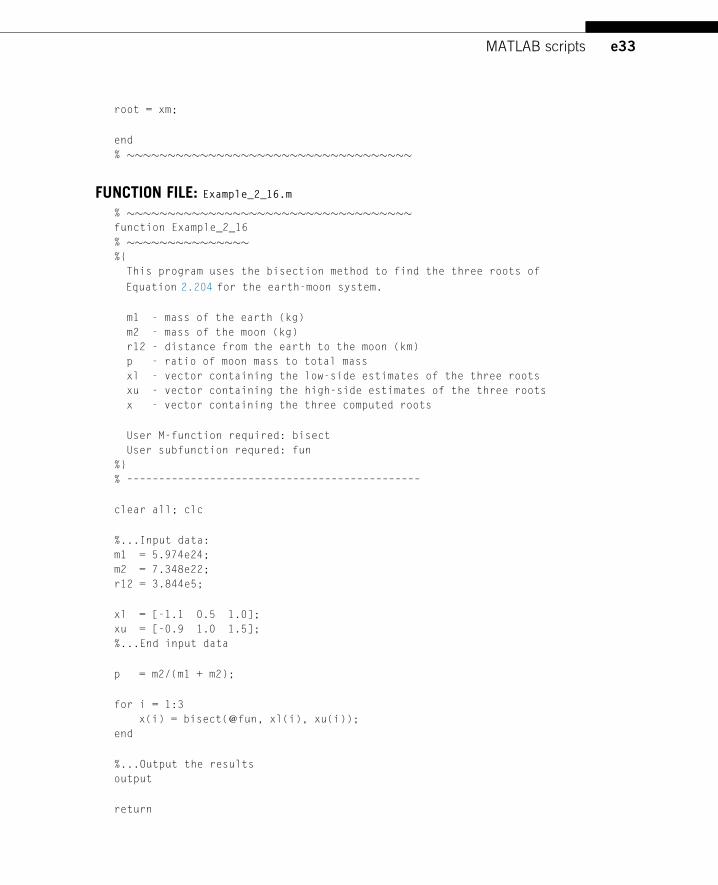
% �����������������������������������function Example_2_16
% ���������������%{
This program uses the bisection method to find the three roots of
Equation 2.204 for the earth-moon system.
m1 - mass of the earth (kg)
m2 - mass of the moon (kg)
r12 - distance from the earth to the moon (km)
p - ratio of moon mass to total mass
xl - vector containing the low-side estimates of the three roots
xu - vector containing the high-side estimates of the three roots
x - vector containing the three computed roots
User M-function required: bisect
User subfunction requred: fun
%}
% ––––––––––––––––––––––––––––––––––––––––––––––
clear all; clc
%...Input data:
m1 = 5.974e24;
m2 = 7.348e22;
r12 = 3.844e5;
xl = [-1.1 0.5 1.0];
xu = [-0.9 1.0 1.5];
%...End input data
p = m2/(m1 + m2);
for i = 1:3
x(i) = bisect(@fun, xl(i), xu(i));
end
%...Output the results
output
return
e34 MATLAB scripts
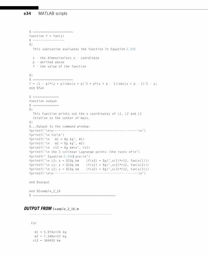
% �����������������function f = fun(z)
% –––––––––––––––––
%{
This subroutine evaluates the function in Equation 2.204
z - the dimensionless x - coordinate
p - defined above
f - the value of the function
%}
% �����������������f = (1 - p)*(z + p)/abs(z + p) 3̂ + p*(z + p - 1)/abs(z + p - 1) 3̂ - z;
end %fun
% �����������function output
% �����������%{
This function prints out the x coordinates of L1, L2 and L3
relative to the center of mass.
%}
%...Output to the command window:
fprintf(’\n\n––––––––––––––––––––––––––––––––––––––--––––––\n’)
fprintf(’\n For\n’)
fprintf(’\n m1 = %g kg’, m1)
fprintf(’\n m2 = %g kg’, m2)
fprintf(’\n r12 = %g km\n’, r12)
fprintf(’\n the 3 colinear Lagrange points (the roots of\n’)
fprintf(’ Equation 2.204) are:\n’)
fprintf(’\n L3: x = %10g km (f(x3) = %g)’,x(1)*r12, fun(x(1)))
fprintf(’\n L1: x = %10g km (f(x1) = %g)’,x(2)*r12, fun(x(2)))
fprintf(’\n L2: x = %10g km (f(x2) = %g)’,x(3)*r12, fun(x(3)))
fprintf(’\n\n––––––––––––––––––––––––––––––––––––––--––––––\n’)
end %output
end %Example_2_16
% �����������������������������������
OUTPUT FROM Example_2_16.m
–––––––––––––––––––––––––––––––––––––––––––––
For
m1 = 5.974e+24 kg
m2 = 7.348e+22 kg
r12 = 384400 km
e35MATLAB scripts
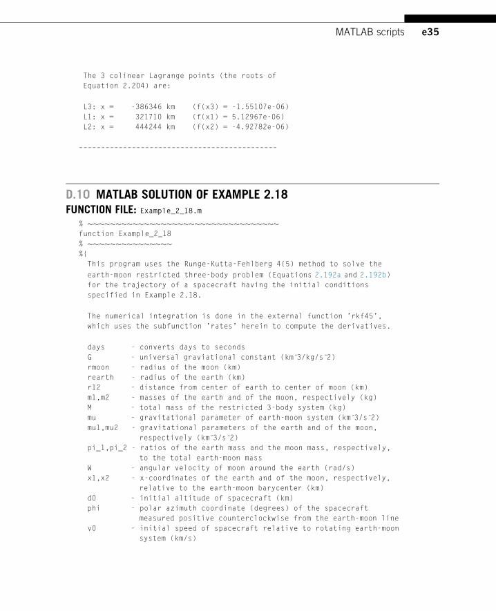
The 3 colinear Lagrange points (the roots of
Equation 2.204) are:
L3: x = -386346 km (f(x3) = -1.55107e-06)
L1: x = 321710 km (f(x1) = 5.12967e-06)
L2: x = 444244 km (f(x2) = -4.92782e-06)
–––––––––––––––––––––––––––––––––––––––––––––
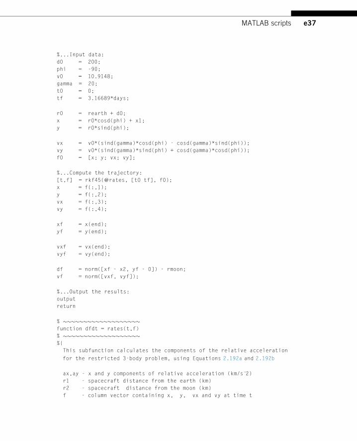
D.10 MATLAB SOLUTION OF EXAMPLE 2.18FUNCTION FILE: Example_2_18.m
% ����������������������������������function Example_2_18
% ���������������%{
This program uses the Runge-Kutta-Fehlberg 4(5) method to solve the
earth-moon restricted three-body problem (Equations 2.192a and 2.192b)
for the trajectory of a spacecraft having the initial conditions
specified in Example 2.18.
The numerical integration is done in the external function ’rkf45’,
which uses the subfunction ’rates’ herein to compute the derivatives.
days - converts days to seconds
G - universal graviational constant (km 3̂/kg/s 2̂)
rmoon - radius of the moon (km)
rearth - radius of the earth (km)
r12 - distance from center of earth to center of moon (km)
m1,m2 - masses of the earth and of the moon, respectively (kg)
M - total mass of the restricted 3-body system (kg)
mu - gravitational parameter of earth-moon system (km 3̂/s 2̂)
mu1,mu2 - gravitational parameters of the earth and of the moon,
respectively (km 3̂/s 2̂)
pi_1,pi_2 - ratios of the earth mass and the moon mass, respectively,
to the total earth-moon mass
W - angular velocity of moon around the earth (rad/s)
x1,x2 - x-coordinates of the earth and of the moon, respectively,
relative to the earth-moon barycenter (km)
d0 - initial altitude of spacecraft (km)
phi - polar azimuth coordinate (degrees) of the spacecraft
measured positive counterclockwise from the earth-moon line
v0 - initial speed of spacecraft relative to rotating earth-moon
system (km/s)
e36 MATLAB scripts
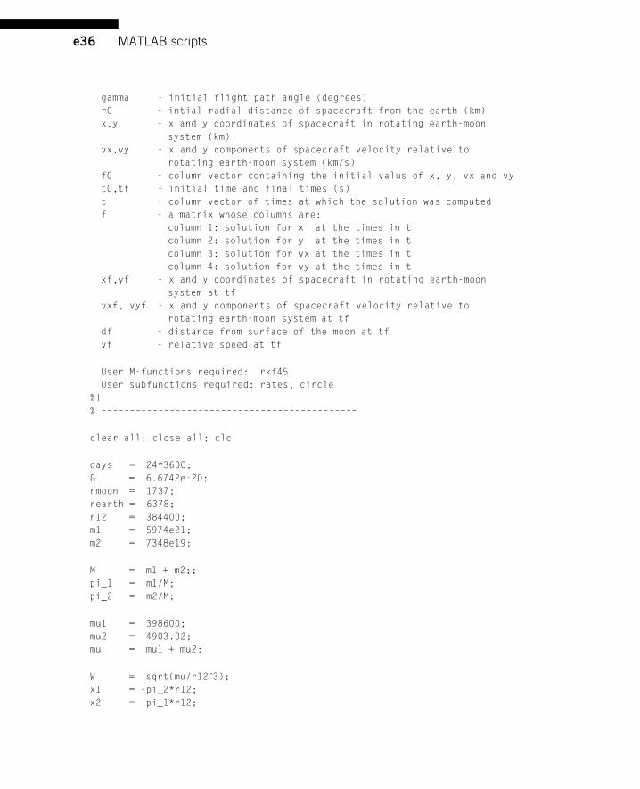
gamma - initial flight path angle (degrees)
r0 - intial radial distance of spacecraft from the earth (km)
x,y - x and y coordinates of spacecraft in rotating earth-moon
system (km)
vx,vy - x and y components of spacecraft velocity relative to
rotating earth-moon system (km/s)
f0 - column vector containing the initial valus of x, y, vx and vy
t0,tf - initial time and final times (s)
t - column vector of times at which the solution was computed
f - a matrix whose columns are:
column 1: solution for x at the times in t
column 2: solution for y at the times in t
column 3: solution for vx at the times in t
column 4: solution for vy at the times in t
xf,yf - x and y coordinates of spacecraft in rotating earth-moon
system at tf
vxf, vyf - x and y components of spacecraft velocity relative to
rotating earth-moon system at tf
df - distance from surface of the moon at tf
vf - relative speed at tf
User M-functions required: rkf45
User subfunctions required: rates, circle
%}
% –––––––––––––––––––––––––––––––––––––––––––––
clear all; close all; clc
days = 24*3600;
G = 6.6742e-20;
rmoon = 1737;
rearth = 6378;
r12 = 384400;
m1 = 5974e21;
m2 = 7348e19;
M = m1 + m2;;
pi_1 = m1/M;
pi_2 = m2/M;
mu1 = 398600;
mu2 = 4903.02;
mu = mu1 + mu2;
W = sqrt(mu/r12 3̂);
x1 = -pi_2*r12;
x2 = pi_1*r12;
e37MATLAB scripts
%...Input data:
d0 = 200;
phi = -90;
v0 = 10.9148;
gamma = 20;
t0 = 0;
tf = 3.16689*days;
r0 = rearth + d0;
x = r0*cosd(phi) + x1;
y = r0*sind(phi);
vx = v0*(sind(gamma)*cosd(phi) - cosd(gamma)*sind(phi));
vy = v0*(sind(gamma)*sind(phi) + cosd(gamma)*cosd(phi));
f0 = [x; y; vx; vy];
%...Compute the trajectory:
[t,f] = rkf45(@rates, [t0 tf], f0);
x = f(:,1);
y = f(:,2);
vx = f(:,3);
vy = f(:,4);
xf = x(end);
yf = y(end);
vxf = vx(end);
vyf = vy(end);
df = norm([xf - x2, yf - 0]) - rmoon;
vf = norm([vxf, vyf]);
%...Output the results:
output
return
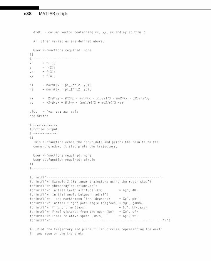
% �������������������function dfdt = rates(t,f)
% �������������������%{
This subfunction calculates the components of the relative acceleration
for the restricted 3-body problem, using Equations 2.192a and 2.192b
ax,ay - x and y components of relative acceleration (km/s 2̂)
r1 - spacecraft distance from the earth (km)
r2 - spacecraft distance from the moon (km)
f - column vector containing x, y, vx and vy at time t
e38 MATLAB scripts
dfdt - column vector containing vx, vy, ax and ay at time t
All other variables are defined above.
User M-functions required: none
%}
% ––––––––––––––––––––––––
x = f(1);
y = f(2);
vx = f(3);
vy = f(4);
r1 = norm([x + pi_2*r12, y]);
r2 = norm([x - pi_1*r12, y]);
ax = 2*W*vy + W 2̂*x - mu1*(x - x1)/r1 3̂ - mu2*(x - x2)/r2 3̂;
ay = -2*W*vx + W 2̂*y - (mu1/r1 3̂ + mu2/r2 3̂)*y;
dfdt = [vx; vy; ax; ay];
end %rates
% ����������function output
% ����������%{
This subfunction echos the input data and prints the results to the
command window. It also plots the trajectory.
User M-functions required: none
User subfunction required: circle
%}
% –––––––––––––
fprintf(’––––––––––––––––––––––––––––––––––––––––––––––––––––––––––––’)
fprintf(’\n Example 2.18: Lunar trajectory using the restricted’)
fprintf(’\n threebody equations.\n’)
fprintf(’\n Initial Earth altitude (km) = %g’, d0)
fprintf(’\n Initial angle between radial’)
fprintf(’\n and earth-moon line (degrees) = %g’, phi)
fprintf(’\n Initial flight path angle (degrees) = %g’, gamma)
fprintf(’\n Flight time (days) = %g’, tf/days)
fprintf(’\n Final distance from the moon (km) = %g’, df)
fprintf(’\n Final relative speed (km/s) = %g’, vf)
fprintf(’\n––––––––––––––––––––––––––––––––––––––––––––––––––––––––––––\n’)
%...Plot the trajectory and place filled circles representing the earth
% and moon on the the plot:
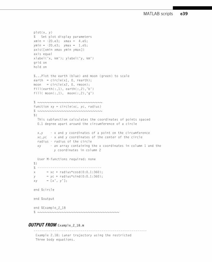
e39MATLAB scripts
plot(x, y)
% Set plot display parameters
xmin = -20.e3; xmax = 4.e5;
ymin = -20.e3; ymax = 1.e5;
axis([xmin xmax ymin ymax])
axis equal
xlabel(’x, km’); ylabel(’y, km’)
grid on
hold on
%...Plot the earth (blue) and moon (green) to scale
earth = circle(x1, 0, rearth);
moon = circle(x2, 0, rmoon);
fill(earth(:,1), earth(:,2),’b’)
fill( moon(:,1), moon(:,2),’g’)
% ���������������������������function xy = circle(xc, yc, radius)
% ���������������������������%{
This subfunction calculates the coordinates of points spaced
0.1 degree apart around the circumference of a circle
x,y - x and y coordinates of a point on the circumference
xc,yc - x and y coordinates of the center of the circle
radius - radius of the circle
xy - an array containing the x coordinates in column 1 and the
y coordinates in column 2
User M-functions required: none
%}
% ––––––––––––––––––––––––––––––––––
x = xc + radius*cosd(0:0.1:360);
y = yc + radius*sind(0:0.1:360);
xy = [x’, y’];
end %circle
end %output
end %Example_2_18
% ����������������������������������
OUTPUT FROM Example_2_18.m
––––––––––––––––––––––––––––––––––––––––––––––––––––––––––––
Example 2.18: Lunar trajectory using the restricted
Three body equations.
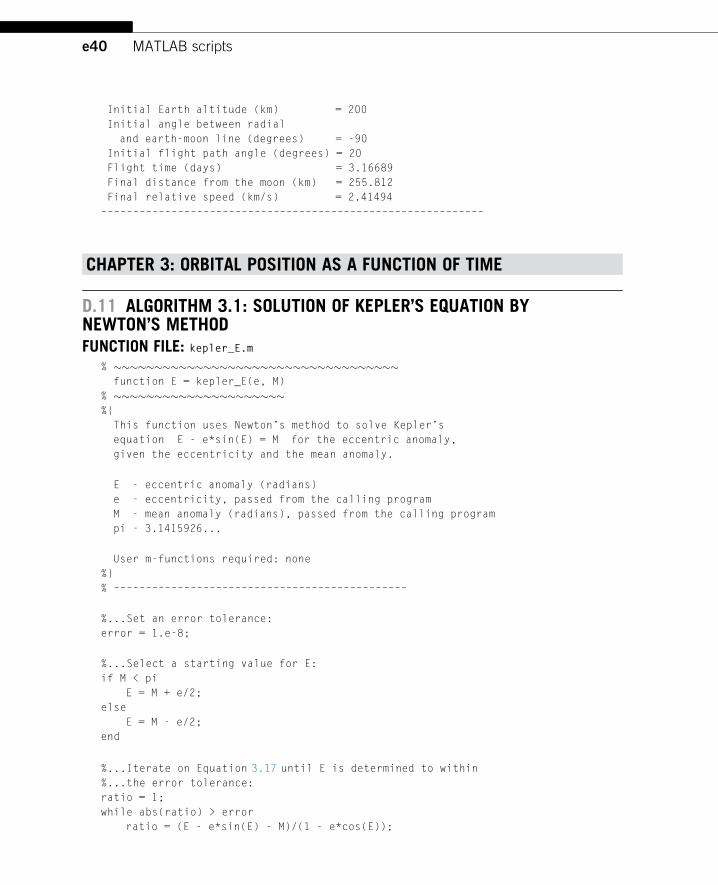
e40 MATLAB scripts
Initial Earth altitude (km) = 200
Initial angle between radial
and earth-moon line (degrees) = -90
Initial flight path angle (degrees) = 20
Flight time (days) = 3.16689
Final distance from the moon (km) = 255.812
Final relative speed (km/s) = 2.41494
––––––––––––––––––––––––––––––––––––––––––––––––––––––––––––
CHAPTER 3: ORBITAL POSITION AS A FUNCTION OF TIME
D.11 ALGORITHM 3.1: SOLUTION OF KEPLER’S EQUATION BYNEWTON’S METHODFUNCTION FILE: kepler_E.m
% �����������������������������������function E = kepler_E(e, M)
% ���������������������%{
This function uses Newton’s method to solve Kepler’s
equation E - e*sin(E) = M for the eccentric anomaly,
given the eccentricity and the mean anomaly.
E - eccentric anomaly (radians)
e - eccentricity, passed from the calling program
M - mean anomaly (radians), passed from the calling program
pi - 3.1415926...
User m-functions required: none
%}
% ––––––––––––––––––––––––––––––––––––––––––––––
%...Set an error tolerance:
error = 1.e-8;
%...Select a starting value for E:
if M < pi
E = M + e/2;
else
E = M - e/2;
end
%...Iterate on Equation 3.17 until E is determined to within
%...the error tolerance:
ratio = 1;
while abs(ratio) > error
ratio = (E - e*sin(E) - M)/(1 - e*cos(E));
e41MATLAB scripts
E = E - ratio;
end
end %kepler_E
% �����������������������������������
SCRIPT FILE: Example_3_02.m
% �����������������������������������% Example_3_02
% ����������%{
This program uses Algorithm 3.1 and the data of Example 3.2 to solve
Kepler’s equation.
e - eccentricity
M - mean anomaly (rad)
E - eccentric anomaly (rad)
User M-function required: kepler_E
%}
% ––––––––––––––––––––––––––––––––––––––––––––––
clear all; clc
%...Data declaration for Example 3.2:
e = 0.37255;
M = 3.6029;
%...
%...Pass the input data to the function kepler_E, which returns E:
E = kepler_E(e, M);
%...Echo the input data and output to the command window:
fprintf(’–––––––––––––––––––––––––––––––––––––––––––––––––––––’)
fprintf(’\n Example 3.2\n’)
fprintf(’\n Eccentricity = %g’,e)
fprintf(’\n Mean anomaly (radians) = %g\n’,M)
fprintf(’\n Eccentric anomaly (radians) = %g’,E)
fprintf(’\n–––––––––––––––––––––––––––––––––––––––––––––––––––––\n’)
% �����������������������������������
OUTPUT FROM Example_3_02.m
–––––––––––––––––––––––––––––––––––––––––––––––––––––
Example 3.2
Eccentricity = 0.37255
Mean anomaly (radians) = 3.6029
e42 MATLAB scripts
Eccentric anomaly (radians) = 3.47942
–––––––––––––––––––––––––––––––––––––––––––––––––––––
D.12 ALGORITHM 3.2: SOLUTION OF KEPLER’S EQUATION FOR THEHYPERBOLA USING NEWTON’S METHODFUNCTION FILE: kepler_H.m
% �����������������������������������function F = kepler_H(e, M)
% ���������������������%{
This function uses Newton’s method to solve Kepler’s equation
for the hyperbola e*sinh(F) - F = M for the hyperbolic
eccentric anomaly, given the eccentricity and the hyperbolic
mean anomaly.
F - hyperbolic eccentric anomaly (radians)
e - eccentricity, passed from the calling program
M - hyperbolic mean anomaly (radians), passed from the
calling program
User M-functions required: none
%}
% ––––––––––––––––––––––––––––––––––––––––––––––
%...Set an error tolerance:
error = 1.e-8;
%...Starting value for F:
F = M;
%...Iterate on Equation 3.45 until F is determined to within
%...the error tolerance:
ratio = 1;
while abs(ratio) > error
ratio = (e*sinh(F) - F - M)/(e*cosh(F) - 1);
F = F - ratio;
end
end %kepler_H
% �����������������������������������
e43MATLAB scripts
SCRIPT FILE: Example_3_05.m
% �����������������������������������% Example_3_05
% ���������%{
This program uses Algorithm 3.2 and the data of
Example 3.5 to solve Kepler’s equation for the hyperbola.
e - eccentricity
M - hyperbolic mean anomaly (dimensionless)
F - hyperbolic eccentric anomaly (dimensionless)
User M-function required: kepler_H
%}
% ––––––––––––––––––––––––––––––––––––––––––––––
clear
%...Data declaration for Example 3.5:
e = 2.7696;
M = 40.69;
%...
%...Pass the input data to the function kepler_H, which returns F:
F = kepler_H(e, M);
%...Echo the input data and output to the command window:
fprintf(’–––––––––––––––––––––––––––––––––––––––––––––––––––––’)
fprintf(’\n Example 3.5\n’)
fprintf(’\n Eccentricity = %g’,e)
fprintf(’\n Hyperbolic mean anomaly = %g\n’,M)
fprintf(’\n Hyperbolic eccentric anomaly = %g’,F)
fprintf(’\n–––––––––––––––––––––––––––––––––––––––––––––––––––––\n’)
% �����������������������������������
OUTPUT FROM Example_3_05.m
–––––––––––––––––––––––––––––––––––––––––––––––––––––
Example 3.5
Eccentricity = 2.7696
Hyperbolic mean anomaly = 40.69
Hyperbolic eccentric anomaly = 3.46309
–––––––––––––––––––––––––––––––––––––––––––––––––––––
e44 MATLAB scripts
D.13 CALCULATION OF THE STUMPFF FUNCTIONS S(Z) AND C(Z)The following scripts implement Eqs. (3.52) and (3.53) for use in other programs.
FUNCTION FILE: stumpS.m
% �����������������������������������function s = stumpS(z)
% �����������������%{
This function evaluates the Stumpff function S(z) according
to Equation 3.52.
z - input argument
s - value of S(z)
User M-functions required: none
%}
% ––––––––––––––––––––––––––––––––––––––––––––––
if z > 0
s = (sqrt(z) - sin(sqrt(z)))/(sqrt(z)) 3̂;
elseif z < 0
s = (sinh(sqrt(-z)) - sqrt(-z))/(sqrt(-z)) 3̂;
else
s = 1/6;
end
% �����������������������������������
FUNCTION FILE: stumpC.m
% �����������������������������������function c = stumpC(z)
% �����������������%{
This function evaluates the Stumpff function C(z) according
to Equation 3.53.
z - input argument
c - value of C(z)
User M-functions required: none
%}
% ––––––––––––––––––––––––––––––––––––––––––––––
if z > 0
c = (1 - cos(sqrt(z)))/z;
elseif z < 0
c = (cosh(sqrt(-z)) - 1)/(-z);
e45MATLAB scripts
else
c = 1/2;
end
% �����������������������������������
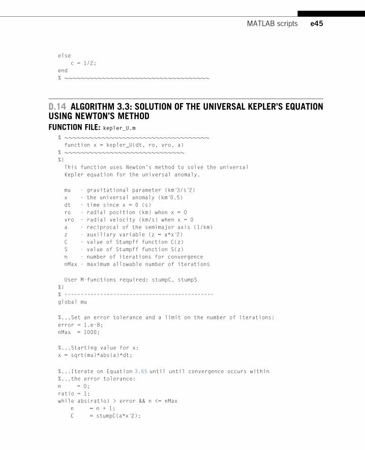
D.14 ALGORITHM 3.3: SOLUTION OF THE UNIVERSAL KEPLER’S EQUATIONUSING NEWTON’S METHODFUNCTION FILE: kepler_U.m
% �����������������������������������function x = kepler_U(dt, ro, vro, a)
% �����������������������������%{
This function uses Newton’s method to solve the universal
Kepler equation for the universal anomaly.
mu - gravitational parameter (km 3̂/s 2̂)
x - the universal anomaly (km 0̂.5)
dt - time since x = 0 (s)
ro - radial position (km) when x = 0
vro - radial velocity (km/s) when x = 0
a - reciprocal of the semimajor axis (1/km)
z - auxiliary variable (z = a*x 2̂)
C - value of Stumpff function C(z)
S - value of Stumpff function S(z)
n - number of iterations for convergence
nMax - maximum allowable number of iterations
User M-functions required: stumpC, stumpS
%}
% ––––––––––––––––––––––––––––––––––––––––––––––
global mu
%...Set an error tolerance and a limit on the number of iterations:
error = 1.e-8;
nMax = 1000;
%...Starting value for x:
x = sqrt(mu)*abs(a)*dt;
%...Iterate on Equation 3.65 until until convergence occurs within
%...the error tolerance:
n = 0;
ratio = 1;
while abs(ratio) > error && n <= nMax
n = n + 1;
C = stumpC(a*x 2̂);
e46 MATLAB scripts
S = stumpS(a*x 2̂);
F = ro*vro/sqrt(mu)*x 2̂*C + (1 - a*ro)*x 3̂*S + ro*x - sqrt(mu)*dt;
dFdx = ro*vro/sqrt(mu)*x*(1 - a*x 2̂*S) + (1 - a*ro)*x 2̂*C + ro;
ratio = F/dFdx;
x = x - ratio;
end
%...Deliver a value for x, but report that nMax was reached:
if n > nMax
fprintf(’\n **No. iterations of Kepler’s equation = %g’, n)
fprintf(’\n F/dFdx = %g\n’, F/dFdx)
end
% �����������������������������������
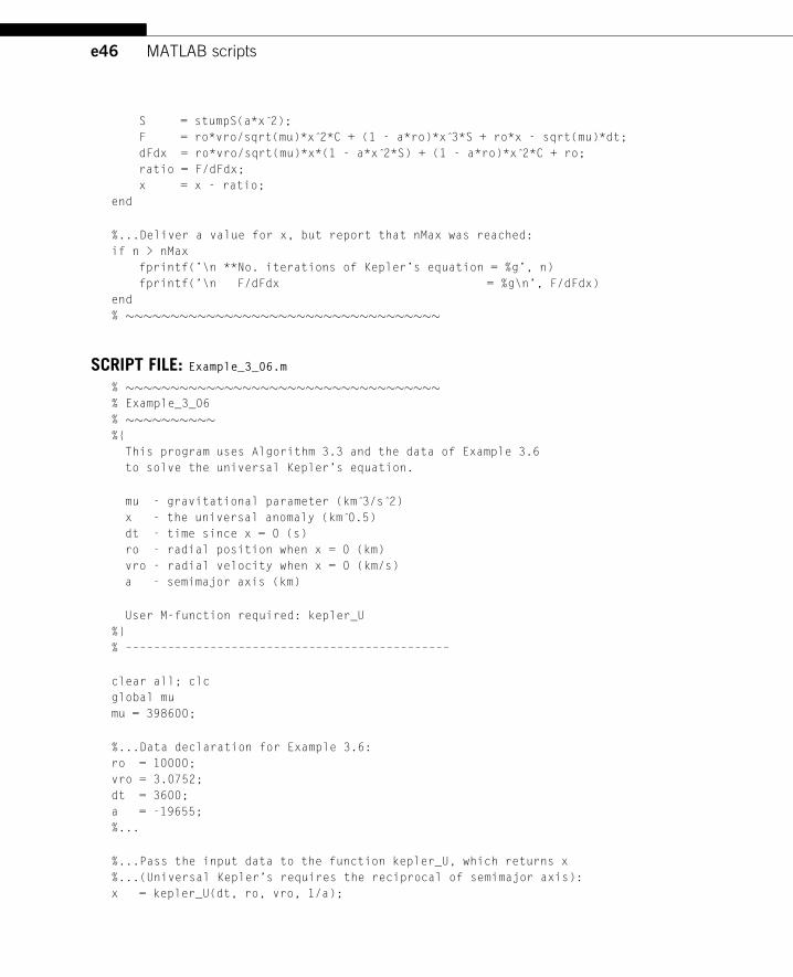
SCRIPT FILE: Example_3_06.m
% �����������������������������������% Example_3_06
% ����������%{
This program uses Algorithm 3.3 and the data of Example 3.6
to solve the universal Kepler’s equation.
mu - gravitational parameter (km 3̂/s 2̂)
x - the universal anomaly (km 0̂.5)
dt - time since x = 0 (s)
ro - radial position when x = 0 (km)
vro - radial velocity when x = 0 (km/s)
a - semimajor axis (km)
User M-function required: kepler_U
%}
% ––––––––––––––––––––––––––––––––––––––––––––––
clear all; clc
global mu
mu = 398600;
%...Data declaration for Example 3.6:
ro = 10000;
vro = 3.0752;
dt = 3600;
a = -19655;
%...
%...Pass the input data to the function kepler_U, which returns x
%...(Universal Kepler’s requires the reciprocal of semimajor axis):
x = kepler_U(dt, ro, vro, 1/a);
e47MATLAB scripts
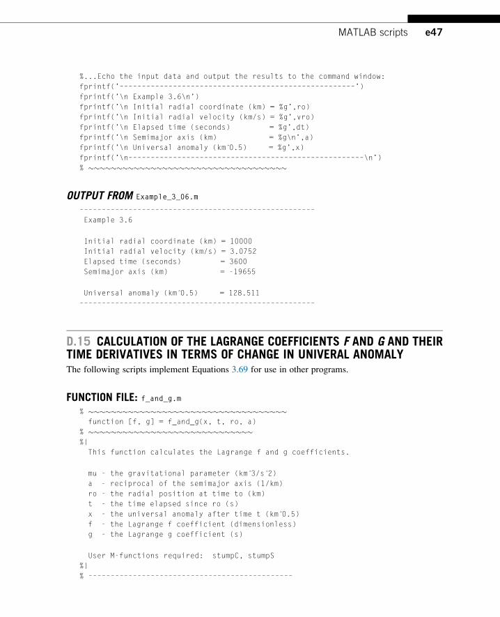
%...Echo the input data and output the results to the command window:
fprintf(’–––––––––––––––––––––––––––––––––––––––––––––––––––––’)
fprintf(’\n Example 3.6\n’)
fprintf(’\n Initial radial coordinate (km) = %g’,ro)
fprintf(’\n Initial radial velocity (km/s) = %g’,vro)
fprintf(’\n Elapsed time (seconds) = %g’,dt)
fprintf(’\n Semimajor axis (km) = %g\n’,a)
fprintf(’\n Universal anomaly (km 0̂.5) = %g’,x)
fprintf(’\n–––––––––––––––––––––––––––––––––––––––––––––––––––––\n’)
% �����������������������������������
OUTPUT FROM Example_3_06.m
–––––––––––––––––––––––––––––––––––––––––––––––––––––
Example 3.6
Initial radial coordinate (km) = 10000
Initial radial velocity (km/s) = 3.0752
Elapsed time (seconds) = 3600
Semimajor axis (km) = -19655
Universal anomaly (km 0̂.5) = 128.511
–––––––––––––––––––––––––––––––––––––––––––––––––––––
D.15 CALCULATION OF THE LAGRANGE COEFFICIENTS F AND G AND THEIRTIME DERIVATIVES IN TERMS OF CHANGE IN UNIVERAL ANOMALYThe following scripts implement Equations 3.69 for use in other programs.
FUNCTION FILE: f_and_g.m
% �����������������������������������function [f, g] = f_and_g(x, t, ro, a)
% �����������������������������%{
This function calculates the Lagrange f and g coefficients.
mu - the gravitational parameter (km 3̂/s 2̂)
a - reciprocal of the semimajor axis (1/km)
ro - the radial position at time to (km)
t - the time elapsed since ro (s)
x - the universal anomaly after time t (km 0̂.5)
f - the Lagrange f coefficient (dimensionless)
g - the Lagrange g coefficient (s)
User M-functions required: stumpC, stumpS
%}
% ––––––––––––––––––––––––––––––––––––––––––––––
e48 MATLAB scripts
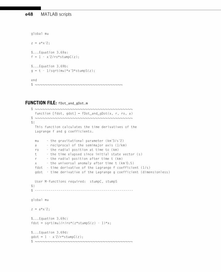
global mu
z = a*x 2̂;
%...Equation 3.69a:
f = 1 - x 2̂/ro*stumpC(z);
%...Equation 3.69b:
g = t - 1/sqrt(mu)*x 3̂*stumpS(z);
end
% �����������������������������������
FUNCTION FILE: fDot_and_gDot.m
% ���������������������������������������function [fdot, gdot] = fDot_and_gDot(x, r, ro, a)
% ���������������������������������������%{
This function calculates the time derivatives of the
Lagrange f and g coefficients.
mu - the gravitational parameter (km 3̂/s 2̂)
a - reciprocal of the semimajor axis (1/km)
ro - the radial position at time to (km)
t - the time elapsed since initial state vector (s)
r - the radial position after time t (km)
x - the universal anomaly after time t (km 0̂.5)
fdot - time derivative of the Lagrange f coefficient (1/s)
gdot - time derivative of the Lagrange g coefficient (dimensionless)
User M-functions required: stumpC, stumpS
%}
% ––––––––––––––––––––––––––––––––––––––––––––––––––
global mu
z = a*x 2̂;
%...Equation 3.69c:
fdot = sqrt(mu)/r/ro*(z*stumpS(z) - 1)*x;
%...Equation 3.69d:
gdot = 1 - x 2̂/r*stumpC(z);
% ���������������������������������������
e49MATLAB scripts
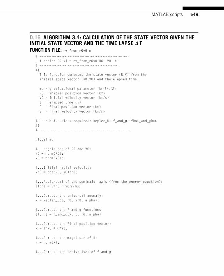
D.16 ALGORITHM 3.4: CALCULATION OF THE STATE VECTOR GIVEN THEINITIAL STATE VECTOR AND THE TIME LAPSE ΔTFUNCTION FILE: rv_from_r0v0.m
% �����������������������������������function [R,V] = rv_from_r0v0(R0, V0, t)
% �������������������������������%{
This function computes the state vector (R,V) from the
initial state vector (R0,V0) and the elapsed time.
mu - gravitational parameter (km 3̂/s 2̂)
R0 - initial position vector (km)
V0 - initial velocity vector (km/s)
t - elapsed time (s)
R - final position vector (km)
V - final velocity vector (km/s)
% User M-functions required: kepler_U, f_and_g, fDot_and_gDot
%}
% ––––––––––––––––––––––––––––––––––––––––––––––
global mu
%...Magnitudes of R0 and V0:
r0 = norm(R0);
v0 = norm(V0);
%...Initial radial velocity:
vr0 = dot(R0, V0)/r0;
%...Reciprocal of the semimajor axis (from the energy equation):
alpha = 2/r0 - v0 2̂/mu;
%...Compute the universal anomaly:
x = kepler_U(t, r0, vr0, alpha);
%...Compute the f and g functions:
[f, g] = f_and_g(x, t, r0, alpha);
%...Compute the final position vector:
R = f*R0 + g*V0;
%...Compute the magnitude of R:
r = norm(R);
%...Compute the derivatives of f and g:
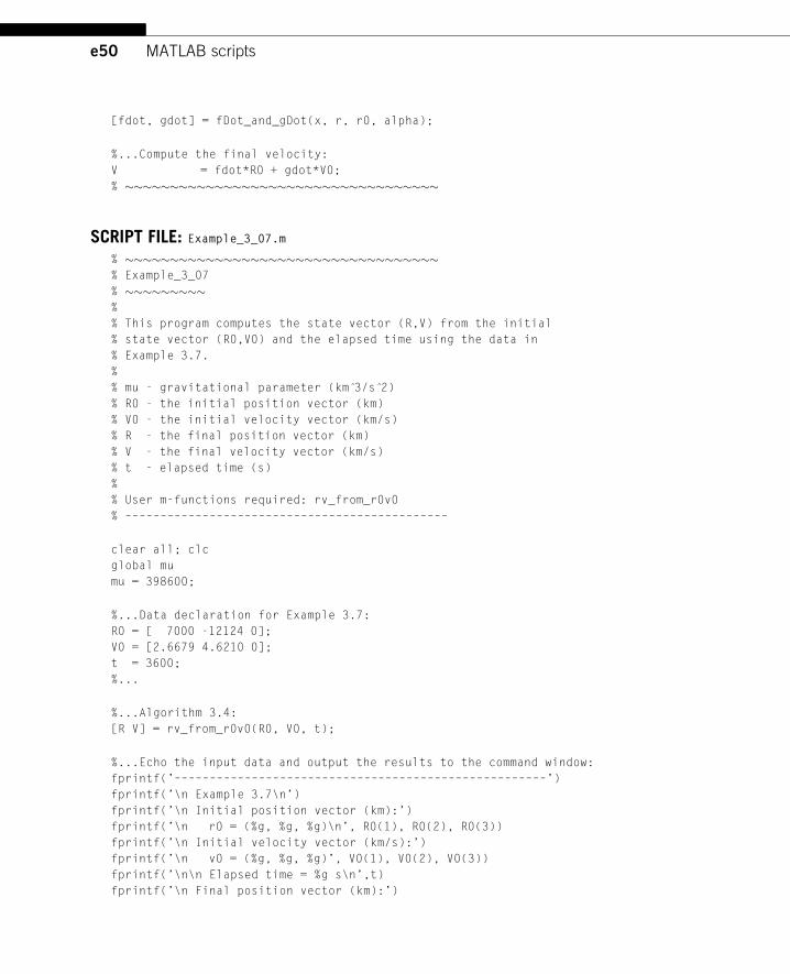
e50 MATLAB scripts
[fdot, gdot] = fDot_and_gDot(x, r, r0, alpha);
%...Compute the final velocity:
V = fdot*R0 + gdot*V0;
% �����������������������������������
SCRIPT FILE: Example_3_07.m
% �����������������������������������% Example_3_07
% ���������%
% This program computes the state vector (R,V) from the initial
% state vector (R0,V0) and the elapsed time using the data in
% Example 3.7.
%
% mu - gravitational parameter (km 3̂/s 2̂)
% R0 - the initial position vector (km)
% V0 - the initial velocity vector (km/s)
% R - the final position vector (km)
% V - the final velocity vector (km/s)
% t - elapsed time (s)
%
% User m-functions required: rv_from_r0v0
% ––––––––––––––––––––––––––––––––––––––––––––––
clear all; clc
global mu
mu = 398600;
%...Data declaration for Example 3.7:
R0 = [ 7000 -12124 0];
V0 = [2.6679 4.6210 0];
t = 3600;
%...
%...Algorithm 3.4:
[R V] = rv_from_r0v0(R0, V0, t);
%...Echo the input data and output the results to the command window:
fprintf(’–––––––––––––––––––––––––––––––––––––––––––––––––––––’)
fprintf(’\n Example 3.7\n’)
fprintf(’\n Initial position vector (km):’)
fprintf(’\n r0 = (%g, %g, %g)\n’, R0(1), R0(2), R0(3))
fprintf(’\n Initial velocity vector (km/s):’)
fprintf(’\n v0 = (%g, %g, %g)’, V0(1), V0(2), V0(3))
fprintf(’\n\n Elapsed time = %g s\n’,t)
fprintf(’\n Final position vector (km):’)
e51MATLAB scripts
fprintf(’\n r = (%g, %g, %g)\n’, R(1), R(2), R(3))
fprintf(’\n Final velocity vector (km/s):’)
fprintf(’\n v = (%g, %g, %g)’, V(1), V(2), V(3))
fprintf(’\n–––––––––––––––––––––––––––––––––––––––––––––––––––––\n’)
% �����������������������������������
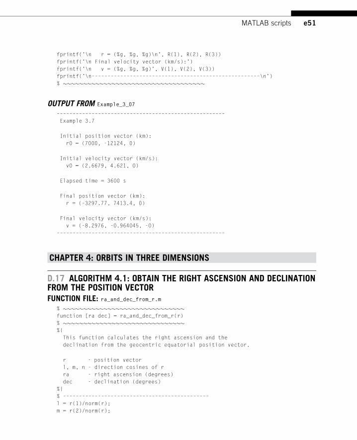
OUTPUT FROM Example_3_07
–––––––––––––––––––––––––––––––––––––––––––––––––––––
Example 3.7
Initial position vector (km):
r0 = (7000, -12124, 0)
Initial velocity vector (km/s):
v0 = (2.6679, 4.621, 0)
Elapsed time = 3600 s
Final position vector (km):
r = (-3297.77, 7413.4, 0)
Final velocity vector (km/s):
v = (-8.2976, -0.964045, -0)
–––––––––––––––––––––––––––––––––––––––––––––––––––––
CHAPTER 4: ORBITS IN THREE DIMENSIONS
D.17 ALGORITHM 4.1: OBTAIN THE RIGHT ASCENSION AND DECLINATIONFROM THE POSITION VECTORFUNCTION FILE: ra_and_dec_from_r.m
% ������������������������������function [ra dec] = ra_and_dec_from_r(r)
% ������������������������������%{
This function calculates the right ascension and the
declination from the geocentric equatorial position vector.
r - position vector
l, m, n - direction cosines of r
ra - right ascension (degrees)
dec - declination (degrees)
%}
% ––––––––––––––––––––––––––––––––––––––––––––––
l = r(1)/norm(r);
m = r(2)/norm(r);
e52 MATLAB scripts
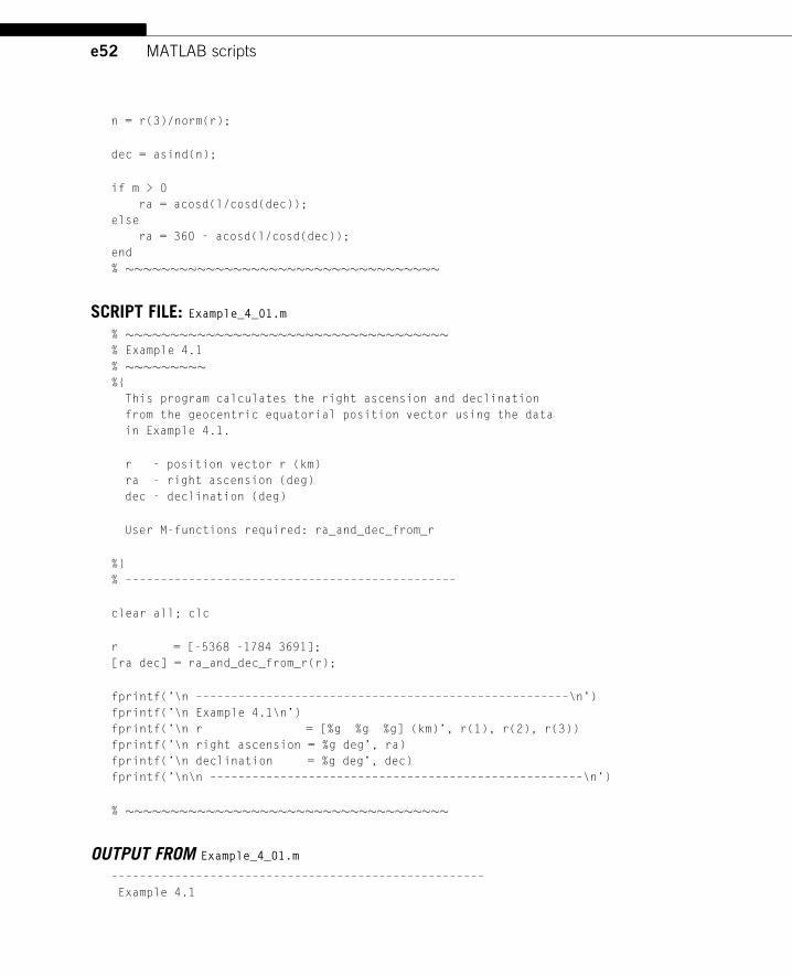
n = r(3)/norm(r);
dec = asind(n);
if m > 0
ra = acosd(l/cosd(dec));
else
ra = 360 - acosd(l/cosd(dec));
end
% �����������������������������������
SCRIPT FILE: Example_4_01.m
% ������������������������������������% Example 4.1
% ���������%{
This program calculates the right ascension and declination
from the geocentric equatorial position vector using the data
in Example 4.1.
r - position vector r (km)
ra - right ascension (deg)
dec - declination (deg)
User M-functions required: ra_and_dec_from_r
%}
% –––––––––––––––––––––––––––––––––––––––––––––––
clear all; clc
r = [-5368 -1784 3691];
[ra dec] = ra_and_dec_from_r(r);
fprintf(’\n –––––––––––––––––––––––––––––––––––––––––––––––––––––\n’)
fprintf(’\n Example 4.1\n’)
fprintf(’\n r = [%g %g %g] (km)’, r(1), r(2), r(3))
fprintf(’\n right ascension = %g deg’, ra)
fprintf(’\n declination = %g deg’, dec)
fprintf(’\n\n –––––––––––––––––––––––––––––––––––––––––––––––––––––\n’)
% ������������������������������������
OUTPUT FROM Example_4_01.m
–––––––––––––––––––––––––––––––––––––––––––––––––––––
Example 4.1
e53MATLAB scripts
r = [-5368 -1784 3691] (km)
right ascension = 198.384 deg
declination = 33.1245 deg
–––––––––––––––––––––––––––––––––––––––––––––––––––––
D.18 ALGORITHM 4.2: CALCULATION OF THE ORBITAL ELEMENTS FROMTHE STATE VECTORFUNCTION FILE: coe_from_sv.m
% ����������������������������������function coe = coe_from_sv(R,V,mu)
% ���������������������������%{
% This function computes the classical orbital elements (coe)
% from the state vector (R,V) using Algorithm 4.1.
%
mu - gravitational parameter (km 3̂/s 2̂)
R - position vector in the geocentric equatorial frame (km)
V - velocity vector in the geocentric equatorial frame (km)
r, v - the magnitudes of R and V
vr - radial velocity component (km/s)
H - the angular momentum vector (km 2̂/s)
h - the magnitude of H (km 2̂/s)
incl - inclination of the orbit (rad)
N - the node line vector (km 2̂/s)
n - the magnitude of N
cp - cross product of N and R
RA - right ascension of the ascending node (rad)
E - eccentricity vector
e - eccentricity (magnitude of E)
eps - a small number below which the eccentricity is considered
to be zero
w - argument of perigee (rad)
TA - true anomaly (rad)
a - semimajor axis (km)
pi - 3.1415926...
coe - vector of orbital elements [h e RA incl w TA a]
User M-functions required: None
%}
% –––––––––––––––––––––––––––––––––––––––––––––
eps = 1.e-10;
r = norm(R);
v = norm(V);
e54 MATLAB scripts
vr = dot(R,V)/r;
H = cross(R,V);
h = norm(H);
%...Equation 4.7:
incl = acos(H(3)/h);
%...Equation 4.8:
N = cross([0 0 1],H);
n = norm(N);
%...Equation 4.9:
if n �= 0
RA = acos(N(1)/n);
if N(2) < 0
RA = 2*pi - RA;
end
else
RA = 0;
end
%...Equation 4.10:
E = 1/mu*((v 2̂ - mu/r)*R - r*vr*V);
e = norm(E);
%...Equation 4.12 (incorporating the case e = 0):
if n �= 0
if e > eps
w = acos(dot(N,E)/n/e);
if E(3) < 0
w = 2*pi - w;
end
else
w = 0;
end
else
w = 0;
end
%...Equation 4.13a (incorporating the case e = 0):
if e > eps
TA = acos(dot(E,R)/e/r);
if vr < 0
TA = 2*pi - TA;
end
else
e55MATLAB scripts
cp = cross(N,R);
if cp(3) >= 0
TA = acos(dot(N,R)/n/r);
else
TA = 2*pi - acos(dot(N,R)/n/r);
end
end
%...Equation 4.62 (a < 0 for a hyperbola):
a = h 2̂/mu/(1 - e 2̂);
coe = [h e RA incl w TA a];
end %coe_from_sv
% ����������������������������������
SCRIPT FILE: Example_4_03.m
% �����������������������������������% Example_4_03
% ����������%{
This program uses Algorithm 4.2 to obtain the orbital
elements from the state vector provided in Example 4.3.
pi - 3.1415926...
deg - factor for converting between degrees and radians
mu - gravitational parameter (km 3̂/s 2̂)
r - position vector (km) in the geocentric equatorial frame
v - velocity vector (km/s) in the geocentric equatorial frame
coe - orbital elements [h e RA incl w TA a]
where h = angular momentum (km 2̂/s)
e = eccentricity
RA = right ascension of the ascending node (rad)
incl = orbit inclination (rad)
w = argument of perigee (rad)
TA = true anomaly (rad)
a = semimajor axis (km)
T - Period of an elliptic orbit (s)
User M-function required: coe_from_sv
%}
% ––––––––––––––––––––––––––––––––––––––––––––––
clear all; clc
deg = pi/180;
mu = 398600;
%...Data declaration for Example 4.3:
e56 MATLAB scripts
r = [ -6045 -3490 2500];
v = [-3.457 6.618 2.533];
%...
%...Algorithm 4.2:
coe = coe_from_sv(r,v,mu);
%...Echo the input data and output results to the command window:
fprintf(’–––––––––––––––––––––––––––––––––––––––––––––––––––––’)
fprintf(’\n Example 4.3\n’)
fprintf(’\n Gravitational parameter (km 3̂/s 2̂) = %g\n’, mu)
fprintf(’\n State vector:\n’)
fprintf(’\n r (km) = [%g %g %g]’, ...
r(1), r(2), r(3))
fprintf(’\n v (km/s) = [%g %g %g]’, ...
v(1), v(2), v(3))
disp(’ ’)
fprintf(’\n Angular momentum (km 2̂/s) = %g’, coe(1))
fprintf(’\n Eccentricity = %g’, coe(2))
fprintf(’\n Right ascension (deg) = %g’, coe(3)/deg)
fprintf(’\n Inclination (deg) = %g’, coe(4)/deg)
fprintf(’\n Argument of perigee (deg) = %g’, coe(5)/deg)
fprintf(’\n True anomaly (deg) = %g’, coe(6)/deg)
fprintf(’\n Semimajor axis (km): = %g’, coe(7))
%...if the orbit is an ellipse, output its period (Equation 2.73):
if coe(2)<1
T = 2*pi/sqrt(mu)*coe(7) 1̂.5;
fprintf(’\n Period:’)
fprintf(’\n Seconds = %g’, T)
fprintf(’\n Minutes = %g’, T/60)
fprintf(’\n Hours = %g’, T/3600)
fprintf(’\n Days = %g’, T/24/3600)
end
fprintf(’\n–––––––––––––––––––––––––––––––––––––––––––––––––––––\n’)
% �����������������������������������
OUTPUT FROM Example_4_03
–––––––––––––––––––––––––––––––––––––––––––––––––––––
Example 4.3
Gravitational parameter (km 3̂/s 2̂) = 398600
State vector:
r (km) = [-6045 -3490 2500]
v (km/s) = [-3.457 6.618 2.533]
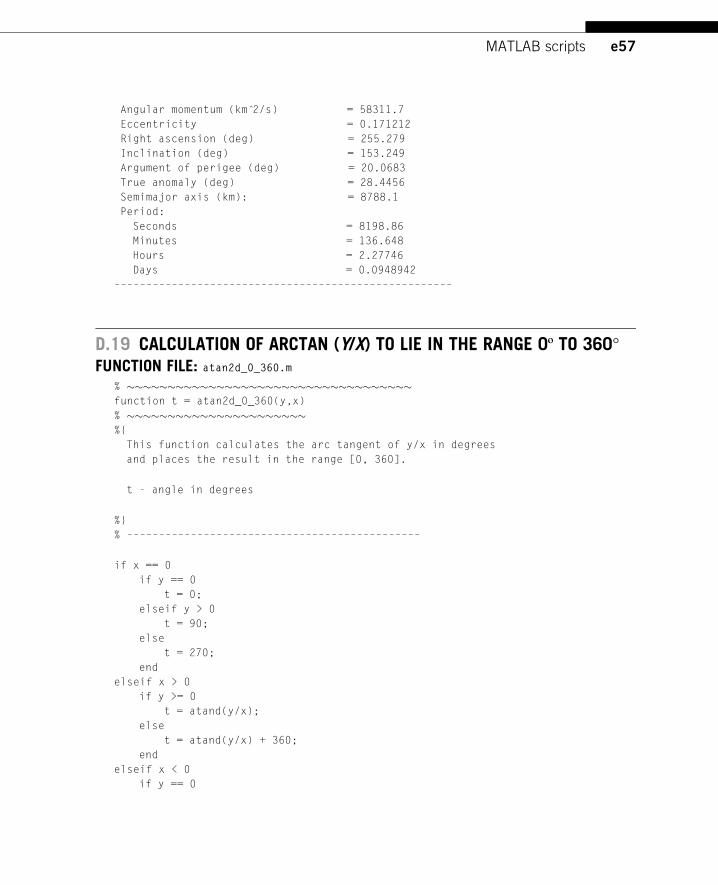
e57MATLAB scripts
Angular momentum (km 2̂/s) = 58311.7
Eccentricity = 0.171212
Right ascension (deg) = 255.279
Inclination (deg) = 153.249
Argument of perigee (deg) = 20.0683
True anomaly (deg) = 28.4456
Semimajor axis (km): = 8788.1
Period:
Seconds = 8198.86
Minutes = 136.648
Hours = 2.27746
Days = 0.0948942
–––––––––––––––––––––––––––––––––––––––––––––––––––––
D.19 CALCULATION OF ARCTAN (Y/X) TO LIE IN THE RANGE 0º TO 360°FUNCTION FILE: atan2d_0_360.m
% �����������������������������������function t = atan2d_0_360(y,x)
% ����������������������%{
This function calculates the arc tangent of y/x in degrees
and places the result in the range [0, 360].
t - angle in degrees
%}
% ––––––––––––––––––––––––––––––––––––––––––––––
if x == 0
if y == 0
t = 0;
elseif y > 0
t = 90;
else
t = 270;
end
elseif x > 0
if y >= 0
t = atand(y/x);
else
t = atand(y/x) + 360;
end
elseif x < 0
if y == 0
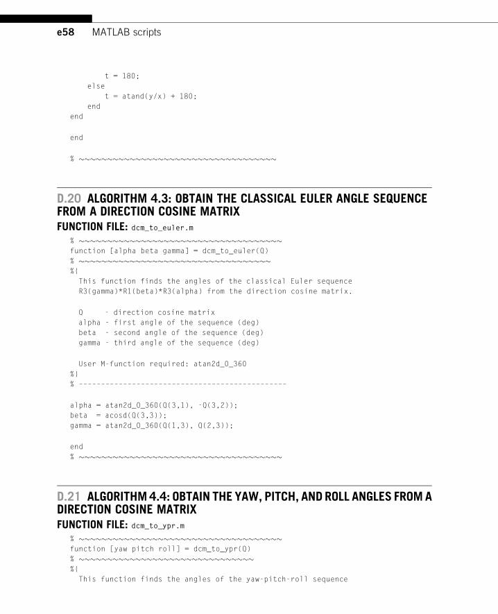
e58 MATLAB scripts
t = 180;
else
t = atand(y/x) + 180;
end
end
end
% �����������������������������������
D.20 ALGORITHM 4.3: OBTAIN THE CLASSICAL EULER ANGLE SEQUENCEFROM A DIRECTION COSINE MATRIXFUNCTION FILE: dcm_to_euler.m
% ������������������������������������function [alpha beta gamma] = dcm_to_euler(Q)
% ����������������������������������%{
This function finds the angles of the classical Euler sequence
R3(gamma)*R1(beta)*R3(alpha) from the direction cosine matrix.
Q - direction cosine matrix
alpha - first angle of the sequence (deg)
beta - second angle of the sequence (deg)
gamma - third angle of the sequence (deg)
User M-function required: atan2d_0_360
%}
% –––––––––––––––––––––––––––––––––––––––––––––––
alpha = atan2d_0_360(Q(3,1), -Q(3,2));
beta = acosd(Q(3,3));
gamma = atan2d_0_360(Q(1,3), Q(2,3));
end
% ������������������������������������
D.21 ALGORITHM4.4: OBTAIN THE YAW, PITCH, AND ROLL ANGLES FROMADIRECTION COSINE MATRIXFUNCTION FILE: dcm_to_ypr.m
% ������������������������������������function [yaw pitch roll] = dcm_to_ypr(Q)
% �������������������������������%{
This function finds the angles of the yaw-pitch-roll sequence
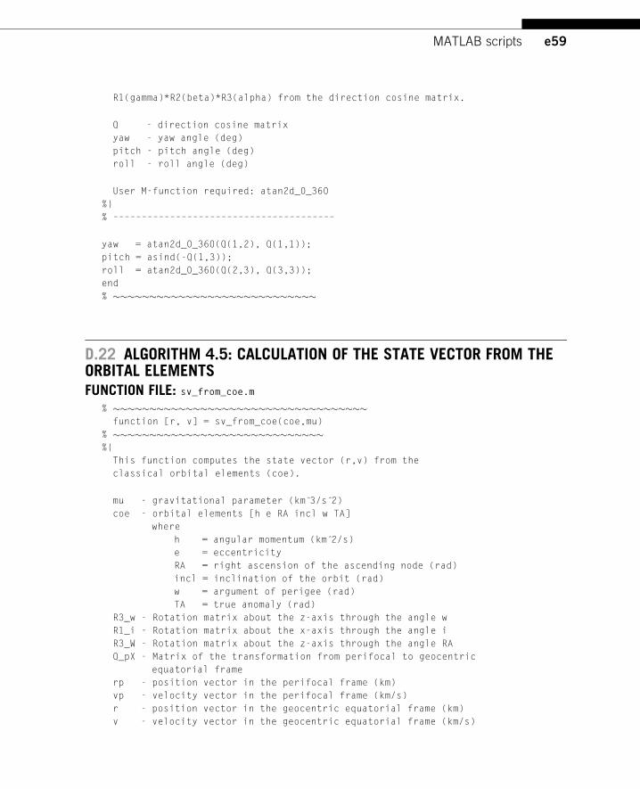
e59MATLAB scripts
R1(gamma)*R2(beta)*R3(alpha) from the direction cosine matrix.
Q - direction cosine matrix
yaw - yaw angle (deg)
pitch - pitch angle (deg)
roll - roll angle (deg)
User M-function required: atan2d_0_360
%}
% –––––––––––––––––––––––––––––––––––––––
yaw = atan2d_0_360(Q(1,2), Q(1,1));
pitch = asind(-Q(1,3));
roll = atan2d_0_360(Q(2,3), Q(3,3));
end
% ����������������������������
D.22 ALGORITHM 4.5: CALCULATION OF THE STATE VECTOR FROM THEORBITAL ELEMENTSFUNCTION FILE: sv_from_coe.m
% �����������������������������������function [r, v] = sv_from_coe(coe,mu)
% �����������������������������%{
This function computes the state vector (r,v) from the
classical orbital elements (coe).
mu - gravitational parameter (km 3̂/s 2̂)
coe - orbital elements [h e RA incl w TA]
where
h = angular momentum (km 2̂/s)
e = eccentricity
RA = right ascension of the ascending node (rad)
incl = inclination of the orbit (rad)
w = argument of perigee (rad)
TA = true anomaly (rad)
R3_w - Rotation matrix about the z-axis through the angle w
R1_i - Rotation matrix about the x-axis through the angle i
R3_W - Rotation matrix about the z-axis through the angle RA
Q_pX - Matrix of the transformation from perifocal to geocentric
equatorial frame
rp - position vector in the perifocal frame (km)
vp - velocity vector in the perifocal frame (km/s)
r - position vector in the geocentric equatorial frame (km)
v - velocity vector in the geocentric equatorial frame (km/s)
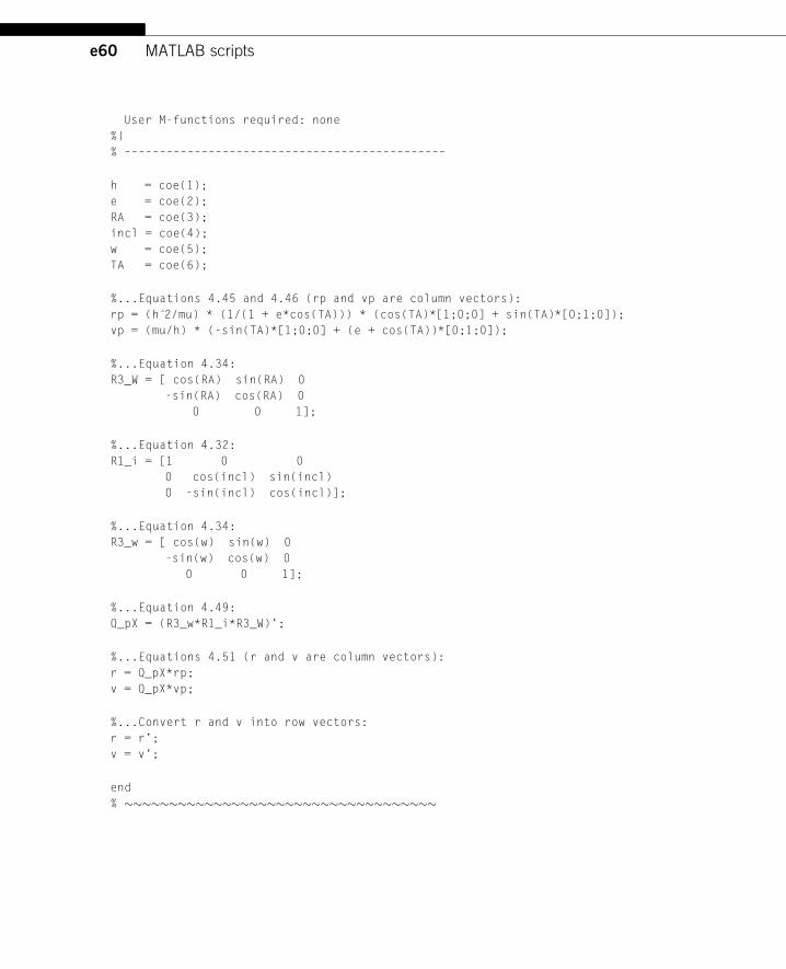
e60 MATLAB scripts
User M-functions required: none
%}
% ––––––––––––––––––––––––––––––––––––––––––––––
h = coe(1);
e = coe(2);
RA = coe(3);
incl = coe(4);
w = coe(5);
TA = coe(6);
%...Equations 4.45 and 4.46 (rp and vp are column vectors):
rp = (h 2̂/mu) * (1/(1 + e*cos(TA))) * (cos(TA)*[1;0;0] + sin(TA)*[0;1;0]);
vp = (mu/h) * (-sin(TA)*[1;0;0] + (e + cos(TA))*[0;1;0]);
%...Equation 4.34:
R3_W = [ cos(RA) sin(RA) 0
-sin(RA) cos(RA) 0
0 0 1];
%...Equation 4.32:
R1_i = [1 0 0
0 cos(incl) sin(incl)
0 -sin(incl) cos(incl)];
%...Equation 4.34:
R3_w = [ cos(w) sin(w) 0
-sin(w) cos(w) 0
0 0 1];
%...Equation 4.49:
Q_pX = (R3_w*R1_i*R3_W)’;
%...Equations 4.51 (r and v are column vectors):
r = Q_pX*rp;
v = Q_pX*vp;
%...Convert r and v into row vectors:
r = r’;
v = v’;
end
% �����������������������������������
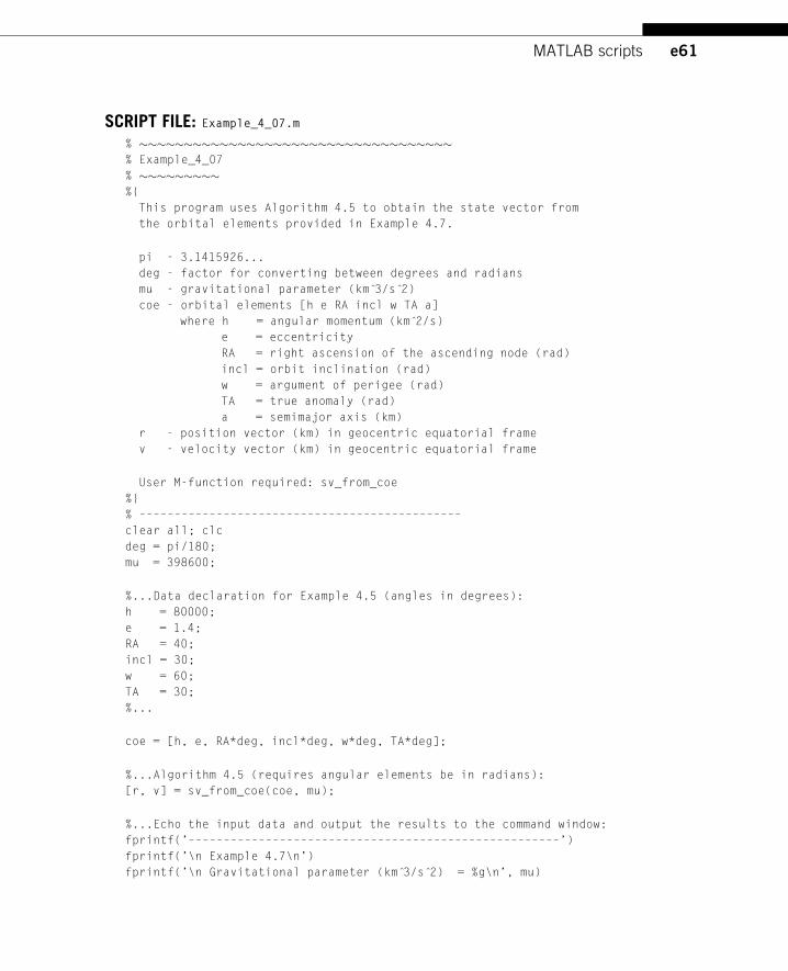
e61MATLAB scripts
SCRIPT FILE: Example_4_07.m
% �����������������������������������% Example_4_07
% ���������%{
This program uses Algorithm 4.5 to obtain the state vector from
the orbital elements provided in Example 4.7.
pi - 3.1415926...
deg - factor for converting between degrees and radians
mu - gravitational parameter (km 3̂/s 2̂)
coe - orbital elements [h e RA incl w TA a]
where h = angular momentum (km 2̂/s)
e = eccentricity
RA = right ascension of the ascending node (rad)
incl = orbit inclination (rad)
w = argument of perigee (rad)
TA = true anomaly (rad)
a = semimajor axis (km)
r - position vector (km) in geocentric equatorial frame
v - velocity vector (km) in geocentric equatorial frame
User M-function required: sv_from_coe
%}
% ––––––––––––––––––––––––––––––––––––––––––––––
clear all; clc
deg = pi/180;
mu = 398600;
%...Data declaration for Example 4.5 (angles in degrees):
h = 80000;
e = 1.4;
RA = 40;
incl = 30;
w = 60;
TA = 30;
%...
coe = [h, e, RA*deg, incl*deg, w*deg, TA*deg];
%...Algorithm 4.5 (requires angular elements be in radians):
[r, v] = sv_from_coe(coe, mu);
%...Echo the input data and output the results to the command window:
fprintf(’–––––––––––––––––––––––––––––––––––––––––––––––––––––’)
fprintf(’\n Example 4.7\n’)
fprintf(’\n Gravitational parameter (km 3̂/s 2̂) = %g\n’, mu)
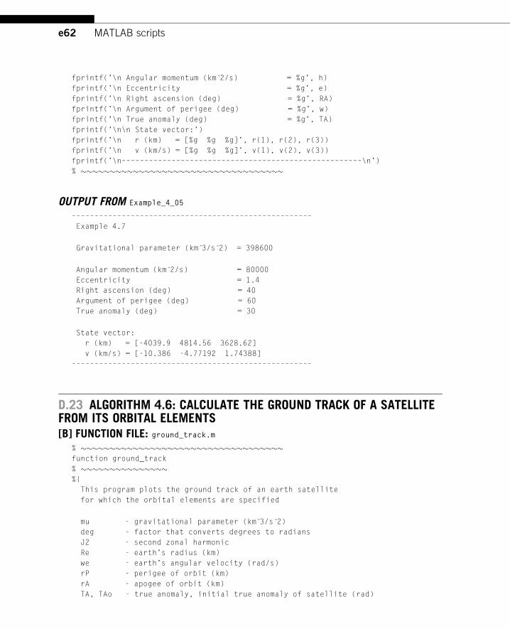
e62 MATLAB scripts
fprintf(’\n Angular momentum (km 2̂/s) = %g’, h)
fprintf(’\n Eccentricity = %g’, e)
fprintf(’\n Right ascension (deg) = %g’, RA)
fprintf(’\n Argument of perigee (deg) = %g’, w)
fprintf(’\n True anomaly (deg) = %g’, TA)
fprintf(’\n\n State vector:’)
fprintf(’\n r (km) = [%g %g %g]’, r(1), r(2), r(3))
fprintf(’\n v (km/s) = [%g %g %g]’, v(1), v(2), v(3))
fprintf(’\n–––––––––––––––––––––––––––––––––––––––––––––––––––––\n’)
% �����������������������������������
OUTPUT FROM Example_4_05
–––––––––––––––––––––––––––––––––––––––––––––––––––––
Example 4.7
Gravitational parameter (km 3̂/s 2̂) = 398600
Angular momentum (km 2̂/s) = 80000
Eccentricity = 1.4
Right ascension (deg) = 40
Argument of perigee (deg) = 60
True anomaly (deg) = 30
State vector:
r (km) = [-4039.9 4814.56 3628.62]
v (km/s) = [-10.386 -4.77192 1.74388]
–––––––––––––––––––––––––––––––––––––––––––––––––––––
D.23 ALGORITHM 4.6: CALCULATE THE GROUND TRACK OF A SATELLITEFROM ITS ORBITAL ELEMENTS[B] FUNCTION FILE: ground_track.m
% �����������������������������������function ground_track
% ���������������%{
This program plots the ground track of an earth satellite
for which the orbital elements are specified
mu - gravitational parameter (km 3̂/s 2̂)
deg - factor that converts degrees to radians
J2 - second zonal harmonic
Re - earth’s radius (km)
we - earth’s angular velocity (rad/s)
rP - perigee of orbit (km)
rA - apogee of orbit (km)
TA, TAo - true anomaly, initial true anomaly of satellite (rad)
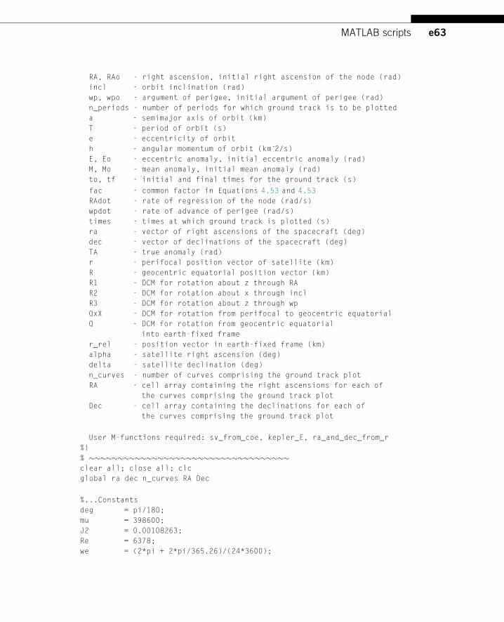
e63MATLAB scripts
RA, RAo - right ascension, initial right ascension of the node (rad)
incl - orbit inclination (rad)
wp, wpo - argument of perigee, initial argument of perigee (rad)
n_periods - number of periods for which ground track is to be plotted
a - semimajor axis of orbit (km)
T - period of orbit (s)
e - eccentricity of orbit
h - angular momentum of orbit (km 2̂/s)
E, Eo - eccentric anomaly, initial eccentric anomaly (rad)
M, Mo - mean anomaly, initial mean anomaly (rad)
to, tf - initial and final times for the ground track (s)
fac - common factor in Equations 4.53 and 4.53
RAdot - rate of regression of the node (rad/s)
wpdot - rate of advance of perigee (rad/s)
times - times at which ground track is plotted (s)
ra - vector of right ascensions of the spacecraft (deg)
dec - vector of declinations of the spacecraft (deg)
TA - true anomaly (rad)
r - perifocal position vector of satellite (km)
R - geocentric equatorial position vector (km)
R1 - DCM for rotation about z through RA
R2 - DCM for rotation about x through incl
R3 - DCM for rotation about z through wp
QxX - DCM for rotation from perifocal to geocentric equatorial
Q - DCM for rotation from geocentric equatorial
into earth-fixed frame
r_rel - position vector in earth-fixed frame (km)
alpha - satellite right ascension (deg)
delta - satellite declination (deg)
n_curves - number of curves comprising the ground track plot
RA - cell array containing the right ascensions for each of
the curves comprising the ground track plot
Dec - cell array containing the declinations for each of
the curves comprising the ground track plot
User M-functions required: sv_from_coe, kepler_E, ra_and_dec_from_r
%}
% �����������������������������������clear all; close all; clc
global ra dec n_curves RA Dec
%...Constants
deg = pi/180;
mu = 398600;
J2 = 0.00108263;
Re = 6378;
we = (2*pi + 2*pi/365.26)/(24*3600);
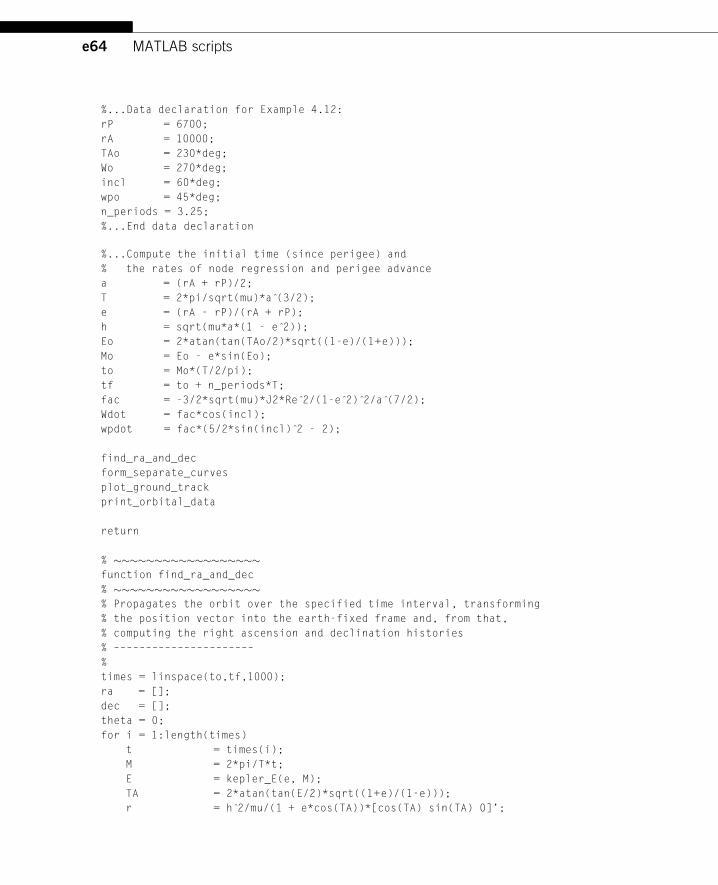
e64 MATLAB scripts
%...Data declaration for Example 4.12:
rP = 6700;
rA = 10000;
TAo = 230*deg;
Wo = 270*deg;
incl = 60*deg;
wpo = 45*deg;
n_periods = 3.25;
%...End data declaration
%...Compute the initial time (since perigee) and
% the rates of node regression and perigee advance
a = (rA + rP)/2;
T = 2*pi/sqrt(mu)*a (̂3/2);
e = (rA - rP)/(rA + rP);
h = sqrt(mu*a*(1 - e 2̂));
Eo = 2*atan(tan(TAo/2)*sqrt((1-e)/(1+e)));
Mo = Eo - e*sin(Eo);
to = Mo*(T/2/pi);
tf = to + n_periods*T;
fac = -3/2*sqrt(mu)*J2*Re 2̂/(1-e 2̂) 2̂/a (̂7/2);
Wdot = fac*cos(incl);
wpdot = fac*(5/2*sin(incl) 2̂ - 2);
find_ra_and_dec
form_separate_curves
plot_ground_track
print_orbital_data
return
% ������������������function find_ra_and_dec
% ������������������% Propagates the orbit over the specified time interval, transforming
% the position vector into the earth-fixed frame and, from that,
% computing the right ascension and declination histories
% ––––––––––––––––––––––
%
times = linspace(to,tf,1000);
ra = [];
dec = [];
theta = 0;
for i = 1:length(times)
t = times(i);
M = 2*pi/T*t;
E = kepler_E(e, M);
TA = 2*atan(tan(E/2)*sqrt((1+e)/(1-e)));
r = h 2̂/mu/(1 + e*cos(TA))*[cos(TA) sin(TA) 0]’;
e65MATLAB scripts
W = Wo + Wdot*t;
wp = wpo + wpdot*t;
R1 = [ cos(W) sin(W) 0
-sin(W) cos(W) 0
0 0 1];
R2 = [1 0 0
0 cos(incl) sin(incl)
0 -sin(incl) cos(incl)];
R3 = [ cos(wp) sin(wp) 0
-sin(wp) cos(wp) 0
0 0 1];
QxX = (R3*R2*R1)’;
R = QxX*r;
theta = we*(t - to);
Q = [ cos(theta) sin(theta) 0
-sin(theta) cos(theta) 0
0 0 1];
r_rel = Q*R;
[alpha delta] = ra_and_dec_from_r(r_rel);
ra = [ra; alpha];
dec = [dec; delta];
end
end %find_ra_and_dec
% ���������������������function form_separate_curves
% ���������������������% Breaks the ground track up into separate curves which start
% and terminate at right ascensions in the range [0,360 deg].
% –––––––––––––––––––––––––––
tol = 100;
curve_no = 1;
n_curves = 1;
k = 0;
ra_prev = ra(1);
for i = 1:length(ra)
if abs(ra(i) - ra_prev) > tol
e66 MATLAB scripts
curve_no = curve_no + 1;
n_curves = n_curves + 1;
k = 0;
end
k = k + 1;
RA{curve_no}(k) = ra(i);
Dec{curve_no}(k) = dec(i);
ra_prev = ra(i);
end
end %form_separate_curves
% �������������������function plot_ground_track
% �������������������hold on
xlabel(’East longitude (degrees)’)
ylabel(’Latitude (degrees)’)
axis equal
grid on
for i = 1:n_curves
plot(RA{i}, Dec{i})
end
axis ([0 360 -90 90])
text( ra(1), dec(1), ’o Start’)
text(ra(end), dec(end), ’o Finish’)
line([min(ra) max(ra)],[0 0], ’Color’,’k’) %the equator
end %plot_ground_track
% ��������������������function print_orbital_data
% ��������������������coe = [h e Wo incl wpo TAo];
[ro, vo] = sv_from_coe(coe, mu);
fprintf(’\n ––––––––––––––––––––––––––––––––––––––––––––––––––––\n’)
fprintf(’\n Angular momentum = %g km 2̂/s’ , h)
fprintf(’\n Eccentricity = %g’ , e)
fprintf(’\n Semimajor axis = %g km’ , a)
fprintf(’\n Perigee radius = %g km’ , rP)
fprintf(’\n Apogee radius = %g km’ , rA)
fprintf(’\n Period = %g hours’ , T/3600)
fprintf(’\n Inclination = %g deg’ , incl/deg)
fprintf(’\n Initial true anomaly = %g deg’ , TAo/deg)
fprintf(’\n Time since perigee = %g hours’ , to/3600)
fprintf(’\n Initial RA = %g deg’ , Wo/deg)
fprintf(’\n RA_dot = %g deg/period’ , Wdot/deg*T)
fprintf(’\n Initial wp = %g deg’ , wpo/deg)
e67MATLAB scripts
fprintf(’\n wp_dot = %g deg/period’ , wpdot/deg*T)
fprintf(’\n’)
fprintf(’\n r0 = [%12g, %12g, %12g] (km)’, ro(1), ro(2), ro(3))
fprintf(’\n magnitude = %g km\n’, norm(ro))
fprintf(’\n v0 = [%12g, %12g, %12g] (km)’, vo(1), vo(2), vo(3))
fprintf(’\n magnitude = %g km\n’, norm(vo))
fprintf(’\n ––––––––––––––––––––––––––––––––––––––––––––––––––––\n’)
end %print_orbital_data
end %ground_track
% �����������������������������������
CHAPTER 5: PRELIMINARY ORBIT DETERMINATION
D.24 ALGORITHM 5.1: GIBBS’ METHOD OF PRELIMINARY ORBITDETERMINATIONFUNCTION FILE: gibbs.m
% �������������������������������function [V2, ierr] = gibbs(R1, R2, R3)
% �������������������������������%{
This function uses the Gibbs method of orbit determination to
to compute the velocity corresponding to the second of three
supplied position vectors.
mu - gravitational parameter (km 3̂/s 2̂)
R1, R2, R3 - three coplanar geocentric position vectors (km)
r1, r2, r3 - the magnitudes of R1, R2 and R3 (km)
c12, c23, c31 - three independent cross products among
R1, R2 and R3
N, D, S - vectors formed from R1, R2 and R3 during
the Gibbs’ procedure
tol - tolerance for determining if R1, R2 and R3
are coplanar
ierr - = 0 if R1, R2, R3 are found to be coplanar
= 1 otherwise
V2 - the velocity corresponding to R2 (km/s)
User M-functions required: none
%}
% –––––––––––––––––––––––––––––––––––––––
global mu
tol = 1e-4;
ierr = 0;
e68 MATLAB scripts
%...Magnitudes of R1, R2 and R3:
r1 = norm(R1);
r2 = norm(R2);
r3 = norm(R3);
%...Cross products among R1, R2 and R3:
c12 = cross(R1,R2);
c23 = cross(R2,R3);
c31 = cross(R3,R1);
%...Check that R1, R2 and R3 are coplanar; if not set error flag:
if abs(dot(R1,c23)/r1/norm(c23)) > tol
ierr = 1;
end
%...Equation 5.13:
N = r1*c23 + r2*c31 + r3*c12;
%...Equation 5.14:
D = c12 + c23 + c31;
%...Equation 5.21:
S = R1*(r2 - r3) + R2*(r3 - r1) + R3*(r1 - r2);
%...Equation 5.22:
V2 = sqrt(mu/norm(N)/norm(D))*(cross(D,R2)/r2 + S);
% ����������������������������end %gibbs
SCRIPT FILE: Example_5_01.m
% �����������������������������������% Example_5_01
% ���������%{
This program uses Algorithm 5.1 (Gibbs method) and Algorithm 4.2
to obtain the orbital elements from the data provided in Example 5.1.
deg - factor for converting between degrees and radians
pi - 3.1415926...
mu - gravitational parameter (km 3̂/s 2̂)
r1, r2, r3 - three coplanar geocentric position vectors (km)
ierr - 0 if r1, r2, r3 are found to be coplanar
1 otherwise
v2 - the velocity corresponding to r2 (km/s)
coe - orbital elements [h e RA incl w TA a]
where h = angular momentum (km 2̂/s)
e = eccentricity
RA = right ascension of the ascending node (rad)
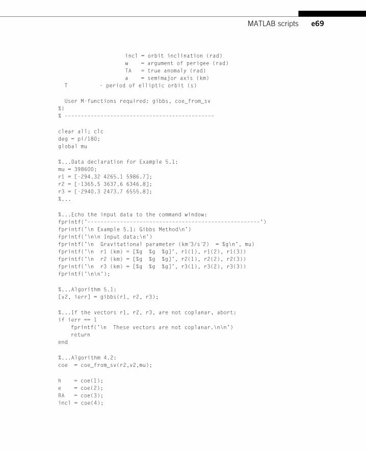
e69MATLAB scripts
incl = orbit inclination (rad)
w = argument of perigee (rad)
TA = true anomaly (rad)
a = semimajor axis (km)
T - period of elliptic orbit (s)
User M-functions required: gibbs, coe_from_sv
%}
% ––––––––––––––––––––––––––––––––––––––––––––––
clear all; clc
deg = pi/180;
global mu
%...Data declaration for Example 5.1:
mu = 398600;
r1 = [-294.32 4265.1 5986.7];
r2 = [-1365.5 3637.6 6346.8];
r3 = [-2940.3 2473.7 6555.8];
%...
%...Echo the input data to the command window:
fprintf(’–––––––––––––––––––––––––––––––––––––––––––––––––––––’)
fprintf(’\n Example 5.1: Gibbs Method\n’)
fprintf(’\n\n Input data:\n’)
fprintf(’\n Gravitational parameter (km 3̂/s 2̂) = %g\n’, mu)
fprintf(’\n r1 (km) = [%g %g %g]’, r1(1), r1(2), r1(3))
fprintf(’\n r2 (km) = [%g %g %g]’, r2(1), r2(2), r2(3))
fprintf(’\n r3 (km) = [%g %g %g]’, r3(1), r3(2), r3(3))
fprintf(’\n\n’);
%...Algorithm 5.1:
[v2, ierr] = gibbs(r1, r2, r3);
%...If the vectors r1, r2, r3, are not coplanar, abort:
if ierr == 1
fprintf(’\n These vectors are not coplanar.\n\n’)
return
end
%...Algorithm 4.2:
coe = coe_from_sv(r2,v2,mu);
h = coe(1);
e = coe(2);
RA = coe(3);
incl = coe(4);
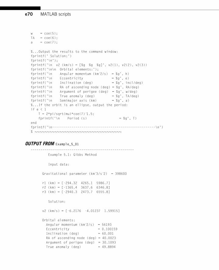
e70 MATLAB scripts
w = coe(5);
TA = coe(6);
a = coe(7);
%...Output the results to the command window:
fprintf(’ Solution:’)
fprintf(’\n’);
fprintf(’\n v2 (km/s) = [%g %g %g]’, v2(1), v2(2), v2(3))
fprintf(’\n\n Orbital elements:’);
fprintf(’\n Angular momentum (km 2̂/s) = %g’, h)
fprintf(’\n Eccentricity = %g’, e)
fprintf(’\n Inclination (deg) = %g’, incl/deg)
fprintf(’\n RA of ascending node (deg) = %g’, RA/deg)
fprintf(’\n Argument of perigee (deg) = %g’, w/deg)
fprintf(’\n True anomaly (deg) = %g’, TA/deg)
fprintf(’\n Semimajor axis (km) = %g’, a)
%...If the orbit is an ellipse, output the period:
if e < 1
T = 2*pi/sqrt(mu)*coe(7) 1̂.5;
fprintf(’\n Period (s) = %g’, T)
end
fprintf(’\n–––––––––––––––––––––––––––––––––––––––––––––––––––––\n’)
% �����������������������������������
OUTPUT FROM Example_5_01
–––––––––––––––––––––––––––––––––––––––––––––––––––––
Example 5.1: Gibbs Method
Input data:
Gravitational parameter (km 3̂/s 2̂) = 398600
r1 (km) = [-294.32 4265.1 5986.7]
r2 (km) = [-1365.4 3637.6 6346.8]
r3 (km) = [-2940.3 2473.7 6555.8]
Solution:
v2 (km/s) = [-6.2176 -4.01237 1.59915]
Orbital elements:
Angular momentum (km 2̂/s) = 56193
Eccentricity = 0.100159
Inclination (deg) = 60.001
RA of ascending node (deg) = 40.0023
Argument of perigee (deg) = 30.1093
True anomaly (deg) = 49.8894
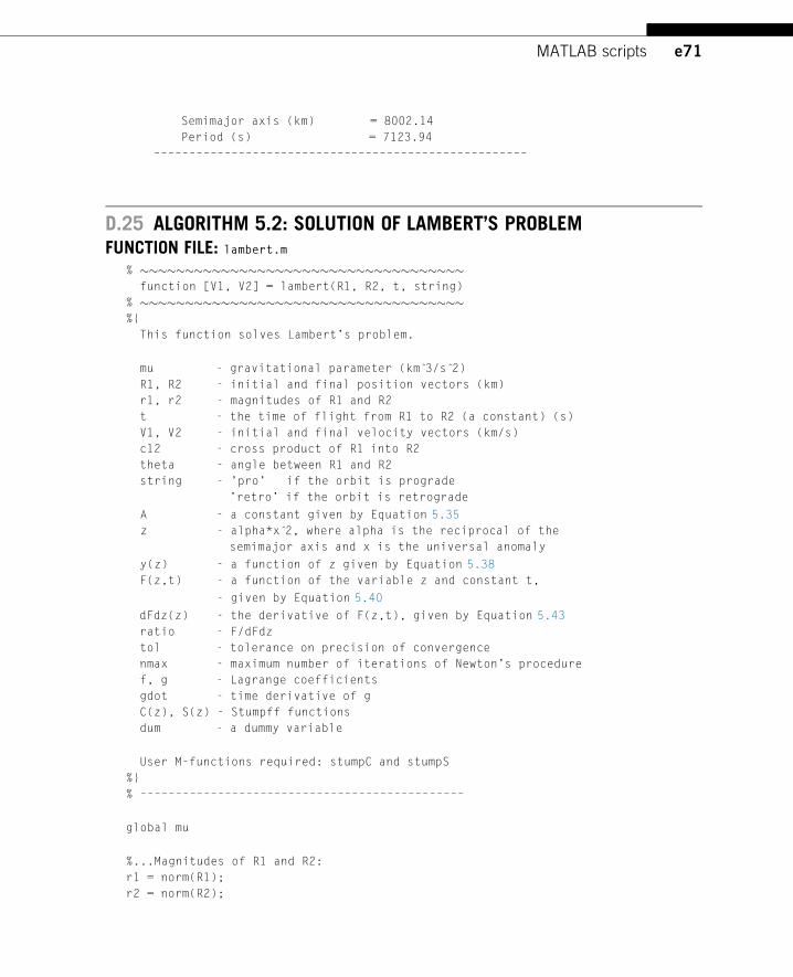
e71MATLAB scripts
Semimajor axis (km) = 8002.14
Period (s) = 7123.94
–––––––––––––––––––––––––––––––––––––––––––––––––––––
D.25 ALGORITHM 5.2: SOLUTION OF LAMBERT’S PROBLEMFUNCTION FILE: lambert.m
% ������������������������������������function [V1, V2] = lambert(R1, R2, t, string)
% ������������������������������������%{
This function solves Lambert’s problem.
mu - gravitational parameter (km 3̂/s 2̂)
R1, R2 - initial and final position vectors (km)
r1, r2 - magnitudes of R1 and R2
t - the time of flight from R1 to R2 (a constant) (s)
V1, V2 - initial and final velocity vectors (km/s)
c12 - cross product of R1 into R2
theta - angle between R1 and R2
string - ’pro’ if the orbit is prograde
’retro’ if the orbit is retrograde
A - a constant given by Equation 5.35
z - alpha*x 2̂, where alpha is the reciprocal of the
semimajor axis and x is the universal anomaly
y(z) - a function of z given by Equation 5.38
F(z,t) - a function of the variable z and constant t,
- given by Equation 5.40
dFdz(z) - the derivative of F(z,t), given by Equation 5.43
ratio - F/dFdz
tol - tolerance on precision of convergence
nmax - maximum number of iterations of Newton’s procedure
f, g - Lagrange coefficients
gdot - time derivative of g
C(z), S(z) - Stumpff functions
dum - a dummy variable
User M-functions required: stumpC and stumpS
%}
% ––––––––––––––––––––––––––––––––––––––––––––––
global mu
%...Magnitudes of R1 and R2:
r1 = norm(R1);
r2 = norm(R2);
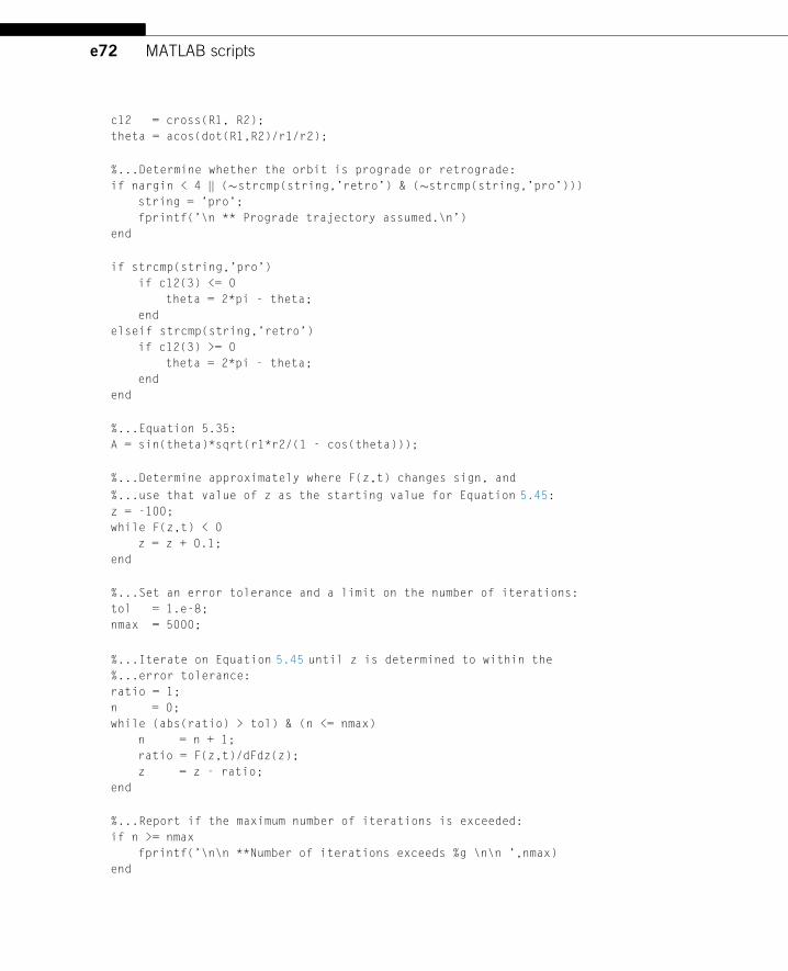
e72 MATLAB scripts
c12 = cross(R1, R2);
theta = acos(dot(R1,R2)/r1/r2);
%...Determine whether the orbit is prograde or retrograde:
if nargin < 4 jj (�strcmp(string,’retro’) & (�strcmp(string,’pro’)))
string = ’pro’;
fprintf(’\n ** Prograde trajectory assumed.\n’)
end
if strcmp(string,’pro’)
if c12(3) <= 0
theta = 2*pi - theta;
end
elseif strcmp(string,’retro’)
if c12(3) >= 0
theta = 2*pi - theta;
end
end
%...Equation 5.35:
A = sin(theta)*sqrt(r1*r2/(1 - cos(theta)));
%...Determine approximately where F(z,t) changes sign, and
%...use that value of z as the starting value for Equation 5.45:
z = -100;
while F(z,t) < 0
z = z + 0.1;
end
%...Set an error tolerance and a limit on the number of iterations:
tol = 1.e-8;
nmax = 5000;
%...Iterate on Equation 5.45 until z is determined to within the
%...error tolerance:
ratio = 1;
n = 0;
while (abs(ratio) > tol) & (n <= nmax)
n = n + 1;
ratio = F(z,t)/dFdz(z);
z = z - ratio;
end
%...Report if the maximum number of iterations is exceeded:
if n >= nmax
fprintf(’\n\n **Number of iterations exceeds %g \n\n ’,nmax)
end
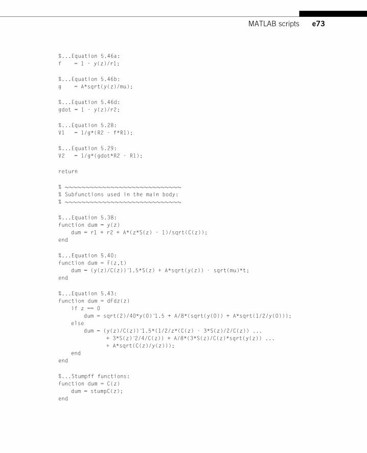
e73MATLAB scripts
%...Equation 5.46a:
f = 1 - y(z)/r1;
%...Equation 5.46b:
g = A*sqrt(y(z)/mu);
%...Equation 5.46d:
gdot = 1 - y(z)/r2;
%...Equation 5.28:
V1 = 1/g*(R2 - f*R1);
%...Equation 5.29:
V2 = 1/g*(gdot*R2 - R1);
return
% ����������������������������% Subfunctions used in the main body:
% ����������������������������
%...Equation 5.38:
function dum = y(z)
dum = r1 + r2 + A*(z*S(z) - 1)/sqrt(C(z));
end
%...Equation 5.40:
function dum = F(z,t)
dum = (y(z)/C(z)) 1̂.5*S(z) + A*sqrt(y(z)) - sqrt(mu)*t;
end
%...Equation 5.43:
function dum = dFdz(z)
if z == 0
dum = sqrt(2)/40*y(0) 1̂.5 + A/8*(sqrt(y(0)) + A*sqrt(1/2/y(0)));
else
dum = (y(z)/C(z)) 1̂.5*(1/2/z*(C(z) - 3*S(z)/2/C(z)) ...
+ 3*S(z) 2̂/4/C(z)) + A/8*(3*S(z)/C(z)*sqrt(y(z)) ...
+ A*sqrt(C(z)/y(z)));
end
end
%...Stumpff functions:
function dum = C(z)
dum = stumpC(z);
end
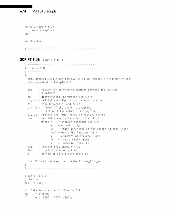
e74 MATLAB scripts
function dum = S(z)
dum = stumpS(z);
end
end %lambert
% �����������������������������������
SCRIPT FILE: Example_5_02.m
% ����������������������������������% Example_5_02
% ���������%{
This program uses Algorithm 5.2 to solve Lambert’s problem for the
data provided in Example 5.2.
deg - factor for converting between degrees and radians
pi - 3.1415926...
mu - gravitational parameter (km 3̂/s 2̂)
r1, r2 - initial and final position vectors (km)
dt - time between r1 and r2 (s)
string - = ’pro’ if the orbit is prograde
= ’retro if the orbit is retrograde
v1, v2 - initial and final velocity vectors (km/s)
coe - orbital elements [h e RA incl w TA a]
where h = angular momentum (km 2̂/s)
e = eccentricity
RA = right ascension of the ascending node (rad)
incl = orbit inclination (rad)
w = argument of perigee (rad)
TA = true anomaly (rad)
a = semimajor axis (km)
TA1 - Initial true anomaly (rad)
TA2 - Final true anomaly (rad)
T - period of an elliptic orbit (s)
User M-functions required: lambert, coe_from_sv
%}
% –––––––––––––––––––––––––––––––––––––––––––––
clear all; clc
global mu
deg = pi/180;
%...Data declaration for Example 5.2:
mu = 398600;
r1 = [ 5000 10000 2100];
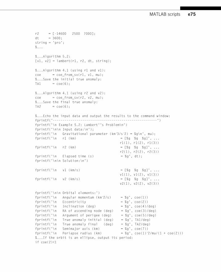
e75MATLAB scripts
r2 = [-14600 2500 7000];
dt = 3600;
string = ’pro’;
%...
%...Algorithm 5.2:
[v1, v2] = lambert(r1, r2, dt, string);
%...Algorithm 4.1 (using r1 and v1):
coe = coe_from_sv(r1, v1, mu);
%...Save the initial true anomaly:
TA1 = coe(6);
%...Algorithm 4.1 (using r2 and v2):
coe = coe_from_sv(r2, v2, mu);
%...Save the final true anomaly:
TA2 = coe(6);
%...Echo the input data and output the results to the command window:
fprintf(’–––––––––––––––––––––––––––––––––––––––––––––––––––––’)
fprintf(’\n Example 5.2: Lambert’’s Problem\n’)
fprintf(’\n\n Input data:\n’);
fprintf(’\n Gravitational parameter (km 3̂/s 2̂) = %g\n’, mu);
fprintf(’\n r1 (km) = [%g %g %g]’, ...
r1(1), r1(2), r1(3))
fprintf(’\n r2 (km) = [%g %g %g]’, ...
r2(1), r2(2), r2(3))
fprintf(’\n Elapsed time (s) = %g’, dt);
fprintf(’\n\n Solution:\n’)
fprintf(’\n v1 (km/s) = [%g %g %g]’, ...
v1(1), v1(2), v1(3))
fprintf(’\n v2 (km/s) = [%g %g %g]’, ...
v2(1), v2(2), v2(3))
fprintf(’\n\n Orbital elements:’)
fprintf(’\n Angular momentum (km 2̂/s) = %g’, coe(1))
fprintf(’\n Eccentricity = %g’, coe(2))
fprintf(’\n Inclination (deg) = %g’, coe(4)/deg)
fprintf(’\n RA of ascending node (deg) = %g’, coe(3)/deg)
fprintf(’\n Argument of perigee (deg) = %g’, coe(5)/deg)
fprintf(’\n True anomaly initial (deg) = %g’, TA1/deg)
fprintf(’\n True anomaly final (deg) = %g’, TA2/deg)
fprintf(’\n Semimajor axis (km) = %g’, coe(7))
fprintf(’\n Periapse radius (km) = %g’, coe(1) 2̂/mu/(1 + coe(2)))
%...If the orbit is an ellipse, output its period:
if coe(2)<1
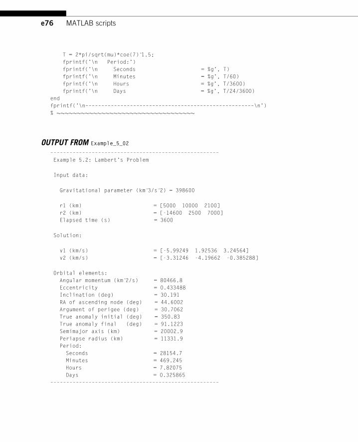
e76 MATLAB scripts
T = 2*pi/sqrt(mu)*coe(7) 1̂.5;
fprintf(’\n Period:’)
fprintf(’\n Seconds = %g’, T)
fprintf(’\n Minutes = %g’, T/60)
fprintf(’\n Hours = %g’, T/3600)
fprintf(’\n Days = %g’, T/24/3600)
end
fprintf(’\n–––––––––––––––––––––––––––––––––––––––––––––––––––––\n’)
% ����������������������������������
OUTPUT FROM Example_5_02
–––––––––––––––––––––––––––––––––––––––––––––––––––––
Example 5.2: Lambert’s Problem
Input data:
Gravitational parameter (km 3̂/s 2̂) = 398600
r1 (km) = [5000 10000 2100]
r2 (km) = [-14600 2500 7000]
Elapsed time (s) = 3600
Solution:
v1 (km/s) = [-5.99249 1.92536 3.24564]
v2 (km/s) = [-3.31246 -4.19662 -0.385288]
Orbital elements:
Angular momentum (km 2̂/s) = 80466.8
Eccentricity = 0.433488
Inclination (deg) = 30.191
RA of ascending node (deg) = 44.6002
Argument of perigee (deg) = 30.7062
True anomaly initial (deg) = 350.83
True anomaly final (deg) = 91.1223
Semimajor axis (km) = 20002.9
Periapse radius (km) = 11331.9
Period:
Seconds = 28154.7
Minutes = 469.245
Hours = 7.82075
Days = 0.325865
–––––––––––––––––––––––––––––––––––––––––––––––––––––
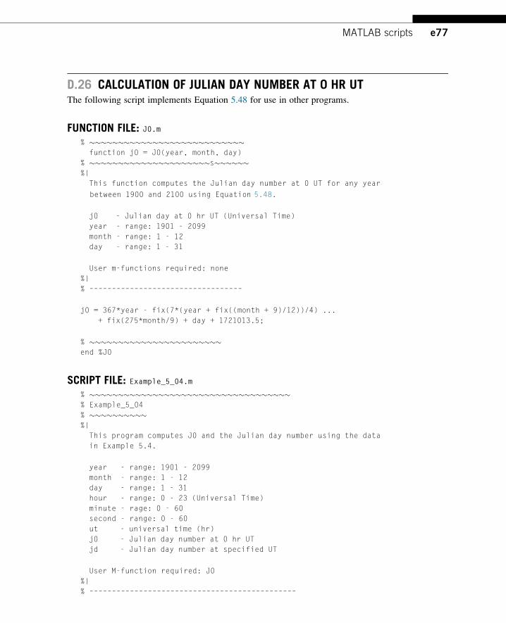
e77MATLAB scripts
D.26 CALCULATION OF JULIAN DAY NUMBER AT 0 HR UTThe following script implements Equation 5.48 for use in other programs.
FUNCTION FILE: J0.m
% ���������������������������function j0 = J0(year, month, day)
% ���������������������s������%{
This function computes the Julian day number at 0 UT for any year
between 1900 and 2100 using Equation 5.48.
j0 - Julian day at 0 hr UT (Universal Time)
year - range: 1901 - 2099
month - range: 1 - 12
day - range: 1 - 31
User m-functions required: none
%}
% ––––––––––––––––––––––––––––––––––
j0 = 367*year - fix(7*(year + fix((month + 9)/12))/4) ...
+ fix(275*month/9) + day + 1721013.5;
% �����������������������end %J0
SCRIPT FILE: Example_5_04.m
% �����������������������������������% Example_5_04
% ����������%{
This program computes J0 and the Julian day number using the data
in Example 5.4.
year - range: 1901 - 2099
month - range: 1 - 12
day - range: 1 - 31
hour - range: 0 - 23 (Universal Time)
minute - rage: 0 - 60
second - range: 0 - 60
ut - universal time (hr)
j0 - Julian day number at 0 hr UT
jd - Julian day number at specified UT
User M-function required: J0
%}
% ––––––––––––––––––––––––––––––––––––––––––––––
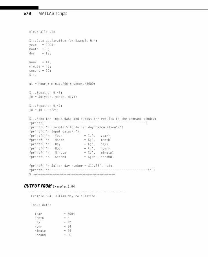
e78 MATLAB scripts
clear all; clc
%...Data declaration for Example 5.4:
year = 2004;
month = 5;
day = 12;
hour = 14;
minute = 45;
second = 30;
%...
ut = hour + minute/60 + second/3600;
%...Equation 5.46:
j0 = J0(year, month, day);
%...Equation 5.47:
jd = j0 + ut/24;
%...Echo the input data and output the results to the command window:
fprintf(’–––––––––––––––––––––––––––––––––––––––––––––––––––––’)
fprintf(’\n Example 5.4: Julian day calculation\n’)
fprintf(’\n Input data:\n’);
fprintf(’\n Year = %g’, year)
fprintf(’\n Month = %g’, month)
fprintf(’\n Day = %g’, day)
fprintf(’\n Hour = %g’, hour)
fprintf(’\n Minute = %g’, minute)
fprintf(’\n Second = %g\n’, second)
fprintf(’\n Julian day number = %11.3f’, jd);
fprintf(’\n–––––––––––––––––––––––––––––––––––––––––––––––––––––\n’)
% �����������������������������������
OUTPUT FROM Example_5_04
–––––––––––––––––––––––––––––––––––––––––––––––––––––
Example 5.4: Julian day calculation
Input data:
Year = 2004
Month = 5
Day = 12
Hour = 14
Minute = 45
Second = 30
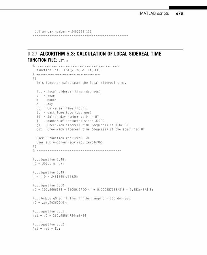
e79MATLAB scripts
Julian day number = 2453138.115
––––––––––––––––––––––––––––––––––––––––––––––––––––
D.27 ALGORITHM 5.3: CALCULATION OF LOCAL SIDEREAL TIMEFUNCTION FILE: LST.m
% �����������������������������������function lst = LST(y, m, d, ut, EL)
% ���������������������������%{
This function calculates the local sidereal time.
lst - local sidereal time (degrees)
y - year
m - month
d - day
ut - Universal Time (hours)
EL - east longitude (degrees)
j0 - Julian day number at 0 hr UT
j - number of centuries since J2000
g0 - Greenwich sidereal time (degrees) at 0 hr UT
gst - Greenwich sidereal time (degrees) at the specified UT
User M-function required: J0
User subfunction required: zeroTo360
%}
% ––––––––––––––––––––––––––––––––––––––––––––––
%...Equation 5.48;
j0 = J0(y, m, d);
%...Equation 5.49:
j = (j0 - 2451545)/36525;
%...Equation 5.50:
g0 = 100.4606184 + 36000.77004*j + 0.000387933*j 2̂ - 2.583e-8*j 3̂;
%...Reduce g0 so it lies in the range 0 - 360 degrees
g0 = zeroTo360(g0);
%...Equation 5.51:
gst = g0 + 360.98564724*ut/24;
%...Equation 5.52:
lst = gst + EL;
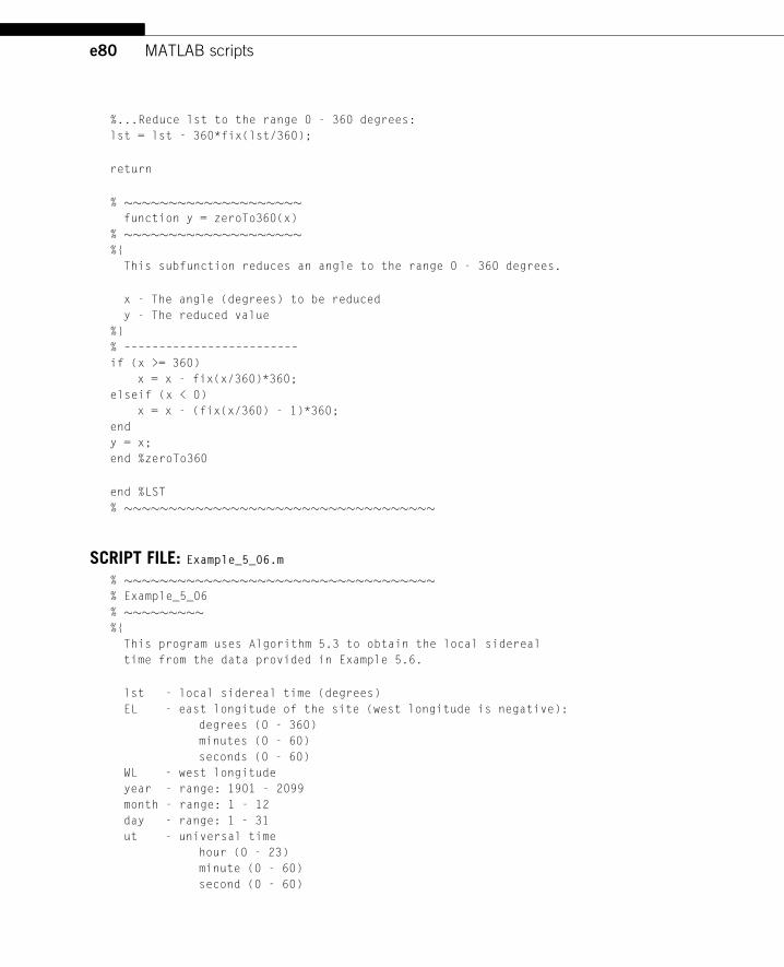
e80 MATLAB scripts
%...Reduce lst to the range 0 - 360 degrees:
lst = lst - 360*fix(lst/360);
return
% ��������������������function y = zeroTo360(x)
% ��������������������%{
This subfunction reduces an angle to the range 0 - 360 degrees.
x - The angle (degrees) to be reduced
y - The reduced value
%}
% –––––––––––––––––––––––––
if (x >= 360)
x = x - fix(x/360)*360;
elseif (x < 0)
x = x - (fix(x/360) - 1)*360;
end
y = x;
end %zeroTo360
end %LST
% �����������������������������������
SCRIPT FILE: Example_5_06.m
% �����������������������������������% Example_5_06
% ���������%{
This program uses Algorithm 5.3 to obtain the local sidereal
time from the data provided in Example 5.6.
lst - local sidereal time (degrees)
EL - east longitude of the site (west longitude is negative):
degrees (0 - 360)
minutes (0 - 60)
seconds (0 - 60)
WL - west longitude
year - range: 1901 - 2099
month - range: 1 - 12
day - range: 1 - 31
ut - universal time
hour (0 - 23)
minute (0 - 60)
second (0 - 60)
e81MATLAB scripts
User m-function required: LST
%}
% ––––––––––––––––––––––––––––––––––––––––––––––
clear all; clc
%...Data declaration for Example 5.6:
% East longitude:
degrees = 139;
minutes = 47;
seconds = 0;
% Date:
year = 2004;
month = 3;
day = 3;
% Universal time:
hour = 4;
minute = 30;
second = 0;
%...
%...Convert negative (west) longitude to east longitude:
if degrees < 0
degrees = degrees + 360;
end
%...Express the longitudes as decimal numbers:
EL = degrees + minutes/60 + seconds/3600;
WL = 360 - EL;
%...Express universal time as a decimal number:
ut = hour + minute/60 + second/3600;
%...Algorithm 5.3:
lst = LST(year, month, day, ut, EL);
%...Echo the input data and output the results to the command window:
fprintf(’–––––––––––––––––––––––––––––––––––––––––––––––––––––’)
fprintf(’\n Example 5.6: Local sidereal time calculation\n’)
fprintf(’\n Input data:\n’);
fprintf(’\n Year = %g’, year)
fprintf(’\n Month = %g’, month)
fprintf(’\n Day = %g’, day)
fprintf(’\n UT (hr) = %g’, ut)
fprintf(’\n West Longitude (deg) = %g’, WL)
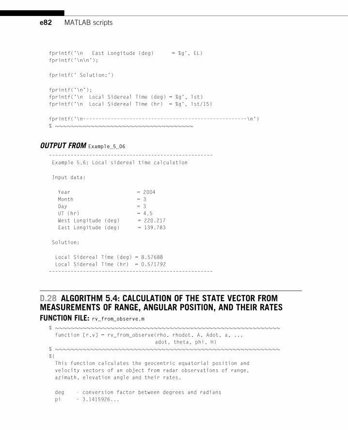
e82 MATLAB scripts
fprintf(’\n East Longitude (deg) = %g’, EL)
fprintf(’\n\n’);
fprintf(’ Solution:’)
fprintf(’\n’);
fprintf(’\n Local Sidereal Time (deg) = %g’, lst)
fprintf(’\n Local Sidereal Time (hr) = %g’, lst/15)
fprintf(’\n–––––––––––––––––––––––––––––––––––––––––––––––––––––\n’)
% �����������������������������������
OUTPUT FROM Example_5_06
–––––––––––––––––––––––––––––––––––––––––––––––––––––
Example 5.6: Local sidereal time calculation
Input data:
Year = 2004
Month = 3
Day = 3
UT (hr) = 4.5
West Longitude (deg) = 220.217
East Longitude (deg) = 139.783
Solution:
Local Sidereal Time (deg) = 8.57688
Local Sidereal Time (hr) = 0.571792
–––––––––––––––––––––––––––––––––––––––––––––––––––––
D.28 ALGORITHM 5.4: CALCULATION OF THE STATE VECTOR FROMMEASUREMENTS OF RANGE, ANGULAR POSITION, AND THEIR RATESFUNCTION FILE: rv_from_observe.m
% ���������������������������������������������������������function [r,v] = rv_from_observe(rho, rhodot, A, Adot, a, ...
adot, theta, phi, H)
% ���������������������������������������������������������%{
This function calculates the geocentric equatorial position and
velocity vectors of an object from radar observations of range,
azimuth, elevation angle and their rates.
deg - conversion factor between degrees and radians
pi - 3.1415926...
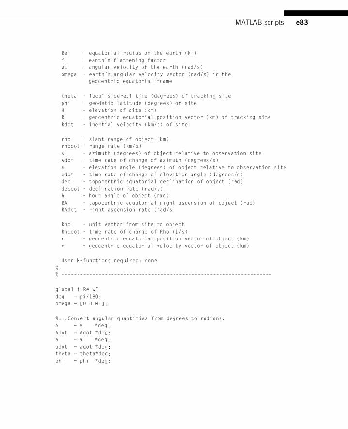
e83MATLAB scripts
Re - equatorial radius of the earth (km)
f - earth’s flattening factor
wE - angular velocity of the earth (rad/s)
omega - earth’s angular velocity vector (rad/s) in the
geocentric equatorial frame
theta - local sidereal time (degrees) of tracking site
phi - geodetic latitude (degrees) of site
H - elevation of site (km)
R - geocentric equatorial position vector (km) of tracking site
Rdot - inertial velocity (km/s) of site
rho - slant range of object (km)
rhodot - range rate (km/s)
A - azimuth (degrees) of object relative to observation site
Adot - time rate of change of azimuth (degrees/s)
a - elevation angle (degrees) of object relative to observation site
adot - time rate of change of elevation angle (degrees/s)
dec - topocentric equatorial declination of object (rad)
decdot - declination rate (rad/s)
h - hour angle of object (rad)
RA - topocentric equatorial right ascension of object (rad)
RAdot - right ascension rate (rad/s)
Rho - unit vector from site to object
Rhodot - time rate of change of Rho (1/s)
r - geocentric equatorial position vector of object (km)
v - geocentric equatorial velocity vector of object (km)
User M-functions required: none
%}
% ––––––––––––––––––––––––––––––––––––––––––––––––––––––––––––––––––––
global f Re wE
deg = pi/180;
omega = [0 0 wE];
%...Convert angular quantities from degrees to radians:
A = A *deg;
Adot = Adot *deg;
a = a *deg;
adot = adot *deg;
theta = theta*deg;
phi = phi *deg;
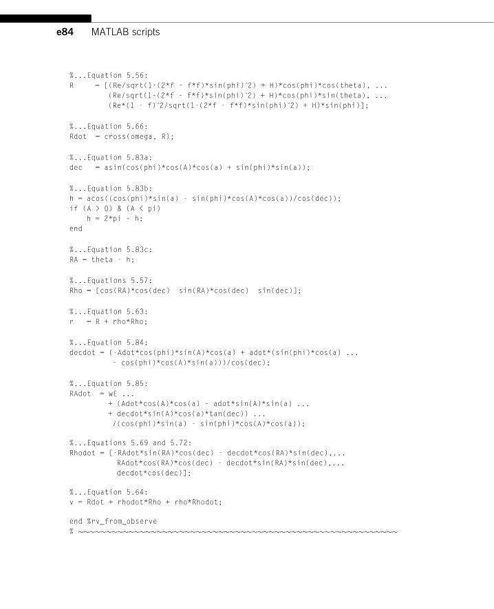
e84 MATLAB scripts
%...Equation 5.56:
R = [(Re/sqrt(1-(2*f - f*f)*sin(phi) 2̂) + H)*cos(phi)*cos(theta), ...
(Re/sqrt(1-(2*f - f*f)*sin(phi) 2̂) + H)*cos(phi)*sin(theta), ...
(Re*(1 - f) 2̂/sqrt(1-(2*f - f*f)*sin(phi) 2̂) + H)*sin(phi)];
%...Equation 5.66:
Rdot = cross(omega, R);
%...Equation 5.83a:
dec = asin(cos(phi)*cos(A)*cos(a) + sin(phi)*sin(a));
%...Equation 5.83b:
h = acos((cos(phi)*sin(a) - sin(phi)*cos(A)*cos(a))/cos(dec));
if (A > 0) & (A < pi)
h = 2*pi - h;
end
%...Equation 5.83c:
RA = theta - h;
%...Equations 5.57:
Rho = [cos(RA)*cos(dec) sin(RA)*cos(dec) sin(dec)];
%...Equation 5.63:
r = R + rho*Rho;
%...Equation 5.84:
decdot = (-Adot*cos(phi)*sin(A)*cos(a) + adot*(sin(phi)*cos(a) ...
- cos(phi)*cos(A)*sin(a)))/cos(dec);
%...Equation 5.85:
RAdot = wE ...
+ (Adot*cos(A)*cos(a) - adot*sin(A)*sin(a) ...
+ decdot*sin(A)*cos(a)*tan(dec)) ...
/(cos(phi)*sin(a) - sin(phi)*cos(A)*cos(a));
%...Equations 5.69 and 5.72:
Rhodot = [-RAdot*sin(RA)*cos(dec) - decdot*cos(RA)*sin(dec),...
RAdot*cos(RA)*cos(dec) - decdot*sin(RA)*sin(dec),...
decdot*cos(dec)];
%...Equation 5.64:
v = Rdot + rhodot*Rho + rho*Rhodot;
end %rv_from_observe
% ���������������������������������������������������������
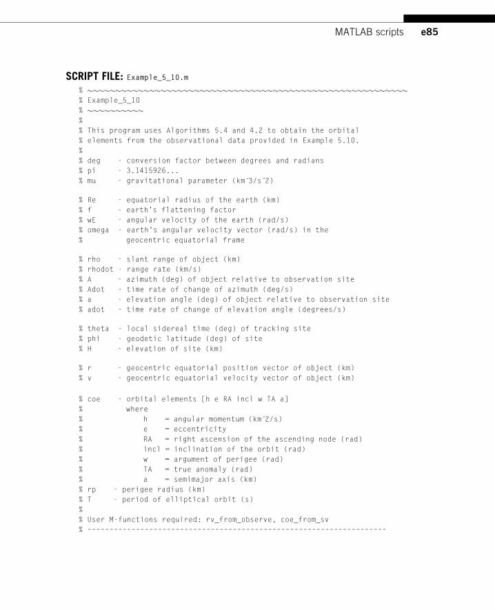
e85MATLAB scripts
SCRIPT FILE: Example_5_10.m
% ���������������������������������������������������������% Example_5_10
% ����������%
% This program uses Algorithms 5.4 and 4.2 to obtain the orbital
% elements from the observational data provided in Example 5.10.
%
% deg - conversion factor between degrees and radians
% pi - 3.1415926...
% mu - gravitational parameter (km 3̂/s 2̂)
% Re - equatorial radius of the earth (km)
% f - earth’s flattening factor
% wE - angular velocity of the earth (rad/s)
% omega - earth’s angular velocity vector (rad/s) in the
% geocentric equatorial frame
% rho - slant range of object (km)
% rhodot - range rate (km/s)
% A - azimuth (deg) of object relative to observation site
% Adot - time rate of change of azimuth (deg/s)
% a - elevation angle (deg) of object relative to observation site
% adot - time rate of change of elevation angle (degrees/s)
% theta - local sidereal time (deg) of tracking site
% phi - geodetic latitude (deg) of site
% H - elevation of site (km)
% r - geocentric equatorial position vector of object (km)
% v - geocentric equatorial velocity vector of object (km)
% coe - orbital elements [h e RA incl w TA a]
% where
% h = angular momentum (km 2̂/s)
% e = eccentricity
% RA = right ascension of the ascending node (rad)
% incl = inclination of the orbit (rad)
% w = argument of perigee (rad)
% TA = true anomaly (rad)
% a = semimajor axis (km)
% rp - perigee radius (km)
% T - period of elliptical orbit (s)
%
% User M-functions required: rv_from_observe, coe_from_sv
% ––––––––––––––––––––––––––––––––––––––––––––––––––––––––––––––––––––
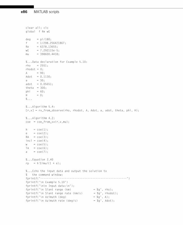
e86 MATLAB scripts
clear all; clc
global f Re wE
deg = pi/180;
f = 1/298.256421867;
Re = 6378.13655;
wE = 7.292115e-5;
mu = 398600.4418;
%...Data declaration for Example 5.10:
rho = 2551;
rhodot = 0;
A = 90;
Adot = 0.1130;
a = 30;
adot = 0.05651;
theta = 300;
phi = 60;
H = 0;
%...
%...Algorithm 5.4:
[r,v] = rv_from_observe(rho, rhodot, A, Adot, a, adot, theta, phi, H);
%...Algorithm 4.2:
coe = coe_from_sv(r,v,mu);
h = coe(1);
e = coe(2);
RA = coe(3);
incl = coe(4);
w = coe(5);
TA = coe(6);
a = coe(7);
%...Equation 2.40
rp = h 2̂/mu/(1 + e);
%...Echo the input data and output the solution to
% the command window:
fprintf(’–––––––––––––––––––––––––––––––––––––––––––––––––––––’)
fprintf(’\n Example 5.10’)
fprintf(’\n\n Input data:\n’);
fprintf(’\n Slant range (km) = %g’, rho);
fprintf(’\n Slant range rate (km/s) = %g’, rhodot);
fprintf(’\n Azimuth (deg) = %g’, A);
fprintf(’\n Azimuth rate (deg/s) = %g’, Adot);
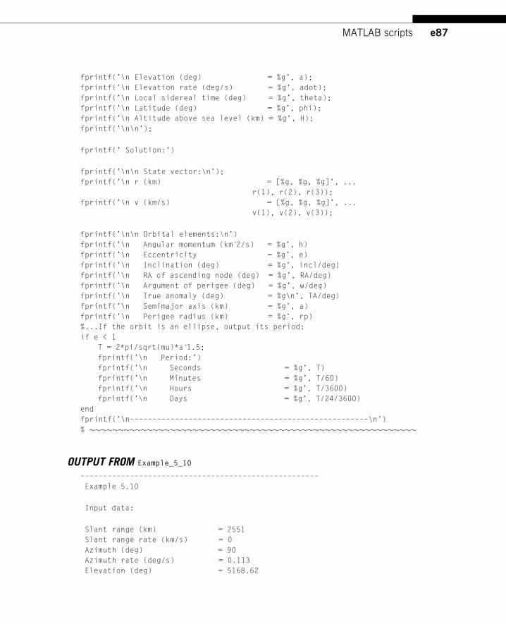
e87MATLAB scripts
fprintf(’\n Elevation (deg) = %g’, a);
fprintf(’\n Elevation rate (deg/s) = %g’, adot);
fprintf(’\n Local sidereal time (deg) = %g’, theta);
fprintf(’\n Latitude (deg) = %g’, phi);
fprintf(’\n Altitude above sea level (km) = %g’, H);
fprintf(’\n\n’);
fprintf(’ Solution:’)
fprintf(’\n\n State vector:\n’);
fprintf(’\n r (km) = [%g, %g, %g]’, ...
r(1), r(2), r(3));
fprintf(’\n v (km/s) = [%g, %g, %g]’, ...
v(1), v(2), v(3));
fprintf(’\n\n Orbital elements:\n’)
fprintf(’\n Angular momentum (km 2̂/s) = %g’, h)
fprintf(’\n Eccentricity = %g’, e)
fprintf(’\n Inclination (deg) = %g’, incl/deg)
fprintf(’\n RA of ascending node (deg) = %g’, RA/deg)
fprintf(’\n Argument of perigee (deg) = %g’, w/deg)
fprintf(’\n True anomaly (deg) = %g\n’, TA/deg)
fprintf(’\n Semimajor axis (km) = %g’, a)
fprintf(’\n Perigee radius (km) = %g’, rp)
%...If the orbit is an ellipse, output its period:
if e < 1
T = 2*pi/sqrt(mu)*a 1̂.5;
fprintf(’\n Period:’)
fprintf(’\n Seconds = %g’, T)
fprintf(’\n Minutes = %g’, T/60)
fprintf(’\n Hours = %g’, T/3600)
fprintf(’\n Days = %g’, T/24/3600)
end
fprintf(’\n–––––––––––––––––––––––––––––––––––––––––––––––––––––\n’)
% ���������������������������������������������������������
OUTPUT FROM Example_5_10
–––––––––––––––––––––––––––––––––––––––––––––––––––––
Example 5.10
Input data:
Slant range (km) = 2551
Slant range rate (km/s) = 0
Azimuth (deg) = 90
Azimuth rate (deg/s) = 0.113
Elevation (deg) = 5168.62
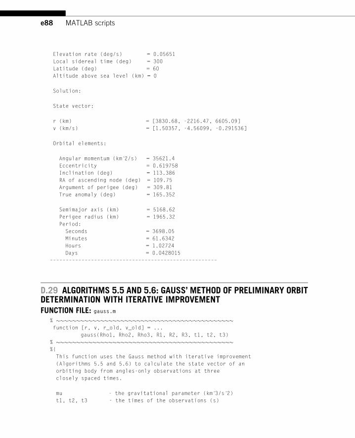
e88 MATLAB scripts
Elevation rate (deg/s) = 0.05651
Local sidereal time (deg) = 300
Latitude (deg) = 60
Altitude above sea level (km) = 0
Solution:
State vector:
r (km) = [3830.68, -2216.47, 6605.09]
v (km/s) = [1.50357, -4.56099, -0.291536]
Orbital elements:
Angular momentum (km 2̂/s) = 35621.4
Eccentricity = 0.619758
Inclination (deg) = 113.386
RA of ascending node (deg) = 109.75
Argument of perigee (deg) = 309.81
True anomaly (deg) = 165.352
Semimajor axis (km) = 5168.62
Perigee radius (km) = 1965.32
Period:
Seconds = 3698.05
Minutes = 61.6342
Hours = 1.02724
Days = 0.0428015
–––––––––––––––––––––––––––––––––––––––––––––––––––––
D.29 ALGORITHMS 5.5 AND 5.6: GAUSS’ METHOD OF PRELIMINARY ORBITDETERMINATION WITH ITERATIVE IMPROVEMENTFUNCTION FILE: gauss.m
% ��������������������������������������������function [r, v, r_old, v_old] = ...
gauss(Rho1, Rho2, Rho3, R1, R2, R3, t1, t2, t3)
% ��������������������������������������������%{
This function uses the Gauss method with iterative improvement
(Algorithms 5.5 and 5.6) to calculate the state vector of an
orbiting body from angles-only observations at three
closely spaced times.
mu - the gravitational parameter (km 3̂/s 2̂)
t1, t2, t3 - the times of the observations (s)
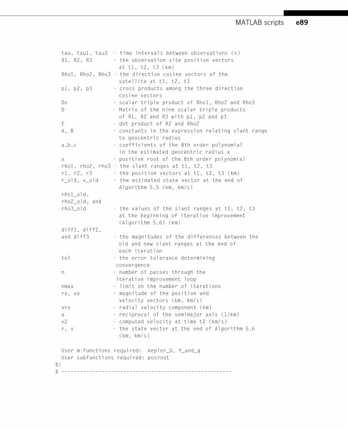
e89MATLAB scripts
tau, tau1, tau3 - time intervals between observations (s)
R1, R2, R3 - the observation site position vectors
at t1, t2, t3 (km)
Rho1, Rho2, Rho3 - the direction cosine vectors of the
satellite at t1, t2, t3
p1, p2, p3 - cross products among the three direction
cosine vectors
Do - scalar triple product of Rho1, Rho2 and Rho3
D - Matrix of the nine scalar triple products
of R1, R2 and R3 with p1, p2 and p3
E - dot product of R2 and Rho2
A, B - constants in the expression relating slant range
to geocentric radius
a,b,c - coefficients of the 8th order polynomial
in the estimated geocentric radius x
x - positive root of the 8th order polynomial
rho1, rho2, rho3 - the slant ranges at t1, t2, t3
r1, r2, r3 - the position vectors at t1, t2, t3 (km)
r_old, v_old - the estimated state vector at the end of
Algorithm 5.5 (km, km/s)
rho1_old,
rho2_old, and
rho3_old - the values of the slant ranges at t1, t2, t3
at the beginning of iterative improvement
(Algorithm 5.6) (km)
diff1, diff2,
and diff3 - the magnitudes of the differences between the
old and new slant ranges at the end of
each iteration
tol - the error tolerance determining
convergence
n - number of passes through the
iterative improvement loop
nmax - limit on the number of iterations
ro, vo - magnitude of the position and
velocity vectors (km, km/s)
vro - radial velocity component (km)
a - reciprocal of the semimajor axis (1/km)
v2 - computed velocity at time t2 (km/s)
r, v - the state vector at the end of Algorithm 5.6
(km, km/s)
User m-functions required: kepler_U, f_and_g
User subfunctions required: posroot
%}
% –––––––––––––––––––––––––––––––––––––––––––––––––––––––
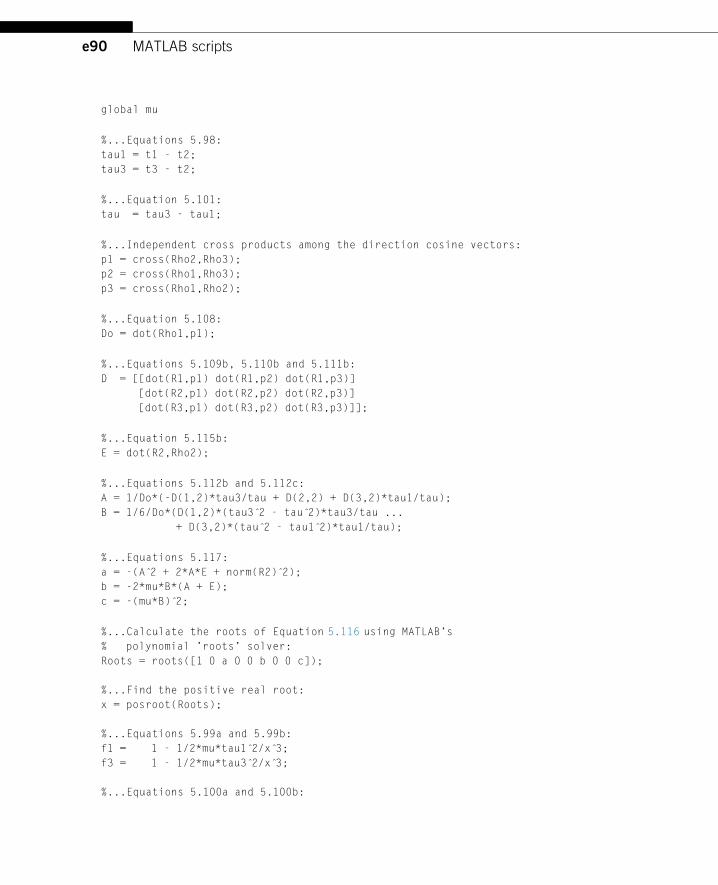
e90 MATLAB scripts
global mu
%...Equations 5.98:
tau1 = t1 - t2;
tau3 = t3 - t2;
%...Equation 5.101:
tau = tau3 - tau1;
%...Independent cross products among the direction cosine vectors:
p1 = cross(Rho2,Rho3);
p2 = cross(Rho1,Rho3);
p3 = cross(Rho1,Rho2);
%...Equation 5.108:
Do = dot(Rho1,p1);
%...Equations 5.109b, 5.110b and 5.111b:
D = [[dot(R1,p1) dot(R1,p2) dot(R1,p3)]
[dot(R2,p1) dot(R2,p2) dot(R2,p3)]
[dot(R3,p1) dot(R3,p2) dot(R3,p3)]];
%...Equation 5.115b:
E = dot(R2,Rho2);
%...Equations 5.112b and 5.112c:
A = 1/Do*(-D(1,2)*tau3/tau + D(2,2) + D(3,2)*tau1/tau);
B = 1/6/Do*(D(1,2)*(tau3 2̂ - tau 2̂)*tau3/tau ...
+ D(3,2)*(tau 2̂ - tau1 2̂)*tau1/tau);
%...Equations 5.117:
a = -(A 2̂ + 2*A*E + norm(R2) 2̂);
b = -2*mu*B*(A + E);
c = -(mu*B) 2̂;
%...Calculate the roots of Equation 5.116 using MATLAB’s
% polynomial ’roots’ solver:
Roots = roots([1 0 a 0 0 b 0 0 c]);
%...Find the positive real root:
x = posroot(Roots);
%...Equations 5.99a and 5.99b:
f1 = 1 - 1/2*mu*tau1 2̂/x 3̂;
f3 = 1 - 1/2*mu*tau3 2̂/x 3̂;
%...Equations 5.100a and 5.100b:
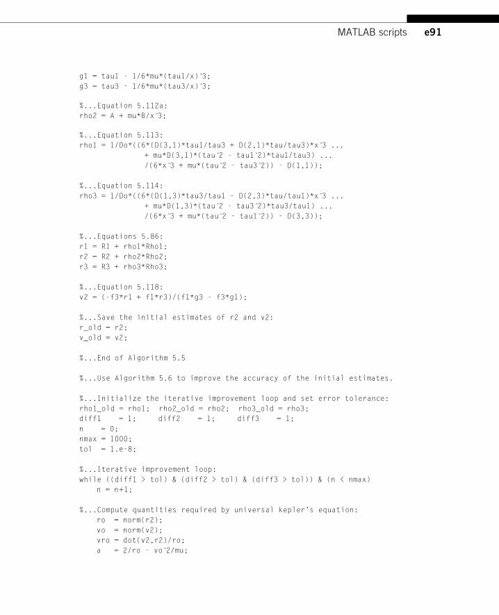
e91MATLAB scripts
g1 = tau1 - 1/6*mu*(tau1/x) 3̂;
g3 = tau3 - 1/6*mu*(tau3/x) 3̂;
%...Equation 5.112a:
rho2 = A + mu*B/x 3̂;
%...Equation 5.113:
rho1 = 1/Do*((6*(D(3,1)*tau1/tau3 + D(2,1)*tau/tau3)*x 3̂ ...
+ mu*D(3,1)*(tau 2̂ - tau1 2̂)*tau1/tau3) ...
/(6*x 3̂ + mu*(tau 2̂ - tau3 2̂)) - D(1,1));
%...Equation 5.114:
rho3 = 1/Do*((6*(D(1,3)*tau3/tau1 - D(2,3)*tau/tau1)*x 3̂ ...
+ mu*D(1,3)*(tau 2̂ - tau3 2̂)*tau3/tau1) ...
/(6*x 3̂ + mu*(tau 2̂ - tau1 2̂)) - D(3,3));
%...Equations 5.86:
r1 = R1 + rho1*Rho1;
r2 = R2 + rho2*Rho2;
r3 = R3 + rho3*Rho3;
%...Equation 5.118:
v2 = (-f3*r1 + f1*r3)/(f1*g3 - f3*g1);
%...Save the initial estimates of r2 and v2:
r_old = r2;
v_old = v2;
%...End of Algorithm 5.5
%...Use Algorithm 5.6 to improve the accuracy of the initial estimates.
%...Initialize the iterative improvement loop and set error tolerance:
rho1_old = rho1; rho2_old = rho2; rho3_old = rho3;
diff1 = 1; diff2 = 1; diff3 = 1;
n = 0;
nmax = 1000;
tol = 1.e-8;
%...Iterative improvement loop:
while ((diff1 > tol) & (diff2 > tol) & (diff3 > tol)) & (n < nmax)
n = n+1;
%...Compute quantities required by universal kepler’s equation:
ro = norm(r2);
vo = norm(v2);
vro = dot(v2,r2)/ro;
a = 2/ro - vo 2̂/mu;
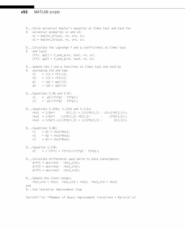
e92 MATLAB scripts
%...Solve universal Kepler’s equation at times tau1 and tau3 for
% universal anomalies x1 and x3:
x1 = kepler_U(tau1, ro, vro, a);
x3 = kepler_U(tau3, ro, vro, a);
%...Calculate the Lagrange f and g coefficients at times tau1
% and tau3:
[ff1, gg1] = f_and_g(x1, tau1, ro, a);
[ff3, gg3] = f_and_g(x3, tau3, ro, a);
%...Update the f and g functions at times tau1 and tau3 by
% averaging old and new:
f1 = (f1 + ff1)/2;
f3 = (f3 + ff3)/2;
g1 = (g1 + gg1)/2;
g3 = (g3 + gg3)/2;
%...Equations 5.96 and 5.97:
c1 = g3/(f1*g3 - f3*g1);
c3 = -g1/(f1*g3 - f3*g1);
%...Equations 5.109a, 5.110a and 5.111a:
rho1 = 1/Do*( -D(1,1) + 1/c1*D(2,1) - c3/c1*D(3,1));
rho2 = 1/Do*( -c1*D(1,2) +D(2,2) - c3*D(3,2));
rho3 = 1/Do*(-c1/c3*D(1,3) + 1/c3*D(2,3) - D(3,3));
%...Equations 5.86:
r1 = R1 + rho1*Rho1;
r2 = R2 + rho2*Rho2;
r3 = R3 + rho3*Rho3;
%...Equation 5.118:
v2 = (-f3*r1 + f1*r3)/(f1*g3 - f3*g1);
%...Calculate differences upon which to base convergence:
diff1 = abs(rho1 - rho1_old);
diff2 = abs(rho2 - rho2_old);
diff3 = abs(rho3 - rho3_old);
%...Update the slant ranges:
rho1_old = rho1; rho2_old = rho2; rho3_old = rho3;
end
%...End iterative improvement loop
fprintf(’\n( **Number of Gauss improvement iterations = %g)\n\n’,n)
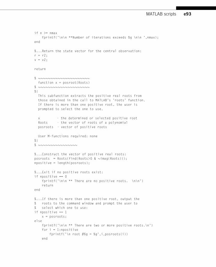
e93MATLAB scripts
if n >= nmax
fprintf(’\n\n **Number of iterations exceeds %g \n\n ’,nmax);
end
%...Return the state vector for the central observation:
r = r2;
v = v2;
return
% ���������������������function x = posroot(Roots)
% ���������������������%{
This subfunction extracts the positive real roots from
those obtained in the call to MATLAB’s ’roots’ function.
If there is more than one positive root, the user is
prompted to select the one to use.
x - the determined or selected positive root
Roots - the vector of roots of a polynomial
posroots - vector of positive roots
User M-functions required: none
%}
% ����������������
%...Construct the vector of positive real roots:
posroots = Roots(find(Roots>0 & �imag(Roots)));
npositive = length(posroots);
%...Exit if no positive roots exist:
if npositive == 0
fprintf(’\n\n ** There are no positive roots. \n\n’)
return
end
%...If there is more than one positive root, output the
% roots to the command window and prompt the user to
% select which one to use:
if npositive == 1
x = posroots;
else
fprintf(’\n\n ** There are two or more positive roots.\n’)
for i = 1:npositive
fprintf(’\n root #%g = %g’,i,posroots(i))
end
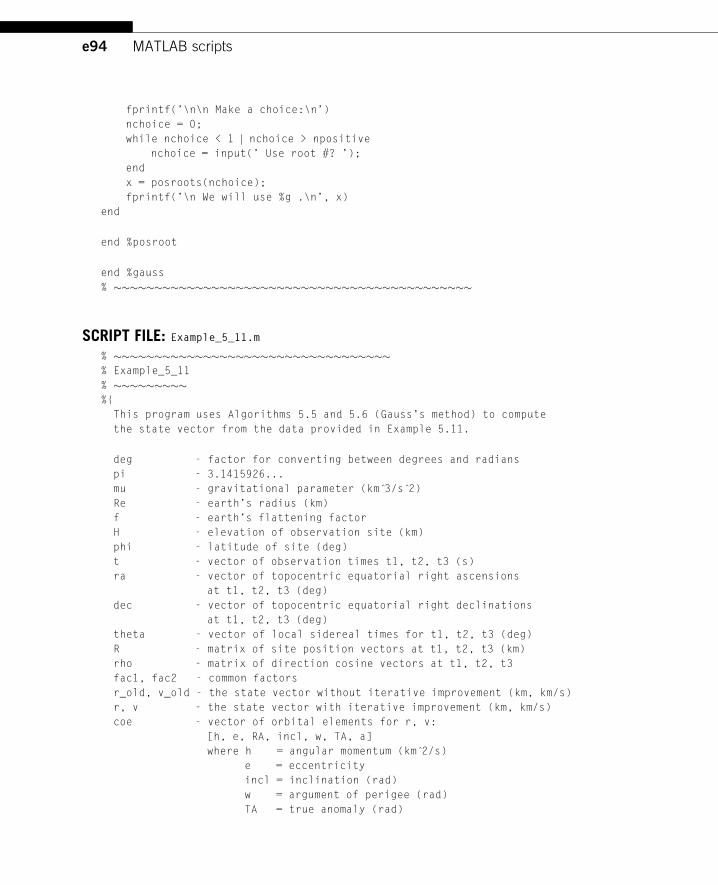
e94 MATLAB scripts
fprintf(’\n\n Make a choice:\n’)
nchoice = 0;
while nchoice < 1 j nchoice > npositive
nchoice = input(’ Use root #? ’);
end
x = posroots(nchoice);
fprintf(’\n We will use %g .\n’, x)
end
end %posroot
end %gauss
% ��������������������������������������������
SCRIPT FILE: Example_5_11.m
% ����������������������������������% Example_5_11
% ���������%{
This program uses Algorithms 5.5 and 5.6 (Gauss’s method) to compute
the state vector from the data provided in Example 5.11.
deg - factor for converting between degrees and radians
pi - 3.1415926...
mu - gravitational parameter (km 3̂/s 2̂)
Re - earth’s radius (km)
f - earth’s flattening factor
H - elevation of observation site (km)
phi - latitude of site (deg)
t - vector of observation times t1, t2, t3 (s)
ra - vector of topocentric equatorial right ascensions
at t1, t2, t3 (deg)
dec - vector of topocentric equatorial right declinations
at t1, t2, t3 (deg)
theta - vector of local sidereal times for t1, t2, t3 (deg)
R - matrix of site position vectors at t1, t2, t3 (km)
rho - matrix of direction cosine vectors at t1, t2, t3
fac1, fac2 - common factors
r_old, v_old - the state vector without iterative improvement (km, km/s)
r, v - the state vector with iterative improvement (km, km/s)
coe - vector of orbital elements for r, v:
[h, e, RA, incl, w, TA, a]
where h = angular momentum (km 2̂/s)
e = eccentricity
incl = inclination (rad)
w = argument of perigee (rad)
TA = true anomaly (rad)
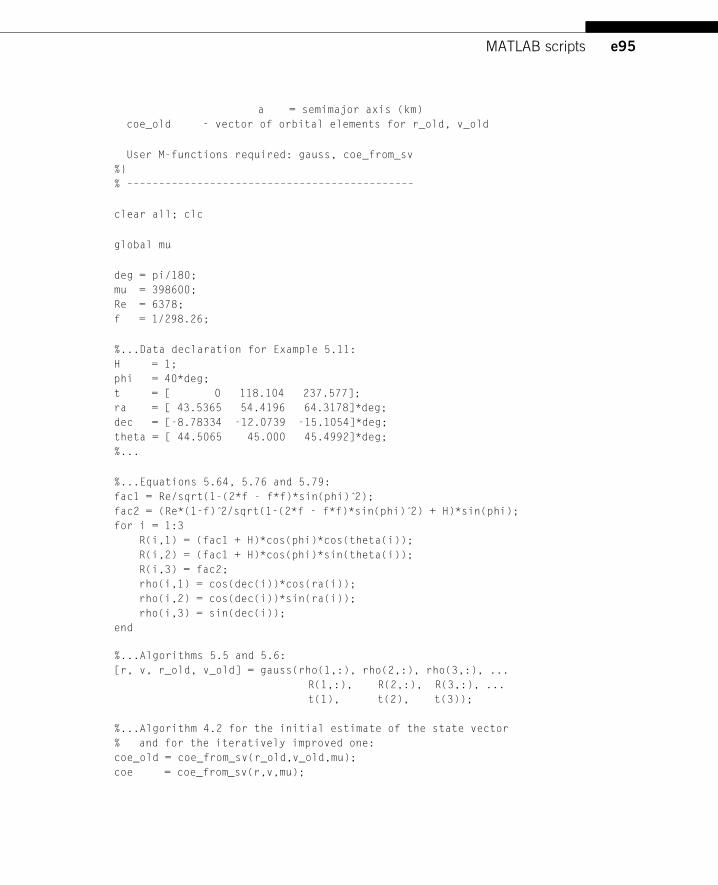
e95MATLAB scripts
a = semimajor axis (km)
coe_old - vector of orbital elements for r_old, v_old
User M-functions required: gauss, coe_from_sv
%}
% –––––––––––––––––––––––––––––––––––––––––––––
clear all; clc
global mu
deg = pi/180;
mu = 398600;
Re = 6378;
f = 1/298.26;
%...Data declaration for Example 5.11:
H = 1;
phi = 40*deg;
t = [ 0 118.104 237.577];
ra = [ 43.5365 54.4196 64.3178]*deg;
dec = [-8.78334 -12.0739 -15.1054]*deg;
theta = [ 44.5065 45.000 45.4992]*deg;
%...
%...Equations 5.64, 5.76 and 5.79:
fac1 = Re/sqrt(1-(2*f - f*f)*sin(phi) 2̂);
fac2 = (Re*(1-f) 2̂/sqrt(1-(2*f - f*f)*sin(phi) 2̂) + H)*sin(phi);
for i = 1:3
R(i,1) = (fac1 + H)*cos(phi)*cos(theta(i));
R(i,2) = (fac1 + H)*cos(phi)*sin(theta(i));
R(i,3) = fac2;
rho(i,1) = cos(dec(i))*cos(ra(i));
rho(i,2) = cos(dec(i))*sin(ra(i));
rho(i,3) = sin(dec(i));
end
%...Algorithms 5.5 and 5.6:
[r, v, r_old, v_old] = gauss(rho(1,:), rho(2,:), rho(3,:), ...
R(1,:), R(2,:), R(3,:), ...
t(1), t(2), t(3));
%...Algorithm 4.2 for the initial estimate of the state vector
% and for the iteratively improved one:
coe_old = coe_from_sv(r_old,v_old,mu);
coe = coe_from_sv(r,v,mu);
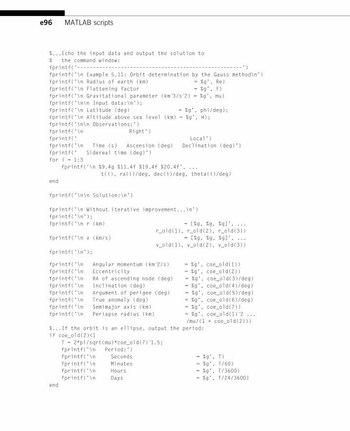
e96 MATLAB scripts
%...Echo the input data and output the solution to
% the command window:
fprintf(’–––––––––––––––––––––––––––––––––––––––––––––––––––––’)
fprintf(’\n Example 5.11: Orbit determination by the Gauss method\n’)
fprintf(’\n Radius of earth (km) = %g’, Re)
fprintf(’\n Flattening factor = %g’, f)
fprintf(’\n Gravitational parameter (km 3̂/s 2̂) = %g’, mu)
fprintf(’\n\n Input data:\n’);
fprintf(’\n Latitude (deg) = %g’, phi/deg);
fprintf(’\n Altitude above sea level (km) = %g’, H);
fprintf(’\n\n Observations:’)
fprintf(’\n Right’)
fprintf(’ Local’)
fprintf(’\n Time (s) Ascension (deg) Declination (deg)’)
fprintf(’ Sidereal time (deg)’)
for i = 1:3
fprintf(’\n %9.4g %11.4f %19.4f %20.4f’, ...
t(i), ra(i)/deg, dec(i)/deg, theta(i)/deg)
end
fprintf(’\n\n Solution:\n’)
fprintf(’\n Without iterative improvement...\n’)
fprintf(’\n’);
fprintf(’\n r (km) = [%g, %g, %g]’, ...
r_old(1), r_old(2), r_old(3))
fprintf(’\n v (km/s) = [%g, %g, %g]’, ...
v_old(1), v_old(2), v_old(3))
fprintf(’\n’);
fprintf(’\n Angular momentum (km 2̂/s) = %g’, coe_old(1))
fprintf(’\n Eccentricity = %g’, coe_old(2))
fprintf(’\n RA of ascending node (deg) = %g’, coe_old(3)/deg)
fprintf(’\n Inclination (deg) = %g’, coe_old(4)/deg)
fprintf(’\n Argument of perigee (deg) = %g’, coe_old(5)/deg)
fprintf(’\n True anomaly (deg) = %g’, coe_old(6)/deg)
fprintf(’\n Semimajor axis (km) = %g’, coe_old(7))
fprintf(’\n Periapse radius (km) = %g’, coe_old(1) 2̂ ...
/mu/(1 + coe_old(2)))
%...If the orbit is an ellipse, output the period:
if coe_old(2)<1
T = 2*pi/sqrt(mu)*coe_old(7) 1̂.5;
fprintf(’\n Period:’)
fprintf(’\n Seconds = %g’, T)
fprintf(’\n Minutes = %g’, T/60)
fprintf(’\n Hours = %g’, T/3600)
fprintf(’\n Days = %g’, T/24/3600)
end
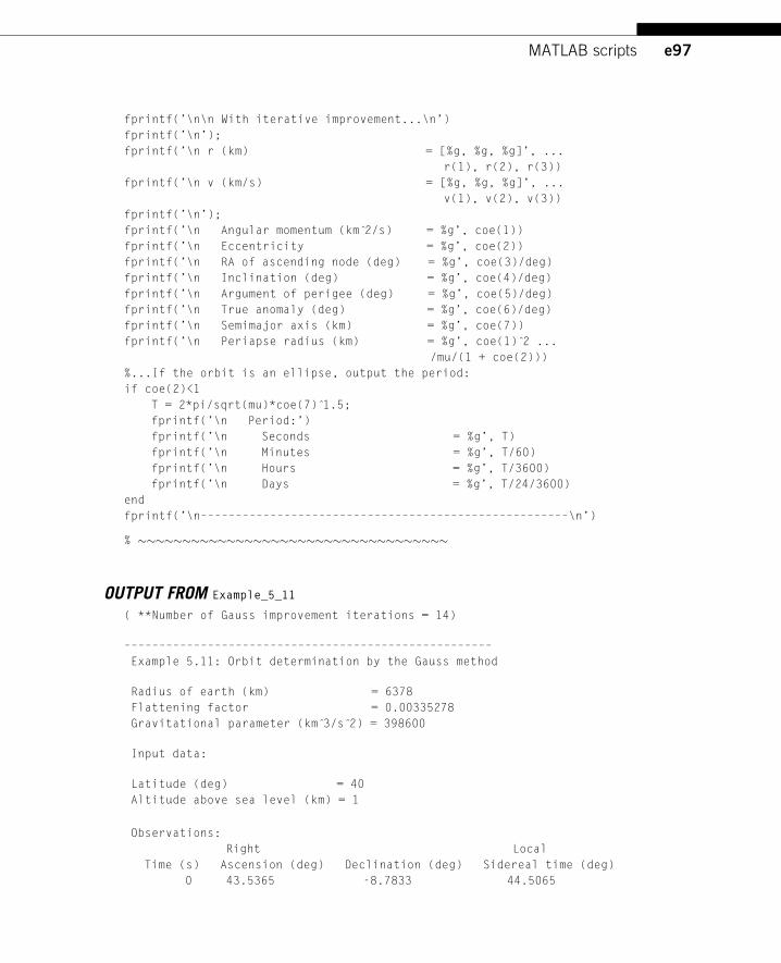
e97MATLAB scripts
fprintf(’\n\n With iterative improvement...\n’)
fprintf(’\n’);
fprintf(’\n r (km) = [%g, %g, %g]’, ...
r(1), r(2), r(3))
fprintf(’\n v (km/s) = [%g, %g, %g]’, ...
v(1), v(2), v(3))
fprintf(’\n’);
fprintf(’\n Angular momentum (km 2̂/s) = %g’, coe(1))
fprintf(’\n Eccentricity = %g’, coe(2))
fprintf(’\n RA of ascending node (deg) = %g’, coe(3)/deg)
fprintf(’\n Inclination (deg) = %g’, coe(4)/deg)
fprintf(’\n Argument of perigee (deg) = %g’, coe(5)/deg)
fprintf(’\n True anomaly (deg) = %g’, coe(6)/deg)
fprintf(’\n Semimajor axis (km) = %g’, coe(7))
fprintf(’\n Periapse radius (km) = %g’, coe(1) 2̂ ...
/mu/(1 + coe(2)))
%...If the orbit is an ellipse, output the period:
if coe(2)<1
T = 2*pi/sqrt(mu)*coe(7) 1̂.5;
fprintf(’\n Period:’)
fprintf(’\n Seconds = %g’, T)
fprintf(’\n Minutes = %g’, T/60)
fprintf(’\n Hours = %g’, T/3600)
fprintf(’\n Days = %g’, T/24/3600)
end
fprintf(’\n–––––––––––––––––––––––––––––––––––––––––––––––––––––\n’)
% �����������������������������������
OUTPUT FROM Example_5_11
( **Number of Gauss improvement iterations = 14)
–––––––––––––––––––––––––––––––––––––––––––––––––––––
Example 5.11: Orbit determination by the Gauss method
Radius of earth (km) = 6378
Flattening factor = 0.00335278
Gravitational parameter (km 3̂/s 2̂) = 398600
Input data:
Latitude (deg) = 40
Altitude above sea level (km) = 1
Observations:
Right Local
Time (s) Ascension (deg) Declination (deg) Sidereal time (deg)
0 43.5365 -8.7833 44.5065
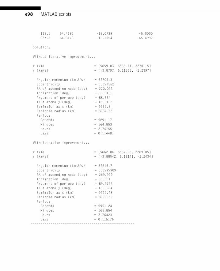
e98 MATLAB scripts
118.1 54.4196 -12.0739 45.0000
237.6 64.3178 -15.1054 45.4992
Solution:
Without iterative improvement...
r (km) = [5659.03, 6533.74, 3270.15]
v (km/s) = [-3.8797, 5.11565, -2.2397]
Angular momentum (km 2̂/s) = 62705.3
Eccentricity = 0.097562
RA of ascending node (deg) = 270.023
Inclination (deg) = 30.0105
Argument of perigee (deg) = 88.654
True anomaly (deg) = 46.3163
Semimajor axis (km) = 9959.2
Periapse radius (km) = 8987.56
Period:
Seconds = 9891.17
Minutes = 164.853
Hours = 2.74755
Days = 0.114481
With iterative improvement...
r (km) = [5662.04, 6537.95, 3269.05]
v (km/s) = [-3.88542, 5.12141, -2.2434]
Angular momentum (km 2̂/s) = 62816.7
Eccentricity = 0.0999909
RA of ascending node (deg) = 269.999
Inclination (deg) = 30.001
Argument of perigee (deg) = 89.9723
True anomaly (deg) = 45.0284
Semimajor axis (km) = 9999.48
Periapse radius (km) = 8999.62
Period:
Seconds = 9951.24
Minutes = 165.854
Hours = 2.76423
Days = 0.115176
–––––––––––––––––––––––––––––––––––––––––––––––––––––
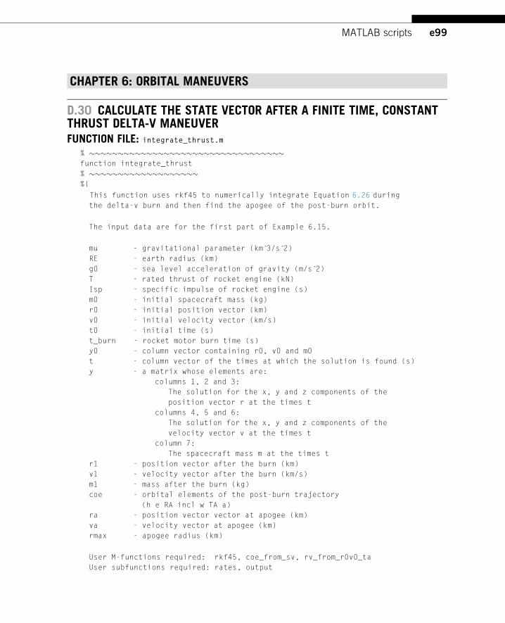
e99MATLAB scripts
CHAPTER 6: ORBITAL MANEUVERS
D.30 CALCULATE THE STATE VECTOR AFTER A FINITE TIME, CONSTANTTHRUST DELTA-V MANEUVERFUNCTION FILE: integrate_thrust.m
% ����������������������������������function integrate_thrust
% �������������������%{
This function uses rkf45 to numerically integrate Equation 6.26 during
the delta-v burn and then find the apogee of the post-burn orbit.
The input data are for the first part of Example 6.15.
mu - gravitational parameter (km 3̂/s 2̂)
RE - earth radius (km)
g0 - sea level acceleration of gravity (m/s 2̂)
T - rated thrust of rocket engine (kN)
Isp - specific impulse of rocket engine (s)
m0 - initial spacecraft mass (kg)
r0 - initial position vector (km)
v0 - initial velocity vector (km/s)
t0 - initial time (s)
t_burn - rocket motor burn time (s)
y0 - column vector containing r0, v0 and m0
t - column vector of the times at which the solution is found (s)
y - a matrix whose elements are:
columns 1, 2 and 3:
The solution for the x, y and z components of the
position vector r at the times t
columns 4, 5 and 6:
The solution for the x, y and z components of the
velocity vector v at the times t
column 7:
The spacecraft mass m at the times t
r1 - position vector after the burn (km)
v1 - velocity vector after the burn (km/s)
m1 - mass after the burn (kg)
coe - orbital elements of the post-burn trajectory
(h e RA incl w TA a)
ra - position vector vector at apogee (km)
va - velocity vector at apogee (km)
rmax - apogee radius (km)
User M-functions required: rkf45, coe_from_sv, rv_from_r0v0_ta
User subfunctions required: rates, output
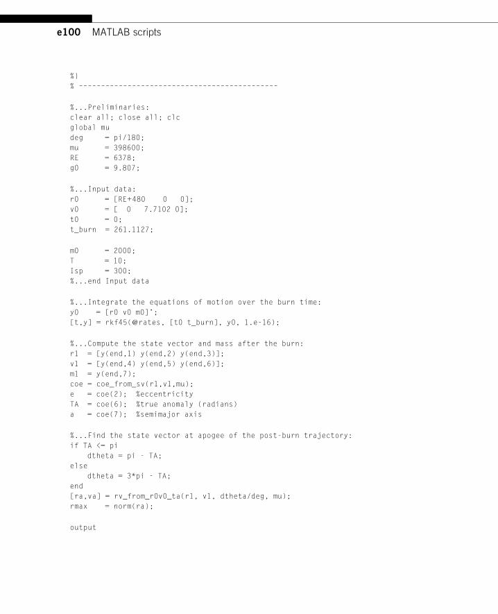
e100 MATLAB scripts
%}
% –––––––––––––––––––––––––––––––––––––––––––––
%...Preliminaries:
clear all; close all; clc
global mu
deg = pi/180;
mu = 398600;
RE = 6378;
g0 = 9.807;
%...Input data:
r0 = [RE+480 0 0];
v0 = [ 0 7.7102 0];
t0 = 0;
t_burn = 261.1127;
m0 = 2000;
T = 10;
Isp = 300;
%...end Input data
%...Integrate the equations of motion over the burn time:
y0 = [r0 v0 m0]’;
[t,y] = rkf45(@rates, [t0 t_burn], y0, 1.e-16);
%...Compute the state vector and mass after the burn:
r1 = [y(end,1) y(end,2) y(end,3)];
v1 = [y(end,4) y(end,5) y(end,6)];
m1 = y(end,7);
coe = coe_from_sv(r1,v1,mu);
e = coe(2); %eccentricity
TA = coe(6); %true anomaly (radians)
a = coe(7); %semimajor axis
%...Find the state vector at apogee of the post-burn trajectory:
if TA <= pi
dtheta = pi - TA;
else
dtheta = 3*pi - TA;
end
[ra,va] = rv_from_r0v0_ta(r1, v1, dtheta/deg, mu);
rmax = norm(ra);
output
e101MATLAB scripts
%...Subfunctions:
% �������������������function dfdt = rates(t,f)
% �������������������%{
This function calculates the acceleration vector using Equation 6.26.
t - time (s)
f - column vector containing the position vector, velocity
vector and the mass at time t
x, y, z - components of the position vector (km)
vx, vy, vz - components of the velocity vector (km/s)
m - mass (kg)
r - magnitude of the the position vector (km)
v - magnitude of the velocity vector (km/s)
ax, ay, az - components of the acceleration vector (km/s 2̂)
mdot - rate of change of mass (kg/s)
dfdt - column vector containing the velocity and acceleration
components and the mass rate
%}
% ––––––––––––––––––––––––
x = f(1); y = f(2); z = f(3);
vx = f(4); vy = f(5); vz = f(6);
m = f(7);
r = norm([x y z]);
v = norm([vx vy vz]);
ax = -mu*x/r 3̂ + T/m*vx/v;
ay = -mu*y/r 3̂ + T/m*vy/v;
az = -mu*z/r 3̂ + T/m*vz/v;
mdot = -T*1000/g0/Isp;
dfdt = [vx vy vz ax ay az mdot]’;
end %rates
% ����������function output
% ����������fprintf(’\n\n––––––––––––––––––––––––––––––––––––––--–––––––––––––––––\n’)
fprintf(’\nBefore ignition:’)
fprintf(’\n Mass = %g kg’, m0)
fprintf(’\n State vector:’)
fprintf(’\n r = [%10g, %10g, %10g] (km)’, r0(1), r0(2), r0(3))
fprintf(’\n Radius = %g’, norm(r0))
fprintf(’\n v = [%10g, %10g, %10g] (km/s)’, v0(1), v0(2), v0(3))
e102 MATLAB scripts
fprintf(’\n Speed = %g\n’, norm(v0))
fprintf(’\nThrust = %12g kN’, T)
fprintf(’\nBurn time = %12.6f s’, t_burn)
fprintf(’\nMass after burn = %12.6E kg\n’, m1)
fprintf(’\nEnd-of-burn-state vector:’)
fprintf(’\n r = [%10g, %10g, %10g] (km)’, r1(1), r1(2), r1(3))
fprintf(’\n Radius = %g’, norm(r1))
fprintf(’\n v = [%10g, %10g, %10g] (km/s)’, v1(1), v1(2), v1(3))
fprintf(’\n Speed = %g\n’, norm(v1))
fprintf(’\nPost-burn trajectory:’)
fprintf(’\n Eccentricity = %g’, e)
fprintf(’\n Semimajor axis = %g km’, a)
fprintf(’\n Apogee state vector:’)
fprintf(’\n r = [%17.10E, %17.10E, %17.10E] (km)’, ra(1), ra(2), ra(3))
fprintf(’\n Radius = %g’, norm(ra))
fprintf(’\n v = [%17.10E, %17.10E, %17.10E] (km/s)’, va(1), va(2), va(3))
fprintf(’\n Speed = %g’, norm(va))
fprintf(’\n\n––––––––––––––––––––––––––––––––––––––--–––––––––––––––––\n\n’)
end %output
end %integrate_thrust
CHAPTER 7: RELATIVE MOTION AND RENDEZVOUS
D.31 ALGORITHM 7.1: FIND THE POSITION, VELOCITY, AND ACCELERATIONOF B RELATIVE TO A’S LVLH FRAMEFUNCTION FILE: rva_relative.m
% ��������������������������������������������������function [r_rel_x, v_rel_x, a_rel_x] = rva_relative(rA,vA,rB,vB)
% ��������������������������������������������������%{
This function uses the state vectors of spacecraft A and B
to find the position, velocity and acceleration of B relative
to A in the LVLH frame attached to A (see Figure 7.1).
rA,vA - state vector of A (km, km/s)
rB,vB - state vector of B (km, km/s)
mu - gravitational parameter (km 3̂/s 2̂)
hA - angular momentum vector of A (km 2̂/s)
i, j, k - unit vectors along the x, y and z axes of A’s
LVLH frame
QXx - DCM of the LVLH frame relative to the geocentric
equatorial frame (GEF)
Omega - angular velocity of the LVLH frame (rad/s)
e103MATLAB scripts
Omega_dot - angular acceleration of the LVLH frame (rad/s 2̂)
aA, aB - absolute accelerations of A and B (km/s 2̂)
r_rel - position of B relative to A in GEF (km)
v_rel - velocity of B relative to A in GEF (km/s)
a_rel - acceleration of B relative to A in GEF (km/s 2̂)
r_rel_x - position of B relative to A in the LVLH frame
v_rel_x - velocity of B relative to A in the LVLH frame
a_rel_x - acceleration of B relative to A in the LVLH frame
User M-functions required: None
%}
% –––––––––––––––––––––––––––––––––––––––––––––––––––––––––––
global mu
%...Calculate the vector hA:
hA = cross(rA, vA);
%...Calculate the unit vectors i, j and k:
i = rA/norm(rA);
k = hA/norm(hA);
j = cross(k,i);
%...Calculate the transformation matrix Qxx:
QXx = [i; j; k];
%...Calculate Omega and Omega_dot:
Omega = hA/norm(rA) 2̂; % Equation 7.5
Omega_dot = -2*dot(rA,vA)/norm(rA) 2̂*Omega;% Equation 7.6
%...Calculate the accelerations aA and aB:
aA = -mu*rA/norm(rA) 3̂;
aB = -mu*rB/norm(rB) 3̂;
%...Calculate r_rel:
r_rel = rB - rA;
%...Calculate v_rel:
v_rel = vB - vA - cross(Omega,r_rel);
%...Calculate a_rel:
a_rel = aB - aA - cross(Omega_dot,r_rel)...
- cross(Omega,cross(Omega,r_rel))...
- 2*cross(Omega,v_rel);
%...Calculate r_rel_x, v_rel_x and a_rel_x:
r_rel_x = QXx*r_rel’;
e104 MATLAB scripts
v_rel_x = QXx*v_rel’;
a_rel_x = QXx*a_rel’;
end %rva_relative
% ��������������������������������������������������
SCRIPT FILE: Example_7_01.m
% ��������������������������������������������������% Example_7_01
% ����������%{
This program uses the data of Example 7.1 to calculate the position,
velocity and acceleration of an orbiting chaser B relative to an
orbiting target A.
mu - gravitational parameter (km 3̂/s 2̂)
deg - conversion factor from degrees to radians
Spacecraft A & B:
h_A, h_B - angular momentum (km 2̂/s)
e_A, E_B - eccentricity
i_A, i_B - inclination (radians)
RAAN_A, RAAN_B - right ascension of the ascending node (radians)
omega_A, omega_B - argument of perigee (radians)
theta_A, theta_A - true anomaly (radians)
rA, vA - inertial position (km) and velocity (km/s) of A
rB, vB - inertial position (km) and velocity (km/s) of B
r - position (km) of B relative to A in A’s
co-moving frame
v - velocity (km/s) of B relative to A in A’s
co-moving frame
a - acceleration (km/s 2̂) of B relative to A in A’s
co-moving frame
User M-function required: sv_from_coe, rva_relative
User subfunctions required: none
%}
% –––––––––––––––––––––––––––––––––––––––––––––––––––––––––––
clear all; clc
global mu
mu = 398600;
deg = pi/180;
%...Input data:
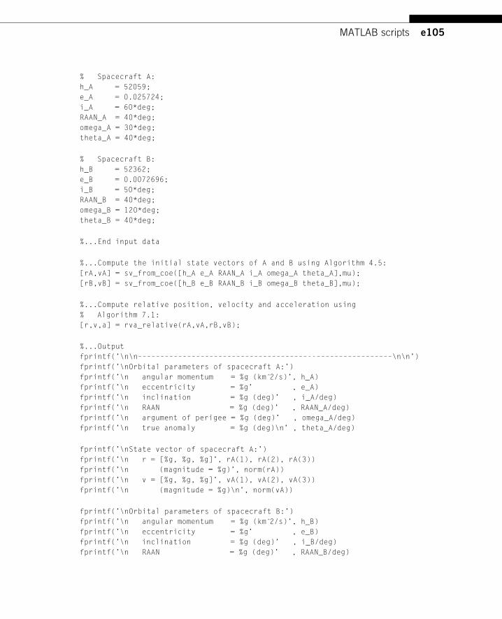
e105MATLAB scripts
% Spacecraft A:
h_A = 52059;
e_A = 0.025724;
i_A = 60*deg;
RAAN_A = 40*deg;
omega_A = 30*deg;
theta_A = 40*deg;
% Spacecraft B:
h_B = 52362;
e_B = 0.0072696;
i_B = 50*deg;
RAAN_B = 40*deg;
omega_B = 120*deg;
theta_B = 40*deg;
%...End input data
%...Compute the initial state vectors of A and B using Algorithm 4.5:
[rA,vA] = sv_from_coe([h_A e_A RAAN_A i_A omega_A theta_A],mu);
[rB,vB] = sv_from_coe([h_B e_B RAAN_B i_B omega_B theta_B],mu);
%...Compute relative position, velocity and acceleration using
% Algorithm 7.1:
[r,v,a] = rva_relative(rA,vA,rB,vB);
%...Output
fprintf(’\n\n––––––––––––––––––––––––––––––––––––––--–––––––––––––––––\n\n’)
fprintf(’\nOrbital parameters of spacecraft A:’)
fprintf(’\n angular momentum = %g (km 2̂/s)’, h_A)
fprintf(’\n eccentricity = %g’ , e_A)
fprintf(’\n inclination = %g (deg)’ , i_A/deg)
fprintf(’\n RAAN = %g (deg)’ , RAAN_A/deg)
fprintf(’\n argument of perigee = %g (deg)’ , omega_A/deg)
fprintf(’\n true anomaly = %g (deg)\n’ , theta_A/deg)
fprintf(’\nState vector of spacecraft A:’)
fprintf(’\n r = [%g, %g, %g]’, rA(1), rA(2), rA(3))
fprintf(’\n (magnitude = %g)’, norm(rA))
fprintf(’\n v = [%g, %g, %g]’, vA(1), vA(2), vA(3))
fprintf(’\n (magnitude = %g)\n’, norm(vA))
fprintf(’\nOrbital parameters of spacecraft B:’)
fprintf(’\n angular momentum = %g (km 2̂/s)’, h_B)
fprintf(’\n eccentricity = %g’ , e_B)
fprintf(’\n inclination = %g (deg)’ , i_B/deg)
fprintf(’\n RAAN = %g (deg)’ , RAAN_B/deg)
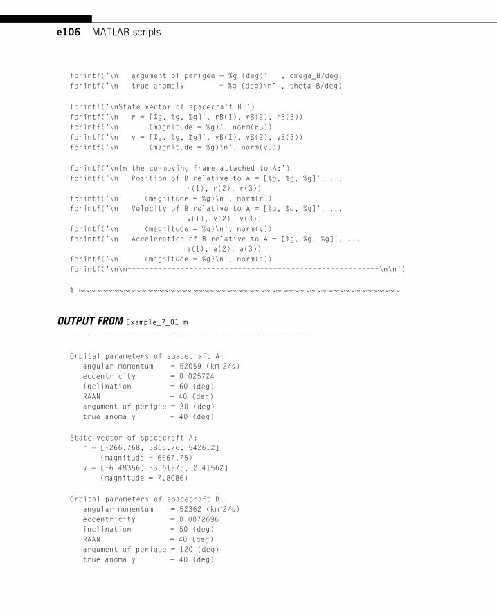
e106 MATLAB scripts
fprintf(’\n argument of perigee = %g (deg)’ , omega_B/deg)
fprintf(’\n true anomaly = %g (deg)\n’ , theta_B/deg)
fprintf(’\nState vector of spacecraft B:’)
fprintf(’\n r = [%g, %g, %g]’, rB(1), rB(2), rB(3))
fprintf(’\n (magnitude = %g)’, norm(rB))
fprintf(’\n v = [%g, %g, %g]’, vB(1), vB(2), vB(3))
fprintf(’\n (magnitude = %g)\n’, norm(vB))
fprintf(’\nIn the co-moving frame attached to A:’)
fprintf(’\n Position of B relative to A = [%g, %g, %g]’, ...
r(1), r(2), r(3))
fprintf(’\n (magnitude = %g)\n’, norm(r))
fprintf(’\n Velocity of B relative to A = [%g, %g, %g]’, ...
v(1), v(2), v(3))
fprintf(’\n (magnitude = %g)\n’, norm(v))
fprintf(’\n Acceleration of B relative to A = [%g, %g, %g]’, ...
a(1), a(2), a(3))
fprintf(’\n (magnitude = %g)\n’, norm(a))
fprintf(’\n\n––––––––––––––––––––––––––––––––––––––--–––––––––––––––––\n\n’)
% ���������������������������������������������������������
OUTPUT FROM Example_7_01.m
––––––––––––––––––––––––––––––––––––––––––––––––––––––––
Orbital parameters of spacecraft A:
angular momentum = 52059 (km 2̂/s)
eccentricity = 0.025724
inclination = 60 (deg)
RAAN = 40 (deg)
argument of perigee = 30 (deg)
true anomaly = 40 (deg)
State vector of spacecraft A:
r = [-266.768, 3865.76, 5426.2]
(magnitude = 6667.75)
v = [-6.48356, -3.61975, 2.41562]
(magnitude = 7.8086)
Orbital parameters of spacecraft B:
angular momentum = 52362 (km 2̂/s)
eccentricity = 0.0072696
inclination = 50 (deg)
RAAN = 40 (deg)
argument of perigee = 120 (deg)
true anomaly = 40 (deg)
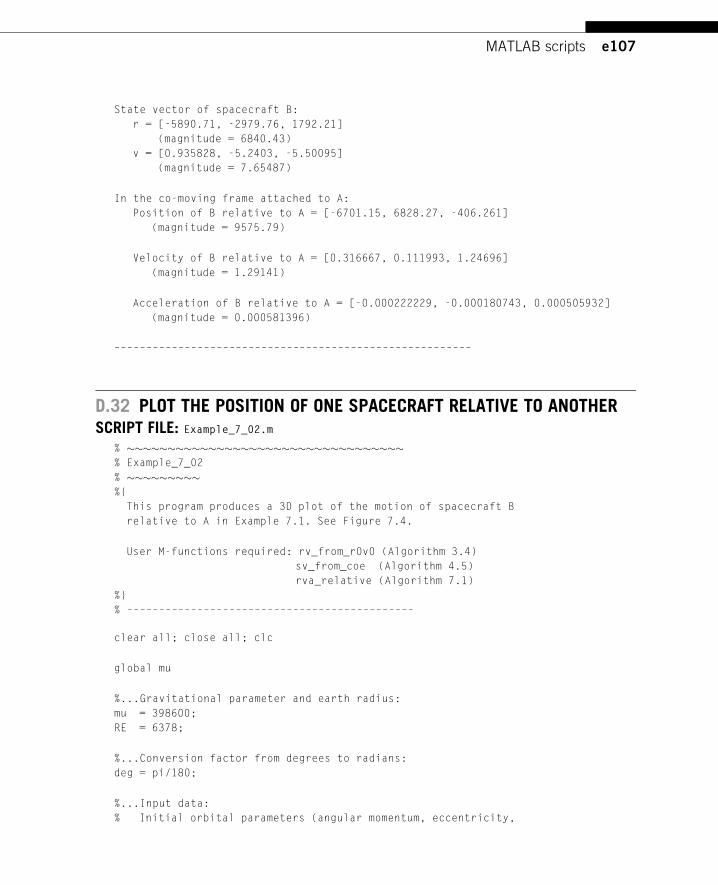
e107MATLAB scripts
State vector of spacecraft B:
r = [-5890.71, -2979.76, 1792.21]
(magnitude = 6840.43)
v = [0.935828, -5.2403, -5.50095]
(magnitude = 7.65487)
In the co-moving frame attached to A:
Position of B relative to A = [-6701.15, 6828.27, -406.261]
(magnitude = 9575.79)
Velocity of B relative to A = [0.316667, 0.111993, 1.24696]
(magnitude = 1.29141)
Acceleration of B relative to A = [-0.000222229, -0.000180743, 0.000505932]
(magnitude = 0.000581396)
––––––––––––––––––––––––––––––––––––––––––––––––––––––––
D.32 PLOT THE POSITION OF ONE SPACECRAFT RELATIVE TO ANOTHERSCRIPT FILE: Example_7_02.m
% ����������������������������������% Example_7_02
% ���������%{
This program produces a 3D plot of the motion of spacecraft B
relative to A in Example 7.1. See Figure 7.4.
User M-functions required: rv_from_r0v0 (Algorithm 3.4)
sv_from_coe (Algorithm 4.5)
rva_relative (Algorithm 7.1)
%}
% –––––––––––––––––––––––––––––––––––––––––––––
clear all; close all; clc
global mu
%...Gravitational parameter and earth radius:
mu = 398600;
RE = 6378;
%...Conversion factor from degrees to radians:
deg = pi/180;
%...Input data:
% Initial orbital parameters (angular momentum, eccentricity,
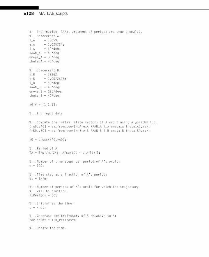
e108 MATLAB scripts
% inclination, RAAN, argument of perigee and true anomaly).
% Spacecraft A:
h_A = 52059;
e_A = 0.025724;
i_A = 60*deg;
RAAN_A = 40*deg;
omega_A = 30*deg;
theta_A = 40*deg;
% Spacecraft B:
h_B = 52362;
e_B = 0.0072696;
i_B = 50*deg;
RAAN_B = 40*deg;
omega_B = 120*deg;
theta_B = 40*deg;
vdir = [1 1 1];
%...End input data
%...Compute the initial state vectors of A and B using Algorithm 4.5:
[rA0,vA0] = sv_from_coe([h_A e_A RAAN_A i_A omega_A theta_A],mu);
[rB0,vB0] = sv_from_coe([h_B e_B RAAN_B i_B omega_B theta_B],mu);
h0 = cross(rA0,vA0);
%...Period of A:
TA = 2*pi/mu 2̂*(h_A/sqrt(1 - e_A 2̂)) 3̂;
%...Number of time steps per period of A’s orbit:
n = 100;
%...Time step as a fraction of A’s period:
dt = TA/n;
%...Number of periods of A’s orbit for which the trajectory
% will be plotted:
n_Periods = 60;
%...Initialize the time:
t = - dt;
%...Generate the trajectory of B relative to A:
for count = 1:n_Periods*n
%...Update the time:
e109MATLAB scripts
t = t + dt;
%...Update the state vector of both orbits using Algorithm 3.4:
[rA,vA] = rv_from_r0v0(rA0, vA0, t);
[rB,vB] = rv_from_r0v0(rB0, vB0, t);
%...Compute r_rel using Algorithm 7.1:
[r_rel, v_rel, a_rel] = rva_relative(rA,vA,rB,vB);
%...Store the components of the relative position vector
% at this time step in the vectors x, y and z, respectively:
x(count) = r_rel(1);
y(count) = r_rel(2);
z(count) = r_rel(3);
r(count) = norm(r_rel);
T(count) = t;
end
%...Plot the trajectory of B relative to A:
figure(1)
plot3(x, y, z)
hold on
axis equal
axis on
grid on
box off
view(vdir)
% Draw the co-moving x, y and z axes:
line([0 4000], [0 0], [0 0]); text(4000, 0, 0, ’x’)
line( [0 0], [0 7000], [0 0]); text( 0, 7000, 0, ’y’)
line( [0 0], [0 0], [0 4000]); text( 0, 0, 4000, ’z’)
% Label the origin of the moving frame attached to A:
text (0, 0, 0, ’A’)
% Label the start of B’s relative trajectory:
text(x(1), y(1), z(1), ’B’)
% Draw the initial position vector of B:
line([0 x(1)], [0 y(1)], [0 z(1)])
% ����������������������������������
e110 MATLAB scripts
D.33 SOLUTION OF THE LINEARIZED EQUATIONS OF RELATIVE MOTIONWITH AN ELLIPTICAL REFERENCE ORBITFUNCTION FILE: Example_7_03.m
% ����������������������������������function Example_7_03
% ���������������%{
This function plots the motion of chaser B relative to target A
for the data in Example 7.3. See Figures 7.6 and 7.7.
mu - gravitational parameter (km 3̂/s 2̂)
RE - radius of the earth (km)
Target orbit at time t = 0:
rp - perigee radius (km)
e - eccentricity
i - inclination (rad)
RA - right ascension of the ascending node (rad)
omega - argument of perigee (rad)
theta - true anomaly (rad)
ra - apogee radius (km)
h - angular momentum (km 2̂/s)
a - semimajor axis (km)
T - period (s)
n - mean motion (rad/s)
dr0, dv0 - initial relative position (km) and relative velocity (km/s)
of B in the co-moving frame
t0, tf - initial and final times (s) for the numerical integration
R0, V0 - initial position (km) and velocity (km/s) of A in the
geocentric equatorial frame
y0 - column vector containing r0, v0
%}
% User M-functions required: sv_from_coe, rkf45
% User subfunctions required: rates
% –––––––––––––––––––––––––––––––––––––––––––––
clear all; close all; clc
global mu
mu = 398600;
RE = 6378;
%...Input data:
% Prescribed initial orbital parameters of target A:
e111MATLAB scripts
rp = RE + 300;
e = 0.1;
i = 0;
RA = 0;
omega = 0;
theta = 0;
% Additional computed parameters:
ra = rp*(1 + e)/(1 - e);
h = sqrt(2*mu*rp*ra/(ra + rp));
a = (rp + ra)/2;
T = 2*pi/sqrt(mu)*a 1̂.5;
n = 2*pi/T;
% Prescribed initial state vector of chaser B in the co-moving frame:
dr0 = [-1 0 0];
dv0 = [ 0 -2*n*dr0(1) 0];
t0 = 0;
tf = 5*T;
%...End input data
%...Calculate the target’s initial state vector using Algorithm 4.5:
[R0,V0] = sv_from_coe([h e RA i omega theta],mu);
%...Initial state vector of B’s orbit relative to A
y0 = [dr0 dv0]’;
%...Integrate Equations 7.34 using Algorithm 1.3:
[t,y] = rkf45(@rates, [t0 tf], y0);
plotit
return
% �������������������function dydt = rates(t,f)
% �������������������%{
This function computes the components of f(t,y) in Equation 7.36.
t - time
f - column vector containing the relative position and
velocity vectors of B at time t
R, V - updated state vector of A at time t
X, Y, Z - components of R
VX, VY, VZ - components of V
R_ - magnitude of R
e112 MATLAB scripts
RdotV - dot product of R and V
h - magnitude of the specific angular momentum of A
dx , dy , dz - components of the relative position vector of B
dvx, dvy, dvz - components of the relative velocity vector of B
dax, day, daz - components of the relative acceleration vector of B
dydt - column vector containing the relative velocity
and acceleration components of B at time t
User M-function required: rv_from_r0v0
%}
% ––––––––––––––––––––––––
%...Update the state vector of the target orbit using Algorithm 3.4:
[R,V] = rv_from_r0v0(R0, V0, t);
X = R(1); Y = R(2); Z = R(3);
VX = V(1); VY = V(2); VZ = V(3);
R_ = norm([X Y Z]);
RdotV = dot([X Y Z], [VX VY VZ]);
h = norm(cross([X Y Z], [VX VY VZ]));
dx = f(1); dy = f(2); dz = f(3);
dvx = f(4); dvy = f(5); dvz = f(6);
dax = (2*mu/R_ 3̂ + h 2̂/R_ 4̂)*dx - 2*RdotV/R_ 4̂*h*dy + 2*h/R_ 2̂*dvy;
day = -(mu/R_ 3̂ - h 2̂/R_ 4̂)*dy + 2*RdotV/R_ 4̂*h*dx - 2*h/R_ 2̂*dvx;
daz = -mu/R_ 3̂*dz;
dydt = [dvx dvy dvz dax day daz]’;
end %rates
% �����������function plotit
% �����������%...Plot the trajectory of B relative to A:
% –––––––––––––
hold on
plot(y(:,2), y(:,1))
axis on
axis equal
axis ([0 40 -5 5])
xlabel(’y (km)’)
ylabel(’x (km)’)
grid on
box on
%...Label the start of B’s trajectory relative to A:
e113MATLAB scripts
text(y(1,2), y(1,1), ’o’)
end %plotit
end %Example_7_03
% ����������������������������������
CHAPTER 8: INTERPLANETARY TRAJECTORIES
D.34 CONVERT THE NUMERICAL DESIGNATION OF A MONTH OR A PLANETINTO ITS NAMEThe following trivial script can be used in programs that input numerical values for a month and/or a
planet.
FUNCTION FILE: month_planet_names.m
% �������������������������������������������������������function [month, planet] = month_planet_names(month_id, planet_id)
% �������������������������������������������������������%{
This function returns the name of the month and the planet
corresponding, respectively, to the numbers "month_id" and
"planet_id".
months - a vector containing the names of the 12 months
planets - a vector containing the names of the 9 planets
month_id - the month number (1 - 12)
planet_id - the planet number (1 - 9)
User M-functions required: none
%}
% ––––––––––––––––––––––––––––––––––––––––––––––––––––––––––––––––––
months = [’January ’
’February ’
’March ’
’April ’
’May ’
’June ’
’July ’
’August ’
’September’
’October ’
’November ’
’December ’];
e114 MATLAB scripts
planets = [’Mercury’
’Venus ’
’Earth ’
’Mars ’
’Jupiter’
’Saturn ’
’Uranus ’
’Neptune’
’Pluto ’];
month = months (month_id, 1:9);
planet = planets(planet_id, 1:7);
% �������������������������������������������������������end %month_planet_names
D.35 ALGORITHM 8.1: CALCULATION OF THE HELIOCENTRIC STATEVECTOR OF A PLANET AT A GIVEN EPOCHFUNCTION FILE: planet_elements_and_sv.m
% ������������������������������������������������������function [coe, r, v, jd] = planet_elements_and_sv ...
(planet_id, year, month, day, hour, minute, second)
% ������������������������������������������������������%{
This function calculates the orbital elements and the state
vector of a planet from the date (year, month, day)
and universal time (hour, minute, second).
mu - gravitational parameter of the sun (km 3̂/s 2̂)
deg - conversion factor between degrees and radians
pi - 3.1415926...
coe - vector of heliocentric orbital elements
[h e RA incl w TA a w_hat L M E],
where
h = angular momentum (km 2̂/s)
e = eccentricity
RA = right ascension (deg)
incl = inclination (deg)
w = argument of perihelion (deg)
TA = true anomaly (deg)
a = semimajor axis (km)
w_hat = longitude of perihelion ( = RA + w) (deg)
L = mean longitude ( = w_hat + M) (deg)
M = mean anomaly (deg)
E = eccentric anomaly (deg)
e115MATLAB scripts
planet_id - planet identifier:
1 = Mercury
2 = Venus
3 = Earth
4 = Mars
5 = Jupiter
7 = Uranus
8 = Neptune
9 = Pluto
year - range: 1901 - 2099
month - range: 1 - 12
day - range: 1 - 31
hour - range: 0 - 23
minute - range: 0 - 60
second - range: 0 - 60
j0 - Julian day number of the date at 0 hr UT
ut - universal time in fractions of a day
jd - julian day number of the date and time
J2000_coe - row vector of J2000 orbital elements from Table 9.1
rates - row vector of Julian centennial rates from Table 9.1
t0 - Julian centuries between J2000 and jd
elements - orbital elements at jd
r - heliocentric position vector
v - heliocentric velocity vector
User M-functions required: J0, kepler_E, sv_from_coe
User subfunctions required: planetary_elements, zero_to_360
%}
% ––––––––––––––––––––––––––––––––––––––––––––––––––––––––––––––––––––
global mu
deg = pi/180;
%...Equation 5.48:
j0 = J0(year, month, day);
ut = (hour + minute/60 + second/3600)/24;
%...Equation 5.47
jd = j0 + ut;
%...Obtain the data for the selected planet from Table 8.1:
[J2000_coe, rates] = planetary_elements(planet_id);
e116 MATLAB scripts
%...Equation 8.93a:
t0 = (jd - 2451545)/36525;
%...Equation 8.93b:
elements = J2000_coe + rates*t0;
a = elements(1);
e = elements(2);
%...Equation 2.71:
h = sqrt(mu*a*(1 - e 2̂));
%...Reduce the angular elements to within the range 0 - 360 degrees:
incl = elements(3);
RA = zero_to_360(elements(4));
w_hat = zero_to_360(elements(5));
L = zero_to_360(elements(6));
w = zero_to_360(w_hat - RA);
M = zero_to_360((L - w_hat));
%...Algorithm 3.1 (for which M must be in radians)
E = kepler_E(e, M*deg);
%...Equation 3.13 (converting the result to degrees):
TA = zero_to_360...
(2*atan(sqrt((1 + e)/(1 - e))*tan(E/2))/deg);
coe = [h e RA incl w TA a w_hat L M E/deg];
%...Algorithm 4.5 (for which all angles must be in radians):
[r, v] = sv_from_coe([h e RA*deg incl*deg w*deg TA*deg],mu);
return
% ������������������������������������������������function [J2000_coe, rates] = planetary_elements(planet_id)
% ������������������������������������������������%{
This function extracts a planet’s J2000 orbital elements and
centennial rates from Table 8.1.
planet_id - 1 through 9, for Mercury through Pluto
J2000_elements - 9 by 6 matrix of J2000 orbital elements for the nine
planets Mercury through Pluto. The columns of each
row are:
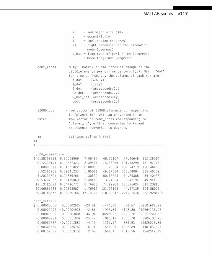
e117MATLAB scripts
a = semimajor axis (AU)
e = eccentricity
i = inclination (degrees)
RA = right ascension of the ascending
node (degrees)
w_hat = longitude of perihelion (degrees)
L = mean longitude (degrees)
cent_rates - 9 by 6 matrix of the rates of change of the
J2000_elements per Julian century (Cy). Using "dot"
for time derivative, the columns of each row are:
a_dot (AU/Cy)
e_dot (1/Cy)
i_dot (arcseconds/Cy)
RA_dot (arcseconds/Cy)
w_hat_dot (arcseconds/Cy)
Ldot (arcseconds/Cy)
J2000_coe - row vector of J2000_elements corresponding
to "planet_id", with au converted to km
rates - row vector of cent_rates corresponding to
"planet_id", with au converted to km and
arcseconds converted to degrees
au - astronomical unit (km)
%}
% ––––––––––––––––––––––––––––––––––––––––––––––––––––––––––––––––––––
J2000_elements = ...
[ 0.38709893 0.20563069 7.00487 48.33167 77.45645 252.25084
0.72333199 0.00677323 3.39471 76.68069 131.53298 181.97973
1.00000011 0.01671022 0.00005 -11.26064 102.94719 100.46435
1.52366231 0.09341233 1.85061 49.57854 336.04084 355.45332
5.20336301 0.04839266 1.30530 100.55615 14.75385 34.40438
9.53707032 0.05415060 2.48446 113.71504 92.43194 49.94432
19.19126393 0.04716771 0.76986 74.22988 170.96424 313.23218
30.06896348 0.00858587 1.76917 131.72169 44.97135 304.88003
39.48168677 0.24880766 17.14175 110.30347 224.06676 238.92881];
cent_rates = ...
[ 0.00000066 0.00002527 -23.51 -446.30 573.57 538101628.29
0.00000092 -0.00004938 -2.86 -996.89 -108.80 210664136.06
-0.00000005 -0.00003804 -46.94 -18228.25 1198.28 129597740.63
-0.00007221 0.00011902 -25.47 -1020.19 1560.78 68905103.78
0.00060737 -0.00012880 -4.15 1217.17 839.93 10925078.35
-0.00301530 -0.00036762 6.11 -1591.05 -1948.89 4401052.95
0.00152025 -0.00019150 -2.09 -1681.4 1312.56 1542547.79
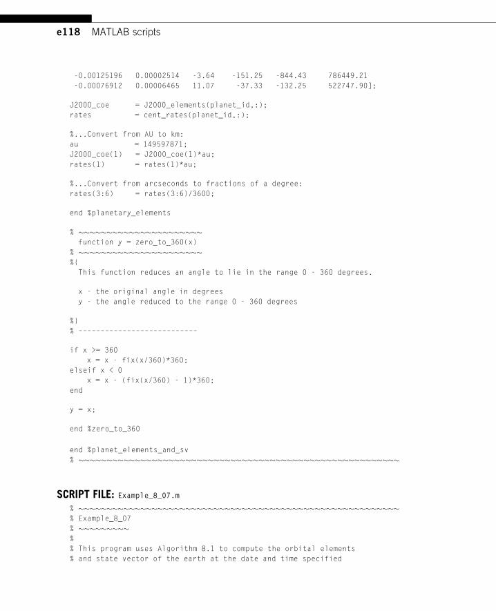
e118 MATLAB scripts
-0.00125196 0.00002514 -3.64 -151.25 -844.43 786449.21
-0.00076912 0.00006465 11.07 -37.33 -132.25 522747.90];
J2000_coe = J2000_elements(planet_id,:);
rates = cent_rates(planet_id,:);
%...Convert from AU to km:
au = 149597871;
J2000_coe(1) = J2000_coe(1)*au;
rates(1) = rates(1)*au;
%...Convert from arcseconds to fractions of a degree:
rates(3:6) = rates(3:6)/3600;
end %planetary_elements
% ����������������������function y = zero_to_360(x)
% ����������������������%{
This function reduces an angle to lie in the range 0 - 360 degrees.
x - the original angle in degrees
y - the angle reduced to the range 0 - 360 degrees
%}
% –––––––––––––––––––––––––––
if x >= 360
x = x - fix(x/360)*360;
elseif x < 0
x = x - (fix(x/360) - 1)*360;
end
y = x;
end %zero_to_360
end %planet_elements_and_sv
% ���������������������������������������������������������
SCRIPT FILE: Example_8_07.m
% ���������������������������������������������������������% Example_8_07
% ���������%
% This program uses Algorithm 8.1 to compute the orbital elements
% and state vector of the earth at the date and time specified
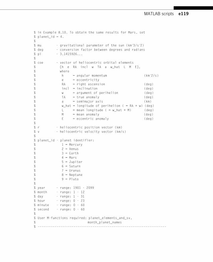
e119MATLAB scripts
% in Example 8.10. To obtain the same results for Mars, set
% planet_id = 4.
%
% mu - gravitational parameter of the sun (km 3̂/s 2̂)
% deg - conversion factor between degrees and radians
% pi - 3.1415926...
%
% coe - vector of heliocentric orbital elements
% [h e RA incl w TA a w_hat L M E],
% where
% h = angular momentum (km 2̂/s)
% e = eccentricity
% RA = right ascension (deg)
% incl = inclination (deg)
% w = argument of perihelion (deg)
% TA = true anomaly (deg)
% a = semimajor axis (km)
% w_hat = longitude of perihelion ( = RA + w) (deg)
% L = mean longitude ( = w_hat + M) (deg)
% M = mean anomaly (deg)
% E = eccentric anomaly (deg)
%
% r - heliocentric position vector (km)
% v - heliocentric velocity vector (km/s)
%
% planet_id - planet identifier:
% 1 = Mercury
% 2 = Venus
% 3 = Earth
% 4 = Mars
% 5 = Jupiter
% 6 = Saturn
% 7 = Uranus
% 8 = Neptune
% 9 = Pluto
%
% year - range: 1901 - 2099
% month - range: 1 - 12
% day - range: 1 - 31
% hour - range: 0 - 23
% minute - range: 0 - 60
% second - range: 0 - 60
%
% User M-functions required: planet_elements_and_sv,
% month_planet_names
% ––––––––––––––––––––––––––––––––––––––––––––––––––––––––––––––––––––
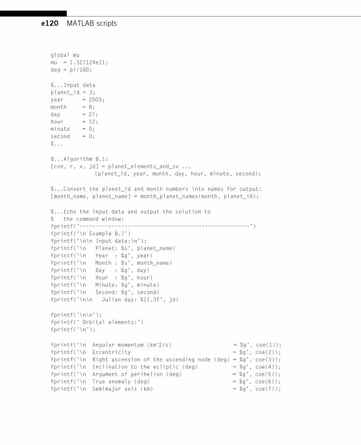
e120 MATLAB scripts
global mu
mu = 1.327124e11;
deg = pi/180;
%...Input data
planet_id = 3;
year = 2003;
month = 8;
day = 27;
hour = 12;
minute = 0;
second = 0;
%...
%...Algorithm 8.1:
[coe, r, v, jd] = planet_elements_and_sv ...
(planet_id, year, month, day, hour, minute, second);
%...Convert the planet_id and month numbers into names for output:
[month_name, planet_name] = month_planet_names(month, planet_id);
%...Echo the input data and output the solution to
% the command window:
fprintf(’–––––––––––––––––––––––––––––––––––––––––––––––––––––’)
fprintf(’\n Example 8.7’)
fprintf(’\n\n Input data:\n’);
fprintf(’\n Planet: %s’, planet_name)
fprintf(’\n Year : %g’, year)
fprintf(’\n Month : %s’, month_name)
fprintf(’\n Day : %g’, day)
fprintf(’\n Hour : %g’, hour)
fprintf(’\n Minute: %g’, minute)
fprintf(’\n Second: %g’, second)
fprintf(’\n\n Julian day: %11.3f’, jd)
fprintf(’\n\n’);
fprintf(’ Orbital elements:’)
fprintf(’\n’);
fprintf(’\n Angular momentum (km 2̂/s) = %g’, coe(1));
fprintf(’\n Eccentricity = %g’, coe(2));
fprintf(’\n Right ascension of the ascending node (deg) = %g’, coe(3));
fprintf(’\n Inclination to the ecliptic (deg) = %g’, coe(4));
fprintf(’\n Argument of perihelion (deg) = %g’, coe(5));
fprintf(’\n True anomaly (deg) = %g’, coe(6));
fprintf(’\n Semimajor axis (km) = %g’, coe(7));
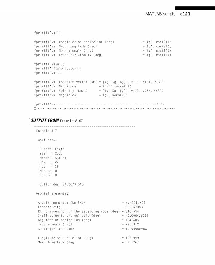
e121MATLAB scripts
fprintf(’\n’);
fprintf(’\n Longitude of perihelion (deg) = %g’, coe(8));
fprintf(’\n Mean longitude (deg) = %g’, coe(9));
fprintf(’\n Mean anomaly (deg) = %g’, coe(10));
fprintf(’\n Eccentric anomaly (deg) = %g’, coe(11));
fprintf(’\n\n’);
fprintf(’ State vector:’)
fprintf(’\n’);
fprintf(’\n Position vector (km) = [%g %g %g]’, r(1), r(2), r(3))
fprintf(’\n Magnitude = %g\n’, norm(r))
fprintf(’\n Velocity (km/s) = [%g %g %g]’, v(1), v(2), v(3))
fprintf(’\n Magnitude = %g’, norm(v))
fprintf(’\n–––––––––––––––––––––––––––––––––––––––––––––––––––––\n’)
% ��������������������������������������������������������
[OUTPUT FROM Example_8_07
–––––––––––––––––––––––––––––––––––––––––––––––––––––
Example 8.7
Input data:
Planet: Earth
Year : 2003
Month : August
Day : 27
Hour : 12
Minute: 0
Second: 0
Julian day: 2452879.000
Orbital elements:
Angular momentum (km 2̂/s) = 4.4551e+09
Eccentricity = 0.0167088
Right ascension of the ascending node (deg) = 348.554
Inclination to the ecliptic (deg) = -0.000426218
Argument of perihelion (deg) = 114.405
True anomaly (deg) = 230.812
Semimajor axis (km) = 1.49598e+08
Longitude of perihelion (deg) = 102.959
Mean longitude (deg) = 335.267
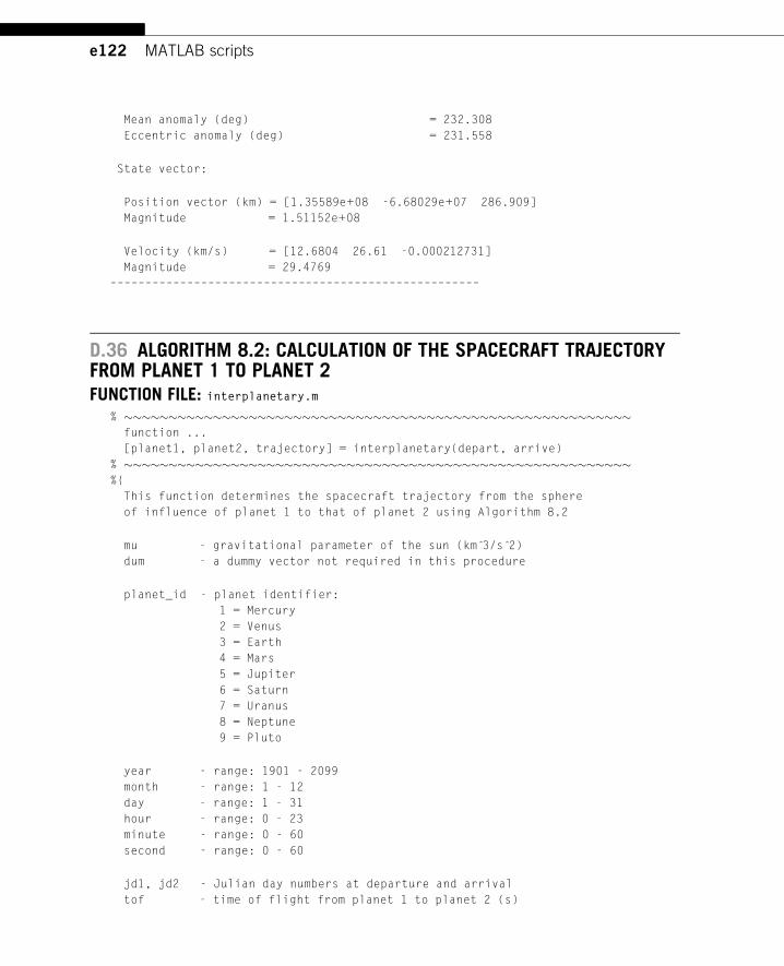
e122 MATLAB scripts
Mean anomaly (deg) = 232.308
Eccentric anomaly (deg) = 231.558
State vector:
Position vector (km) = [1.35589e+08 -6.68029e+07 286.909]
Magnitude = 1.51152e+08
Velocity (km/s) = [12.6804 26.61 -0.000212731]
Magnitude = 29.4769
–––––––––––––––––––––––––––––––––––––––––––––––––––––
D.36 ALGORITHM 8.2: CALCULATION OF THE SPACECRAFT TRAJECTORYFROM PLANET 1 TO PLANET 2FUNCTION FILE: interplanetary.m
% ���������������������������������������������������������function ...
[planet1, planet2, trajectory] = interplanetary(depart, arrive)
% ���������������������������������������������������������%{
This function determines the spacecraft trajectory from the sphere
of influence of planet 1 to that of planet 2 using Algorithm 8.2
mu - gravitational parameter of the sun (km 3̂/s 2̂)
dum - a dummy vector not required in this procedure
planet_id - planet identifier:
1 = Mercury
2 = Venus
3 = Earth
4 = Mars
5 = Jupiter
6 = Saturn
7 = Uranus
8 = Neptune
9 = Pluto
year - range: 1901 - 2099
month - range: 1 - 12
day - range: 1 - 31
hour - range: 0 - 23
minute - range: 0 - 60
second - range: 0 - 60
jd1, jd2 - Julian day numbers at departure and arrival
tof - time of flight from planet 1 to planet 2 (s)
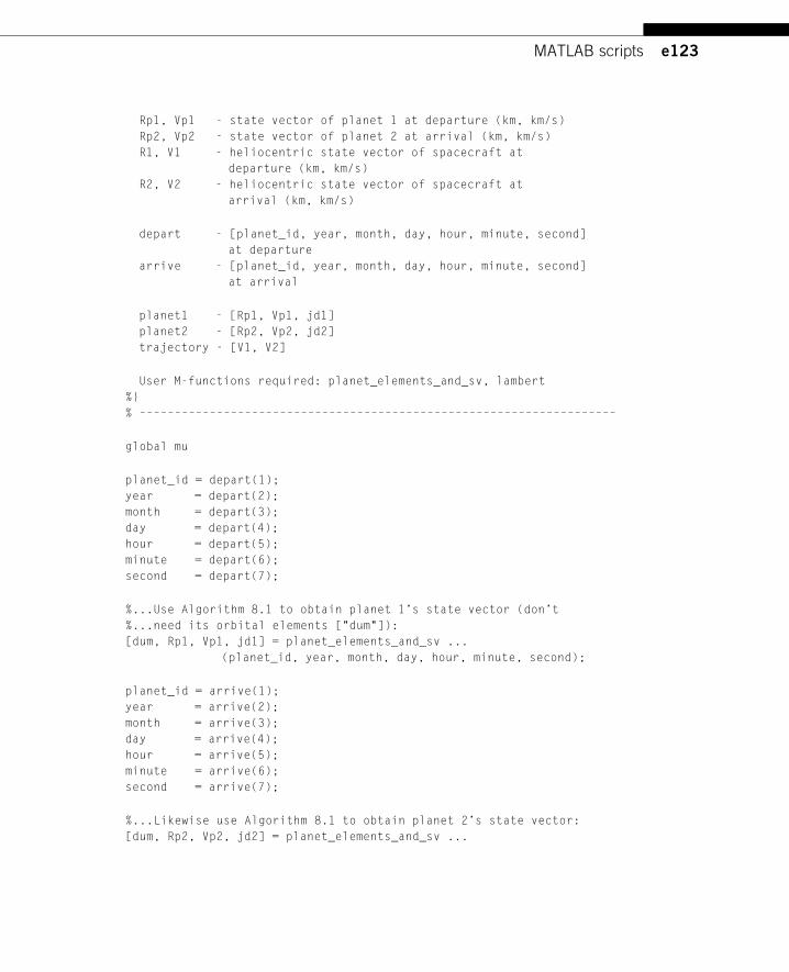
e123MATLAB scripts
Rp1, Vp1 - state vector of planet 1 at departure (km, km/s)
Rp2, Vp2 - state vector of planet 2 at arrival (km, km/s)
R1, V1 - heliocentric state vector of spacecraft at
departure (km, km/s)
R2, V2 - heliocentric state vector of spacecraft at
arrival (km, km/s)
depart - [planet_id, year, month, day, hour, minute, second]
at departure
arrive - [planet_id, year, month, day, hour, minute, second]
at arrival
planet1 - [Rp1, Vp1, jd1]
planet2 - [Rp2, Vp2, jd2]
trajectory - [V1, V2]
User M-functions required: planet_elements_and_sv, lambert
%}
% ––––––––––––––––––––––––––––––––––––––––––––––––––––––––––––––––––––
global mu
planet_id = depart(1);
year = depart(2);
month = depart(3);
day = depart(4);
hour = depart(5);
minute = depart(6);
second = depart(7);
%...Use Algorithm 8.1 to obtain planet 1’s state vector (don’t
%...need its orbital elements ["dum"]):
[dum, Rp1, Vp1, jd1] = planet_elements_and_sv ...
(planet_id, year, month, day, hour, minute, second);
planet_id = arrive(1);
year = arrive(2);
month = arrive(3);
day = arrive(4);
hour = arrive(5);
minute = arrive(6);
second = arrive(7);
%...Likewise use Algorithm 8.1 to obtain planet 2’s state vector:
[dum, Rp2, Vp2, jd2] = planet_elements_and_sv ...
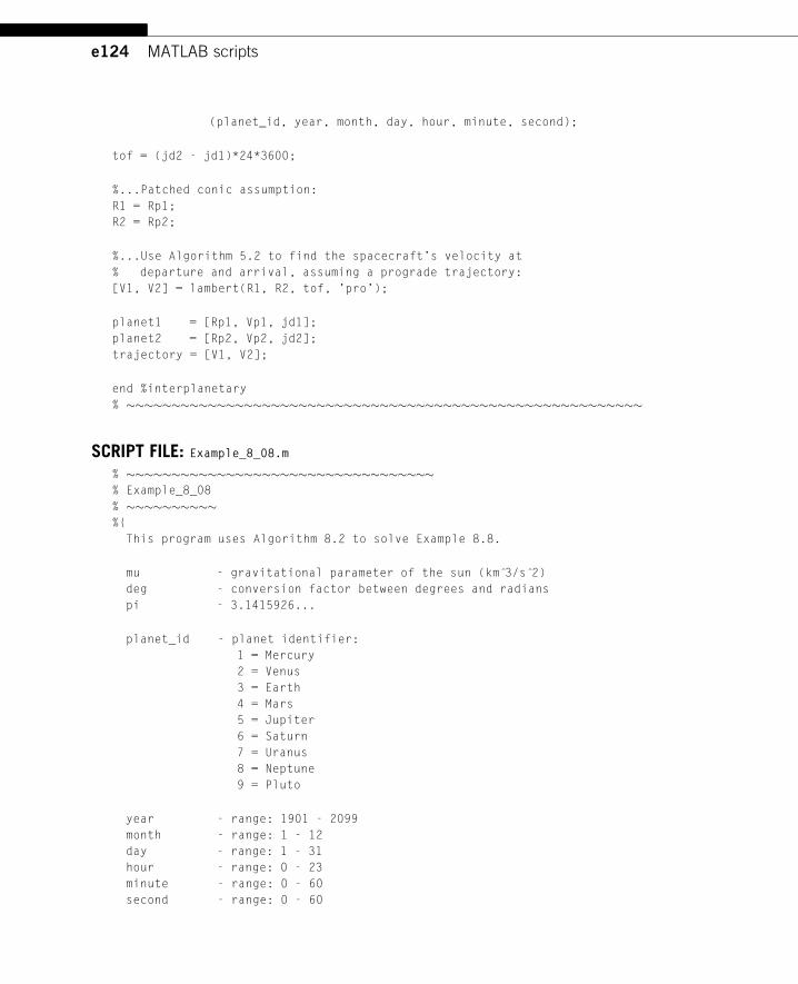
e124 MATLAB scripts
(planet_id, year, month, day, hour, minute, second);
tof = (jd2 - jd1)*24*3600;
%...Patched conic assumption:
R1 = Rp1;
R2 = Rp2;
%...Use Algorithm 5.2 to find the spacecraft’s velocity at
% departure and arrival, assuming a prograde trajectory:
[V1, V2] = lambert(R1, R2, tof, ’pro’);
planet1 = [Rp1, Vp1, jd1];
planet2 = [Rp2, Vp2, jd2];
trajectory = [V1, V2];
end %interplanetary
% ���������������������������������������������������������
SCRIPT FILE: Example_8_08.m
% ����������������������������������% Example_8_08
% ����������%{
This program uses Algorithm 8.2 to solve Example 8.8.
mu - gravitational parameter of the sun (km 3̂/s 2̂)
deg - conversion factor between degrees and radians
pi - 3.1415926...
planet_id - planet identifier:
1 = Mercury
2 = Venus
3 = Earth
4 = Mars
5 = Jupiter
6 = Saturn
7 = Uranus
8 = Neptune
9 = Pluto
year - range: 1901 - 2099
month - range: 1 - 12
day - range: 1 - 31
hour - range: 0 - 23
minute - range: 0 - 60
second - range: 0 - 60
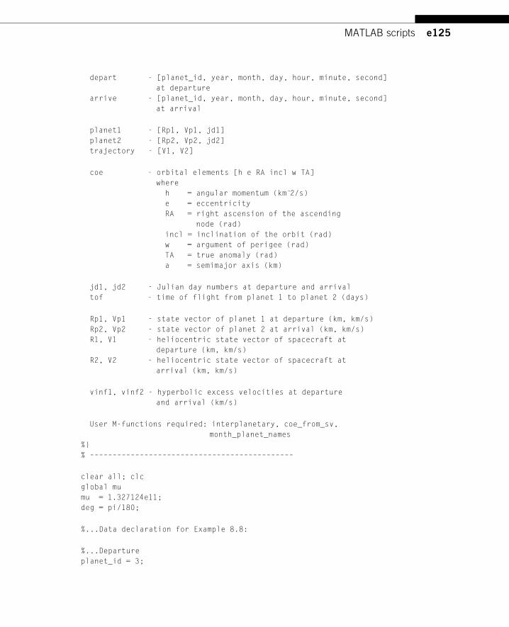
e125MATLAB scripts
depart - [planet_id, year, month, day, hour, minute, second]
at departure
arrive - [planet_id, year, month, day, hour, minute, second]
at arrival
planet1 - [Rp1, Vp1, jd1]
planet2 - [Rp2, Vp2, jd2]
trajectory - [V1, V2]
coe - orbital elements [h e RA incl w TA]
where
h = angular momentum (km 2̂/s)
e = eccentricity
RA = right ascension of the ascending
node (rad)
incl = inclination of the orbit (rad)
w = argument of perigee (rad)
TA = true anomaly (rad)
a = semimajor axis (km)
jd1, jd2 - Julian day numbers at departure and arrival
tof - time of flight from planet 1 to planet 2 (days)
Rp1, Vp1 - state vector of planet 1 at departure (km, km/s)
Rp2, Vp2 - state vector of planet 2 at arrival (km, km/s)
R1, V1 - heliocentric state vector of spacecraft at
departure (km, km/s)
R2, V2 - heliocentric state vector of spacecraft at
arrival (km, km/s)
vinf1, vinf2 - hyperbolic excess velocities at departure
and arrival (km/s)
User M-functions required: interplanetary, coe_from_sv,
month_planet_names
%}
% –––––––––––––––––––––––––––––––––––––––––––––
clear all; clc
global mu
mu = 1.327124e11;
deg = pi/180;
%...Data declaration for Example 8.8:
%...Departure
planet_id = 3;
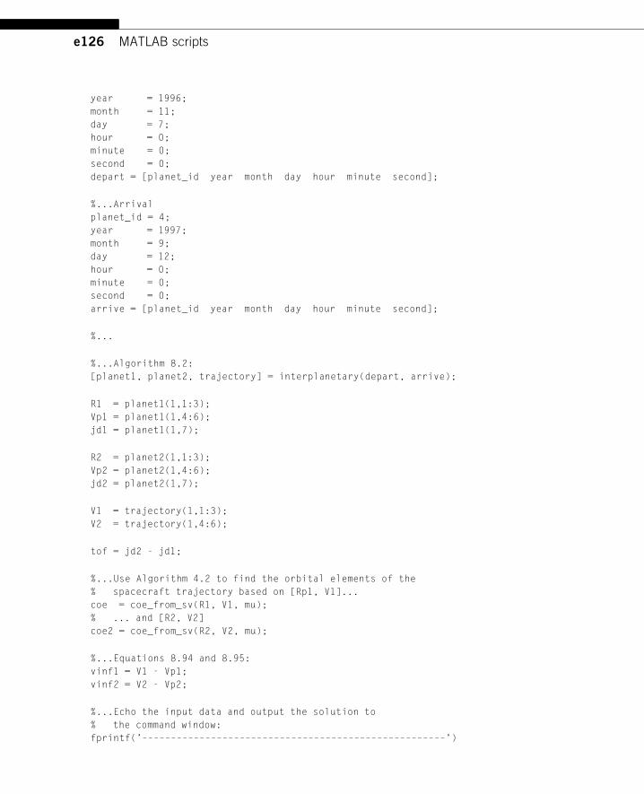
e126 MATLAB scripts
year = 1996;
month = 11;
day = 7;
hour = 0;
minute = 0;
second = 0;
depart = [planet_id year month day hour minute second];
%...Arrival
planet_id = 4;
year = 1997;
month = 9;
day = 12;
hour = 0;
minute = 0;
second = 0;
arrive = [planet_id year month day hour minute second];
%...
%...Algorithm 8.2:
[planet1, planet2, trajectory] = interplanetary(depart, arrive);
R1 = planet1(1,1:3);
Vp1 = planet1(1,4:6);
jd1 = planet1(1,7);
R2 = planet2(1,1:3);
Vp2 = planet2(1,4:6);
jd2 = planet2(1,7);
V1 = trajectory(1,1:3);
V2 = trajectory(1,4:6);
tof = jd2 - jd1;
%...Use Algorithm 4.2 to find the orbital elements of the
% spacecraft trajectory based on [Rp1, V1]...
coe = coe_from_sv(R1, V1, mu);
% ... and [R2, V2]
coe2 = coe_from_sv(R2, V2, mu);
%...Equations 8.94 and 8.95:
vinf1 = V1 - Vp1;
vinf2 = V2 - Vp2;
%...Echo the input data and output the solution to
% the command window:
fprintf(’–––––––––––––––––––––––––––––––––––––––––––––––––––––’)
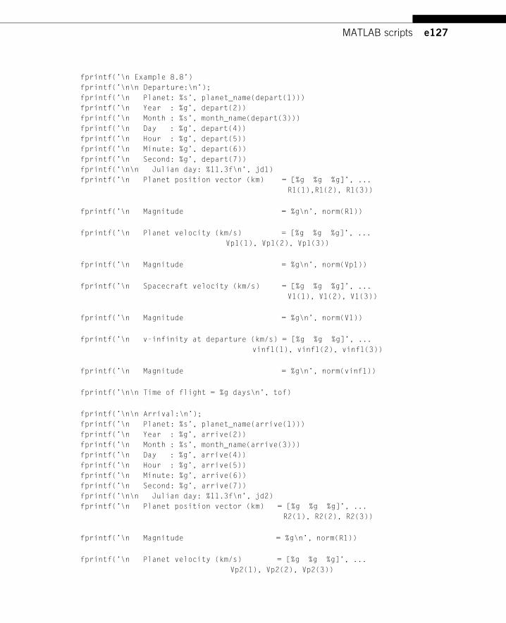
e127MATLAB scripts
fprintf(’\n Example 8.8’)
fprintf(’\n\n Departure:\n’);
fprintf(’\n Planet: %s’, planet_name(depart(1)))
fprintf(’\n Year : %g’, depart(2))
fprintf(’\n Month : %s’, month_name(depart(3)))
fprintf(’\n Day : %g’, depart(4))
fprintf(’\n Hour : %g’, depart(5))
fprintf(’\n Minute: %g’, depart(6))
fprintf(’\n Second: %g’, depart(7))
fprintf(’\n\n Julian day: %11.3f\n’, jd1)
fprintf(’\n Planet position vector (km) = [%g %g %g]’, ...
R1(1),R1(2), R1(3))
fprintf(’\n Magnitude = %g\n’, norm(R1))
fprintf(’\n Planet velocity (km/s) = [%g %g %g]’, ...
Vp1(1), Vp1(2), Vp1(3))
fprintf(’\n Magnitude = %g\n’, norm(Vp1))
fprintf(’\n Spacecraft velocity (km/s) = [%g %g %g]’, ...
V1(1), V1(2), V1(3))
fprintf(’\n Magnitude = %g\n’, norm(V1))
fprintf(’\n v-infinity at departure (km/s) = [%g %g %g]’, ...
vinf1(1), vinf1(2), vinf1(3))
fprintf(’\n Magnitude = %g\n’, norm(vinf1))
fprintf(’\n\n Time of flight = %g days\n’, tof)
fprintf(’\n\n Arrival:\n’);
fprintf(’\n Planet: %s’, planet_name(arrive(1)))
fprintf(’\n Year : %g’, arrive(2))
fprintf(’\n Month : %s’, month_name(arrive(3)))
fprintf(’\n Day : %g’, arrive(4))
fprintf(’\n Hour : %g’, arrive(5))
fprintf(’\n Minute: %g’, arrive(6))
fprintf(’\n Second: %g’, arrive(7))
fprintf(’\n\n Julian day: %11.3f\n’, jd2)
fprintf(’\n Planet position vector (km) = [%g %g %g]’, ...
R2(1), R2(2), R2(3))
fprintf(’\n Magnitude = %g\n’, norm(R1))
fprintf(’\n Planet velocity (km/s) = [%g %g %g]’, ...
Vp2(1), Vp2(2), Vp2(3))
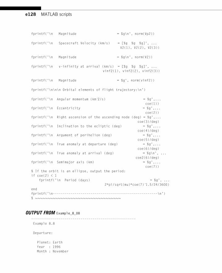
e128 MATLAB scripts
fprintf(’\n Magnitude = %g\n’, norm(Vp2))
fprintf(’\n Spacecraft Velocity (km/s) = [%g %g %g]’, ...
V2(1), V2(2), V2(3))
fprintf(’\n Magnitude = %g\n’, norm(V2))
fprintf(’\n v-infinity at arrival (km/s) = [%g %g %g]’, ...
vinf2(1), vinf2(2), vinf2(3))
fprintf(’\n Magnitude = %g’, norm(vinf2))
fprintf(’\n\n\n Orbital elements of flight trajectory:\n’)
fprintf(’\n Angular momentum (km 2̂/s) = %g’,...
coe(1))
fprintf(’\n Eccentricity = %g’,...
coe(2))
fprintf(’\n Right ascension of the ascending node (deg) = %g’,...
coe(3)/deg)
fprintf(’\n Inclination to the ecliptic (deg) = %g’,...
coe(4)/deg)
fprintf(’\n Argument of perihelion (deg) = %g’,...
coe(5)/deg)
fprintf(’\n True anomaly at departure (deg) = %g’,...
coe(6)/deg)
fprintf(’\n True anomaly at arrival (deg) = %g\n’, ...
coe2(6)/deg)
fprintf(’\n Semimajor axis (km) = %g’,...
coe(7))
% If the orbit is an ellipse, output the period:
if coe(2) < 1
fprintf(’\n Period (days) = %g’, ...
2*pi/sqrt(mu)*coe(7) 1̂.5/24/3600)
end
fprintf(’\n–––––––––––––––––––––––––––––––––––––––––––––––––––––\n’)
% ����������������������������������
OUTPUT FROM Example_8_08
–––––––––––––––––––––––––––––––––––––––––––––––––––––
Example 8.8
Departure:
Planet: Earth
Year : 1996
Month : November
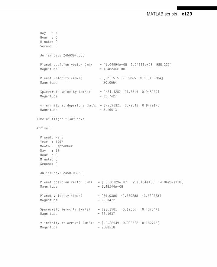
e129MATLAB scripts
Day : 7
Hour : 0
Minute: 0
Second: 0
Julian day: 2450394.500
Planet position vector (km) = [1.04994e+08 1.04655e+08 988.331]
Magnitude = 1.48244e+08
Planet velocity (km/s) = [-21.515 20.9865 0.000132284]
Magnitude = 30.0554
Spacecraft velocity (km/s) = [-24.4282 21.7819 0.948049]
Magnitude = 32.7427
v-infinity at departure (km/s) = [-2.91321 0.79542 0.947917]
Magnitude = 3.16513
Time of flight = 309 days
Arrival:
Planet: Mars
Year : 1997
Month : September
Day : 12
Hour : 0
Minute: 0
Second: 0
Julian day: 2450703.500
Planet position vector (km) = [-2.08329e+07 -2.18404e+08 -4.06287e+06]
Magnitude = 1.48244e+08
Planet velocity (km/s) = [25.0386 -0.220288 -0.620623]
Magnitude = 25.0472
Spacecraft Velocity (km/s) = [22.1581 -0.19666 -0.457847]
Magnitude = 22.1637
v-infinity at arrival (km/s) = [-2.88049 0.023628 0.162776]
Magnitude = 2.88518
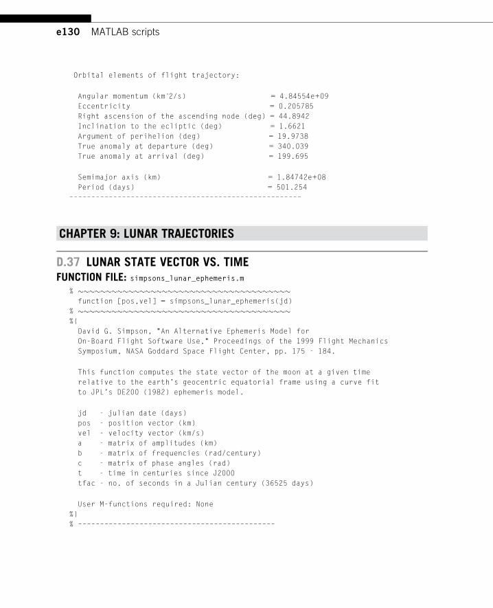
e130 MATLAB scripts
Orbital elements of flight trajectory:
Angular momentum (km 2̂/s) = 4.84554e+09
Eccentricity = 0.205785
Right ascension of the ascending node (deg) = 44.8942
Inclination to the ecliptic (deg) = 1.6621
Argument of perihelion (deg) = 19.9738
True anomaly at departure (deg) = 340.039
True anomaly at arrival (deg) = 199.695
Semimajor axis (km) = 1.84742e+08
Period (days) = 501.254
–––––––––––––––––––––––––––––––––––––––––––––––––––––
CHAPTER 9: LUNAR TRAJECTORIES
D.37 LUNAR STATE VECTOR VS. TIMEFUNCTION FILE: simpsons_lunar_ephemeris.m
% ��������������������������������������function [pos,vel] = simpsons_lunar_ephemeris(jd)
% ��������������������������������������%{
David G. Simpson, "An Alternative Ephemeris Model for
On-Board Flight Software Use," Proceedings of the 1999 Flight Mechanics
Symposium, NASA Goddard Space Flight Center, pp. 175 - 184.
This function computes the state vector of the moon at a given time
relative to the earth’s geocentric equatorial frame using a curve fit
to JPL’s DE200 (1982) ephemeris model.
jd - julian date (days)
pos - position vector (km)
vel - velocity vector (km/s)
a - matrix of amplitudes (km)
b - matrix of frequencies (rad/century)
c - matrix of phase angles (rad)
t - time in centuries since J2000
tfac - no. of seconds in a Julian century (36525 days)
User M-functions required: None
%}
% –––––––––––––––––––––––––––––––––––––––––––––
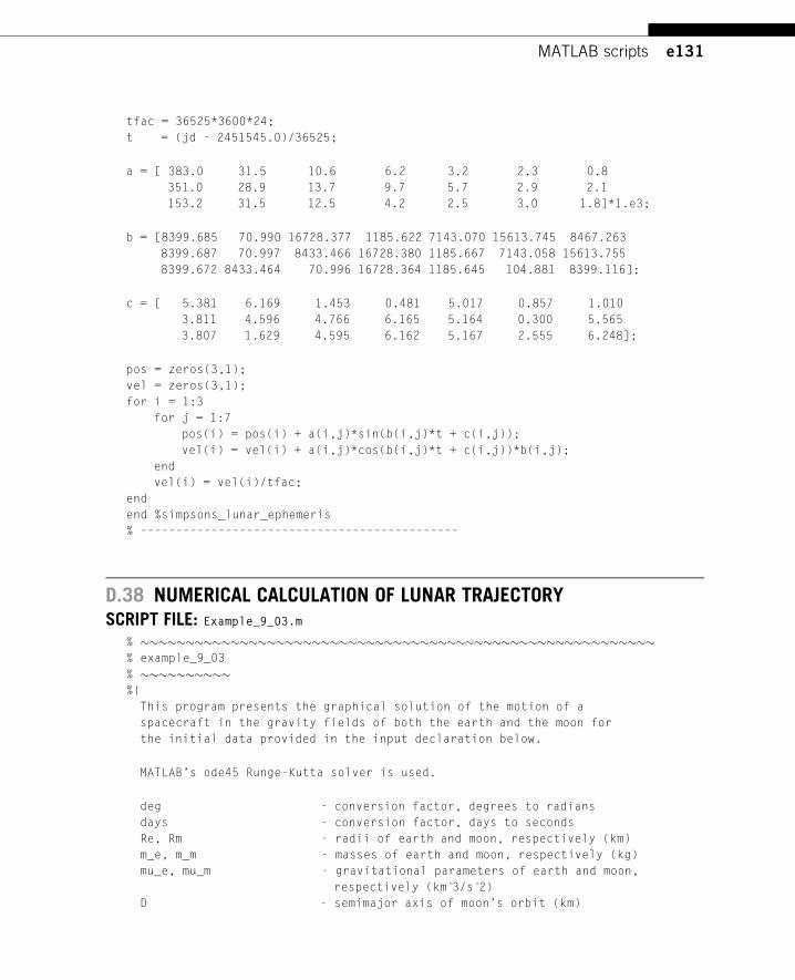
e131MATLAB scripts
tfac = 36525*3600*24;
t = (jd - 2451545.0)/36525;
a = [ 383.0 31.5 10.6 6.2 3.2 2.3 0.8
351.0 28.9 13.7 9.7 5.7 2.9 2.1
153.2 31.5 12.5 4.2 2.5 3.0 1.8]*1.e3;
b = [8399.685 70.990 16728.377 1185.622 7143.070 15613.745 8467.263
8399.687 70.997 8433.466 16728.380 1185.667 7143.058 15613.755
8399.672 8433.464 70.996 16728.364 1185.645 104.881 8399.116];
c = [ 5.381 6.169 1.453 0.481 5.017 0.857 1.010
3.811 4.596 4.766 6.165 5.164 0.300 5.565
3.807 1.629 4.595 6.162 5.167 2.555 6.248];
pos = zeros(3,1);
vel = zeros(3,1);
for i = 1:3
for j = 1:7
pos(i) = pos(i) + a(i,j)*sin(b(i,j)*t + c(i,j));
vel(i) = vel(i) + a(i,j)*cos(b(i,j)*t + c(i,j))*b(i,j);
end
vel(i) = vel(i)/tfac;
end
end %simpsons_lunar_ephemeris
% –––––––––––––––––––––––––––––––––––––––––––––
D.38 NUMERICAL CALCULATION OF LUNAR TRAJECTORYSCRIPT FILE: Example_9_03.m
% ���������������������������������������������������������% example_9_03
% ����������%{
This program presents the graphical solution of the motion of a
spacecraft in the gravity fields of both the earth and the moon for
the initial data provided in the input declaration below.
MATLAB’s ode45 Runge-Kutta solver is used.
deg - conversion factor, degrees to radians
days - conversion factor, days to seconds
Re, Rm - radii of earth and moon, respectively (km)
m_e, m_m - masses of earth and moon, respectively (kg)
mu_e, mu_m - gravitational parameters of earth and moon,
respectively (km 3̂/s 2̂)
D - semimajor axis of moon’s orbit (km)
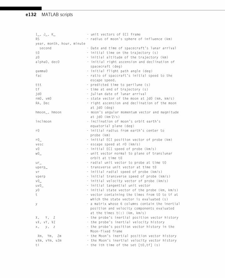
e132 MATLAB scripts
I_, J_, K_ - unit vectors of ECI frame
RS - radius of moon’s sphere of influence (km)
year, month, hour, minute
second - Date and time of spacecraft’s lunar arrival
t0 - initial time on the trajectory (s)
z0 - initial altitude of the trajectory (km)
alpha0, dec0 - initial right ascension and declination of
spacecraft (deg)
gamma0 - initial flight path angle (deg)
fac - ratio of spaccraft’s initial speed to the
escape speed.
ttt - predicted time to perilune (s)
tf - time at end of trajectory (s)
jd0 - julian date of lunar arrival
rm0, vm0 - state vector of the moon at jd0 (km, km/s)
RA, Dec - right ascension and declination of the moon
at jd0 (deg)
hmoon_, hmoon - moon’s angular momentum vector and magnitude
at jd0 (km 2̂/s)
inclmoon - inclination of moon’s orbit earth’s
equatorial plane (deg)
r0 - initial radius from earth’s center to
probe (km)
r0_ - initial ECI position vector of probe (km)
vesc - escape speed at r0 (km/s)
v0 - initial ECI speed of probe (km/s)
w0_ - unit vector normal to plane of translunar
orbit at time t0
ur_ - radial unit vector to probe at time t0
uperp_ - transverse unit vector at time t0
vr - initial radial speed of probe (km/s)
vperp - initial transverse speed of probe (km/s)
v0_ - initial velocity vector of probe (km/s)
uv0_ - initial tangential unit vector
y0 - initial state vector of the probe (km, km/s)
t - vector containing the times from t0 to tf at
which the state vector is evaluated (s)
y - a matrix whose 6 columns contain the inertial
position and velocity components evaluated
at the times t(:) (km, km/s)
X, Y, Z - the probe’s inertial position vector history
vX, vY, VZ - the probe’s inertial velocity history
x, y, z - the probe’s position vector history in the
Moon-fixed frame
Xm, Ym, Zm - the Moon’s inertial position vector history
vXm, vYm, vZm - the Moon’s inertial velocity vector history
ti - the ith time of the set [t0,tf] (s)
e133MATLAB scripts
r_ - probe’s inertial position vector at time ti
(km)
r - magnitude of r_ (km)
jd - julian date of corresponding to ti (days)
rm_, vm_ - the moon’s state vector at time ti (km,km/s)
x_, y_, z_ - vectors along the axes of the rotating
moon-fixed at time ti (km)
i_, j_, k_ - unit vectors of the moon-fixed rotating frame
at time ti
Q - DCM of transformation from ECI to moon-fixed
frame at time ti
rx_ - probe’s inertial position vector in moon-
fixed coordinates at time ti (km)
rmx_ - Moon’s inertial position vector in moon-
fixed coordinates at time ti (km)
dist_ - position vector of probe relative to the moon
at time ti (km)
dist - magnitude of dist_ (km)
dist_min - perilune of trajectory (km)
rmTLI_ - Moon’s position vector at TLI
RATLI, DecTLI - Moon’s right ascension and declination at
TKI (deg)
v_atdmin_ - Probe’s velocity vector at perilune (km/s)
rm_perilume, vm_perilune - Moon’s state vector when the probe is at
perilune (km, km/s)
rel_speed - Speed of probe relative to the Moon at
perilune (km/s)
RA_at_perilune - Moon’s RA at perilune arrival (deg)
Dec_at_perilune - Moon’s Dec at perilune arrival (deg)
target_error - Distance between Moon’s actual position at
perilune arrival and its position after the
predicted flight time, ttt (km).
rms_ - position vector of moon relative to
spacecraft (km)
rms - magnitude of rms_ (km)
aearth_ - acceleration of spacecraft due to
earth (km/s 2̂)
amoon_ - acceleration of spacecraft due to
moon (km/s 2̂)
atot_ - aearth_ + amoon_ (km/s 2̂)
binormal_ - unit vector normal to the osculating plane
incl - angle between inertial Z axis and the
binormal (deg)
rend_ - Position vector of end point of trajectory
(km)
alt_end - Altitude of end point of trajectory (km)
ra_end, dec_end - Right ascension and declination of end point
of trajectory (km)
e134 MATLAB scripts
User M-functions required: none
User subfunctions required: rates, plotit_XYZ, plotit_xyz
%}
% ––––––––––––––––––––––––––––––––––––––––––––––––––––––––––––––––––––
clear all; close all; clc
fprintf(’\nlunar_restricted_threebody.m %s\n\n’, datestr(now))
global jd0 days ttt mu_m mu_e Re Rm rm_ rm0_
%...general data
deg = pi/180;
days = 24*3600;
Re = 6378;
Rm = 1737;
m_e = 5974.e21;
m_m = 73.48e21;
mu_e = 398600.4;
mu_m = 4902.8;
D = 384400;
RS = D*(m_m/m_e) (̂2/5);
%...
%...Data declaration for Example 9.03
Title = ’Example 9.3 4e’;
% Date and time of lunar arrival:
year = 2020;
month = 5;
day = 4;
hour = 12;
minute = 0;
second = 0;
t0 = 0;
z0 = 320;
alpha0 = 90;
dec0 = 15;
gamma0 = 40;
fac = .9924; %Fraction of Vesc
ttt = 3*days;
tf = ttt + 2.667*days;
%...End data declaration
%...State vector of moon at target date:
jd0 = juliandate(year, month, day, hour, minute, second);
[rm0_,vm0_] = simpsons_lunar_ephemeris(jd0);
%[rm0_,vm0] = planetEphemeris(jd0, ’Earth’, ’Moon’, ’430’);
[RA, Dec] = ra_and_dec_from_r(rm0_);
e135MATLAB scripts
distance = norm(rm0_);
hmoon_ = cross(rm0_,vm0_);
hmoon = norm(hmoon_);
inclmoon = acosd(hmoon_(3)/hmoon);
%...Initial position vector of probe:
I_ = [1;0;0];
J_ = [0;1;0];
K_ = cross(I_,J_);
r0 = Re + z0;
r0_ = r0*(cosd(alpha0)*cosd(dec0)*I_ + ...
sind(alpha0)*cosd(dec0)*J_ + ...
sind(dec0)*K_);
vesc = sqrt(2*mu_e/r0);
v0 = fac*vesc;
w0_ = cross(r0_,rm0_)/norm(cross(r0_,rm0_));
%...Initial velocity vector of probe:
ur_ = r0_/norm(r0_);
uperp_ = cross(w0_,ur_)/norm(cross(w0_,ur_));
vr = v0*sind(gamma0);
vperp = v0*cosd(gamma0);
v0_ = vr*ur_ + vperp*uperp_;
uv0_ = v0_/v0;
%...Initial state vector of the probe:
y0 = [r0_(1) r0_(2) r0_(3) v0_(1) v0_(2) v0_(3)]’;
%...Pass the initial conditions and time interval to ode45, which
% calculates the position and velocity of the spacecraft at discrete
% times t, returning the solution in the column vector y. ode45 uses
% the subfunction ’rates’ below to evaluate the spacecraft acceleration
% at each integration time step.
options = odeset(’RelTol’, 1.e-10, ’AbsTol’, 1.e-10,’Stats’, ’off’);
[t,y] = ode45(@rates, [t0 tf], y0, options);
%...Spacecraft trajectory
% in ECI frame:
X = y(:,1); Y = y(:,2); Z = y(:,3);
vX = y(:,4); vY = y(:,5); vZ = y(:,6);
% in Moon-fixed frame:
x = []; y = []; z = [];
%...Moon trajectory
% in ECI frame:
Xm = []; Ym = []; Zm = [];
e136 MATLAB scripts
vXm = []; vYm = []; vZm = [];
% in Moon-fixed frame:
xm = []; ym = []; zm = [];
%...Compute the Moon’s trajectory from an ephemeris, find perilune of the
% probe’s trajectory, and project the probe’s trajectory onto the axes
% of the Moon-fixed rotating frame:
dist_min = 1.e30; %Starting value in the search for perilune
for i = 1:length(t)
ti = t(i);
%...Probe’s inertial position vector at time ti:
r_ = [X(i) Y(i) Z(i)]’;
%...Moon’s inertial position and velocity vectors at time ti:
jd = jd0 - (ttt - ti)/days;
[rm_,vm_] = simpsons_lunar_ephemeris(jd);
%...Moon’s inertial state vector at time ti:
Xm = [ Xm;rm_(1)]; Ym = [ Ym;rm_(2)]; Zm = [ Zm;rm_(3)];
vXm = [vXm;vm_(1)]; vYm = [vYm;vm_(2)]; vZm = [vZm;vm_(3)];
%...Moon-fixed rotating xyz frame:
x_ = rm_;
z_ = cross(x_,vm_);
y_ = cross(z_,x_);
i_ = x_/norm(x_);
j_ = y_/norm(y_);
k_ = z_/norm(z_);
%...DCM of transformation from ECI to moon-fixed frame:
Q = [i_’; j_’; k_’];
%...Components of probe’s inertial position vector in moon-fixed frame:
rx_ = Q*r_;
x = [x;rx_(1)]; y = [y;rx_(2)]; z = [z;rx_(3)];
%...Components of moon’s inertial position vector in moon-fixed frame:
rmx_ = Q*rm_;
xm = [xm;rmx_(1)]; ym = [ym;rmx_(2)]; zm = [zm;rmx_(3)];
%...Find perilune of the probe:
dist_ = r_ - rm_;
dist = norm(dist_);
if dist < dist_min
imin = i;
e137MATLAB scripts
dist_min_ = dist_;
dist_min = dist;
end
end
%...Location of the Moon at TLI:
rmTLI_ = [Xm(1); Ym(1); Zm(1)];
[RATLI, DecTLI] = ra_and_dec_from_r(rmTLI_);
%...Spacecraft velocity at perilune:
v_atdmin_ = [vX(imin);vY(imin);vZ(imin)];
%...State vector and celestial position of moon when probe is at perilune:
rm_perilune_ = [Xm(imin) Ym(imin) Zm(imin)]’;
vm_perilune_ = [vXm(imin) vYm(imin) vZm(imin)]’;
[RA_at_perilune, Dec_at_perilune] = ra_and_dec_from_r(rm_perilune_);
target_error = norm(rm_perilune_ - rm0_);
%...Speed of probe relative to Moon at perilune:
rel_speed = norm(v_atdmin_ - vm_perilune_);
%...End point of trajectory:
rend_ = [X(end); Y(end); Z(end)];
alt_end = norm(rend_) - Re;
[ra_end, dec_end] = ra_and_dec_from_r(rend_);
%...Find the history of the trajectory’s binormal:
for i = 1:imin
time(i) = t(i);
r_ = [X(i) Y(i) Z(i)]’;
r = norm(r_);
v_ = [vX(i) vY(i) vZ(i)]’;
rm_ = [Xm(i) Ym(i) Zm(i)]’;
rm = norm(rm_);
rms_ = rm_ - r_;
rms(i) = norm(rms_);
aearth_ = -mu_e*r_/r 3̂;
amoon_ = mu_m*(rms_/rms(i) 3̂ - rm_/rm 3̂);
atot_ = aearth_ + amoon_;
binormal_ = cross(v_,atot_)/norm(cross(v_,atot_));
binormalz = binormal_(3);
incl(i) = acosd(binormalz);
end
%...Output:
fprintf(’\n\n%s\n\n’, Title)
e138 MATLAB scripts
fprintf(’Date and time of arrival at moon: ’)
fprintf(’%s/%s/%s %s:%s:%s’, ...
num2str(month), num2str(day), num2str(year), ...
num2str(hour), num2str(minute), num2str(second))
fprintf(’\nMoon’’s position: ’)
fprintf(’\n Distance = %11g km’ , distance)
fprintf(’\n Right Ascension = %11g deg’ , RA)
fprintf(’\n Declination = %11g deg ’ , Dec)
fprintf(’\nMoon’’s orbital inclination = %11g deg\n’ , inclmoon)
fprintf(’\nThe probe at earth departure (t = %g sec):’, t0)
fprintf(’\n Altitude = %11g km’ , z0)
fprintf(’\n Right ascension = %11g deg’ , alpha0)
fprintf(’\n Declination = %11g deg’ , dec0)
fprintf(’\n Flight path angle = %11g deg’ , gamma0)
fprintf(’\n Speed = %11g km/s’ , v0)
fprintf(’\n Escape speed = %11g km/s’ , vesc)
fprintf(’\n v/vesc = %11g’ , v0/vesc)
fprintf(’\n Inclination of translunar orbit = %11g deg\n’ , ...
acosd(w0_(3)))
fprintf(’\nThe moon when the probe is at TLI:’)
fprintf(’\n Distance = %11g km’ , norm(rmTLI_))
fprintf(’\n Right ascension = %11g deg’, RATLI)
fprintf(’\n Declination = %11g deg’, DecTLI)
fprintf(’\nThe moon when the probe is at perilune: ’)
fprintf(’\n Distance = %11g km’ , ...
norm(rm_perilune_))
fprintf(’\n Speed = %11g km/s’, ...
norm(vm_perilune_))
fprintf(’\n Right ascension = %11g deg’ ,RA_at_perilune)
fprintf(’\n Declination = %11g deg’ ,Dec_at_perilune)
fprintf(’\n Target error = %11g km’ , target_error)
fprintf(’\n\nThe probe at perilune:’)
fprintf(’\n Altitude = %11g km’ , dist_min - Rm)
fprintf(’\n Speed = %11g km/s’,norm(v_atdmin_))
fprintf(’\n Relative speed = %11g km/s’,rel_speed)
fprintf(’\n Inclination of osculating plane = %11g deg’ ,incl(imin))
fprintf(’\n Time from TLI to perilune = %11g hours (%g days)’ ...
abs(t(imin))/3600 ...
abs(t(imin))/3600/24)
fprintf(’\n\nTotal time of flight = %11g days’ , t(end)/days)
fprintf(’\nTime to target point = %11g days’ , ttt/days)
e139MATLAB scripts
fprintf(’\nFinal earth altitude = %11g km’ , alt_end)
fprintf(’\nFinal right ascension = %11g deg’ , ra_end)
fprintf(’\nFinal declination = %11g deg\n’ , dec_end)
%...End output
%...Graphical output"
% Plot the trajectory relative to the inertial frame:
plotit_XYZ(X,Y,Z,Xm,Ym,Zm,imin)
% Plot inclination of the osculating plane vs distance from the Moon
figure
hold on
plot(rms/RS,incl)
line([0 6][90 90],’Linestyle’,’–’,’color’,’red’)
title(’Osculating Plane Inclination vs Distance from Moon’)
xlabel(’r_{ms}/R_s’)
ylabel(’Inclination deg)’)
grid on
grid minor
% Plot the trajectory relative to the rotating Moon-fixed frame:
plotit_xyz(x,y,z,xm,ym,zm,imin)
%...End graphical output
return
% ������������������������������������������������������������function dydt = rates(t,y)
% ��������������������%{
This function evaluates the 3D acceleration of the spacecraft in a
restricted 3-body system at time t from its position and velocity
and the position of the moon at that time.
t - time (s)
ttt - flight time, TLI to target point (s)
jd0 - Julian Date on arrival at target (days)
jd - Julian Date at time t (days)
X, Y, Z - Components of spacecraft’s geocentric position vector (km)
vX, vY, vZ - Components of spacecraft’s geocentric velocity vector (km/s)
aX, aY, aZ - Components of spacecraft’s geocentric acceleration
vector (km/s 2̂)
y - column vector containing the geocentric position and
velocity components of the spacecraft at time t
r_ - geocentric position vector [X Y Z] of the spacecraft
rm_ - geocentric position vector of the moon
rms_ - rm_ - r_, the position of the moon relative to the
spacecraft
e140 MATLAB scripts
aearth_ - spacecraft acceleration vector due to earth’s gravity
amoon_ - spacecraft acceleration vector due to lunar gravity
a_ - total spacececraft acceleration vector
dydt - column vector containing the geocentric velocity and
acceleration components of the spacecraft at time t
%}
% ––––––––––––––––––––––––––––––––––––––––––––––––––––––––––––––––––––
global jd0 days mu_m mu_e ttt
jd = jd0 - (ttt - t)/days;
X = y(1);
Y = y(2);
Z = y(3);
vX = y(4);
vY = y(5);
vZ = y(6);
r_ = [X Y Z]’;
r = norm(r_);
[rm_,�] = simpsons_lunar_ephemeris(jd);
%[rm_,�] = planetEphemeris(jd0, ’Earth’, ’Moon’, ’430’);
rm = norm(rm_);
rms_ = rm_ - r_;
rms = norm(rms_);
aearth_ = -mu_e*r_/r 3̂;
amoon_ = mu_m*(rms_/rms 3̂ - rm_/rm 3̂);
a_ = aearth_ + amoon_;
aX = a_(1);
aY = a_(2);
aZ = a_(3);
dydt = [vX vY vZ aX aY aZ]’;
end %rates
% ������������������������������������������������������������
% ������������������������������function plotit_XYZ(X,Y,Z,Xm,Ym,Zm,imin)
% ––––––––––––––––––––––––––––––––––––––
global Re Rm
figure (’Name’,’Trajectories of Spacecraft (red) and Moon (green)’, ...
’Color’, [1 1 1])
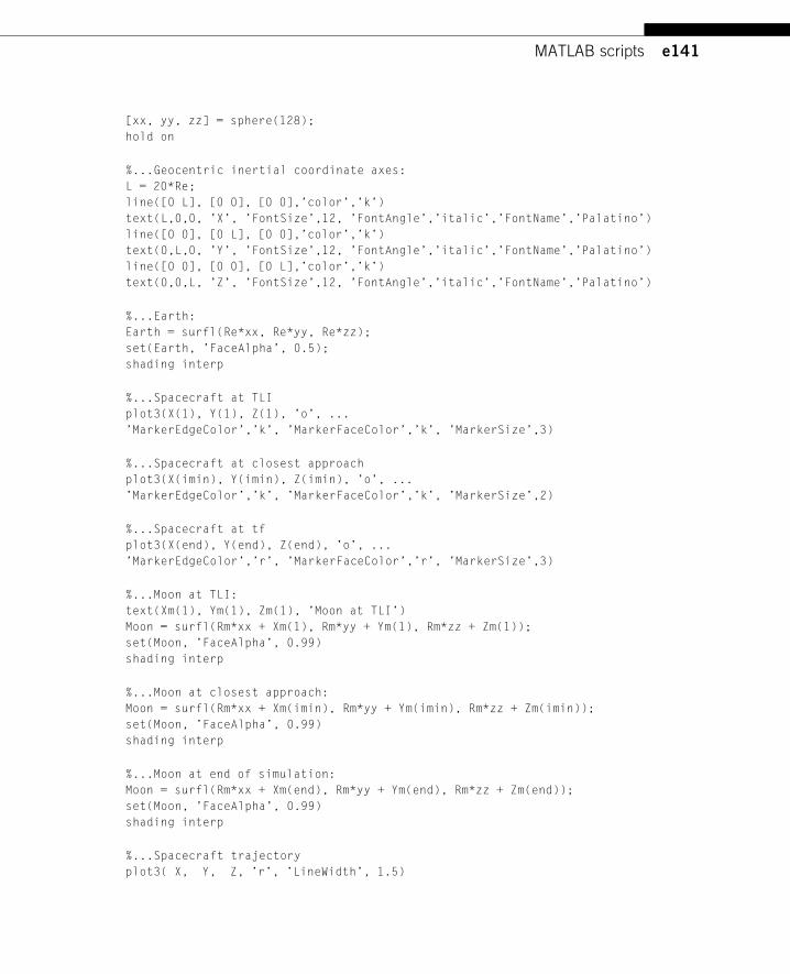
e141MATLAB scripts
[xx, yy, zz] = sphere(128);
hold on
%...Geocentric inertial coordinate axes:
L = 20*Re;
line([0 L], [0 0], [0 0],’color’,’k’)
text(L,0,0, ’X’, ’FontSize’,12, ’FontAngle’,’italic’,’FontName’,’Palatino’)
line([0 0], [0 L], [0 0],’color’,’k’)
text(0,L,0, ’Y’, ’FontSize’,12, ’FontAngle’,’italic’,’FontName’,’Palatino’)
line([0 0], [0 0], [0 L],’color’,’k’)
text(0,0,L, ’Z’, ’FontSize’,12, ’FontAngle’,’italic’,’FontName’,’Palatino’)
%...Earth:
Earth = surfl(Re*xx, Re*yy, Re*zz);
set(Earth, ’FaceAlpha’, 0.5);
shading interp
%...Spacecraft at TLI
plot3(X(1), Y(1), Z(1), ’o’, ...
’MarkerEdgeColor’,’k’, ’MarkerFaceColor’,’k’, ’MarkerSize’,3)
%...Spacecraft at closest approach
plot3(X(imin), Y(imin), Z(imin), ’o’, ...
’MarkerEdgeColor’,’k’, ’MarkerFaceColor’,’k’, ’MarkerSize’,2)
%...Spacecraft at tf
plot3(X(end), Y(end), Z(end), ’o’, ...
’MarkerEdgeColor’,’r’, ’MarkerFaceColor’,’r’, ’MarkerSize’,3)
%...Moon at TLI:
text(Xm(1), Ym(1), Zm(1), ’Moon at TLI’)
Moon = surfl(Rm*xx + Xm(1), Rm*yy + Ym(1), Rm*zz + Zm(1));
set(Moon, ’FaceAlpha’, 0.99)
shading interp
%...Moon at closest approach:
Moon = surfl(Rm*xx + Xm(imin), Rm*yy + Ym(imin), Rm*zz + Zm(imin));
set(Moon, ’FaceAlpha’, 0.99)
shading interp
%...Moon at end of simulation:
Moon = surfl(Rm*xx + Xm(end), Rm*yy + Ym(end), Rm*zz + Zm(end));
set(Moon, ’FaceAlpha’, 0.99)
shading interp
%...Spacecraft trajectory
plot3( X, Y, Z, ’r’, ’LineWidth’, 1.5)

e142 MATLAB scripts
%...Moon trajectory
plot3(Xm, Ym, Zm, ’g’, ’LineWidth’, 0.5)
axis image
axis off
axis vis3d
view([1,1,1])
end %plotit_XYZ
% ����������
% ������������������������������function plotit_xyz(x,y,z,xm,ym,zm,imin)
% ––––––––––––––––––––––––––––––––––––––
global Re Rm Rm0_ Q0
figure (’Name’,’Spacecraft trajectory in Moon-fixed rotating frame’, ...
’Color’, [1 1 1])
[xx, yy, zz] = sphere(128);
hold on
%...Spacecraft trajectory:
plot3( x, y, z, ’r’, ’LineWidth’, 2.0)
%...Moon trajectory:
plot3(xm, ym, zm, ’g’, ’LineWidth’, 0.5)
%...Earth:
Earth = surfl(Re*xx, Re*yy, Re*zz);
set(Earth, ’FaceAlpha’, 0.5);
shading interp
%...Geocentric moon-fixed coordinate axes:
L1 = 63*Re; L2 = 20*Re; L3 = 29*Re;
line([0 L1], [0 0], [0 0],’color’,’k’)
text(L1, 0, 0, ’x’,’FontSize’, 12, ’FontAngle’, ’italic’,’FontName’,’Palatino’)
line([0 0], [0 L2], [0 0],’color’,’k’)
text(0, L2, 0, ’y’,’FontSize’, 12, ’FontAngle’, ’italic’,’FontName’,’Palatino’)
line([0 0], [0 0], [0 L3],’color’,’k’)
text(0, 0, L3, ’z’,’FontSize’, 12, ’FontAngle’, ’italic’,’FontName’,’Palatino’)
%...Spacecraft at TLI
plot3(x(1), y(1), z(1), ’o’, ...
’MarkerEdgeColor’,’k’, ’MarkerFaceColor’,’k’, ’MarkerSize’,3)
%...Spacecraft at closest approach
plot3(x(imin), y(imin), z(imin), ’o’, ...
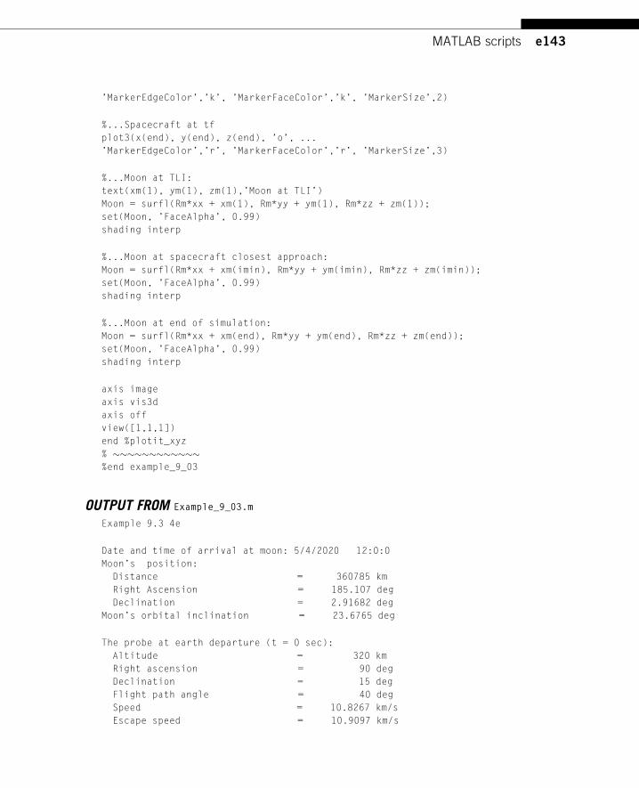
e143MATLAB scripts
’MarkerEdgeColor’,’k’, ’MarkerFaceColor’,’k’, ’MarkerSize’,2)
%...Spacecraft at tf
plot3(x(end), y(end), z(end), ’o’, ...
’MarkerEdgeColor’,’r’, ’MarkerFaceColor’,’r’, ’MarkerSize’,3)
%...Moon at TLI:
text(xm(1), ym(1), zm(1),’Moon at TLI’)
Moon = surfl(Rm*xx + xm(1), Rm*yy + ym(1), Rm*zz + zm(1));
set(Moon, ’FaceAlpha’, 0.99)
shading interp
%...Moon at spacecraft closest approach:
Moon = surfl(Rm*xx + xm(imin), Rm*yy + ym(imin), Rm*zz + zm(imin));
set(Moon, ’FaceAlpha’, 0.99)
shading interp
%...Moon at end of simulation:
Moon = surfl(Rm*xx + xm(end), Rm*yy + ym(end), Rm*zz + zm(end));
set(Moon, ’FaceAlpha’, 0.99)
shading interp
axis image
axis vis3d
axis off
view([1,1,1])
end %plotit_xyz
% ������������%end example_9_03
OUTPUT FROM Example_9_03.m
Example 9.3 4e
Date and time of arrival at moon: 5/4/2020 12:0:0
Moon’s position:
Distance = 360785 km
Right Ascension = 185.107 deg
Declination = 2.91682 deg
Moon’s orbital inclination = 23.6765 deg
The probe at earth departure (t = 0 sec):
Altitude = 320 km
Right ascension = 90 deg
Declination = 15 deg
Flight path angle = 40 deg
Speed = 10.8267 km/s
Escape speed = 10.9097 km/s
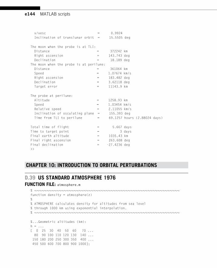
e144 MATLAB scripts
v/vesc = 0.9924
Inclination of translunar orbit = 15.5505 deg
The moon when the probe is at TLI:
Distance = 372242 km
Right ascension = 143.743 deg
Declination = 18.189 deg
The moon when the probe is at perilune:
Distance = 361064 km
Speed = 1.07674 km/s
Right ascension = 183.482 deg
Declination = 3.62118 deg
Target error = 11143.9 km
The probe at perilune:
Altitude = 1258.93 km
Speed = 1.03454 km/s
Relative speed = 2.11055 km/s
Inclination of osculating plane = 155.393 deg
Time from TLI to perilune = 69.1257 hours (2.88024 days)
Total time of flight = 5.667 days
Time to target point = 3 days
Final earth altitude = 1035.43 km
Final right ascension = 263.608 deg
Final declination = -27.4236 deg
>>
CHAPTER 10: INTRODUCTION TO ORBITAL PERTURBATIONS
D.39 US STANDARD ATMOSPHERE 1976FUNCTION FILE: atmosphere.m
% �����������������������������������������������������������function density = atmosphere(z)
%
% ATMOSPHERE calculates density for altitudes from sea level
% through 1000 km using exponential interpolation.
% �����������������������������������������������������������
%...Geometric altitudes (km):
h = ...
[ 0 25 30 40 50 60 70 ...
80 90 100 110 120 130 140 ...
150 180 200 250 300 350 400 ...
450 500 600 700 800 900 1000];
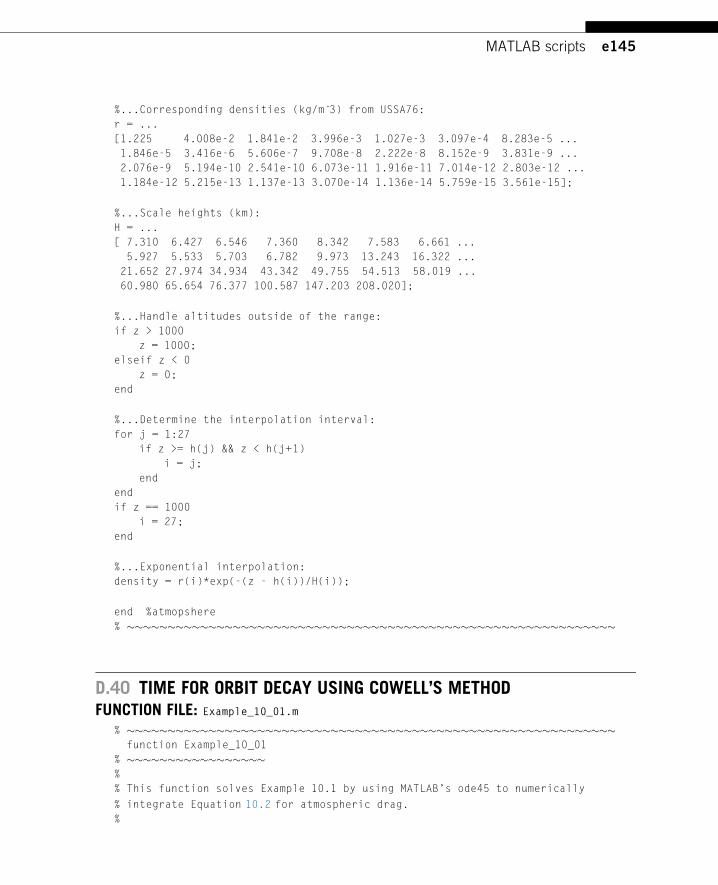
e145MATLAB scripts
%...Corresponding densities (kg/m 3̂) from USSA76:
r = ...
[1.225 4.008e-2 1.841e-2 3.996e-3 1.027e-3 3.097e-4 8.283e-5 ...
1.846e-5 3.416e-6 5.606e-7 9.708e-8 2.222e-8 8.152e-9 3.831e-9 ...
2.076e-9 5.194e-10 2.541e-10 6.073e-11 1.916e-11 7.014e-12 2.803e-12 ...
1.184e-12 5.215e-13 1.137e-13 3.070e-14 1.136e-14 5.759e-15 3.561e-15];
%...Scale heights (km):
H = ...
[ 7.310 6.427 6.546 7.360 8.342 7.583 6.661 ...
5.927 5.533 5.703 6.782 9.973 13.243 16.322 ...
21.652 27.974 34.934 43.342 49.755 54.513 58.019 ...
60.980 65.654 76.377 100.587 147.203 208.020];
%...Handle altitudes outside of the range:
if z > 1000
z = 1000;
elseif z < 0
z = 0;
end
%...Determine the interpolation interval:
for j = 1:27
if z >= h(j) && z < h(j+1)
i = j;
end
end
if z == 1000
i = 27;
end
%...Exponential interpolation:
density = r(i)*exp(-(z - h(i))/H(i));
end %atmopshere
% ������������������������������������������������������������
D.40 TIME FOR ORBIT DECAY USING COWELL’S METHODFUNCTION FILE: Example_10_01.m
% ������������������������������������������������������������function Example_10_01
% �����������������%
% This function solves Example 10.1 by using MATLAB’s ode45 to numerically
% integrate Equation 10.2 for atmospheric drag.
%
e146 MATLAB scripts
% User M-functions required: sv_from_coe, atmosphere
% User subfunctions required: rates, terminate
% –––––––––––––––––––––––––––––––––––––––––––––––––––––––––––––––––––––––––––––
%...Preliminaries:
close all, clear all, clc
%...Conversion factors:
hours = 3600; %Hours to seconds
days = 24*hours; %Days to seconds
deg = pi/180; %Degrees to radians
%...Constants;
mu = 398600; %Gravitational parameter (km 3̂/s 2̂)
RE = 6378; %Earth’s radius (km)
wE = [ 0 0 7.2921159e-5]’; %Earth’s angular velocity (rad/s)
%...Satellite data:
CD = 2.2; %Drag codfficient
m = 100; %Mass (kg)
A = pi/4*(1 2̂) ; %Frontal area (m 2̂)
%...Initial orbital parameters (given):
rp = RE + 215; %perigee radius (km)
ra = RE + 939; %apogee radius (km)
RA = 339.94*deg; %Right ascencion of the node (radians)
i = 65.1*deg; %Inclination (radians)
w = 58*deg; %Argument of perigee (radians)
TA = 332*deg; %True anomaly (radians)
%...Initial orbital parameters (inferred):
e = (ra-rp)/(ra+rp); %eccentricity
a = (rp + ra)/2; %Semimajor axis (km)
h = sqrt(mu*a*(1-e 2̂)); %angular momentrum (km 2̂/s)
T = 2*pi/sqrt(mu)*a 1̂.5; %Period (s)
%...Store initial orbital elements (from above) in the vector coe0:
coe0 = [h e RA i w TA];
%...Obtain the initial state vector from Algorithm 4.5 (sv_from_coe):
[R0 V0] = sv_from_coe(coe0, mu); %R0 is the initial position vector
%V0 is the initial velocity vector
r0 = norm(R0); v0 = norm(V0); %Magnitudes of R0 and V0
%...Use ODE45 to integrate the equations of motion d/dt(R,V) = f(R,V)
% from t0 to tf:
t0 = 0; tf = 120*days; %Initial and final times (s)
e147MATLAB scripts
y0 = [R0 V0]’; %Initial state vector
nout = 40000; %Number of solution points to output
tspan = linspace(t0, tf, nout); %Integration time interval
% Set error tolerances, initial step size, and termination event:
options = odeset(’reltol’, 1.e-8, ...
’abstol’, 1.e-8, ...
’initialstep’, T/10000, ...
’events’, @terminate);
global alt %Altitude
[t,y] = ode45(@rates, tspan, y0,options); %t is the solution times
%y is the state vector history
%...Extract the locally extreme altitudes:
altitude = sqrt(sum(y(:,1:3). 2̂,2)) - RE; %Altitude at each time
[max_altitude,imax,min_altitude,imin] = extrema(altitude);
maxima = [t(imax) max_altitude]; %Maximum altitudes and times
minima = [t(imin) min_altitude]; %Minimum altitudes and times
apogee = sortrows(maxima,1); %Maxima sorted with time
perigee = sortrows(minima,1); %Minima sorted with time
figure(1)
apogee(1,2) = NaN;
%...Plot perigee and apogee history on the same figure:
plot(apogee(:,1)/days, apogee(:,2),’b’,’linewidth’,2)
hold on
plot(perigee(:,1)/days, perigee(:,2),’r’,’linewidth’,2)
grid on
grid minor
xlabel(’Time (days)’)
ylabel(’Altitude (km)’)
ylim([0 1000]);
%...Subfunctions:
% ������������������������������������������������������������function dfdt = rates(t,f)
% ��������������������%
% This function calculates the spacecraft acceleration from its
% position and velocity at time t.
% ––––––––––––––––––––––––––––––––––––––––––––––––––––––––––––––––––––––––
R = f(1:3)’; %Position vector (km/s)
r = norm(R); %Distance from earth’s center (km)
alt = r - RE; %Altitude (km)
rho = atmosphere(alt); %Air density from US Standard Model (kf/m 3̂)
V = f(4:6)’; %Velocity vector (km/s)
Vrel = V - cross(wE,R); %Velocity relative to the atmosphere (km/s)
e148 MATLAB scripts
vrel = norm(Vrel); %Speed relative to the atmosphere (km/s)
uv = Vrel/vrel; %Relative velocity unit vector
ap = -CD*A/m*rho*... %Acceleration due to drag (m/s 2̂)
(1000*vrel) 2̂/2*uv; %(converting units of vrel from km/s to m/s)
a0 = -mu*R/r 3̂; %Gravitational ecceleration (km/s 2̂)
a = a0 + ap/1000; %Total acceleration (km/s 2̂)
dfdt = [V a]’; %Velocity and the acceleraion returned to ode45
end %rates
% ������������������������������������������������������������
% ������������������������������������������������������������function [lookfor stop direction] = terminate(t,y)
% ���������������������������������������%
% This function specifies the event at which ode45 terminates.
% ––––––––––––––––––––––––––––––––––––––––––––––––––––––––––––––––––––––––
lookfor = alt - 100; % = 0 when altitude = 100 km
stop = 1; % 1 means terminate at lookfor = 0; Otherwise 0
direction = -1; % -1 means zero crossing is from above
end %terminate
% ������������������������������������������������������������
end %Example_10_01
% ������������������������������������������������������������
D.41 J2 PERTURBATION OF AN ORBIT USING ENCKE’S METHODFUNCTION FILE: Example_10_02.m
% ������������������������������������������������������������function Example_10_02
% ����������������%
% This function solves Example 10.2 by using Encke’s method together
% with MATLAB’s ode45 to integrate Equation 10.2 for a J2 gravitational
% perturbation given by Equation 10.30.
%
% User M-functions required: sv_from_coe, coe_from_sv, rv_from_r0v0
% User subfunction required: rates
% ––––––––––––––––––––––––––––––––––––––––––––––––––––––––––––––––––––––––
%...Preliminaries:
clc, close all, clear all
%...Conversion factors:
hours = 3600; %Hours to seconds
days = 24*hours; %Days to seconds
deg = pi/180; %Degrees to radians
e149MATLAB scripts
%...Constants:
global mu
mu = 398600; %Gravitational parameter (km 3̂/s 2̂)
RE = 6378; %Earth’s radius (km)
J2 = 1082.63e-6;
%...Initial orbital parameters (given):
zp0 = 300; %Perigee altitude (km)
za0 = 3062; %Apogee altitude (km)
RA0 = 45*deg; %Right ascension of the node (radians)
i0 = 28*deg; %Inclination (radians)
w0 = 30*deg; %Argument of perigee (radians)
TA0 = 40*deg; %True anomaly (radians)
%...Initial orbital parameters (inferred):
rp0 = RE + zp0; %Perigee radius (km)
ra0 = RE + za0; %Apogee radius (km)
e0 = (ra0 - rp0)/(ra0 + rp0); %Eccentricity
a0 = (ra0 + rp0)/2; %Semimajor axis (km)
h0 = sqrt(rp0*mu*(1+e0)); %Angular momentum (km 2̂/s)
T0 = 2*pi/sqrt(mu)*a0 1̂.5; %Period (s)
t0 = 0; tf = 2*days; %Initial and final time (s)
%...end Input data
%Store the initial orbital elements in the array coe0:
coe0 = [h0 e0 RA0 i0 w0 TA0];
%...Obtain the initial state vector from Algorithm 4.5 (sv_from_coe):
[R0 V0] = sv_from_coe(coe0, mu); %R0 is the initial position vector
%R0 is the initial position vector
r0 = norm(R0); v0 = norm(V0); %Magnitudes of T0 and V0
del_t = T0/100; %Time step for Encke procedure
options = odeset(’maxstep’, del_t);
%...Begin the Encke integration;
t = t0; %Initialize the time scalar
tsave = t0; %Initialize the vector of solution times
y = [R0 V0]; %Initialize the state vector
del_y0 = zeros(6,1); %Initialize the state vector perturbation
t = t + del_t; %First time step
% Loop over the time interval [t0, tf] with equal increments del_t:
while t <= tf + del_t/2
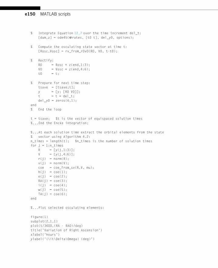
e150 MATLAB scripts
% Integrate Equation 12.7 over the time increment del_t:
[dum,z] = ode45(@rates, [t0 t], del_y0, options);
% Compute the osculating state vector at time t:
[Rosc,Vosc] = rv_from_r0v0(R0, V0, t-t0);
% Rectify:
R0 = Rosc + z(end,1:3);
V0 = Vosc + z(end,4:6);
t0 = t;
% Prepare for next time step:
tsave = [tsave;t];
y = [y; [R0 V0]];
t = t + del_t;
del_y0 = zeros(6,1);
end
% End the loop
t = tsave; %t is the vector of equispaced solution times
%...End the Encke integration;
%...At each solution time extract the orbital elements from the state
% vector using Algorithm 4.2:
n_times = length(t); %n_times is the number of solution times
for j = 1:n_times
R = [y(j,1:3)];
V = [y(j,4:6)];
r(j) = norm(R);
v(j) = norm(V);
coe = coe_from_sv(R,V, mu);
h(j) = coe(1);
e(j) = coe(2);
RA(j) = coe(3);
i(j) = coe(4);
w(j) = coe(5);
TA(j) = coe(6);
end
%...Plot selected osculating elements:
figure(1)
subplot(2,1,1)
plot(t/3600,(RA - RA0)/deg)
title(’Variation of Right Ascension’)
xlabel(’hours’)
ylabel(’{\it\Delta\Omega} (deg)’)
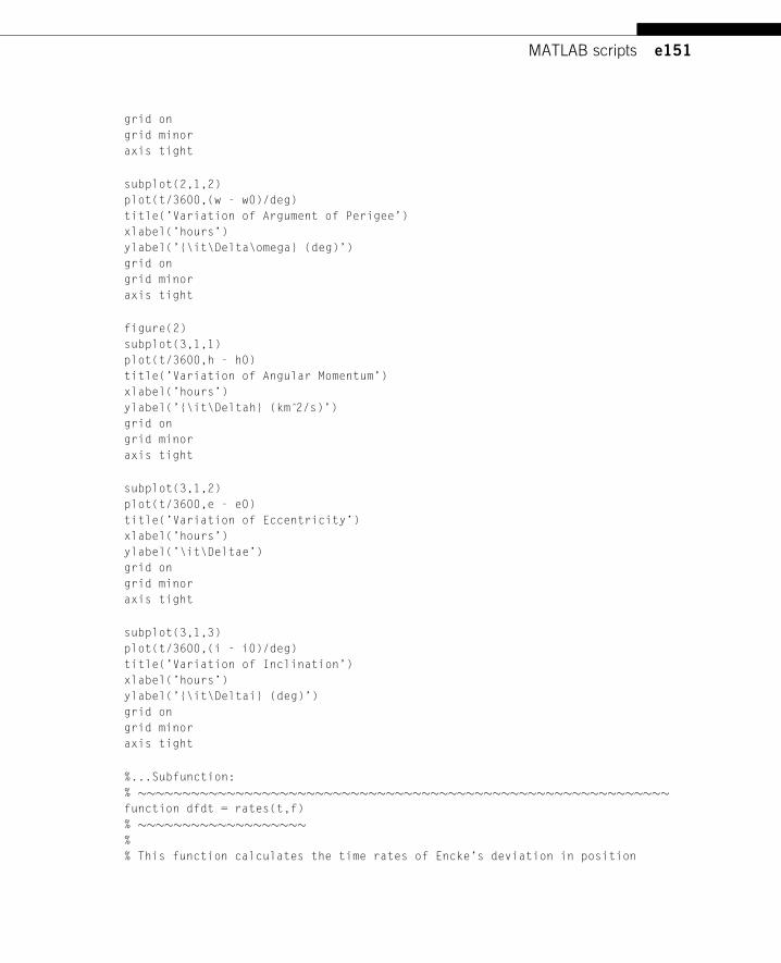
e151MATLAB scripts
grid on
grid minor
axis tight
subplot(2,1,2)
plot(t/3600,(w - w0)/deg)
title(’Variation of Argument of Perigee’)
xlabel(’hours’)
ylabel(’{\it\Delta\omega} (deg)’)
grid on
grid minor
axis tight
figure(2)
subplot(3,1,1)
plot(t/3600,h - h0)
title(’Variation of Angular Momentum’)
xlabel(’hours’)
ylabel(’{\it\Deltah} (km 2̂/s)’)
grid on
grid minor
axis tight
subplot(3,1,2)
plot(t/3600,e - e0)
title(’Variation of Eccentricity’)
xlabel(’hours’)
ylabel(’\it\Deltae’)
grid on
grid minor
axis tight
subplot(3,1,3)
plot(t/3600,(i - i0)/deg)
title(’Variation of Inclination’)
xlabel(’hours’)
ylabel(’{\it\Deltai} (deg)’)
grid on
grid minor
axis tight
%...Subfunction:
% ������������������������������������������������������������function dfdt = rates(t,f)
% �������������������%
% This function calculates the time rates of Encke’s deviation in position
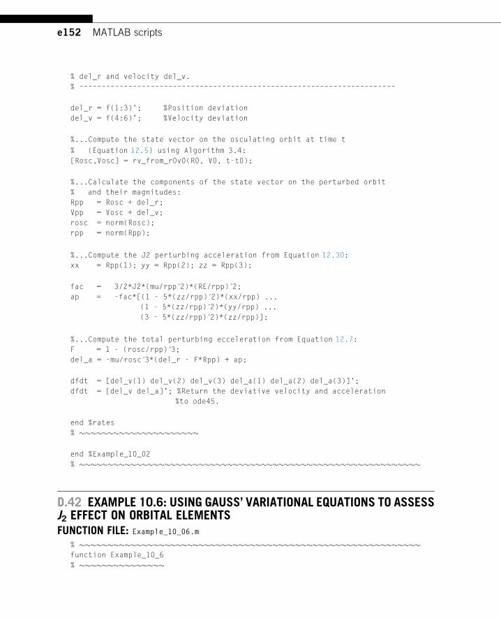
e152 MATLAB scripts
% del_r and velocity del_v.
% –––––––––––––––––––––––––––––––––––––––––––––––––––––––––––––––––––––––
del_r = f(1:3)’; %Position deviation
del_v = f(4:6)’; %Velocity deviation
%...Compute the state vector on the osculating orbit at time t
% (Equation 12.5) using Algorithm 3.4:
[Rosc,Vosc] = rv_from_r0v0(R0, V0, t-t0);
%...Calculate the components of the state vector on the perturbed orbit
% and their magnitudes:
Rpp = Rosc + del_r;
Vpp = Vosc + del_v;
rosc = norm(Rosc);
rpp = norm(Rpp);
%...Compute the J2 perturbing acceleration from Equation 12.30:
xx = Rpp(1); yy = Rpp(2); zz = Rpp(3);
fac = 3/2*J2*(mu/rpp 2̂)*(RE/rpp) 2̂;
ap = -fac*[(1 - 5*(zz/rpp) 2̂)*(xx/rpp) ...
(1 - 5*(zz/rpp) 2̂)*(yy/rpp) ...
(3 - 5*(zz/rpp) 2̂)*(zz/rpp)];
%...Compute the total perturbing ecceleration from Equation 12.7:
F = 1 - (rosc/rpp) 3̂;
del_a = -mu/rosc 3̂*(del_r - F*Rpp) + ap;
dfdt = [del_v(1) del_v(2) del_v(3) del_a(1) del_a(2) del_a(3)]’;
dfdt = [del_v del_a]’; %Return the deviative velocity and acceleration
%to ode45.
end %rates
% ���������������������
end %Example_10_02
% ������������������������������������������������������������
D.42 EXAMPLE 10.6: USING GAUSS’ VARIATIONAL EQUATIONS TO ASSESSJ2 EFFECT ON ORBITAL ELEMENTSFUNCTION FILE: Example_10_06.m
% ������������������������������������������������������������function Example_10_6
% ���������������
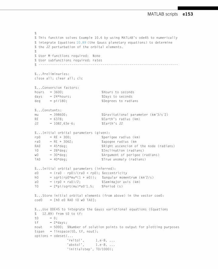
e153MATLAB scripts
%
% This function solves Example 10.6 by using MATLAB’s ode45 to numerically
% integrate Equations 10.89 (the Gauss planetary equations) to determine
% the J2 perturbation of the orbital elements.
%
% User M-functions required: None
% User subfunctions required: rates
% ––––––––––––––––––––––––––––––––––––––––––––––––––––––––––––––––––––––––
%...Preliminaries:
close all; clear all; clc
%...Conversion factors:
hours = 3600; %Hours to seconds
days = 24*hours; %Days to seconds
deg = pi/180; %Degrees to radians
%...Constants:
mu = 398600; %Gravitational parameter (km 3̂/s 2̂)
RE = 6378; %Earth’s radius (km)
J2 = 1082.63e-6; %Earth’s J2
%...Initial orbital parameters (given):
rp0 = RE + 300; %perigee radius (km)
ra0 = RE + 3062; %apogee radius (km
RA0 = 45*deg; %Right ascencion of the node (radians)
i0 = 28*deg; %Inclination (radians)
w0 = 30*deg; %Argument of perigee (radians)
TA0 = 40*deg; %True anomaly (radians)
%...Initial orbital parameters (inferred):
e0 = (ra0 - rp0)/(ra0 + rp0); %eccentricity
h0 = sqrt(rp0*mu*(1 + e0)); %angular momentrum (km 2̂/s)
a0 = (rp0 + ra0)/2; %Semimajor axis (km)
T0 = 2*pi/sqrt(mu)*a0 1̂.5; %Period (s)
%...Store initial orbital elements (from above) in the vector coe0:
coe0 = [h0 e0 RA0 i0 w0 TA0];
%...Use ODE45 to integrate the Gauss variational equations (Equations
% 12.89) from t0 to tf:
t0 = 0;
tf = 2*days;
nout = 5000; %Number of solution points to output for plotting purposes
tspan = linspace(t0, tf, nout);
options = odeset(...
’reltol’, 1.e-8, ...
’abstol’, 1.e-8, ...
’initialstep’, T0/1000);
e154 MATLAB scripts
y0 = coe0’;
[t,y] = ode45(@rates, tspan, y0, options);
%...Assign the time histories mnemonic variable names:
h = y(:,1);
e = y(:,2);
RA = y(:,3);
i = y(:,4);
w = y(:,5);
TA = y(:,6);
%...Plot the time histories of the osculatinig elements:
figure(1)
subplot(5,1,1)
plot(t/3600,(RA - RA0)/deg)
title(’Right Ascension (degrees)’)
xlabel(’hours’)
grid on
grid minor
axis tight
subplot(5,1,2)
plot(t/3600,(w - w0)/deg)
title(’Argument of Perigee (degrees)’)
xlabel(’hours’)
grid on
grid minor
axis tight
subplot(5,1,3)
plot(t/3600,h - h0)
title(’Angular Momentum (km 2̂/s)’)
xlabel(’hours’)
grid on
grid minor
axis tight
subplot(5,1,4)
plot(t/3600,e - e0)
title(’Eccentricity’)
xlabel(’hours’)
grid on
grid minor
axis tight
e155MATLAB scripts
subplot(5,1,5)
plot(t/3600,(i - i0)/deg)
title(’Inclination (degrees)’)
xlabel(’hours’)
grid on
grid minor
axis tight
%...Subfunction:
% ���������������������������������������������������function dfdt = rates(t,f)
% �������������������%
% This function calculates the time rates of the orbital elements
% from Gauss’s variational equations (Equations 12.89).
% –––––––––––––––––––––––––––––––––––––––––––––––––––––––––––––––––––––––––
%...The orbital elements at time t:
h = f(1);
e = f(2);
RA = f(3);
i = f(4);
w = f(5);
TA = f(6);
r = h 2̂/mu/(1 + e*cos(TA)); %The radius
u = w + TA; %Argument of latitude
%...Orbital element rates at time t (Equations 12.89):
hdot = -3/2*J2*mu*RE 2̂/r 3̂*sin(i) 2̂*sin(2*u);
edot = ...
3/2*J2*mu*RE 2̂/h/r 3̂*(h 2̂/mu/r ...
*(sin(u)*sin(i) 2̂*(3*sin(TA)*sin(u) - 2*cos(TA)*cos(u)) - sin(TA)) ...
-sin(i) 2̂*sin(2*u)*(e + cos(TA)));
edot = 3/2*J2*mu*RE 2̂/h/r 3̂ ...
*(h 2̂/mu/r*sin(TA)*(3*sin(i) 2̂*sin(u) 2̂ - 1) ...
-sin(2*u)*sin(i) 2̂*((2+e*cos(TA))*cos(TA)+e));
TAdot = h/r 2̂ + 3/2*J2*mu*RE 2̂/e/h/r 3̂ ...
*(h 2̂/mu/r*cos(TA)*(3*sin(i) 2̂*sin(u) 2̂ - 1) ...
+ sin(2*u)*sin(i) 2̂*sin(TA)*(h 2̂/mu/r + 1));
RAdot = -3*J2*mu*RE 2̂/h/r 3̂*sin(u) 2̂*cos(i);
e156 MATLAB scripts
idot = -3/4*J2*mu*RE 2̂/h/r 3̂*sin(2*u)*sin(2*i);
wdot = 3/2*J2*mu*RE 2̂/e/h/r 3̂ ...
*(-h 2̂/mu/r*cos(TA)*(3*sin(i) 2̂*sin(u) 2̂ - 1) ...
- sin(2*u)*sin(i) 2̂*sin(TA)*(2 + e*cos(TA)) ...
+ 2*e*cos(i) 2̂*sin(u) 2̂);
%...Pass these rates back to ODE45 in the array dfdt:
dfdt = [hdot edot RAdot idot wdot TAdot]’;
end %rates
% ������������������������������������������������������������
end %Example_10_6
% ������������������������������������������������������������
D.43 ALGORITHM 10.2: CALCULATE THE GEOCENTRIC POSITION OF THESUN AT A GIVEN EPOCHFUNCTION FILE: solar_position.m
% ������������������������������������������������������������function [lamda eps r_S] = solar_position(jd)
%
% This function alculates the geocentric equatorial position vector
% of the sun, given the julian date.
%
% User M-functions required: None
% –––––––––––––––––––––––––––––––––––––––––––––––––––––––––––––––––––––––––
%...Astronomical unit (km):
AU = 149597870.691;
%...Julian days since J2000:
n = jd - 2451545;
%...Julian centuries since J2000:
cy = n/36525;
%...Mean anomaly (deg{:
M = 357.528 + 0.9856003*n;
M = mod(M,360);
%...Mean longitude (deg):
L = 280.460 + 0.98564736*n;
L = mod(L,360);
e157MATLAB scripts
%...Apparent ecliptic longitude (deg):
lamda = L + 1.915*sind(M) + 0.020*sind(2*M);
lamda = mod(lamda,360);
%...Obliquity of the ecliptic (deg):
eps = 23.439 - 0.0000004*n;
%...Unit vector from earth to sun:
u = [cosd(lamda); sind(lamda)*cosd(eps); sind(lamda)*sind(eps)];
%...Distance from earth to sun (km):
rS = (1.00014 - 0.01671*cosd(M) - 0.000140*cosd(2*M))*AU;
%...Geocentric position vector (km):
r_S = rS*u;
end %solar_position
% ������������������������������������������������������������
D.44 ALGORITHM 10.3: DETERMINE WHETHER OR NOT A SATELLITE IS INEARTH’S SHADOWFUNCTION FILE: los.m
% ����������������������������������������������������function light_switch = los(r_sat, r_sun)
%
% This function uses the ECI position vectors of the satellite (r_sat)
% and the sun (r_sun) to determine whether the earth is in the line of
% sight between the two.
%
% User M-functions required: None
% –––––––––––––––––––––––––––––––––––––––––––––––––––––––––––––––––––––––––––––
RE = 6378; %Earth’s radius (km)
rsat = norm(r_sat);
rsun = norm(r_sun);
%...Angle between sun and satellite position vectore:
theta = acosd(dot(r_sat, r_sun)/rsat/rsun);
%...Angle between the satellite position vector and the radial to the point
% of tangency with the earth of a line from the satellite:
theta_sat = acosd(RE/rsat);
%...Angle between the sun position vector and the radial to the point
% of tangency with the earth of a line from the sun:
theta_sun = acosd(RE/rsun);
%...Determine whether a line from the sun to the satellite
e158 MATLAB scripts
% intersects the earth:
if theta_sat + theta_sun <= theta
light_switch = 0; %yes
else
light_switch = 1; %no
end
end %los
% ––––––––––––––––––––––––––––––––––––––––––––––––––––––––––––––––––––––––––
D.45 EXAMPLE 10.9: USE GAUSS’ VARIATIONAL EQUATIONS TODETERMINE THE EFFECT OF SOLAR RADIATION PRESSURE ON AN EARTHSATELLITE’S ORBITAL PARAMETERSFUNCTION FILE: Example_10_09.m
% ������������������������������������������������������������function Example_10_09
%
% This function solve Example 10.9 the Gauss planetary equations for
% solar radiation pressure (Equations 10.106).
%
% User M-functions required: sv_from_coe, los, solar_position
% User subfunctions required: rates
% The M-function rsmooth may be found in Garcia, D: “Robust Smoothing of Gridded
Data in One and Higher Dimensions with Missing Values,” Computational Statistics
and Data Analysis, Vol. 54, 1167-1178, 2010.
% ������������������������������������������������������������
global JD %Julian day
%...Preliminaries:
close all
clear all
clc
%...Conversion factors:
hours = 3600; %Hours to seconds
days = 24*hours; %Days to seconds
deg = pi/180; %Degrees to radians
%...Constants;
mu = 398600; %Gravitational parameter (km 3̂/s 2̂)
RE = 6378; %Eath’s radius (km)
c = 2.998e8; %Speed of light (m/s)
S = 1367; %Solar constant (W/m 2̂)
Psr = S/c; %Solar pressure (Pa);
e159MATLAB scripts
%...Satellite data:
CR = 2; %Radiation pressure codfficient
m = 100; %Mass (kg)
As = 200; %Frontal area (m 2̂);
%...Initial orbital parameters (given):
a0 = 10085.44; %Semimajor axis (km)
e0 = 0.025422; %eccentricity
incl0 = 88.3924*deg; %Inclination (radians)
RA0 = 45.38124*deg; %Right ascencion of the node (radians)
TA0 = 343.4268*deg; %True anomaly (radians)
w0 = 227.493*deg; %Argument of perigee (radians)
%...Initial orbital parameters (inferred):
h0 = sqrt(mu*a0*(1-e0 2̂)); %angular momentrum (km 2̂/s)
T0 = 2*pi/sqrt(mu)*a0 1̂.5; %Period (s)
rp0 = h0 2̂/mu/(1 + e0); %perigee radius (km)
ra0 = h0 2̂/mu/(1 - e0); %apogee radius (km)
%...Store initial orbital elements (from above) in the vector coe0:
coe0 = [h0 e0 RA0 incl0 w0 TA0];
%...Use ODE45 to integrate Equations 12.106, the Gauss planetary equations
% from t0 to tf:
JD0 = 2438400.5; %Initial Julian date (6 January 1964 0 UT)
t0 = 0; %Initial time (s)
tf = 3*365*days; %final time (s)
y0 = coe0’; %Initial orbital elements
nout = 4000; %Number of solution points to output
tspan = linspace(t0, tf, nout); %Integration time interval
options = odeset(...
’reltol’, 1.e-8, ...
’abstol’, 1.e-8, ...
’initialstep’, T0/1000);
[t,y] = ode45(@rates, tspan, y0, options);
%...Extract or compute the orbital elements’ time histories from the
% solution vector y:
h = y(:,1);
e = y(:,2);
RA = y(:,3);
incl = y(:,4);
w = y(:,5);
TA = y(:,6);
a = h. 2̂/mu./(1 - e. 2̂);
e160 MATLAB scripts
%...Smooth the data to remove short period variations:
h = rsmooth(h);
e = rsmooth(e);
RA = rsmooth(RA);
incl = rsmooth(incl);
w = rsmooth(w);
a = rsmooth(a);
figure(2)
subplot(3,2,1)
plot(t/days,h - h0)
title(’Angular Momentum (km 2̂/s)’)
xlabel(’days’)
axis tight
subplot(3,2,2)
plot(t/days,e - e0)
title(’Eccentricity’)
xlabel(’days’)
axis tight
subplot(3,2,4)
plot(t/days,(RA - RA0)/deg)
title(’Right Ascension (deg)’)
xlabel(’days’)
axis tight
subplot(3,2,5)
plot(t/days,(incl - incl0)/deg)
title(’Inclination (deg)’)
xlabel(’days’)
axis tight
subplot(3,2,6)
plot(t/days,(w - w0)/deg)
title(’Argument of Perigee (deg)’)
xlabel(’days’)
axis tight
subplot(3,2,3)
plot(t/days,a - a0)
title(’Semimajor axis (km)’)
xlabel(’days’)
axis tight
%...Subfunctions:
% ������������������������������������������������������������
e161MATLAB scripts
function dfdt = rates(t,f)
% �������������������%...Update the Julian Date at time t:
JD = JD0 + t/days;
%...Compoute the apparent position vector of the sun:
[lamda eps r_sun] = solar_position(JD);
%...Convert the ecliptic latitude and the obliquity to radians:
lamda = lamda*deg;
eps = eps*deg;
%...Extract the orbital elements at time t
h = f(1);
e = f(2);
RA = f(3);
i = f(4);
w = f(5);
TA = f(6);
u = w + TA; %Argument of latitude
%...Compute the state vector at time t:
coe = [h e RA i w TA];
[R, V] = sv_from_coe(coe,mu);
%...Calculate the manitude of the radius vector:
r = norm(R);
%...Compute the shadow function and the solar radiation perturbation:
nu = los(R, r_sun);
pSR = nu*(S/c)*CR*As/m/1000;
%...Calculate the trig functions in Equations 12.105.
sl = sin(lamda); cl = cos(lamda);
se = sin(eps); ce = cos(eps);
sW = sin(RA); cW = cos(RA);
si = sin(i); ci = cos(i);
su = sin(u); cu = cos(u);
sT = sin(TA); cT = cos(TA);
%...Calculate the earth-sun unit vector components (Equations 12.105):
ur = sl*ce*cW*ci*su + sl*ce*sW*cu - cl*sW*ci*su ...
+ cl*cW*cu + sl*se*si*su;
us = sl*ce*cW*ci*cu - sl*ce*sW*su - cl*sW*ci*cu ...
- cl*cW*su + sl*se*si*cu;
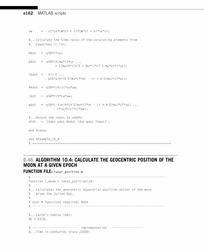
e162 MATLAB scripts
uw = - sl*ce*cW*si + cl*sW*si + sl*se*ci;
%...Calculate the time rates of the osculating elements from
% Equations 12.106:
hdot = -pSR*r*us;
edot = -pSR*(h/mu*sT*ur ...
+ 1/mu/h*((h 2̂ + mu*r)*cT + mu*e*r)*us);
TAdot = h/r 2̂ ...
- pSR/e/h*(h 2̂/mu*cT*ur - (r + h 2̂/mu)*sT*us);
RAdot = -pSR*r/h/si*su*uw;
idot = -pSR*r/h*cu*uw;
wdot = -pSR*(-1/e/h*(h 2̂/mu*cT*ur - (r + h 2̂/mu)*sT*us) ...
- r*su/h/si*ci*uw);
%...Return the rates to ode45:
dfdt = [hdot edot RAdot idot wdot TAdot]’;
end %rates
end %Example_10_9
% ������������������������������������������������������������
D.46 ALGORITHM 10.4: CALCULATE THE GEOCENTRIC POSITION OF THEMOON AT A GIVEN EPOCHFUNCTION FILE: lunar_position.m
% –––––––––––––––––––––––––––––––––––––––––––––––––––––––––––––––––––––––––
function r_moon = lunar_position(jd)
%
%...Calculates the geocentric equatorial position vector of the moon
% given the Julian day.
%
% User M-functions required: None
% –––––––––––––––––––––––––––––––––––––––––––––––––––––––––––––––––––––––––
%...Earth’s radius (km):
RE = 6378;
% ––––––––––––––––––––––––– implementation –––––––––––––––––
%...Time in centuries since J2000:
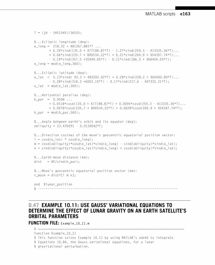
e163MATLAB scripts
T = (jd - 2451545)/36525;
%...Ecliptic longitude (deg):
e_long = 218.32 + 481267.881*T ...
+ 6.29*sind(135.0 + 477198.87*T) - 1.27*sind(259.3 - 413335.36*T)...
+ 0.66*sind(235.7 + 890534.22*T) + 0.21*sind(269.9 + 954397.74*T)...
- 0.19*sind(357.5 +35999.05*T) - 0.11*sind(186.5 + 966404.03*T);
e_long = mod(e_long,360);
%...Ecliptic latitude (deg):
e_lat = 5.13*sind( 93.3 + 483202.02*T) + 0.28*sind(228.2 + 960400.89*T)...
- 0.28*sind(318.3 +6003.15*T) - 0.17*sind(217.6 - 407332.21*T);
e_lat = mod(e_lat,360);
%...Horizontal parallax (deg):
h_par = 0.9508 ...
+ 0.0518*cosd(135.0 + 477198.87*T) + 0.0095*cosd(259.3 - 413335.36*T)...
+ 0.0078*cosd(235.7 + 890534.22*T) + 0.0028*cosd(269.9 + 954397.74*T);
h_par = mod(h_par,360);
%...Angle between earth’s orbit and its equator (deg):
obliquity = 23.439291 - 0.0130042*T;
%...Direction cosines of the moon’s geocentric equatorial position vector:
l = cosd(e_lat) * cosd(e_long);
m = cosd(obliquity)*cosd(e_lat)*sind(e_long) - sind(obliquity)*sind(e_lat);
n = sind(obliquity)*cosd(e_lat)*sind(e_long) + cosd(obliquity)*sind(e_lat);
%...Earth-moon distance (km):
dist = RE/sind(h_par);
%...Moon’s geocentric equatorial position vector (km):
r_moon = dist*[l m n];
end %lunar_position
% –––––––––––––––––––––––––––––––––––––––––––––––––––––––––––––––––––––––––
D.47 EXAMPLE 10.11: USE GAUSS’ VARIATIONAL EQUATIONS TODETERMINE THE EFFECT OF LUNAR GRAVITY ON AN EARTH SATELLITE’SORBITAL PARAMETERSFUNCTION FILE: Example_10_11.m
% ������������������������������������������������������������function Example_10_11
% This function solves Example 10.11 by using MATLAB’s ode45 to integrate
% Equations 10.84, the Gauss variational equations, for a lunar
% gravitational perturbation.
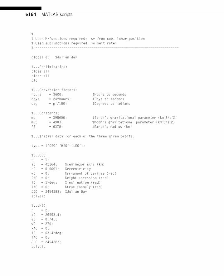
e164 MATLAB scripts
%
% User M-functions required: sv_from_coe, lunar_position
% User subfunctions required: solveit rates
% ––––––––––––––––––––––––––––––––––––––––––––––––––––––––––––––––––––––––
global JD %Julian day
%...Preliminaries:
close all
clear all
clc
%...Conversion factors:
hours = 3600; %Hours to seconds
days = 24*hours; %Days to seconds
deg = pi/180; %Degrees to radians
%...Constants;
mu = 398600; %Earth’s gravitational parameter (km 3̂/s 2̂)
mu3 = 4903; %Moon’s gravitational parameter (km 3̂/s 2̂)
RE = 6378; %Earth’s radius (km)
%...Initial data for each of the three given orbits:
type = {’GEO’ ’HEO’ ’LEO’};
%...GEO
n = 1;
a0 = 42164; %semimajor axis (km)
e0 = 0.0001; %eccentricity
w0 = 0; %argument of perigee (rad)
RA0 = 0; %right ascension (rad)
i0 = 1*deg; %inclination (rad)
TA0 = 0; %true anomaly (rad)
JD0 = 2454283; %Julian Day
solveit
%...HEO
n = 2;
a0 = 26553.4;
e0 = 0.741;
w0 = 270;
RA0 = 0;
i0 = 63.4*deg;
TA0 = 0;
JD0 = 2454283;
solveit
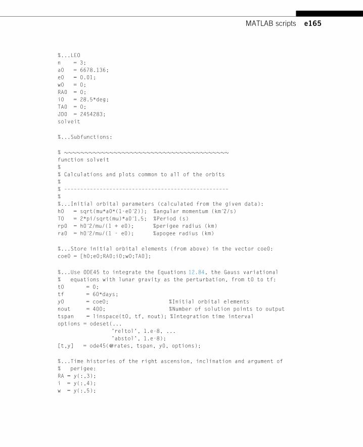
e165MATLAB scripts
%...LEO
n = 3;
a0 = 6678.136;
e0 = 0.01;
w0 = 0;
RA0 = 0;
i0 = 28.5*deg;
TA0 = 0;
JD0 = 2454283;
solveit
%...Subfunctions:
% ����������������������������������������function solveit
%
% Calculations and plots common to all of the orbits
%
% –––––––––––––––––––––––––––––––––––––––––––––––––––
%
%...Initial orbital parameters (calculated from the given data):
h0 = sqrt(mu*a0*(1-e0 2̂)); %angular momentum (km 2̂/s)
T0 = 2*pi/sqrt(mu)*a0 1̂.5; %Period (s)
rp0 = h0 2̂/mu/(1 + e0); %perigee radius (km)
ra0 = h0 2̂/mu/(1 - e0); %apogee radius (km)
%...Store initial orbital elements (from above) in the vector coe0:
coe0 = [h0;e0;RA0;i0;w0;TA0];
%...Use ODE45 to integrate the Equations 12.84, the Gauss variational
% equations with lunar gravity as the perturbation, from t0 to tf:
t0 = 0;
tf = 60*days;
y0 = coe0; %Initial orbital elements
nout = 400; %Number of solution points to output
tspan = linspace(t0, tf, nout); %Integration time interval
options = odeset(...
’reltol’, 1.e-8, ...
’abstol’, 1.e-8);
[t,y] = ode45(@rates, tspan, y0, options);
%...Time histories of the right ascension, inclination and argument of
% perigee:
RA = y(:,3);
i = y(:,4);
w = y(:,5);
e166 MATLAB scripts
%...Smooth the data to eliminate short period variations:
RA = rsmooth(RA);
i = rsmooth(i);
w = rsmooth(w);
figure(n)
subplot(1,3,1)
plot(t/days,(RA - RA0)/deg)
title(’Right Ascension vs Time’)
xlabel(’{\itt} (days)’)
ylabel(’{\it\Omega} (deg)’)
axis tight
subplot(1,3,2)
plot(t/days,(i - i0)/deg)
title(’Inclination vs Time’)
xlabel(’{\itt} (days)’)
ylabel(’{\iti} (deg)’)
axis tight
subplot(1,3,3)
plot(t/days,(w - w0)/deg)
title(’Argument of Perigee vs Time’)
xlabel(’{\itt} (days)’)
ylabel(’{\it\omega} (deg)’)
axis tight
drawnow
end %solveit
% �������������������
% �������������������function dfdt = rates(t,f)
% �������������������%...The orbital elements at time t:
h = f(1);
e = f(2);
RA = f(3);
i = f(4);
w = f(5);
TA = f(6);
phi = w + TA; %argument of latitude
%...Obtain the state vector at time t from Algorithm 4.5:
coe = [h e RA i w TA];
[R, V] = sv_from_coe(coe,mu);
e167MATLAB scripts
%...Obtain the unit vectors of the rsw system:
r = norm(R);
ur = R/r; %radial
H = cross(R,V);
uh = H/norm(H); %normal
s = cross(uh, ur);
us = s/norm(s); %transverse
%...Update the Julian Day:
JD = JD0 + t/days;
%...Find and normalize the position vector of the moon:
R_m = lunar_position(JD);
r_m = norm(R_m);
R_rel = R_m - R; %R_rel = position vector of moon wrt satellite
r_rel = norm(R_rel);
%...See Appendix F:
q = dot(R,(2*R_m - R))/r_m 2̂;
F = (q 2̂ - 3*q + 3)*q/(1 + (1-q) 1̂.5);
%...Gravitationl perturbation of the moon (Equation 12.117):
ap = mu3/r_rel 3̂*(F*R_m - R);
%...Perturbation components in the rsw system:
apr = dot(ap,ur);
aps = dot(ap,us);
aph = dot(ap,uh);
%...Gauss variational equations (Equations 12.84):
hdot = r*aps;
edot = h/mu*sin(TA)*apr ...
+ 1/mu/h*((h 2̂ + mu*r)*cos(TA) + mu*e*r)*aps;
RAdot = r/h/sin(i)*sin(phi)*aph;
idot = r/h*cos(phi)*aph;
wdot = - h*cos(TA)/mu/e*apr ...
+ (h 2̂ + mu*r)/mu/e/h*sin(TA)*aps ...
- r*sin(phi)/h/tan(i)*aph;
TAdot = h/r 2̂ ...
+ 1/e/h*(h 2̂/mu*cos(TA)*apr - (r + h 2̂/mu)*sin(TA)*aps);
e168 MATLAB scripts
%...Return rates to ode45 in the array dfdt:
dfdt = [hdot edot RAdot idot wdot TAdot]’;
end %rates
% �����������������
end %Example_10_11
% ������������������������������������������������������������
D.48 EXAMPLE 10.12: USE GAUSS’ VARIATIONAL EQUATIONS TODETERMINE THE EFFECT OF SOLAR GRAVITY ON AN EARTH SATELLITE’SORBITAL PARAMETERSFUNCTION FILE: Example_10_12.m
% ������������������������������������������������������������function Example_10_12
% This function solves Example 10.12 by using MATLAB’s ode45 to integrate
% Equations 10.84, the Gauss variational equations, for a solar
% gravitational perturbation.
%
% User M-functions required: sv_from_coe, lunar_position
% User subfunctions required: solveit rates
% ––––––––––––––––––––––––––––––––––––––––––––––––––––––––––––––––––––––––
global JD %Julian day
%...Preliminaries:
close all
clear all
clc
%...Conversion factors:
hours = 3600; %Hours to seconds
days = 24*hours; %Days to seconds
deg = pi/180; %Degrees to radians
%...Constants;
mu = 398600; %Earth’s gravitational parameter (km 3̂/s 2̂)
mu3 = 132.712e9; %Sun’s gravitational parameter (km 3̂/s 2̂)
RE = 6378; %Earth’s radius (km)
%...Initial data for each of the three given orbits:
type = {’GEO’ ’HEO’ ’LEO’};
%...GEO
n = 1;
e169MATLAB scripts
a0 = 42164; %semimajor axis (km)
e0 = 0.0001; %eccentricity
w0 = 0; %argument of perigee (rad)
RA0 = 0; %right ascension (rad)
i0 = 1*deg; %inclination (rad)
TA0 = 0; %true anomaly (rad)
JD0 = 2454283; %Julian Day
solveit
%...HEO
n = 2;
a0 = 26553.4;
e0 = 0.741;
w0 = 270;
RA0 = 0;
i0 = 63.4*deg;
TA0 = 0;
JD0 = 2454283;
solveit
%...LEO
n = 3;
a0 = 6678.136;
e0 = 0.01;
w0 = 0;
RA0 = 0;
i0 = 28.5*deg;
TA0 = 0;
JD0 = 2454283;
solveit
%...Subfunctions:
% ����������������������������������������function solveit
%
% Calculations and plots common to all of the orbits
%
% –––––––––––––––––––––––––––––––––––––––––––––––––––
%
%...Initial orbital parameters (calculated from the given data):
h0 = sqrt(mu*a0*(1-e0 2̂)); %angular momentum (km 2̂/s)
T0 = 2*pi/sqrt(mu)*a0 1̂.5; %Period (s)
rp0 = h0 2̂/mu/(1 + e0); %perigee radius (km)
ra0 = h0 2̂/mu/(1 - e0); %apogee radius (km)
%...Store initial orbital elements (from above) in the vector coe0:
coe0 = [h0;e0;RA0;i0;w0;TA0];
e170 MATLAB scripts
%...Use ODE45 to integrate the Equations 12.84, the Gauss variational
% equations with lunar gravity as the perturbation, from t0 to tf:
t0 = 0;
tf = 720*days;
y0 = coe0; %Initial orbital elements
nout = 400; %Number of solution points to output
tspan = linspace(t0, tf, nout); %Integration time interval
options = odeset(...
’reltol’, 1.e-8, ...
’abstol’, 1.e-8);
[t,y] = ode45(@rates, tspan, y0, options);
%...Time histories of the right ascension, inclination and argument of
% perigee:
RA = y(:,3);
i = y(:,4);
w = y(:,5);
%...Smooth the data to eliminate short period variations:
RA = rsmooth(RA);
i = rsmooth(i);
w = rsmooth(w);
figure(n)
subplot(1,3,1)
plot(t/days,(RA - RA0)/deg)
title(’Right Ascension vs Time’)
xlabel(’{\itt} (days)’)
ylabel(’{\it\Omega} (deg)’)
axis tight
subplot(1,3,2)
plot(t/days,(i - i0)/deg)
title(’Inclination vs Time’)
xlabel(’{\itt} (days)’)
ylabel(’{\iti} (deg)’)
axis tight
subplot(1,3,3)
plot(t/days,(w - w0)/deg)
title(’Argument of Perigee vs Time’)
xlabel(’{\itt} (days)’)
ylabel(’{\it\omega} (deg)’)
axis tight
e171MATLAB scripts
drawnow
end %solveit
% �������������������
% �������������������function dfdt = rates(t,f)
% �������������������%...The orbital elements at time t:
h = f(1);
e = f(2);
RA = f(3);
i = f(4);
w = f(5);
TA = f(6);
phi = w + TA; %argument of latitude
%...Obtain the state vector at time t from Algorithm 4.5:
coe = [h e RA i w TA];
[R, V] = sv_from_coe(coe,mu);
%...Obtain the unit vectors of the rsw system:
r = norm(R);
ur = R/r; %radial
H = cross(R,V);
uh = H/norm(H); %normal
s = cross(uh, ur);
us = s/norm(s); %transverse
%...Update the Julian Day:
JD = JD0 + t/days;
%...Find and normalize the position vector of the sun:
[lamda eps R_S] = solar_position(JD);
r_S = norm(R_S);
R_rel = R_S’ - R; %R_rel = position vector of sun wrt satellite
r_rel = norm(R_rel);
%...See Appendix F:
q = dot(R,(2*R_S’ - R))/r_S 2̂;
F = (q 2̂ - 3*q + 3)*q/(1 + (1-q) 1̂.5);;
%...Gravitationl perturbation of the sun (Equation 12.130):
ap = mu3/r_rel 3̂*(F*R_S’ - R);
%...Perturbation components in the rsw system:
apr = dot(ap,ur);
aps = dot(ap,us);
aph = dot(ap,uh);
e172 MATLAB scripts
%...Gauss variational equations (Equations 12.84):
hdot = r*aps;
edot = h/mu*sin(TA)*apr ...
+ 1/mu/h*((h 2̂ + mu*r)*cos(TA) + mu*e*r)*aps;
RAdot = r/h/sin(i)*sin(phi)*aph;
idot = r/h*cos(phi)*aph;
wdot = - h*cos(TA)/mu/e*apr ...
+ (h 2̂ + mu*r)/mu/e/h*sin(TA)*aps ...
- r*sin(phi)/h/tan(i)*aph;
TAdot = h/r 2̂ ...
+ 1/e/h*(h 2̂/mu*cos(TA)*apr - (r + h 2̂/mu)*sin(TA)*aps);
%...Return rates to ode45 in the array dfdt:
dfdt = [hdot edot RAdot idot wdot TAdot]’;
end %rates
% ���������������
end %Example_10_12
% ������������������������������������������������������������
CHAPTER 11: RIGID BODY DYNAMICS
D.49 ALGORITHM 11.1: CALCULATE THE DIRECTION COSINE MATRIX FROMTHE QUATERNIONFUNCTION FILE: dcm_from_q.m
% �����������������������������������function Q = dcm_from_q(q)
% �������������������%{
This function calculates the direction cosine matrix
from the quaternion.
q - quaternion (where q(4) is the scalar part)
Q - direction cosine matrix
%}
% ––––––––––––––––––––––––––––––––––––––––––––––
e173MATLAB scripts
q1 = q(1); q2 = q(2); q3 = q(3); q4 = q(4);
Q = [q1 2̂-q2 2̂-q3 2̂+q4 2̂, 2*(q1*q2+q3*q4), 2*(q1*q3-q2*q4);
2*(q1*q2-q3*q4), -q1 2̂+q2 2̂-q3 2̂+q4 2̂, 2*(q2*q3+q1*q4);
2*(q1*q3+q2*q4), 2*(q2*q3-q1*q4), -q1 2̂-q2 2̂+q3 2̂+q4 2̂ ];
end %dcm_from_q
% �����������������������������������
D.50 ALGORITHM 11.2: CALCULATE THE QUATERNION FROM THEDIRECTION COSINE MATRIXFUNCTION FILE: q_from_dcm.m
% �����������������������������������function q = q_from_dcm(Q)
% �������������������%{
This function calculates the quaternion from the direction
cosine matrix.
Q - direction cosine matrix
q - quaternion (where q(4) is the scalar part)
%}
% ––––––––––––––––––––––––––––––––––––––––––––––
K3 = ...
[Q(1,1)-Q(2,2)-Q(3,3), Q(2,1)+Q(1,2), Q(3,1)+Q(1,3), Q(2,3)-Q(3,2);
Q(2,1)+Q(1,2), Q(2,2)-Q(1,1)-Q(3,3), Q(3,2)+Q(2,3), Q(3,1)-Q(1,3);
Q(3,1)+Q(1,3), Q(3,2)+Q(2,3), Q(3,3)-Q(1,1)-Q(2,2), Q(1,2)-Q(2,1);
Q(2,3)-Q(3,2), Q(3,1)-Q(1,3), Q(1,2)-Q(2,1), Q(1,1)+Q(2,2)+Q(3,3)]/3;
[eigvec, eigval] = eig(K3);
[x,i] = max(diag(eigval));
q = eigvec(:,i);
end %q_from_dcm
% �����������������������������������
D.51 QUATERNION VECTOR ROTATION OPERATION (EQ. 11.160)FUNCTION FILE: quat_rotate.m
% ����������������������������������������function r = quat_rotate(q,v)
% ���������������������
e174 MATLAB scripts
%{
quat_rotate rotates a vector by a unit quaternion.
r = quat_rotate(q,v) calculates the rotated vector r for a
quaternion q and a vector v.
q is a 1-by-4 matrix whose norm must be 1. q(1) is the scalar part
of the quaternion.
v is a 1-by-3 matrix.
r is a 1-by-3 matrix.
The 3-vector v is made into a pure quaternion 4-vector V = [0 v]. r is
produced by the quaternion product R = q*V*qinv. r = [R(2) R(3) R(4)].
MATLAB M-functions used: quatmultiply, quatinv.
%}
% –––––––––––––––––––––––––––––––––––––––––––––––––––
qinv = quatinv(q);
r = quatmultiply(quatmultiply(q,[0 v]),qinv);
r = r(2:4);
end %quat_rotate
% ����������������������������������������
D.52 EXAMPLE 11.26: SOLUTION OF THE SPINNING TOP PROBLEMFUNCTION FILE: Example_11_23.m
% ������������������������function Example_11_26
% ����������������%{
This program numerically integrates Euler’s equations of motion
for the spinning top (Example 11.26, Equations (a)). The
quaternion is used to obtain the time history of the top’s
orientation. See Figures 11.34 and 11.35.
User M-functions required: rkf45, q_from_dcm, dcm_from_q, dcm_to_euler
User subfunction required: rates
%}
% ––––––––––––––––––––––––––––––––––––––––––––––
clear all; close all; clc
%...Data from Example 11.15:
g = 9.807; % Acceleration of gravity (m/s 2̂)
m = 0.5; % Mass in kg
d = 0.05; % Distance of center of mass from pivot point (m)
A = 12.e-4; % Moment of inertia about body x (kg-m 2̂)
B = 12.e-4; % Moment of inertia about body y (kg-m 2̂)
C = 4.5e-4; % Moment of inertia about body z (kg-m 2̂)
e175MATLAB scripts
ws0 = 1000*2*pi/60; % Spin rate (rad/s)
wp0 = 51.93*2*pi/60;% Precession rate (rad/s) Use to obtain Fig. 11.33
wp0 = 0; % Use to obtain Fig, 11.34
wn0 = 0; % Nutation rate (deg/s)
theta = 60; % Initial nutation angle (deg)
z = [0 -sind(theta) cosd(theta)]; % Initial z-axis direction:
p = [1 0 0]; % Initial x-axis direction
% (or a line defining x-z plane)
%...
y = cross(z,p); % y-axis direction (normal to x-z plane)
x = cross(y,z); % x-axis direction (normal to y-z plane)
i = x/norm(x); % Unit vector along x axis
j = y/norm(y); % Unit vector along y axis
k = z/norm(z); % Unit vector along z axis
QXx = [i; j; k]; % Initial direction cosine matrix
%...Initial precession, nutation, and spin angles (deg):
[phi0 theta0 psi0] = dcm_to_euler(QXx);
%...Initial quaternion (column vector):
q0 = q_from_dcm(QXx);
%...Initial body-frame angular velocity, column vector (rad/s):
w0 = [wp0*sind(theta0)*sin(psi0) + wn0*cosd(psi0), ...
wp0*sind(theta0)*cos(psi0) - wn0*sind(psi0), ...
ws0 + wp0*cosd(theta0)]’;
t0 = 0; % Initial time (s)
tf = 1.153; % Final time (s) (for 360 degrees of precession)
f0 = [q0; w0]; % Initial conditions vector (quaternion & angular
% velocities)
%...RKF4(5) numerical ODE solver. Time derivatives computed in
% function ’rates’ below.
[t,f] = rkf45(@rates, [t0,tf], f0);
%...Solutions for quaternion and angular velocities at ’nsteps’ times
% from t0 to tf
q = f(:,1:4);
wx = f(:,5);
wy = f(:,6);
wz = f(:,7);
%...Obtain the direction cosine matrix, the Euler angles and the Euler
% angle rates at each solution time:
e176 MATLAB scripts
for m = 1:length(t)
%...DCM from the quaternion:
QXx = dcm_from_q(q(m,:));
%...Euler angles (deg) from DCM:
[prec(m) ...
nut(m) ...
spin(m)] = dcm_to_euler(QXx);
%...Euler rates from Eqs. 11.116:
wp(m) = (wx(m)*sind(spin(m)) + wy(m)*cosd(spin(m)))/sind(nut(m));
wn(m) = wx(m)*cosd(spin(m)) - wy(m)*sind(spin(m));
ws(m) = -wp(m)*cosd(nut(m)) + wz(m);
end
plotit
% �������������������function dfdt = rates(t,f)
% �������������������q = f(1:4); % components of quaternion
wx = f(5); % angular velocity along x
wy = f(6); % angular velocity along y
wz = f(7); % angular velocity along z
q = q/norm(q); % normalize the quaternion
Q = dcm_from_q(q); % DCM from quaternion
%...Body frame components of the moment of the weight vector
% about the pivot point:
M = Q*[-m*g*d*Q(3,2)
m*g*d*Q(3,1)
0];
%...Skew-symmetric matrix of angular velocities:
Omega = [ 0 wz -wy wx
-wz 0 wx wy
wy -wx 0 wz
-wx -wy -wz 0];
q_dot = Omega*q/2; % time derivative of quaternion
%...Euler’s equations:
wx_dot = M(1)/A - (C - B)*wy*wz/A; % time derivative of wx
wy_dot = M(2)/B - (A - C)*wz*wx/B; % time derivative of wy
wz_dot = M(3)/C - (B - A)*wx*wy/C; % time derivative of wz
%...Return the rates in a column vector:
dfdt = [q_dot; wx_dot; wy_dot; wz_dot];
end %rates
e177MATLAB scripts
% �����������function plotit
% �����������
figure(’Name’, ’Euler angles and their rates’, ’color’, [1 1 1])
subplot(321)
plot(t, prec )
xlabel(’time (s)’)
ylabel(’Precession angle (deg)’)
axis([-inf, inf, -inf, inf])
axis([-inf, inf, -inf, inf])
grid
subplot(322)
plot(t, wp*60/2/pi)
xlabel(’time (s)’)
ylabel(’Precession rate (rpm)’)
axis([0, 1.153, 51, 53])
axis([-inf, inf, -inf, inf])
grid
subplot(323)
plot(t, nut)
xlabel(’time (s)’)
ylabel(’Nutation angle (deg)’)
axis([0, 1.153, 59, 61])
axis([-inf, inf, -inf, inf])
grid
subplot(324)
plot(t, wn*180/pi)
xlabel(’time (s)’)
ylabel(’Nutation rate (deg/s)’)
axis([-inf, inf, -inf, inf])
grid
subplot(325)
plot(t, spin)
xlabel(’time (s)’)
ylabel(’Spin angle (deg)’)
axis([-inf, inf, -inf, inf])
grid
subplot(326)
plot(t, ws*60/2/pi)
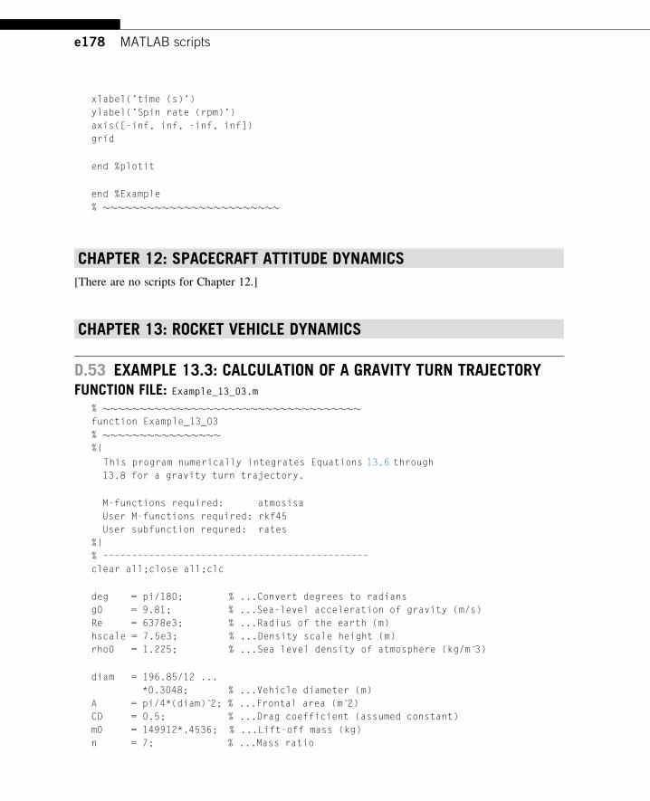
e178 MATLAB scripts
xlabel(’time (s)’)
ylabel(’Spin rate (rpm)’)
axis([-inf, inf, -inf, inf])
grid
end %plotit
end %Example
% ������������������������
CHAPTER 12: SPACECRAFT ATTITUDE DYNAMICS
[There are no scripts for Chapter 12.]
CHAPTER 13: ROCKET VEHICLE DYNAMICS
D.53 EXAMPLE 13.3: CALCULATION OF A GRAVITY TURN TRAJECTORYFUNCTION FILE: Example_13_03.m
% �����������������������������������function Example_13_03
% ����������������%{
This program numerically integrates Equations 13.6 through
13.8 for a gravity turn trajectory.
M-functions required: atmosisa
User M-functions required: rkf45
User subfunction requred: rates
%}
% ––––––––––––––––––––––––––––––––––––––––––––––
clear all;close all;clc
deg = pi/180; % ...Convert degrees to radians
g0 = 9.81; % ...Sea-level acceleration of gravity (m/s)
Re = 6378e3; % ...Radius of the earth (m)
hscale = 7.5e3; % ...Density scale height (m)
rho0 = 1.225; % ...Sea level density of atmosphere (kg/m 3̂)
diam = 196.85/12 ...
*0.3048; % ...Vehicle diameter (m)
A = pi/4*(diam) 2̂; % ...Frontal area (m 2̂)
CD = 0.5; % ...Drag coefficient (assumed constant)
m0 = 149912*.4536; % ...Lift-off mass (kg)
n = 7; % ...Mass ratio
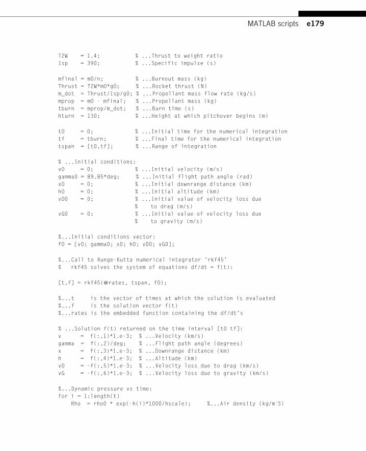
e179MATLAB scripts
T2W = 1.4; % ...Thrust to weight ratio
Isp = 390; % ...Specific impulse (s)
mfinal = m0/n; % ...Burnout mass (kg)
Thrust = T2W*m0*g0; % ...Rocket thrust (N)
m_dot = Thrust/Isp/g0; % ...Propellant mass flow rate (kg/s)
mprop = m0 - mfinal; % ...Propellant mass (kg)
tburn = mprop/m_dot; % ...Burn time (s)
hturn = 130; % ...Height at which pitchover begins (m)
t0 = 0; % ...Initial time for the numerical integration
tf = tburn; % ...Final time for the numerical integration
tspan = [t0,tf]; % ...Range of integration
% ...Initial conditions:
v0 = 0; % ...Initial velocity (m/s)
gamma0 = 89.85*deg; % ...Initial flight path angle (rad)
x0 = 0; % ...Initial downrange distance (km)
h0 = 0; % ...Initial altitude (km)
vD0 = 0; % ...Initial value of velocity loss due
% to drag (m/s)
vG0 = 0; % ...Initial value of velocity loss due
% to gravity (m/s)
%...Initial conditions vector:
f0 = [v0; gamma0; x0; h0; vD0; vG0];
%...Call to Runge-Kutta numerical integrator ’rkf45’
% rkf45 solves the system of equations df/dt = f(t):
[t,f] = rkf45(@rates, tspan, f0);
%...t is the vector of times at which the solution is evaluated
%...f is the solution vector f(t)
%...rates is the embedded function containing the df/dt’s
% ...Solution f(t) returned on the time interval [t0 tf]:
v = f(:,1)*1.e-3; % ...Velocity (km/s)
gamma = f(:,2)/deg; % ...Flight path angle (degrees)
x = f(:,3)*1.e-3; % ...Downrange distance (km)
h = f(:,4)*1.e-3; % ...Altitude (km)
vD = -f(:,5)*1.e-3; % ...Velocity loss due to drag (km/s)
vG = -f(:,6)*1.e-3; % ...Velocity loss due to gravity (km/s)
%...Dynamic pressure vs time:
for i = 1:length(t)
Rho = rho0 * exp(-h(i)*1000/hscale); %...Air density (kg/m 3̂)
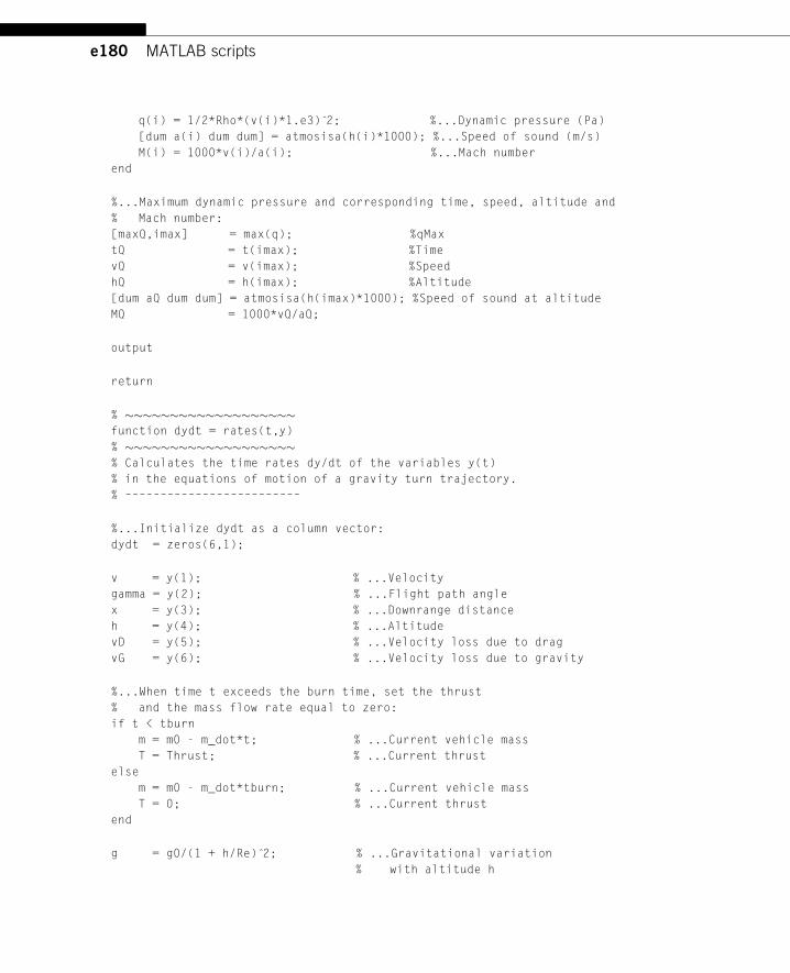
e180 MATLAB scripts
q(i) = 1/2*Rho*(v(i)*1.e3) 2̂; %...Dynamic pressure (Pa)
[dum a(i) dum dum] = atmosisa(h(i)*1000); %...Speed of sound (m/s)
M(i) = 1000*v(i)/a(i); %...Mach number
end
%...Maximum dynamic pressure and corresponding time, speed, altitude and
% Mach number:
[maxQ,imax] = max(q); %qMax
tQ = t(imax); %Time
vQ = v(imax); %Speed
hQ = h(imax); %Altitude
[dum aQ dum dum] = atmosisa(h(imax)*1000); %Speed of sound at altitude
MQ = 1000*vQ/aQ;
output
return
% �������������������function dydt = rates(t,y)
% �������������������% Calculates the time rates dy/dt of the variables y(t)
% in the equations of motion of a gravity turn trajectory.
% –––––––––––––––––––––––––
%...Initialize dydt as a column vector:
dydt = zeros(6,1);
v = y(1); % ...Velocity
gamma = y(2); % ...Flight path angle
x = y(3); % ...Downrange distance
h = y(4); % ...Altitude
vD = y(5); % ...Velocity loss due to drag
vG = y(6); % ...Velocity loss due to gravity
%...When time t exceeds the burn time, set the thrust
% and the mass flow rate equal to zero:
if t < tburn
m = m0 - m_dot*t; % ...Current vehicle mass
T = Thrust; % ...Current thrust
else
m = m0 - m_dot*tburn; % ...Current vehicle mass
T = 0; % ...Current thrust
end
g = g0/(1 + h/Re) 2̂; % ...Gravitational variation
% with altitude h
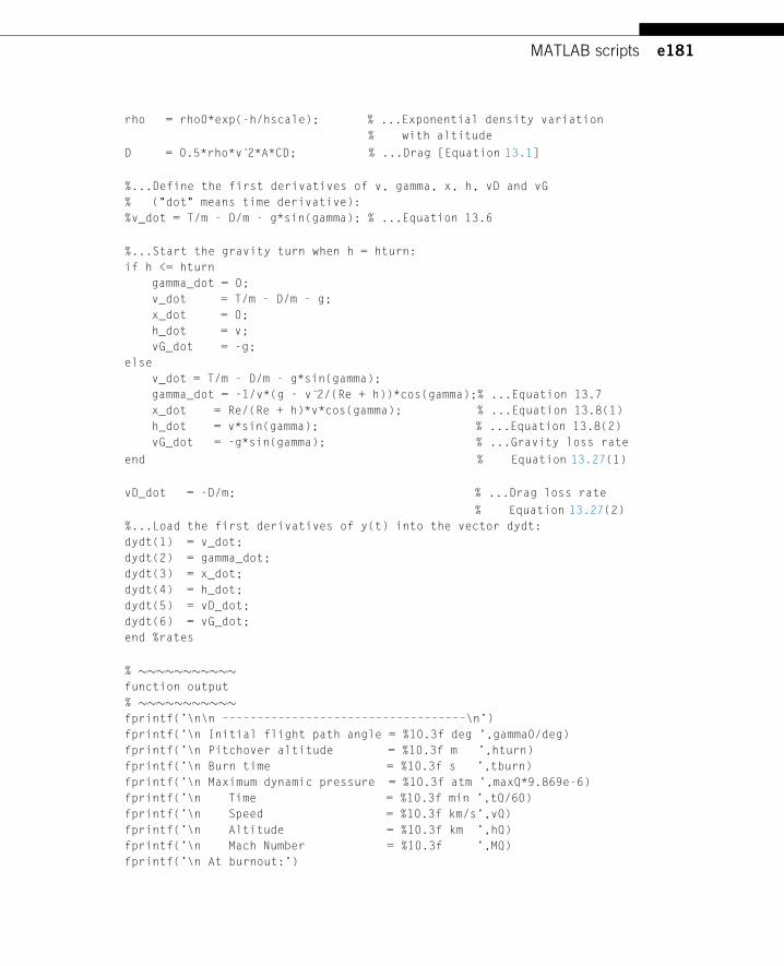
e181MATLAB scripts
rho = rho0*exp(-h/hscale); % ...Exponential density variation
% with altitude
D = 0.5*rho*v 2̂*A*CD; % ...Drag [Equation 13.1]
%...Define the first derivatives of v, gamma, x, h, vD and vG
% ("dot" means time derivative):
%v_dot = T/m - D/m - g*sin(gamma); % ...Equation 13.6
%...Start the gravity turn when h = hturn:
if h <= hturn
gamma_dot = 0;
v_dot = T/m - D/m - g;
x_dot = 0;
h_dot = v;
vG_dot = -g;
else
v_dot = T/m - D/m - g*sin(gamma);
gamma_dot = -1/v*(g - v 2̂/(Re + h))*cos(gamma);% ...Equation 13.7
x_dot = Re/(Re + h)*v*cos(gamma); % ...Equation 13.8(1)
h_dot = v*sin(gamma); % ...Equation 13.8(2)
vG_dot = -g*sin(gamma); % ...Gravity loss rate
end % Equation 13.27(1)
vD_dot = -D/m; % ...Drag loss rate
% Equation 13.27(2)
%...Load the first derivatives of y(t) into the vector dydt:
dydt(1) = v_dot;
dydt(2) = gamma_dot;
dydt(3) = x_dot;
dydt(4) = h_dot;
dydt(5) = vD_dot;
dydt(6) = vG_dot;
end %rates
% �����������function output
% �����������fprintf(’\n\n –––––––––––––––––––––––––––––––––––\n’)
fprintf(’\n Initial flight path angle = %10.3f deg ’,gamma0/deg)
fprintf(’\n Pitchover altitude = %10.3f m ’,hturn)
fprintf(’\n Burn time = %10.3f s ’,tburn)
fprintf(’\n Maximum dynamic pressure = %10.3f atm ’,maxQ*9.869e-6)
fprintf(’\n Time = %10.3f min ’,tQ/60)
fprintf(’\n Speed = %10.3f km/s’,vQ)
fprintf(’\n Altitude = %10.3f km ’,hQ)
fprintf(’\n Mach Number = %10.3f ’,MQ)
fprintf(’\n At burnout:’)
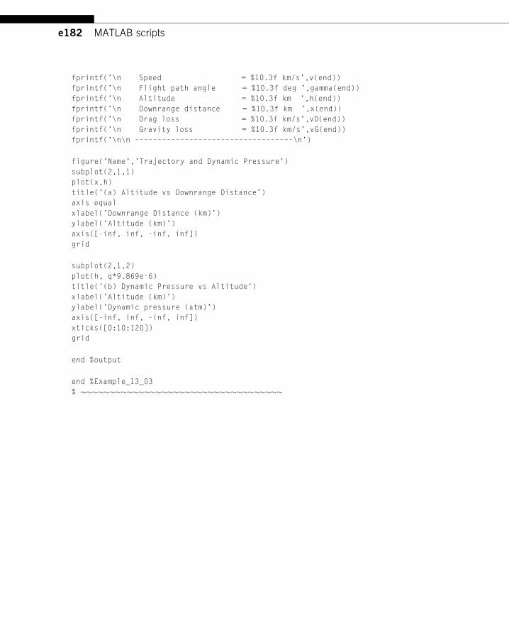
e182 MATLAB scripts
fprintf(’\n Speed = %10.3f km/s’,v(end))
fprintf(’\n Flight path angle = %10.3f deg ’,gamma(end))
fprintf(’\n Altitude = %10.3f km ’,h(end))
fprintf(’\n Downrange distance = %10.3f km ’,x(end))
fprintf(’\n Drag loss = %10.3f km/s’,vD(end))
fprintf(’\n Gravity loss = %10.3f km/s’,vG(end))
fprintf(’\n\n –––––––––––––––––––––––––––––––––––\n’)
figure(’Name’,’Trajectory and Dynamic Pressure’)
subplot(2,1,1)
plot(x,h)
title(’(a) Altitude vs Downrange Distance’)
axis equal
xlabel(’Downrange Distance (km)’)
ylabel(’Altitude (km)’)
axis([-inf, inf, -inf, inf])
grid
subplot(2,1,2)
plot(h, q*9.869e-6)
title(’(b) Dynamic Pressure vs Altitude’)
xlabel(’Altitude (km)’)
ylabel(’Dynamic pressure (atm)’)
axis([-inf, inf, -inf, inf])
xticks([0:10:120])
grid
end %output
end %Example_13_03
% �����������������������������������