Appendix A: Physical Constants and Functions For Use in Marine Meteorology

Appendix B:

Wind Force Scales

Appendix C: Unit Conversions

Edgar L Andreas

U.S. Army Cold Regions Research and Engineering Laboratory Hanover, New Hampshire 03755-1290

April 2005

2

LIST OF SYMBOLS B Beaufort number or force [see (B1.1)]

cp Specific heat of air at constant pressure

pc General value of the specific heat of air at constant pressure [see (A6.3)]

cpd Specific heat of dry air at constant pressure [see (A6.1)]

cpi Specific heat of pure ice at constant pressure [see (A6.10)]

cps Specific heat of seawater at constant pressure [see (A6.8)]

cpv Specific heat of water vapor at constant pressure [see (A6.2)]

cpw Specific heat of pure water at constant pressure [see (A6.9)]

D Thermal diffusivity of air [see (A11.2)]

D ' Thermal diffusivity of air modified for the effects of surface curvature [see (A13.2)]

da (= 103.7 10 m−× ) Effective diameter of an air molecule

Dg Diffusivity of an arbitrary gas in air [see (A12.4) and (A12.5)]

DgT Diffusivity of an arbitrary gas in air at a specified temperature and at pressure P0 [see Table A5]

Dg0 Diffusivity of an arbitrary gas in air at temperature T0 and pressure P0 [see Table A5]

dw (= 101.65 10 m−× ) Diameter of a water molecule

Dv Molecular diffusivity of water vapor in air [see (A12.1)]

vD ' Molecular diffusivity of water vapor in air modified for the effects of surface curvature [see (A13.3)]

e Water vapor pressure

esat Saturation pressure of water vapor [see (A4.1)–(A4.4)]

f (= RH/100) Fractional relative humidity

F Fujita number [see (B3.1)]

g Acceleration of gravity

Hs Sensible heat flux [see (A6.3)]

H1/3 Significant wave height [see Table B1]

k (= 23 11.38065 10 J K− −× ) Boltzmann constant

ka Thermal conductivity of air [see (A11.1)]

ak ' Thermal conductivity of air modified for the effects of surface curvature [see (A13.1)]

Lf Latent heat of fusion of water [see (A7.2)]

Ls Latent heat of sublimation of ice [see (A7.3)]

3

Lv Latent heat of vaporization of water [see (A7.1)]

Ma (= 3 128.9644 10 kg mol− −× ) Molecular weight of air

ms Mass of salt in a seawater sample

mw Mass of pure water in a seawater sample

Mw (= 3 118.015 10 kg mol− −× ) Molecular weight of water

P Barometric pressure

Pref Pressure measured a height zref above the sea surface [see (A14.4)]

Ps Barometric pressure at the sea surface [see (A14.4)]

P0 (= 1013.25 mb) Standard pressure; i.e., one atmosphere

Pr Molecular Prandtl number [see (A12.2)]

Q Specific humidity [see (A4.6)]

Qsat Saturation specific humidity [see (A4.7)]

r Mixing ratio [see (A4.9)]

R (= 1 18.31447 J mol K− − ) Universal gas constant

rsat Saturation mixing ratio [see (A4.10)]

r0 Radius of an atmospheric aerosol

RH Relative humidity in percent [see (A4.12) and (A4.15)]

s (= S/1000) Fractional salinity [see (A8.3)]

S Salinity in practical salinity units (psu)

Sc Molecular Schmidt number [see (A12.3)]

t Turbulent fluctuation in temperature [see (A6.3)]

T Temperature

Ta Air temperature

TC Temperature on the Celsius scale

Td Dew-point or frost-point temperature

Tf Freezing point of seawater [see (A5.3)]

TF Temperature on the Fahrenheit scale

TK Temperature on the Kelvin scale

Tv Virtual temperature [see (A3.8)]

vT Average virtual temperature [see (A14.4)]

Tvref Virtual temperature at some reference height

Tvs Virtual sea surface temperature

4

Twet Wet-bulb temperature

T0 (= 273.15 K) Standard temperature

U Surface-level wind speed [see (B3.1)]

U10 Wind speed at a height of 10 m [see (B1.1)]

w Turbulent fluctuation in vertical velocity [see (A6.3)]

z Height

zref A reference height [see (A14.4)]

αc (= 0.036) Empirical constant in the equation for the modified water vapor diffusivity [see (A13.3)]

αT (= 0.7) Empirical constant in the equation for the modified thermal conductivity [see (A13.1)]

∆T (= 72.16 10 m−× ) Empirical length scale in the equation for the modified thermal conductivity [see (A13.1)]

∆v (= 88.7 10 m−× ) Empirical length scale related to the mean free path of an air molecule and used in the equation for the modified water vapor diffusivity [see (A13.3)]

ηa Dynamic viscosity of air [see (A10.1)]

ηw Dynamic viscosity of pure water [see (A10.4)]

λa Mean free path of air molecules [see (A9.4)]

λv Mean free path of water vapor molecules in air [see (A9.5)]

νa Kinematic viscosity of air [see (A10.3)]

νsw Kinematic viscosity of seawater [see (A10.6)]

νw Kinematic viscosity of pure water [see (A10.5)]

ρa Density of moist air [see (A3.5) and (A3.7)]

aρ Air density in general [see (A6.3)]

ρd Density of dry air [see (A2.2) and (A3.2)]

ρd0 (= 31.2922kg m− ) Density of dry air at standard temperature and pressure [see (A2.2)]

ρsw Density of seawater [see (A5.2)]

ρv Density of water vapor (or absolute humidity) [see (A3.1)]

ρv,sat Saturation water vapor density

ρw Density of pure water [see (A5.1) and (A5.5)]

σsw Surface tension of an interface between water vapor and seawater [see (A8.5)]

5

σw Surface tension of an interface between water vapor and pure water [see (A8.1) and (A8.2)]

6

Appendix A: Physical Constants and Functions for Use in Marine Meteorology

A1. INTRODUCTION Studies of geophysical boundary layers always require kinematic and thermodynamic constants for the fluids involved. The most obvious examples are for the fluid densities: air, pure water, seawater, and water vapor. Boundary-layer studies frequently involve exchanging properties across interfaces; consequently, molecular properties like the kinematic viscosity, thermal conductivity, water vapor diffusivity, and surface tension are also necessary. In turn, the ratios of the molecular transport quantities—the Prandtl and Schmidt numbers—are recurring variables. Here, we summarize the values and functions for these and other quantities that are useful in marine meteorology. This summary is admittedly not all-encompassing. For example, we tend to focus on the quantities and the range of conditions for studies of air–land, air–sea, and air–sea–ice interaction. We also describe some microphysical quantities used in studies of aqueous solution droplets, like cloud droplets and sea spray. We tend to simply describe ways to calculate the quantities of interest without also explaining why you might want this quantity. Therefore, check any good book on atmospheric thermodynamics, such as Iribarne and Godson (1981), Pruppacher and Klett (1997), or Bohren and Albrecht (1998), for academic discussions of the thermodynamic quantities. A2. AIR DENSITY

Dry air obeys the ideal gas law,

ad

M PR T

ρ = , (A2.1)

where ρd is the density of dry air; Ma, the molecular weight of air; P, the barometric pressure; R, the universal gas constant; and T, the air temperature in kelvins. At standard temperature (T = T0 = 273.15 K) and pressure (P = P0 = 1013.25 mb), (A2.1) gives ρd0 = 1.2922 kg m–3. Therefore, (A2.1) also gives

0 0d d0

0 0

T TP P1.2922T P T P

⎛ ⎞ ⎛ ⎞⎛ ⎞ ⎛ ⎞ρ = ρ =⎜ ⎟ ⎜ ⎟⎜ ⎟ ⎜ ⎟⎝ ⎠ ⎝ ⎠⎝ ⎠ ⎝ ⎠

, (A2.2)

where ρd is in kg m–3 when P is in millibars and T is in kelvins. A3. WATER VAPOR DENSITY

Water vapor in the atmosphere also obeys the ideal gas law;

7

wv

M eR T

ρ = , (A3.1)

where ρv is the water vapor density, Mw is the molecular weight of water, and e is the partial pressure of the water vapor. To be rigorous, we need to recognize that, in (A2.1), the partial pressure of dry air is not the barometric pressure P but rather is approximately P – e. That is, in rigorous usage, (A2.1) should be

( )ad

M P eR T

−ρ = . (A3.2)

By rearranging (A3.1) and (A3.2), we can write the following expression for the barometric pressure:

( ) d v

a w

R T R TP P e eM Mρ ρ

= − + = + , (A3.3)

or

a a v

a w a

R T MP 1 1M M

⎡ ⎤⎛ ⎞ρ ρ= + −⎢ ⎥⎜ ⎟ ρ⎝ ⎠⎣ ⎦

. (A3.4)

Here, a d vρ = ρ + ρ (A3.5) is the density of moist air; and we recognize ρv/ρa as the specific humidity, Q (more on this soon). Equation (A3.4) rearranges to

( )

aa

M PR T 1 0.608Q

ρ =+

, (A3.6)

where a wM / M 1 0.608− = . Equation (A3.6) implies that (A2.1) is inaccurate by the factor (1 + 0.608Q) if we want the total air density. Since for normal atmospheric conditions Q is seldom larger than 0.035 kg kg–1, the term in parentheses in (A3.6) is always between 1.000 and 1.022. Therefore, (A2.1) may be accurate enough for many purposes. Nevertheless, we often rewrite (A3.6) as (e.g., Lumley and Panofsky 1964, p. 214)

aa

v

M PR T

ρ = (A3.7)

8

to preserve the form of (A2.1) while retaining the accuracy of (A3.6) by defining the virtual temperature ( )vT T 1 0.608Q= + . (A3.8) In effect, Tv is the temperature that dry air must have to produce the same density as moist air at the given barometric pressure. A4. WATER VAPOR VARIABLES Many types of instruments are available for measuring atmospheric water vapor. Some actually measure the water vapor density (the absolute humidity), but many measure derivative quantities such as the mixing ratio, the dew-point temperature, or the wet-bulb temperature. Hence, analyses and data reporting often require converting among the different water vapor variables. Schwerdtfeger (1976) and Pruppacher and Klett (1997, p. 106f.), among many others, give good summaries of water vapor variables.

A4.1. Vapor Pressure

If there is a fundamental water vapor quantity, it is the vapor pressure e. And for computational purposes, the saturation vapor pressure esat is usually the fundamental variable. We use Buck’s (1981) three equations for the saturation vapor pressure (cf. Brock and Richardson 2001, p. 86ff.). For vapor in saturation with a planar surface of pure water at temperature T between –20° and 50°C, Buck gives

( ) ( )6sat

17.502Te T 6.1121 1.0007 3.46 10 P exp240.97 T

− ⎛ ⎞= + × ⎜ ⎟+⎝ ⎠

, (A4.1)

where esat is in millibars when P, the barometric pressure, is also in millibars. For saturation over water at much lower temperatures, 40 T 0 C− °≤ ≤ ° , Buck (1981) gives

( ) ( )6sat

17.966Te T 6.1121 1.0007 3.46 10 P exp247.15 T

− ⎛ ⎞= + × ⎜ ⎟+⎝ ⎠

. (A4.2)

Use this relation, for example, to compute the saturation vapor pressure in clouds composed of deeply supercooled water droplets. Finally, if the vapor is in equilibrium with a surface of pure ice (or snow, for instance), Buck (1981) recommends the following equation for 50 T 0 C− °≤ ≤ ° :

( ) ( )6sat

22.452Te T 6.1115 1.0003 4.18 10 P exp272.55 T

− ⎛ ⎞= + × ⎜ ⎟+⎝ ⎠

. (A4.3)

9

As an alternative for the saturation vapor pressure over ice, Murphy and Koop (2005) give a more complex expression that extends over a wider temperature range,

165.15 T 0 C− °≤ ≤ ° ;

( ) ( )

( )

5 5 2sate T 0.01 1 10 P 4.923 0.0325T 5.84 10 T

5723.265exp 9.550426 3.53068ln T 0.00728332TT

− −⎡ ⎤= + − + ×⎣ ⎦⎡ ⎤• − + −⎢ ⎥⎣ ⎦

. (A4.4)

This gives esat in millibars for P in millibars and T in kelvins. Equations (A4.3) and (A4.4) differ insignificantly over their common range. We therefore prefer (A4.3) because it is mathematically simpler. Use (A4.4), however, for temperatures below –50°C. Figure A1 shows esat as a function of temperature for saturation over water, over supercooled water, and over ice. Instruments that measure the dew-point or frost-point temperature essentially provide the temperature T in (A4.1)–(A4.4). Hence, Figure A1 is equivalently a plot of saturation vapor pressure versus dew-point or frost-point temperature, depending on whether the surface in equilibrium is water or ice. When the water surface is not pure but, for example, is seawater with salinity S, the saturation vapor pressure is depressed to esat(T,S), where (e.g., Roll 1965, p. 262; List 1984, p. 373)

( )( )

sat

sat

e T,S1 0.000537S

e T= − . (A4.5)

Here, the salinity is in psu. Equation (A4.5) means that, for a typical open-ocean salinity of 35 psu, water vapor in saturation with the surface has a vapor pressure that is 98.1% of the vapor pressure over a pure water surface with the same temperature. The discussion naturally turns now to how to treat a sea ice surface. The point is often moot, however, because sea ice is usually snow covered, so we would just compute the saturation vapor pressure as that for pure ice using (A4.3) or (A4.4). If the surface is truly bare sea ice, on the other hand, such as for new ice in a freezing lead or summer sea ice when the snow has all melted, we could still reasonably just use the saturation vapor pressure relation for pure ice. Freezing seawater rejects salt; consequently, sea ice rarely has a surface salinity above 8 psu. If we assume that (A4.5) is also appropriate for sea ice—a reasonable assumption—the depression in vapor pressure over sea ice with salinity 8 psu would be only about 0.4%. Most humidity sensors cannot resolve such small changes in vapor pressure. Nevertheless, if such differences are important, (A4.5) should be adequate for quantifying them.

A4.2. Specific Humidity

Most other water vapor variables are calculated from the actual vapor pressure e and the saturation vapor pressure esat. For example, (A3.1) shows how to compute the water vapor density ρv from the vapor pressure. The saturation vapor density ρv,sat likewise comes from (A3.1) with esat substituted for e. The specific humidity is defined as

10

v

d v

Q ρ=

ρ + ρ , (A4.6)

and the saturation specific humidity is

v,satsat

d v,sat

Qρ

=ρ + ρ

. (A4.7)

Notice that, from (A3.1) and (A3.2),

( )

( )( )

w

w a

a w w

a

M e0.622 e / PM e M PQ

M P e M e 1 0.378 e / PM e1 1M P

= = =− + −⎛ ⎞

− −⎜ ⎟⎝ ⎠

. (A4.8)

That is, the specific humidity also derives from the vapor pressure. In SI units, specific humidity is given in kg kg–1.

A4.3. Mixing Ratio The mixing ratio is defined as

v

d

r ρ=

ρ , (A4.9)

and the saturation mixing ratio is

v,satsat

d

rρ

=ρ

. (A4.10)

As with (A4.8), we can also write r in terms of the vapor pressure. From (A3.1) and (A3.2),

( )

( )( )

w

w a

a

M e0.622 e / PM e M Pr eM P e 1 e / P1

P

= = =− −−

. (A4.11)

A4.4. Relative Humidity

Officially, the relative humidity (in percent) is defined as the ratio of mixing ratios (Bohren and Albrecht 1998, p. 198; Glickman 2000, p. 642f.),

11

sat

rRH 100r

⎛ ⎞= ⎜ ⎟

⎝ ⎠ . (A4.12)

From the definitions of mixing ratios, though, we see that

sat

sat

P eeRH 100P e e

⎛ ⎞⎛ ⎞ −= ⎜ ⎟⎜ ⎟−⎝ ⎠⎝ ⎠

. (A4.13)

We can rearrange this as

( )( )

sat sat sat2

sat sat

1 e / P e e e ee eRH 100 100 1e 1 e / P e P P

⎡ ⎤−⎛ ⎞ ⎛ ⎞ ⎡ − ⎤⎛ ⎞= − −⎢ ⎥⎜ ⎟ ⎜ ⎟ ⎜ ⎟⎢ ⎥− ⎝ ⎠⎣ ⎦⎝ ⎠ ⎝ ⎠⎣ ⎦ . (A4.14)

Over marine surface, for example, esat/P and e/P are usually less than 0.03, and e is rarely less than 0.5 esat. Hence, for practical purposes, we can generally ignore the term in square brackets in (A4.14); (A4.12) is, thus, equivalent to the traditional definition of relative humidity,

sat

eRH 100e

⎛ ⎞= ⎜ ⎟

⎝ ⎠ . (A4.15)

Furthermore, Bohren and Albrecht (1998, p. 186) prefer (A4.15) to (A4.12) because it better reflects the physics of evaporation and condensation processes. We likewise use (A4.15) as our definition of relative humidity. Table A1 shows the relative humidity as a function of air temperature and dew-point temperature, where we use (A4.15) to define relative humidity.

A4.5. Wet-Bulb Temperature

The wet-bulb temperature, Twet, is another common humidity variable (e.g., Schwerdtfeger 1976, p 50ff.). A wetted thermometer will read lower than the ambient air temperature because of evaporation (but higher with condensation), and that rate of evaporation depends on the mixing ratio. At equilibrium, a well-ventilated wet-bulb thermometer obeys (Andreas 1995; Bohren and Albrecht 1998, p. 218ff) ( )( ) ( ) ( )p a a wet v a sat wetc T T T L T r T r− = −⎡ ⎤⎣ ⎦ , (A4.16) where cp is the specific heat of dry air at temperature Ta, Lv is the latent heat of vaporization at Ta, r is the ambient mixing ratio, and rsat is the saturation mixing ratio at the wet-bulb temperature. Rearranging (A4.16) shows that the wet-bulb temperature predicts the mixing ratio,

( ) ( )( ) ( )p a

sat wet a wetv a

c Tr r T T T

L T= − − . (A4.17)

12

And in light of (A4.11),

( ) ( ) ( )( ) ( )p aa

sat wet a wetsat w v a

P e c TMP ee e T T TP e M L T

−⎛ ⎞−= − −⎜ ⎟−⎝ ⎠

, (A4.18)

which is approximately

( ) ( )( ) ( )p a

sat wet a wetv a

P c Te e T T T

0.622 L T− − . (A4.19)

That is, the wet-bulb temperature also predicts the vapor pressure. Table A2 shows the vapor pressure computed from (A4.19) for a range of Ta and a wetT T− values. Equations (A4.16)–(A4.19) apply to perfect wet-bulb thermometers. Schwerdtfeger (1976, p. 51f.) and Brock and Richardson (2001, p. 94) describe some second-order corrections that may be necessary to account for ventilation rate, radiative effects, and the size of the wet bulb. A5. WATER DENSITY

The literature contains several modern expressions for the density of pure water, ρw. Any one would probably be accurate enough for the purposes of this handbook. This one is Gill’s (1982, p. 599):

2 3 2

w

4 3 6 4 9 5

999.842594 6.793952 10 T 9.095290 10 T

1.001685 10 T 1.120083 10 T 6.536332 10 T

− −

− − −

ρ = + × − ×

+ × − × + × . (A5.1)

It gives ρw in kg m–3 for a barometric pressure of one atmosphere when T is between 0° and 40°C. To find the density of seawater, ρsw, with temperature T and salinity S for pressures near one atmosphere, Gill (1982, p. 599) gives

3 5 2sw w

7 3 9 4

3/ 2 3 4 6 2

4 2

S(0.824439 4.0899 10 T 7.6438 10 T

8.2467 10 T 5.3875 10 T )

S ( 5.72466 10 1.0227 10 T 1.6546 10 T )

4.8314 10 S

− −

− −

− − −

−

ρ = ρ + − × + ×

− × + ×

+ − × + × − ×

+ ×

. (A5.2)

This is appropriate for S in [0, 42 psu] and T in [Tf, 40°C], where Tf is the freezing point of seawater with salinity greater than 0 psu.

13

Gill (1982, p. 602) give Tf as a function of salinity for S between 0 and 40 psu; but we prefer Kester’s (1974) formula, which is always within 0.01°C of Gill’s for S in [1, 40 psu], because it is easier to invert. Kester gives Tf in °C as 2 5 2

fT 0.0137 5.1990 10 S 7.225 10 S− −= − − × − × . (A5.3) In turn, if we know that the seawater is at its freezing point, we can invert (A5.3) to find the corresponding salinity, ( ) 1/ 22 3 3 4

fS 3.598 10 6.920 10 2.7030 10 2.890 10 T 0.0137− −⎡ ⎤= − × + × × − × +⎣ ⎦ . (A5.4) For supercooled pure water in the temperature interval [ ]33 ,0 C− ° ° , Pruppacher and Klett (1997, p. 87) give

2 3 2 4 3

w

6 4 7 5 9 6

999.86 6.690 10 T 8.486 10 T 1.518 10 T

6.9984 10 T 3.6449 10 T 7.497 10 T

− − −

− − −

ρ = + × − × + ×

− × − × − × . (A5.5)

Here, again, ρw is in kg m–3 when T is in °C. Pruppacher and Klett have taken (A5.5) directly from Hare and Sorensen (1987). For completeness, we also include in this section an equation for the density of pure ice, ρi. Pruppacher and Klett (1997, p. 79f.) give 4 2

i 916.7 0.175T 5.0 10 T−ρ = − − × , (A5.6) which yields ρi in kg m–3 for T in °C. Pruppacher and Klett claim that this relation fits the experimental data for T in [ ]180 ,0 C− ° ° . On comparing the predictions of (A5.6) with Hobbs’s (1974, p. 348) tabulation of ρi, we can further say that (A5.6) is accurate to better than 0.5% over this range. A6. SPECIFIC HEAT

A6.1. Specific Heat of Dry Air

The specific heat of air appears recurrently in studies of the atmospheric boundary layer. Using data from Hilsenrath et al. (1960), we have obtained the following polynomial prediction for the specific heat of dry air at constant pressure: 2

pdc 1005.60 0.017211T 0.000392T= + + . (A6.1) This gives cpd in J kg–1 °C–1 for temperature T between –40° and 40°C and for barometric pressures near one atmosphere. Equation (A6.1) has a minimum of 1 11005.41J kg C− −° at

21.95°C− .

14

A6.2. Specific Heat of Water Vapor

Reid et al. (1987, p. 656f., 668) give a polynomial expression for the specific heat of water vapor at constant pressure for barometric pressures near one atmosphere. The temperature in their polynomial is in kelvins, however, and their units of cpv are J mol–1 °C–1. We have therefore converted their polynomial to 1 4 2 7 3

pvc 1858 3.820 10 T 4.220 10 T 1.996 10 T− − −= + × + × − × , (A6.2) which give cpv in J kg–1 °C–1 when T is in °C. Equation (A6.2) should be accurate for all near-surface atmospheric temperatures.

A6.3. In the Turbulent Sensible Heat Flux

A frequent use for the specific heat of air is in finding the turbulent sensible heat flux, which is defined as pasH c wt= ρ . (A6.3) Here, w is the turbulent fluctuation in vertical wind velocity, t is the turbulent fluctuation in air temperature, and the overbar denotes a time average. The tildes over the ρa and the cp terms in (A6.3) denote these as general values of the air density and specific heat of air at constant pressure because confusion exists as to which values constitute the proper definition of sensible heat flux. Most of the boundary-layer community simply use ρa, the density of moist air, for aρ and

cpd for pc . Businger’s (1982) analysis confirms that this is proper practice for micrometeorological studies. That is, (A6.3) would be s a pdH c wt= ρ . (A6.4) On the other hand, when long time intervals or global averages define the scope of the study—for example, in balancing the hydrological cycle—Businger (1982) explains that the reference temperature for enthalpy transfer must be chosen carefully. When such “careful bookkeeping of the energy” is necessary, Businger concludes that the sensible heat flux must be expressed as ( )s d pd v pvH c c wt= ρ + ρ . (A6.5) Fuehrer and Friehe’s [2002, Eq. (114)] extensive thermodynamic analysis yields essentially this same result, although they give it as general result—not one necessary only for large areal averages. They also include two other small terms in (A6.5) that are associated with the flux of water vapor between temperature reference states. As a practical exercise, we can check how different (A6.4) and (A6.5) are. We can convert (A6.5) into a form similar to (A6.4),

15

pv pds a pd

pd

c cH c 1 Q wt

c

⎡ ⎤⎛ ⎞−= ρ +⎢ ⎥⎜ ⎟⎜ ⎟⎢ ⎥⎝ ⎠⎣ ⎦

. (A6.6)

Using (A6.1) and (A6.2), we see that ( )pv pd pdc c / c− ranges from 0.861 to 0.833 for air temperatures between –40° and 40°C. Hence, we approximate (A6.6) as (cf. Larsen and Busch 1974) ( )s a pdH c 1 0.85Q wtρ + . (A6.7) As we mentioned earlier, Q is seldom larger than 0.035 kg kg–1 in the natural atmosphere; and it would attain this value, probably, only over the tropical ocean. Hence, (A6.5) yields values of the sensible heat flux that are, at most, 3% larger than the values from (A6.4). In many applications, this is a negligible difference since wt usually is measured to no better than ±10%. And at temperatures below 0°C, where Q is less than 0.004 kg kg–1, (A6.4) and (A6.5) differ by much less than 1%.

A6.4. Specific Heat of Water Both temperature and salinity influence the specific heat of seawater at constant pressure, cps. Neumann and Pierson (1966, p. 47) tabulate values of cps that come from data collected by Cox and Smith (1959). Horne (1969, p. 68) gives a functional expression for cps in terms of temperature and salinity that he converted from a similar expression that Bromley et al. (1967) deduced from their own measurements. Millero et al. (1973) also reported measurements of cps and fitted an equation to these measurements in terms of temperature and chlorinity. Gill (1982, p. 601) converted this to an expression in terms of temperature and salinity. The following is essentially Gill’s equation, although we have modified it slightly to better represent the precision that Millero et al. implied in their fitting coefficients:

( )

( )

3 2ps pw

3/ 2 3 5 2

c c S 7.6444 0.10728T 1.384 10 T

S 0.177 4.08 10 T 5.35 10 T

−

− −

= + − + − ×

+ − × + × . (A6.8)

Here, cpw is the specific heat of pure water, 2 3 3 5 4

pwc 4217.4 3.720283T 0.1412855T 2.654387 10 T 2.093236 10 T− −= − + − × + × . (A6.9) In (A6.8) and (A6.9), T is in °C and ranges from Tf to 40°C; in (A6.8), S is in psu and ranges from 0 to 40 psu. The pressure is assumed to be one atmosphere. Table A3 shows values of cps that result from (A6.8). The values in Table A3 are quite compatible with the values in Neumann and Pierson’s (1966, p. 47) table, which are based on Cox and Smith’s (1959) data. The values in Table A3,

16

however, have some systematic differences from the results from Bromley et al. (1967; also Horne 1969, p. 67f.), especially for fresh water in the lower part of the temperature range. For example, Bromley et al. report 1 1

pwc 4207 J kg C− −= ° for T = 0°C, while Table A3 gives 1 14217 J kg C− −° . Therefore, we conclude that (A6.8) and (A6.9) are accurate to roughly

1 13J kg C− −± ° (cf. Bromley et al. 1967; Millero et al. 1973).

A6.5. Specific Heat of Ice Murphy and Koop (2005) give a new expression for the specific heat of ice for temperatures down to 20 K. Because their units, however, are J mol–1 K–1, we convert their expression to predict cpi in J kg–1 K–1 using 3 1

wM 18.015 10 kg mol− −= × . The result is ( )2

pic 114.19 8.1288T 3.421T exp T /125.1⎡ ⎤= − + + −⎣ ⎦ , (A6.10)

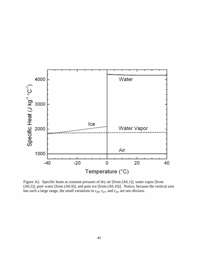
in which T must be in kelvins. Murphy and Koop use (A6.10), for example, to derive their expression for the saturation vapor pressure over ice, (A4.4) above. Figure A2 compares values for the specific heats of air, pure water, ice, and water vapor for temperatures between –40° and 40°C. A7. LATENT HEAT Fleagle and Businger (1980. p. 113) give the following equations for the latent heats associated with the phase transitions of water molecules: Latent heat of vaporization, ( ) 5

vL 25.00 0.02274T 10= − × ; (A7.1) Latent heat of fusion, 5

fL 3.34 10= × ; (A7.2) Latent heat of sublimation, ( ) 5

sL 28.34 0.00149T 10= − × . (A7.3) Each of these gives the latent heat in J kg–1 when the temperature T is in °C. The value for Lf in (A7.2) is appropriate only near 0°C because Lf decreases with decreasing temperatures. Hobbs’s (1974, p. 361) tabulation of Lf for temperatures below 0°C disagrees dramatically with a similar tabulation in the Smithsonian Meteorological Tables (List 1984, p. 343), however. The functions for Lv and Ls, on the other hand, agree quite well with the Smithsonian tabulation. The Lv values predicted by (A7.1) are within 0.3% of the Smithsonian values for temperatures from 0° to 60°C, and the Ls values from (A7.3) are within 0.2% of the Smithsonian values for temperatures between –50° and 0°C.

17

A8. SURFACE TENSION OF WATER Vargaftik et al. (1983) tabulate consensus values for the surface tension of pure water for temperatures between 0°C and the critical temperature, 374°C (Bohren and Albrecht 1998, p. 207ff.). They also develop from these data the following relation for computing the surface tension of pure water:

1.256

w374.00 T 374.00 T0.2358 1 0.625

647.15 647.15− ⎡ − ⎤⎛ ⎞ ⎛ ⎞σ = −⎜ ⎟ ⎜ ⎟⎢ ⎥⎝ ⎠ ⎝ ⎠⎣ ⎦

. (A8.1)

This gives σw in J m–2 when the water temperature T is in °C. This equation predicts exactly the values of surface tension that Lide (2001, p. 6-3) tabulates and matches the values in Batchelor (1970, p. 597) to within about 0.1%. For temperatures between –45° and 0°C, Pruppacher and Klett (1997, p. 130) suggest computing the surface tension of pure water from

2 4 5 2 6 3

w

7 4 9 5 11 6

7.593 10 1.15 10 T 6.818 10 T 6.511 10 T

2.933 10 T 6.283 10 T 5.285 10 T

− − − −

− − −

σ = × + × + × + ×

+ × + × + × , (A8.2)

which again gives σw in J m–2 for T in °C. Unfortunately, (A8.1) and (A8.2) do not meet at 0°C. Equation (A8.1) predicts 2 27.656 10 J m− −× there, while (A8.2) gives 2 27.593 10 J m− −× . The former value is probably the more accurate one. Pruppacher and Klett (1978, p. 107) likewise give an expression for the surface tension of an interface between water vapor and saline water. That expression, however, quantifies the salinity in terms of ms/mw, where mw is the mass of pure water per unit volume and ms is the mass of dissolved salt in the volume. Since the definition of salinity is

s

w s

msm m

=+

, (A8.3)

we see that

s

w

m sm 1 s

=−

, (A8.4)

where s is the fractional salinity [s = S(in psu)/1000]. Hence, we convert Pruppacher and Klett’s (1978) expression for the surface tension at a seawater interface to

2sw w

s2.77 101 s

− ⎛ ⎞σ = σ + × ⎜ ⎟−⎝ ⎠

, (A8.5)

18

where σw comes from (A8.1) or (A8.2), depending on the water temperature. The coefficient multiplying the salinity term in (A8.5) is virtually the same value that Hänel (1976) recommends. Equation (A8.5) should be accurate for temperatures in [ ]25 , 40 C− ° ° and S in [ ]0, 260 psu . A9. MEAN FREE PATHS OF AIR AND WATER VAPOR MOLECULES The mean free path of a gas molecule is an estimate of the distance it travels between collisions with other molecules in the gas. Starting with equations that Wagner [1982, Eqs. (A5.55), (A5.56)] gives, we derive these expressions for the mean free paths of air molecules (λa) and water vapor molecules (λv) in air:

( )a 2

a

k T2 P e d

λ =π −

, (A9.1)

( )( )v 2

a w

4k T1.622 P e d d

λ =π − +

. (A9.2)

In these, k is the Boltzmann constant; T, the kelvin temperature; P and e, the barometric pressure and the water vapor pressure in pascals; and da and dw, the diameters of air and water molecules. Equation (A9.1) is essentially the same as Reif’s (1967) expression for the mean free path of air molecules,

a 2a

k T2 P d

λ =π

. (A9.3)

In (A9.1) and (A9.2), λa and λv quantify the distance between consecutive collisions, not the distance between collisions between molecules of the same species. That is, a water vapor molecule will likely hit an air molecule next; λv estimates the distance from the previous to this next collision. Using values for da and dw of 103.7 10 m−× and 101.65 10 m−× , respectively (personal communication, James H. Cragin 2000), and expressing P and e in millibars, we simplify (A9.1) and (A9.2) to

7

a2.3 10 T

P e

−×λ =

− , (A9.4)

7

v4.8 10 T

P e

−×λ =

− . (A9.5)

In these, λa and λv are in meters when T is in kelvins and P and e are in millibars. For example, when T = 293K and P – e = 1000 mb,

19

8

a 6.7 10 m−λ = × , (A9.6) 7

v 1.4 10 m−λ = × . (A9.7) For comparison, Pruppacher and Klett (1978, p. 323) state without proof that 8

a 6.6 10 m−λ = × for P = P0 and T = 293.15 K. Bohren and Albrecht (1998, p. 68) estimate 7

a 10 m−λ = for pressures near one atmosphere. A10. MOLECULAR VISCOSITY

A10.1. Air

Hilsenrath et al. (1960, p. 10) give the following expression for the dynamic viscosity of air:

6 3/ 2

a1.458 10 T

T 110.4

−×η =

+ . (A10.1)

Here, ηa is in kg m–1 s–1 when T is in kelvins, and they suggest that this relation is accurate for a pressure of one atmosphere for temperatures between 100 and 1900 K. The kinematic viscosity of air, νa, however, occurs more commonly in boundary-layer studies. We can obtain this from ηa as

aa

d

ην ≡

ρ . (A10.2)

We have combined this definition, (A2.2), and (A10.1) to obtain a polynomial expression for predicting νa for the temperature range [ ]50 ,50 C− ° ° ; ( )5 3 6 2 9 3

a 1.326 10 1 6.542 10 T 8.301 10 T 4.840 10 T− − − −ν = × + × + × − × . (A10.3) Here, νa is in m2 s–1, and T is in °C. Figure A3 shows (A10.3) plotted as a function of temperature; Table A4 lists these values. The predictions from (A10.3) agree to three significant figures with values tabulated in Goldstein (1965, p. 7) and Batchelor (1970, p. 594).

A10.2. Water Reid et al. (1987, p. 441, 455) give the following expression for the dynamic viscosity of pure water: ( )3 3 1 2 5 2

w 10 exp 24.71 4.209 10 T 4.527 10 T 3.376 10 T− − − −η = − + × + × − × . (A10.4)

20

As with (A10.1), here ηw is in kg m–1 s–1, and the temperature is in kelvins. Because Neumann and Pierson (1966, p. 52) suggest that salinity and pressure affect the dynamic viscosity of water only slightly, we compute the kinematic viscosity of pure water (νw) and seawater (νsw) from

ww

w

ην =

ρ (A10.5)

and

wsw

sw

ην =

ρ . (A10.6)

In these, νw and νsw are in m2 s–1; and ρw and ρsw come from (A5.1) and (A5.2), respectively. As examples of these calculations, for T = 20°C, S = 34 psu, and pressures near one atmosphere, we find 3 1 1

w 1.018 10 kg m s− − −η = × , 3w 998.2kg m−ρ = , 3

sw 1024.0kg m−ρ = , 6 2 1

w 1.019 10 m s− −ν = × , and 6 2 1sw 0.994 10 m s− −ν = × . In particular, these ηw and νw values and

values we have calculated at other temperatures are within 3% of values tabulated in Horne (1969, p. 486) and Batchelor (1970, p. 597). A11. THERMAL CONDUCTIVITY AND THERMAL DIFFUSIVITY OF AIR Hilsenrath et al. (1960, p. 70) also tabulate the thermal conductivity of air, ka. We have fitted their data for temperatures between –193° and 277°C with the following polynomial: ( )2 3 6 2

ak 2.411 10 1 3.309 10 T 1.441 10 T− − −= × + × − × . (A11.1) This gives ka in W m–1 °C–1 for temperature T in °C. The thermal diffusivity D is analogous as a molecular transport variable to the kinematic viscosity νa. We define D as

a

d p

kDc

=ρ

, (A11.2)

which has units of m2 s–1. Figure A3 plots D as a function of temperature, while Table A4 lists values for normal atmospheric boundary layer temperatures. Notice that, in general, ρa and cp in (A11.2) should include the effects of atmospheric water vapor. We have ignored those small effects in creating Figure A3 and Table A4 because (A11.1) predicts the thermal conductivity of dry air. We presume that including water vapor effects in ka would tend to offset the effects of water vapor in ρa and cp and would, thus, yield a thermal conductivity D comparable to the dry-air value that we have calculated.

21

A12. MOLECULAR DIFFUSIVITIES OF GASES IN AIR

A12.1. Water Vapor Hall and Pruppacher (1976) developed the following expression for the molecular diffusivity of water vapor in air:

1.94

5 0v

0

PTD 2.11 10T P

− ⎛ ⎞ ⎛ ⎞= × ⎜ ⎟ ⎜ ⎟⎝ ⎠⎝ ⎠

. (A12.1)

This gives Dv in m2 s–1 for temperature T in kelvins and pressure P in millibars. Hall and Pruppacher explain that no good measurements of Dv exist for temperatures below 0°C. Therefore, they obtain (A12.1) by extrapolating measurements above freezing to subfreezing temperatures. Still, Hall and Pruppacher claim that (A12.1) applies over the temperature interval [ ]80 , 40 C− ° ° . Pruppacher and Klett (1978, p. 413) originally recommended (A12.1), and Pruppacher and Klett (1997, p. 503) still do. Figure A3 and Table A4 compare values of Dv with νa and D. The Prandtl (Pr) and Schmidt (Sc) numbers compare the relative efficiencies of molecular exchange processes. The molecular Prandtl number for air is

aPrDν

≡ , (A12.2)

and the molecular Schmidt number for air is

a

v

ScDν

≡ . (A12.3)

We can compute these from (A10.3), (A11.2), and (A12.1). Table A4 also lists values of Pr and Sc for P = 1000 mb and temperatures in the range [ ]40 , 40 C− ° ° .

A12.2. Other Atmospheric Gases The molecular diffusivities of atmospheric trace gases such as carbon dioxide, methane, and nitrous oxide also occur in atmospheric boundary layer research. Reid et al. (1987, p. 587) give a semi-empirical expression, which they adapted from Fuller et al. (1969), to predict how the diffusivities of these trace atmospheric gases depend on temperature and pressure. Table A5 lists diffusivities in air for several environmentally important gases. We have computed some of these (labeled “Dg0, Reid et al.”) for T0 = 273.15 K and P0 = 1013.25 mb from equation (11-4.4) and Table 11.1 in Reid et al. (1987). For comparison, we also include in Table A5 diffusivity values (labeled DgT) at temperatures of 0°C (273.15 K) or 25°C (298.15 K) that Thibodeaux (1979, 1996) tabulates. Thibodeaux, however, does not mention the barometric pressure corresponding to his values; we therefore assume it is approximately one atmosphere.

22

Equation (11-4.4) in Reid et al. (1987) implies a general expression for how the diffusivities of gases in air depend on temperature and pressure,

1.75

0g g0

0

PTD DT P

⎛ ⎞ ⎛ ⎞= ⎜ ⎟ ⎜ ⎟⎝ ⎠⎝ ⎠

. (A12.4)

In this, Dg is in m2 s–1, T is in kelvins, P is in millibars, and Dg0 is the value at T0 and P0 in Table A5. Alternatively, we could just as well substitute Thibodeaux’s (1979, 1996) values for DgT in place of Dg0 in (A12.4), replace T0 with the tabulated temperature, and assume that Thibodeaux’s listed values all correspond to pressure P0. Massman (1998) also reviews the diffusivities of various gases in air in the context of an equation like (A12.4) but assumes that the exponent is 1.81:

1.81

0g g0

0

PTD DT P

⎛ ⎞ ⎛ ⎞= ⎜ ⎟ ⎜ ⎟⎝ ⎠⎝ ⎠

. (A12.5)

Table A5 lists the values that he recommends for Dg0. Coincidently, the Smithsonian Meteorological Tables (List 1984, p. 395) also suggests a relation like (A12.5) for the diffusivities of gases in air. Comparing the DgT values reported at 273.15 K directly with the Dg0 values in Table A5 or using (A12.4) or (A12.5) to convert the Reid et al. (1987), Massman (1998), or Thibodeaux (1979, 1996) values to the same temperature lets us evaluate the uncertainty in these gas diffusivities. For example, the four diffusivities listed in Table A5 for carbon dioxide have a spread of only 5 2 10.06 10 m s− −× at 0°C. The diffusivities for ammonia, on the other hand, have a spread of about 5 2 10.5 10 m s− −× at 0°C. Table A5 also includes four new estimates of the water vapor diffusivity to compare with (A12.1). The two values from Thibodeaux (1979, 1996) both predict 5 2 1

vD 2.20 10 m s− −= × at 0°C. The comparable value that we predict from Reid et al. (1987) is 5 2 1

vD 2.15 10 m s− −= × , while Massman (1998) recommends 5 2 1

vD 2.18 10 m s− −= × . Hall and Pruppacher’s (1976) equation, (A12.1), gives 5 2 1

vD 2.11 10 m s− −= × at 0°C and 1013.25 mb. Consequently, we conclude that the diffusivities for the gases listed in Table A5 are typically known to an accuracy of ±3%. Massman similarly concludes that most of the diffusivities listed in Table A5 have an absolute uncertainty that is no more than 5–9%, though the tabulated diffusivities for O3, NO, and NO2 might be uncertain by 25% because of the paucity of data for these molecules. A13. EFFECTS OF SURFACE CURVATURE ON ka AND Dv The transfers of heat and moisture at the surface of small atmospheric particles, like cloud droplets, sea spray droplets, snowflakes, and aerosols, cannot strictly be parameterized in terms of the ka and Dv values given above. Because of the extreme curvature of the surface of these small particles, the air around them no longer behaves as a continuum. This is the so-called Kelvin effect (e.g., Pruppacher and Klett 1997, p. 170). Likewise, surface curvature will

23

also affect the transfers of heat and moisture around the snow grains in a snowpack, which is always porous. Pruppacher and Klett (1997) present equations to account for how these curvature effects modify ka and Dv (also Andreas 1989, 1990, 1995). For predicting the effects of curvature on ka, they give (Pruppacher and Klett 1997, p. 509)

aa 1/ 2

0 a a

0 T 0 T a p

kk 'r k 2 M

r r c R T

=⎛ ⎞π

+ ⎜ ⎟+ ∆ α ρ ⎝ ⎠

. (A13.1)

In this, ak ' (in W m–1 K–1) is the thermal conductivity modified for curvature effects, r0 is the particle radius in meters, ∆T ( 72.16 10 m−= × ) and αT (= 0.7) are empirical constants, and T is again the kelvin temperature. In (A13.1), we recognize ka/ρacp from (A11.2) as the thermal diffusivity D. Hence, if we divide (A13.1) by ρacp, we get an analogous expression for curvature effects on the thermal diffusivity,

1/ 2

0 a

0 T 0 T

DD 'r 2 MD

r r R T

=⎛ ⎞π

+ ⎜ ⎟+ ∆ α ⎝ ⎠

. (A13.2)

This predicts the modified thermal diffusivity in m2 s–1. Similarly, Pruppacher and Klett (1997, p. 506) give the following equation for predicting how surface curvature influences the vapor diffusivity around small particles:

vv 1/ 2

0 v w

0 v 0 c

DD 'r D 2 M

r r R T

=⎛ ⎞π

+ ⎜ ⎟+ ∆ α ⎝ ⎠

. (A13.3)

Here, vD ' (in m2 s–1) is the water vapor diffusivity modified for curvature effects, and αc (= 0.036) and ∆v ( 8

a1.3 8.7 10 m−= λ = × for typical sea-level temperature and pressure) are empirical constants. Figure A4 compares ak ' with ka and vD ' with Dv for particles with radii between 0.1 and 1000 µm, which is a typical size range for sea spray droplets (cf. Andreas 1989). According to this figure, curvature effects significantly influence sensible heat transfer only around particles with radii less than about 5 µm. In contrast, surface curvature significantly decreases the rate of vapor diffusion around particles with radii up to about 200 µm.

24

A14. BAROMETER CORRECTION Computing the turbulent surface fluxes—for example, the sensible heat flux through (A6.7)—requires the air density right at the air-sea interface. Though this density can be calculated from (A3.7), using this equation requires the virtual surface temperature (Tvs) and the barometric pressure right at the air-sea interface (Ps). The barometer, however, is rarely at sea level but may be on the bridge, for instance, several tens of meters above the sea surface. Because, near the surface, pressure typically falls at about 10.12mbm− as height increases, we derive a correction here to adjust the pressure read at reference height zref (Pref) to sea level pressure. The hydrostatic equation,

a

1 P gz∂

= −ρ ∂

, (A14.1)

is the basis for this correction. Here z is the height, and g is the acceleration of gravity. Substituting the ideal gas law, (A3.7), into (A14.1) gives

a

v

1 P g MP z R T∂

= −∂

. (A14.2)

Integrating this equation from the reference height down to the surface (at z = 0) yields

P 0s a

P zref ref v

dP g M dzP R T

= −∫ ∫ . (A14.3)

The left side here integrates easily. On the right side, Tv is the only variable that depends on z; but that dependence is fairly weak within a few tens of meters of the sea surface. Therefore, we can assume Tv is essentially constant in (A14.3) and pull it out of the integral. Possible values to use for this constant ( vT ) are Tvs or ( )vs vref0.5 T T+ , where Tvref is the virtual temperature at some reference height above the surface. With this simplification, (A14.3) becomes

a refs ref

v

g M zP P expR T

⎛ ⎞= ⎜ ⎟

⎝ ⎠ . (A14.4)

Thus, for example, if refP 1000.0mb= , 2g 9.81ms−= , vT 290K= , and refz 30m= , then

sP 1003.5mb= .

25

Appendix B: Wind Force Scales

B1. BEAUFORT SCALE

A common way to describe wind and sea state is with the Beaufort Scale. In the early nineteenth century, Admiral Sir Francis Beaufort developed a wind scale based on the behavior of sailing ships (Huler 2004). In 1838, the British Admiralty adopted this scale as a method for unifying the reporting of winds at sea. But not until the early twentieth century did that scale emerge as the descriptive list of wind effects on both land and seat that we now know as the Beaufort Scale (Huler 2004). In effect, the Beaufort number or force B is related to the wind speed (in m s–1) at a standard reference height of 10 m, U10, through (List 1984, p. 119; Strangeways 2001) 3/ 2

10U 0.836B= . (B1.1) But the key feature of the Beaufort Scale is that it associates U10 and B with a description of wind, sea state, and wind effects on land and, thus, provides an estimate of U10 from visual observations alone (e.g., Bowditch 1977, p. 1059; List 1984, p. 119). Table B1 shows the Beaufort Scale and includes descriptions of conditions for a given Beaufort force over both land and sea. B2. SAFFIR-SIMPSON SCALE The Beaufort Scale classifies all ocean storms with surface-level winds above 32.7 m s–1 as hurricanes. But conditions at sea and when the storm comes ashore vary widely depending on the wind speed. The Saffir-Simpson Scale, developed by Herbert Saffir and Bob Simpson, further divides hurricanes into five categories. Table B2 shows the Saffir-Simpson Scale. At sea, storms are assigned to a Saffir-Simpson category on the basis of their maximum surface-level wind speed and minimum central pressure. Storms may change category during their lifetime as they intensify or degrade. The “Storm Surge” listed in Table B2 is the height of the ocean wave that comes ashore ahead of the storm. The values shown give a typical range; the actual storm surge will depend on the slope of the continental shelf. The main relevance of the Saffir-Simpson Scale is that it attempts to forecast flooding and damage if the storm does move onshore. The “Effects” column in the table lists these predictions. Effects range from minor for a Category 1 storm to catastrophic, as they were with Mitch, a 1998 Category 5 hurricane that killed over 800 people in Honduras and Nicaragua. B3. FUJITA SCALE

Similarly, the Fujita Scale categorizes tornadoes in terms of their maximum wind speed and the damage they cause (Fujita 1981; Glickman 2000, p. 322f.). Table B3 shows the Fujita Scale. Fujita (1981) associated the lower surface-level wind speed limit for a tornado category with the Fujita number F through the expression

26

( )3/ 2U 6.30 F 2= + , (B3.1) where U is the wind speed in m s–1.

27

Appendix C: Unit Conversions

C1. TEMPERATURE The three temperature scales in common use in meteorology are the Celsius (°C) scale, the Fahrenheit (°F) scale, and the Kelvin (K) scale. The temperature of absolute zero is 0 K or

273.15 C− ° ; hence, the Celsius temperature (TC) is related to the Kelvin temperature (TK) by C KT T 273.15= − . (C1.1) That is, a temperature step of 1°C is equivalent to a temperature step of 1 K. Likewise, the following equations relate temperatures on the Fahrenheit (TF) and Celsius scales: ( )F CT 9 / 5 T 32= + , (C1.2) and ( )( )C FT 5/ 9 T 32= − . (C1.3) Here are a few examples of using these equations to find comparable Fahrenheit and Celsius temperatures: 40 F 40 C− ° =− ° , 32 F 0 C° = ° , 68 F 20 C° = ° , and 212 F 100 C° = ° . C2. OTHER UNITS Table C1 lists conversions among Système International (SI) units and other non-SI units that occur in marine meteorology.

28

REFERENCES

Andreas, E. L, 1989: Thermal and size evolution of sea spray droplets. CRREL Rep. 89-11, U. S. Army Cold Regions Research and Engineering Laboratory, 37 pp. (NTIS: AD A210484.)

, 1990: Time constants for the evolution of sea spray droplets. Tellus, 42B, 481–497.

, 1995: The temperature of evaporating sea spray droplets. J. Atmos. Sci., 52, 852–862.

Batchelor, G. K., 1970: An Introduction to Fluid Dynamics. Cambridge University Press, 615 pp.

Bohren, C. F., and B. A. Albrecht, 1998: Atmospheric Thermodynamics. Oxford University Press, 402 pp.

Bowditch, N., 1977: American Practical Navigator. Vol. 1. Publication No. 9, Defense Mapping Agency Hydrographic Center, Washington, D.C., 1386 pp.

Brock, F. V., and S. J. Richardson, 2001: Meteorological Measurement Systems. Oxford University Press, 290 pp.

Bromley, L. A., V. A. Desaussure, J. C. Clipp, and J. S. Wright, 1967: Heat capacities of sea water solutions at salinities of 1 to 12% and temperatures of 2° to 80°C. J. Chem. Engng. Data, 12, 202–206.

Buck, A. L., 1981: New equations for computing vapor pressure and enhancement factor. J. Appl. Meteor., 20, 1527–1532.

Businger, J. A., 1982: The fluxes of specific enthalpy, sensible heat and latent heat near the Earth’s surface. J. Atmos. Sci., 39, 1889–1892.

Cox, R. A., and N. D. Smith, 1959: The specific heat of sea water. Proc. Roy. Soc. London, A252, 51–62.

Fleagle, R. G., and J. A. Businger, 1980: An Introduction to Atmospheric Physics. 2d ed. Academic Press, 432 pp.

Fuehrer, P. L., and C. A. Friehe, 2002: Flux corrections revisited. Bound.-Layer Meteor., 102, 415–457.

Fujita, T. T., 1981: Tornadoes and downbursts in the context of generalized planetary scales. J. Atmos. Sci., 38, 1511–1534.

Fuller, E. N., K. Ensley, and J. C. Giddings, 1969: Diffusion of halogenated hydrocarbons in helium. The effect of structure on collision cross section. J. Phys. Chem., 73, 3679–3685.

Gill, A. E., 1982: Atmosphere-Ocean Dynamics. Academic Press, 662 pp.

Glickman, T. S., Ed., 2000: Glossary of Meteorology. 2d ed. American Meteorological Society, 855 pp.

Goldstein, S., Ed., 1965: Modern Developments in Fluid Dynamics. Vol. 1. Dover, 330 pp.

Hall, W. D., and H. R. Pruppacher, 1976: The survival of ice particles falling from cirrus clouds in subsaturated air. J. Atmos. Sci., 33, 1995–2006.

29

Hänel, G., 1976: The properties of atmospheric aerosol particles as functions of the relative humidity at thermodynamic equilibrium with the surrounding moist air. Advances in Geophysics, Vol. 19, Academic Press, 73–188.

Hare, D. E., and C. M. Sorensen, 1987: The density of supercooled water. II. Bulk samples cooled to the homogeneous nucleation limit. J. Chem. Phys., 87, 4840–4845.

Hilsenrath, J., C. W. Beckett, W. S. Benedict, L. Fano, H. J. Hoge, J. F. Masi, R. L. Nuttall, Y. S. Touloukian, and H. W. Woolley, 1960: Tables of Thermodynamic Transport Properties of Air, Argon, Carbon Dioxide, Carbon Monoxide, Hydrogen, Nitrogen, Oxygen, and Steam. Pergamon Press, 478 pp.

Hobbs, P. V., 1974: Ice Physics. Clarendon Press, 837 pp.

Horne, R. A., 1969: Marine Chemistry. Wiley-Interscience, 568 pp.

Huler, S., 2004: Defining the Wind. Three Rivers Press, 290 pp.

Iribarne, J. V., and W. L. Godson, 1981: Atmospheric Thermodynamics. 2d ed. D. Reidel, 259 pp.

Kester, D. R., 1974: Comparison of recent seawater freezing point data. J. Geophys. Res., 79, 4555–4556.

Kinsman, B., 1965: Wind Waves. Prentice-Hall, 676 pp.

Larsen, S. E., and N. E. Busch, 1974: Hot-wire measurements in the atmosphere: Part 1. Calibration and response characteristics. DISA Information, 16, 15–34.

Lide, D. R., Ed., 2001: CRC Handbook of Chemistry and Physics. 82d ed. CRC Press.

List, R. J., 1984: Smithsonian Meteorological Tables. Sixth ed. Smithsonian Institution Press, 527 pp.

Lumley, J. L., and H. A. Panofsky, 1964: The Structure of Atmospheric Turbulence. Wiley-Interscience, 239 pp.

Massman, W. J., 1998: A review of the molecular diffusivities of H2O, CO2, CH4, CO, O3, SO2, NH3, N2O, NO, and NO2 in air, O2, and N2 near stp. Atmos. Environ., 32, 1111–1127.

Millero, F. J., G. Perron, and J. E. Desnoyes, 1973: Heat capacity of seawater solutions from 5° to 35°C and 0.5 to 22 o/oo chlorinity. J. Geophys. Res., 78, 4499–4507.

Murphy, D. M., and T. Koop, 2005: Review of the vapour pressures of ice and supercooled water for atmospheric applications. Quart. J. Roy. Meteor. Soc., 131, 1539–1565.

Neumann, G., and W. J. Pierson, Jr., 1966: Principles of Physical Oceanography. Prentice-Hall, 545 pp.

Pruppacher, H. R., and J. D. Klett, 1978: Microphysics of Clouds and Precipitation. D. Reidel, 714 pp.

, and , 1997: Microphysics of Clouds and Precipitation. 2d revised ed. Kluwer, 954 pp.

Reid, R. C., J. M. Prausnitz, and B. E. Poling, 1987: The Properties of Gases and Liquids. 4th ed. McGraw-Hill, 741 pp.

30

Reif, F., 1967: Statistical Physics: Berkeley Physics Course. Vol. 5. McGraw-Hill, 398 pp.

Roll, H. U., 1965: Physics of the Marine Atmosphere. Academic Press, 426 pp.

Schwerdtfeger, P., 1976: Physical Principles of Micro-Meteorological Measurements. Elsevier, 113 pp.

Strangeways, I., 2001: Back to basics: The ‘met enclosure:’ Part 6–Wind. Weather, 56, 154–161.

Thibodeaux, L. J., 1979: Chemodynamics: Environmental Movement of Chemicals in Air, Water, and Soil. Wiley-Interscience, 501 pp.

, 1996: Environmental Chemodynamics: Movement of Chemicals in Air, Water, and Soil. 2d ed. John Wiley and Sons, 593 pp.

Vargaftik, N. B., B. N. Volkov, and L. D. Voljak, 1983: International tables of the surface tension of water. J. Phys. Chem. Ref. Data, 12, 817–820.

Wagner, P. E., 1982: Aerosol growth by condensation. Aerosol Microphysics II: Chemical Physics of Microparticles, W. H. Marlow, Ed., Springer-Verlag, 129–178.

31

Table A1. Relative humidity (RH, in percent), from (A4.15), as a function of the air temperature (Ta) and the dew-point depression, where Td is the dew-point temperature (frost-point temperature for Td less than 0°C). The barometric pressure P is assumed to be 1000 mb.

Ta Dew-Point Depression, Ta – Td (°C)

(°C) 0.0 0.2 0.4 0.6 0.8 1.0 1.5 2.0 3.0 4.0 5.0 6.0 8.0 10.0

-40 100 97.8 95.6 93.4 91.3 89.3 84.3 79.6 70.9 63.1 56.1 49.8 39.2 30.7

-35 100 97.9 95.7 93.7 91.7 89.7 84.9 80.4 71.9 64.3 57.5 51.3 40.7 32.2

-30 100 97.9 95.9 93.9 92.0 90.1 85.5 81.1 72.9 65.5 58.8 52.7 42.3 33.8

-25 100 98.0 96.1 94.2 92.3 90.5 86.0 81.8 73.8 66.6 60.1 54.1 43.8 35.3

-20 100 98.1 96.2 94.4 92.6 90.8 86.5 82.4 74.7 67.7 61.3 55.5 45.3 36.8

-15 100 98.2 96.4 94.6 92.9 91.2 87.0 83.0 75.6 68.7 62.5 56.7 46.7 38.3

-10 100 98.2 96.5 94.8 93.1 91.5 87.5 83.6 76.4 69.7 63.6 58.0 48.1 39.7

-5 100 98.3 96.6 95.0 93.4 91.8 87.9 84.2 77.2 70.7 64.7 59.2 49.4 41.1

0 100 98.4 96.8 95.2 93.6 92.1 88.3 84.7 77.9 71.6 65.7 60.3 50.7 42.5

5 100 98.6 97.2 95.9 94.6 93.2 90.0 86.9 80.9 75.3 70.1 64.5 54.6 46.1

10 100 98.7 97.4 96.1 94.8 93.5 90.4 87.4 81.6 76.2 71.1 66.3 57.5 49.8

15 100 98.7 97.5 96.2 95.0 93.7 90.7 87.8 82.3 77.0 72.0 67.3 58.8 51.2

20 100 98.8 97.5 96.3 95.2 94.0 91.1 88.3 82.9 77.8 72.9 68.4 60.0 52.5

25 100 98.8 97.6 96.5 95.3 94.2 91.4 88.7 83.5 78.5 73.8 69.4 61.2 53.8

30 100 98.9 97.7 96.6 95.5 94.4 91.7 89.1 84.0 79.2 74.6 70.3 62.3 55.1

35 100 98.9 97.8 96.7 95.7 94.6 92.0 89.4 84.5 79.9 75.4 71.2 63.4 56.3

40 100 98.9 97.9 96.8 95.8 94.8 92.3 89.8 85.0 80.5 76.2 72.1 64.4 57.5

32

Table A2. Vapor pressure (e, in mb) from (A4.19) as a function of the air temperature (Ta) and the wet-bulb depression for wet-bulb temperatures above freezing. The column with

a wetT T 0− = is also the saturation vapor pressure (esat) at the indicated air temperature; consequently, the ratio of e at Ta – Twet > 0 to esat is the fractional relative humidity (f) at

a wetT T− . The barometric pressure P is assumed to be 1000 mb.

Ta Wet-Bulb Depression, Ta – Twet (°C)

(°C) 0.0 0.2 0.4 0.6 0.8 1.0 1.5 2.0 3.0 4.0 5.0 6.0 8.0 10.0

0 6.1

2 7.1 6.9 6.6 6.4 6.2 6.0 5.4 4.8

4 8.2 7.9 7.7 7.4 7.2 7.0 6.4 5.8 4.7 3.5

6 9.4 9.1 8.9 8.6 8.4 8.1 7.5 6.9 5.7 4.5 3.3 2.2

8 10.8 10.5 10.2 9.9 9.7 9.4 8.7 8.1 6.8 5.6 4.4 3.2 0.9

10 12.3 12.0 11.7 11.4 11.2 10.9 10.2 9.5 8.1 6.8 5.5 4.3 1.9

12 14.1 13.8 13.5 13.1 12.8 12.5 11.8 11.0 9.6 8.2 6.8 5.5 2.9 0.5

14 16.0 15.7 15.4 15.0 14.7 14.4 13.6 12.8 11.2 9.7 8.2 6.8 4.1 1.6

16 18.3 17.9 17.5 17.2 16.8 16.5 15.6 14.7 13.1 11.5 9.9 8.4 5.5 2.8

18 20.7 20.3 19.9 19.6 19.2 18.8 17.9 16.9 15.1 13.4 11.7 10.1 7.1 4.2

20 23.5 23.0 22.6 22.2 21.8 21.4 20.4 19.4 17.5 15.6 13.8 12.1 8.8 5.7

22 26.5 26.1 25.6 25.2 24.7 24.3 23.2 22.1 20.1 18.1 16.1 14.3 10.8 7.5

24 30.0 29.5 29.0 28.5 28.0 27.5 26.4 25.2 23.0 20.8 18.7 16.7 13.0 9.4

26 33.7 33.2 32.7 32.2 31.7 31.1 29.9 28.6 26.2 23.9 21.6 19.5 15.4 11.6

28 38.0 37.4 36.8 36.2 35.7 35.1 33.8 32.4 29.8 27.3 24.9 22.6 18.2 14.1

30 42.6 42.0 41.4 40.8 40.2 39.6 38.1 36.6 33.8 31.1 28.5 26.0 21.2 16.8

32 47.8 47.1 46.4 45.8 45.1 44.5 42.9 41.3 38.2 35.3 32.5 29.7 24.6 19.9

34 53.4 52.7 52.0 51.3 50.6 49.9 48.1 46.4 43.1 39.9 36.9 33.9 28.4 23.3

36 59.7 58.9 58.1 57.4 56.6 55.8 53.9 52.1 48.5 45.1 41.8 38.6 32.6 27.1

38 66.6 65.7 64.9 64.0 63.2 62.4 60.4 58.4 54.5 50.8 47.2 43.7 37.2 31.2

40 74.1 73.2 72.3 71.4 70.5 69.6 67.4 65.2 61.0 57.0 53.1 49.4 42.4 35.9

33

Table A3. Specific heat of seawater at constant pressure, cps (in J kg–1 °C–1), as a function of temperature and salinity. These results come from (A6.8). The barometric pressure is assumed to be one atmosphere.

Temperature Salinity (psu)

(°C) 0 10 20 25 30 35 40

0 4217 4147 4080 4048 4017 3986 3956

5 4202 4136 4073 4043 4014 3985 3956

10 4192 4129 4070 4042 4014 3986 3959

15 4186 4126 4070 4043 4016 3990 3964

20 4182 4125 4071 4045 4019 3994 3969

25 4179 4125 4072 4047 4022 3998 3974

30 4178 4125 4074 4049 4025 4001 3977

35 4178 4125 4075 4051 4027 4003 3980

40 4178 4126 4076 4052 4028 4004 3981

34

Table A4. Molecular values of the kinematic viscosity (νa) and thermal diffusivity (D) of air, the diffusivity of water vapor in air (Dv), and the Prandtl (Pr) and Schmidt (Sc) numbers. Calculations of the thermal diffusivity assume dry air. The barometric pressure is assumed to be 1000 mb.

Temperature 105 νa 105 D 105 Dv Pr Sc

(°C) (m2 s–1)

-40 0.997 1.389 1.573 0.718 0.634

-35 1.036 1.446 1.639 0.716 0.632

-30 1.076 1.505 1.706 0.715 0.631

-25 1.116 1.565 1.775 0.713 0.629

-20 1.157 1.626 1.845 0.711 0.627

-15 1.198 1.688 1.916 0.710 0.625

-10 1.240 1.751 1.989 0.708 0.624

-5 1.283 1.815 2.063 0.707 0.622

0 1.326 1.880 2.138 0.705 0.620

5 1.370 1.946 2.215 0.704 0.618

10 1.414 2.012 2.292 0.703 0.617

15 1.459 2.080 2.372 0.701 0.615

20 1.504 2.149 2.452 0.700 0.613

25 1.550 2.218 2.534 0.699 0.612

30 1.596 2.289 2.617 0.697 0.610

35 1.643 2.360 2.701 0.696 0.608

40 1.690 2.432 2.787 0.695 0.606

35

Table A5. Molecular diffusivities of various gases in air. The columns labeled Dg0 show predictions based on equation (11-4.4) and Table 11.1 in Reid et al. (1987) and recommendations by Massman (1998). These values are appropriate at temperature T0 = 273.15 K and pressure P0 = 1013.25 mb. The DgT column shows values tabulated in Thibodeaux (1979, Table C.8, superscript 1) or Thibodeaux (1996, Table C.6, superscript 2) for the temperatures indicated.

Gas 105 Dg0 Temperature 105 DgT

Reid et al. Massman

(m2 s–1) (K) (m2 s–1)

Ammonia, NH3 1.88 1.98 273.15 2.161

298.15 2.82

Bromine, Br2 0.971 298.15 1.002

Carbon dioxide, CO2 1.35 1.38 273.15 1.381

298.15 1.642

Carbon monoxide, CO 1.71 1.81 298.15 2.032

Hydrogen sulfide, HS 298.15 1.662

Methane, CH4 1.95 273.15 1.62

Nitrogen dioxide, NO2 1.36

Nitric oxide, NO 1.80 298.15 2.042

Nitrous oxide, N2O 1.22 1.44 298.15 1.552

Ozone, O3 1.44

Sulfur hexafluoride, SF6 0.795

Sulfur dioxide, SO2 1.08 1.09 273.15 1.032

Water vapor, H2O 2.15 2.18 273.15 2.201

298.15 2.562

36

Table B1. Beaufort Scale, with the associated wind speed ranges for each Beaufort force in meters per second, knots, and miles per hour. H1/3 is the significant wave height, the average height of the highest one-third of all waves occurring during a period (Kinsman 1965, p. 302f, 390f.).

U10 H1/3 Force Wind Description (m s–1) (knots) (mph) (m)

Over the sea Over land

0 Calm 0.0–0.2 <1 <1 0 Sea like a mirror Calm; smoke rises vertically

1 Light air 0.3–1.5 1–3 1–3 0.1–0.2 Ripples with appearance of scales; no

foam crests Smoke drift indicates wind direction; vanes do not move

2 Light breeze 1.6–3.3 4–6 4–7 0.3–0.5 Small wavelets; crests have glassy

appearance but do not break Wind felt on face; leaves rustle; vanes begin to move

3 Gentle breeze 3.4–5.4 7–10 8–12 0.6–1.0 Large wavelets; crests begin to break;

scattered whitecaps Leaves and twigs in constant motion; light flags extended

4 Moderate breeze 5.5–7.9 11–16 13–18 1.5 Small waves becoming longer; numerous

whitecaps Dust, leaves, and loose paper raised; small branches move; flags flap

5 Fresh breeze 8.0–10.7 17–21 19–24 2.0 Moderate waves taking longer form; many

whitecaps and chance of some spray Small trees in leaf begin to sway; whitecaps on inland waters

6 Strong breeze 10.8–13.8 22–27 25–31 3.5 Large waves forming; white foam crests

extensive, and spray probable

Larger branches of trees in motion; flags pop; whistling in wires; umbrellas unstable

7 Moderate gale 13.9–17.1 28–33 32–38 5.0

Sea heaps up, and white foam from breaking waves begins to be blown in streaks; spindrift appears

Whole trees in motion; resistance felt in walking against the wind

8 Fresh gale 17.2–20.7 34–40 39–46 7.5

Moderately high waves of greater length; edges of crests break into spindrift; foam is blown in well marked streaks

Twigs and small branches broken; progress generally impeded

9 Strong gale 20.8–24.4 41–47 47–54 9.5 High waves; dense streaks of foam; sea

begins to roll; spray may reduce visibility Slight structural damage occurs; slate blown from roofs

10 Whole gale 24.5–28.4 48–55 55–63 12

Very high waves with overhanging crests; sea surface takes on white appearance as foam in great patches is blown in very dense streaks; rolling sea is heavy; visibility reduced

Seldom experienced on land; trees broken or uprooted; considerable structural damage occurs

11 Storm 28.5–32.6 56–63 64–72 15

Exceptionally high waves; sea covered with long white patches of foam; small and medium sized ships might be lost to view behind waves; visibility further reduced

12 Hurricane >32.7 >64 >73 >15 Air filled with foam and spray; sea completely white with driving spray; visibility greatly reduced

Very rarely experienced on land; usually accompanied by widespread damage

37

Table B2. Saffir-Simpson Scale for hurricane intensity. The maximum sustained winds are given in meters per second, knots, and miles per hour.

Category Sustained Winds Central Pressure

Storm Surge Effects

(m s–1) (knots) (mph) (mb) (m) Tropical Storm 17–32 35–63 39–73 Beaufort force 8–11

1 33–42 64–82 74–95 >980 1.0–1.7 No real damage to buildings. Damage primarily to unanchored mobile homes, shrubbery, and trees. Some flooding of coastal roads and minor damage to piers.

2 43–49 83–95 96–110 979–965 1.8–2.6

Some damage to doors, windows, and roofing material. Considerable damage to vegetation, mobile homes, and piers. Coastal low-lying escape routes flood 2–4 hours before the storm center arrives. Small craft in unprotected anchorages break moorings.

3 50–58 96–113 111–130 964–945 2.7–3.8

Some structural damage to small residences and utility buildings, with a minor amount of curtainwall failures. Mobile homes are destroyed. Flooding near the coast destroys smaller structures, with larger structures damaged by floating debris. Terrain continuously lower than 5 feet above sea level may be flooded 8 miles or more inland.

4 59–69 114–135 131–155 944–920 3.9–5.6

More extensive curtainwall failures, with some roofs on small residences failing completely. Major beach erosion. Major damage to the lower floors of structures near the shore. Terrain continuously lower than 10 feet above sea level may be flooded inland as far as 6 miles; massive evacuation of residential areas could, therefore, be required.

5 >69 >135 >155 <920 >5.7

Complete roof failure on many residences and industrial buildings. Some complete building failures, with small utility buildings blown over or away. Major damage to lower floors of all structures located less than 15 feet above sea level and within 500 yards of the shore. Massive evacuation may be required for residential areas on low ground within 5 to 10 miles of the shore.

38

Table B3. Fujita Scale to describe tornado intensity. The range for maximum wind speed is given in meters per second and miles per hour.

Wind Speed Range Fujita Scale (m s–1) (mph)

Damage specifications

F0 18–32 40–72 Beaufort force 8–11. Light damage. Some damage to chimneys; branches break off trees; some shallow-rooted trees pushed over; damage to sign boards.

F1 33–49 73–112

Moderate damage. The lower wind speed is the beginning of the hurricane range. Surfaces of roofs peeled off; mobile homes pushed off foundations or overturned; moving autos pushed off the road.

F2 50–69 113–157

Considerable damage. Roofs torn off frame houses; mobile homes demolished; boxcars pushed over; large trees snapped off or uprooted; light-object missiles generated.

F3 70–92 158–206

Severe damage. Roofs and some walls torn off well-constructed houses; trains overturned; most trees in a forest uprooted; heavy cars lifted off the ground and thrown.

F4 93–116 207–260 Devastating damage. Well-constructed houses leveled; structures with weak foundations blown off some distance; cars thrown; large missiles generated.

F5 117–142 261–318

Incredible damage. Strong frame houses lifted off foundations and carried considerable distance to disintegrate; automobile-sized missiles fly through the air in excess of 100 m; bark ripped from trees; incredible phenomena occur.

F6+ >142 >318 Tornadoes are not expected to reach F6 wind speeds.

39

Table C1. Conversions among Système International and non-SI units.

Variable SI Unit Other Units

Length 1 km = 0.62137 miles 0.53995 nmi 3,280.8 ft 1,093.6 yd

Mass 1 kg = 2.205 lb 35.28 oz

Density 1 kg m–3 = 10–3 g cm–3

Speed 1 m s–1 = 3.600 km h–1 2.2369 mph 1.9438 knots

Force 1 N = 1 kg m s–2 = 105 dyne 0.2248 lb

Pressure 1 Pa = 1 N m–2 = 0.01 hPa 0.01 mb 9.86923×10–6 atm 7.501×10–3 mm Hg 7.501×10–3 torr 1.450×10–4 psi

Energy (Work) 1 J = 1 N-m = 107 erg 2.7778×10–7 kW-h 0.2390 cal 9.485×10–4 BTU 0.7375 ft-lb

Power 1 W = 1 J s–1 = 0.2390 cal s–1 1.341×10–3 hp 3.414 BTU h–1

Energy Flux 1 W m–2 = 0.1 mW cm–2 2.390×10–5 cal cm–2 s–1 2.390×10–5 langley s–1

40

Figure A1. Saturation vapor pressure as a function of temperature for three regimes: vapor over a water surface [i.e., (A4.1)], vapor over supercooled water [i.e., (A4.2)], and vapor over ice [i.e., (A4.3)]. The barometric pressure is assumed to be 1000 mb.

41

Figure A2. Specific heats at constant pressure of dry air [from (A6.1)], water vapor [from (A6.2)], pure water [from (A6.9)], and pure ice [from (A6.10)]. Notice, because the vertical axis has such a large range, the small variations in cpd, cpv, and cpw are not obvious.

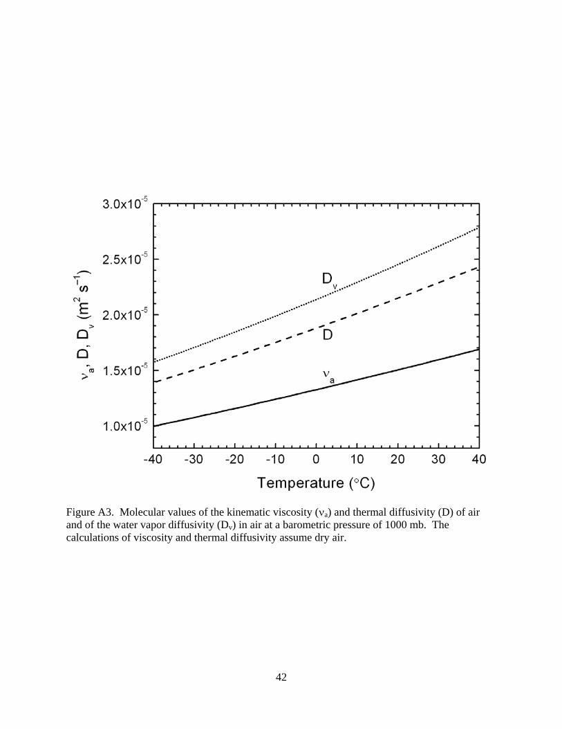
42

Figure A3. Molecular values of the kinematic viscosity (νa) and thermal diffusivity (D) of air and of the water vapor diffusivity (Dv) in air at a barometric pressure of 1000 mb. The calculations of viscosity and thermal diffusivity assume dry air.

43

Figure A4. Effects of surface curvature on the thermal conductivity of air [ ak ' , from (A13.1)] and on the water vapor diffusivity in air [ vD ' , from (A13.3)]. The plot also shows for comparison the unmodified values, ka [from (A11.1)] and Dv [from (A12.1)]. The air temperature is assumed to be 20°C, and the barometric pressure is 1000 mb.