Appendix A Application of Thermocouples in Steady Laminar

Appendix A: Application of Thermocouples in Steady Laminar Flames 111

Appendix A Application of Thermocouples inSteady Laminar Flames

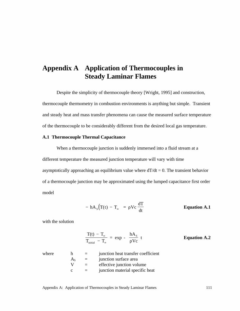
Despite the simplicity of thermocouple theory [Wright, 1995] and construction,

thermocouple thermometry in combustion environments is anything but simple. Transient

and steady heat and mass transfer phenomena can cause the measured surface temperature

of the thermocouple to be considerably different from the desired local gas temperature.

A.1 Thermocouple Thermal Capacitance

When a thermocouple junction is suddenly immersed into a fluid stream at a

different temperature the measured junction temperature will vary with time

asymptotically approaching an equilibrium value where dT/dt = 0. The transient behavior

of a thermocouple junction may be approximated using the lumped capacitance first order

model

( )− − =∞hA VcdT

dtS T(t T) ρ Equation A.1

with the solution

T(t) T

T Texp -

hA

Vcinitial

S−−

=∞

∞ ρ

t Equation A.2

where h = junction heat transfer coefficientAS = junction surface areaV = effective junction volumec = junction material specific heat


ρ = junction material densityt = timeT(t) = junction temperature at time tTinitial = junction temperature at time t = 0T∞ = free stream gas temperature

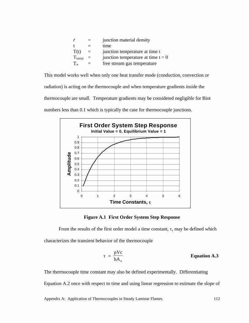
This model works well when only one heat transfer mode (conduction, convection or

radiation) is acting on the thermocouple and when temperature gradients inside the

thermocouple are small. Temperature gradients may be considered negligible for Biot

numbers less than 0.1 which is typically the case for thermocouple junctions.

First Order System Step ResponseInitial Value = 0, Equilibrium Value = 1

0

0.1

0.2

0.3

0.4

0.5

0.6

0.7

0.8

0.9

1

0 1 2 3 4 5 6

Time Constants, ττ

Am

plit

ud

e

Figure A.1 First Order System Step Response

From the results of the first order model a time constant, τ, may be defined which

characterizes the transient behavior of the thermocouple

τρ

=Vc

hAS

Equation A.3

The thermocouple time constant may also be defined experimentally. Differentiating

Equation A.2 once with respect to time and using linear regression to estimate the slope of


− =

τ

d

dtln

T(t) T

T Tinitial

−−

∞

∞

Equation A.4

where the logarithm term of Equation A.4 versus time will be linear for true first order

behavior.

Multiple mode heat transfer involving the thermocouple junction, typically found in

combustion environments, tends to invalidate the first order model because there are

several driving temperature differences, i.e. T∞,conduction, T∞,convection and T∞,radiation. To

effectively model the transient behavior for a thermocouple undergoing multiple modes of

heat transfer it is best to use an implicit model.

A.2 Thermocouple Thermometry in Non-Sooting Flames

It is important to note that thermal equilibrium does not necessarily imply that all

heat transfer involving the junction has ceased but rather the rates of conductive,

convective and radiative heat transfer have become steady with time. Most commonly

when a thermocouple is in thermal equilibrium with a non-sooting combustion

environment heat steadily flows by convection from the surrounding gas into the junction

balanced by lead wire conduction and radiation with cooler surroundings steadily drawing

heat away from the junction as stated in Equation A.5. These heat transfer processes can

cause differences between the thermocouple temperature and the gas temperature of

several hundred Kelvin.

& & &q q qconvection radiation conduction= + Equation A.5


The effects of lead wire conduction can be minimized through the choice of

thermocouple geometry and experiment design. By increasing the length of thermocouple

wire in crossflow to be much larger than the wire diameter conduction effects can be

minimized. Collis and Williams [1959] recommends wire (length / diameter) ≥ 1000 to

thermally isolate the middle of the wire from end effects. Conduction effects may also be

minimized by choosing, whenever possible, to align the length of wire in crossflow along

an isotherm as is commonly done in two dimensional flames such as Tsuji counterflow

burners and Wolfhard-Parker coflowing slot burners. Analytical heat transfer calculations

by Bradley and Matthews [1968] showed that errors due to conduction effects could be

reduced to less than 0.1 % for 12.5 µm uncoated thermocouple wire 5 mm long (length /

diameter = 400) aligned along an isotherm in a flame. Based on their calculations for

coated wires with a final diameter of 100 µm Bradley and Matthews [1968] recommended

doubling the thermocouple length to 10 mm (length / diameter = 100). The remaining

discussion will neglect thermocouple lead wire conduction effects.

Using conservation of energy for a thermocouple in equilibrium with its

surroundings as stated in Equation A.6 and quantitative information about the convection

& &q qconvection radiation= Equation A.6

and radiation heat transfer process one can calculate the difference between the measured

thermocouple temperature and the local gas temperature. With knowledge of the

thermocouple’s radiant emissivity, ε, thermocouple surface temperature and the


temperature of the surroundings one can estimate the radiant heat flux away from the

junction by using Equation A.7

( )′′ = −q T Tradiation tc surrσε 4 4 Equation A.7

where σ = Boltzman constant; 5.67x10-8 W/m2⋅K

Checking the relative magnitudes of the fourth power of the surroundings

temperature versus the fourth power of the thermocouple temperature one might choose

to neglect the surrounding’s temperature term. It is tempting to consider the flame under

investigation as a radiating surface in the temperature correction but analysis usually

shows that laboratory scale flames do not make a significant contribution. Although the

combustion gases and soot particles are at very high temperatures, short mean beam

lengths in laboratory scale flames usually limits their emissivity to < 0.1.

Using empirical correlations to quantify the heat transfer coefficient, h, in the

convective term of Equation A.6

( )′′ = −q h T Tconvection gas tc Equation A.8

where hNu k

dd gas

=⋅

Equation A.9

( )Nu fd d= Re , Pr , empirical correlation Equation A.10

and Nud = Nusselt NumberRed = Reynolds numberPr = Prandtl numberkgas = gas thermal conductivityd = thermocouple junction diameter


Empirical Nusselt number relations exist for flows over various geometries (i.e. spheres,

infinite cylinders…) and the correct expression depends on accurate characterization of

the thermocouple junction geometry. A detailed discussion of typical thermocouple

convection properties is presented later in section A.5. This analysis will proceed under

the assumption that the thermocouple Nusselt number is known. From Equations A.6 -

A.10 the gas temperature may be calculated as

( )T T T Td

Nu kgas tc tc surrd

= + −⋅

σε 4 4 Equation A.11

A.3 Thermocouple Thermometry in Sooting Flames

The preceding analysis for radiation correction to thermocouple measurements in

combustion environments is only valid for non-sooting flames. Thermocouple

thermometry in sooting flames is complicated even further by mass transport of soot from

the gas flow to the thermocouple surface [Eisner and Rosner, 1985]. When a clean

thermocouple is placed into a sooting flame thermophoresis dominates the soot transport

to the thermocouple surface [McEnally et. al., 1997] and is augmented by coagulation and

surface growth reactions identical to those that soot particles in the flow naturally

experience.

Thermophoresis is a diffusion process that tends to drive particles in a temperature

gradient from hot to cold. This process may be easily rationalized by the kinetics of gases

in a temperature gradient. One can imagine that a particle in a temperature gradient will

have more molecular collisions on its hot side than cold side with the resulting


conservation of momentum driving the particle from hot to cold. Since a thermocouple in

thermal equilibrium with a combustion gas stream typically experiences steady convective

heating by the surrounding gas there also must exist a temperature gradient dropping from

the free stream temperature to a lower thermocouple surface temperature. This

convective temperature gradient surrounding the thermocouple is the thermophoretic

driving potential.

With continuous mass transport of soot from the gas stream to the thermocouple

surface affecting the heat transfer process via changes in thermocouple Nusselt number

and radiant emissivity the thermocouple junction never achieves thermal equilibrium with

its surroundings. Transient analysis of thermocouple measurements in sooting flames is

required to determine the gas temperature.

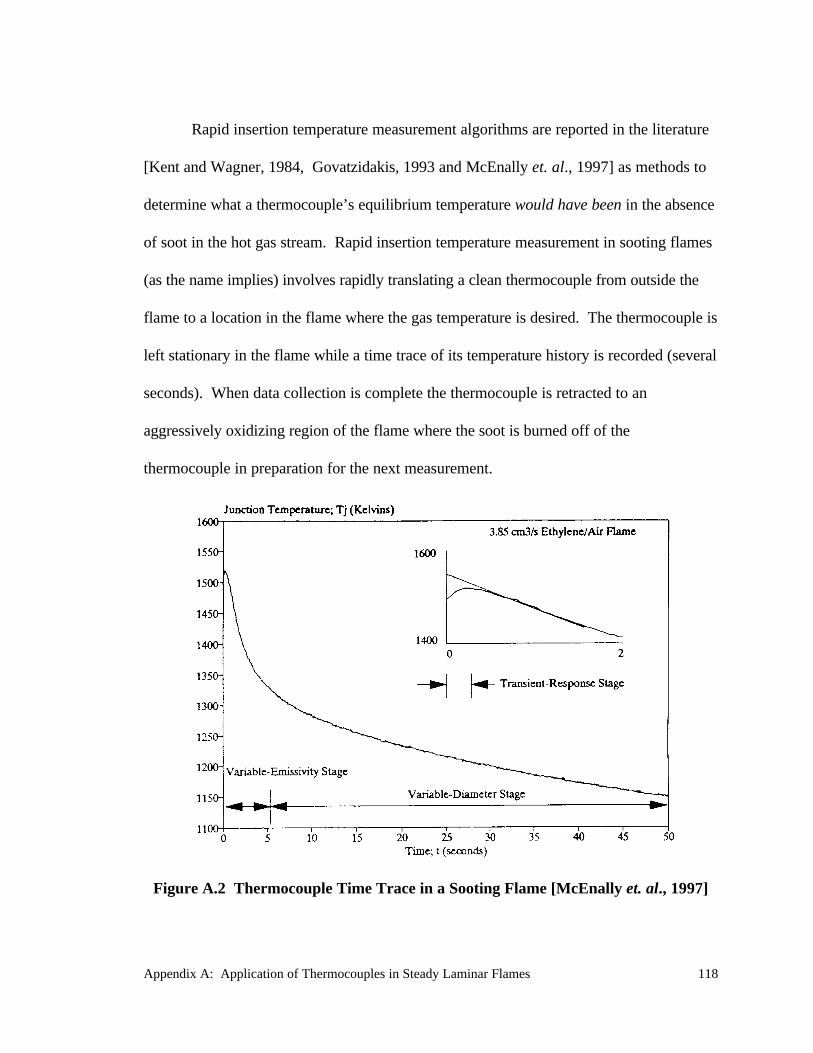
Figure A.2 taken from McEnally et. al. [1997] shows a typical time trace for a

clean thermocouple inserted into a sooting flame. The transient behavior of the

thermocouple is first dominated by its thermal capacitance followed by soot transport

effects. The initial effect of soot deposition on the thermocouple is to gradually change its

radiant emissivity with negligible change to the thermocouple’s diameter. Using platinum

alloy thermocouples their emissivity will vary from approximately 0.2 clean to nearly 1.0

(blackbody) coated with soot. Variations in the thermocouple’s diameter, and therefore

Reynolds number and Nusselt number, from soot deposition dominate the response after

the variable emissivity region. The end of the variable emissivity region and beginning of

the variable diameter region is usually identified by an abrupt change in the slope of the

temperature profile seen in Figure A.2 at about 5 seconds.


Rapid insertion temperature measurement algorithms are reported in the literature

[Kent and Wagner, 1984, Govatzidakis, 1993 and McEnally et. al., 1997] as methods to

determine what a thermocouple’s equilibrium temperature would have been in the absence

of soot in the hot gas stream. Rapid insertion temperature measurement in sooting flames

(as the name implies) involves rapidly translating a clean thermocouple from outside the

flame to a location in the flame where the gas temperature is desired. The thermocouple is

left stationary in the flame while a time trace of its temperature history is recorded (several

seconds). When data collection is complete the thermocouple is retracted to an

aggressively oxidizing region of the flame where the soot is burned off of the

thermocouple in preparation for the next measurement.

Figure A.2 Thermocouple Time Trace in a Sooting Flame [McEnally et. al., 1997]


With the radiant emissivity and convective heat transfer coefficient of the

thermocouple changing in time the only time that these quantities are well known is at the

time of insertion, t = 0. Linear extrapolation of the variable emissivity region of the

temperature profile to time zero (instant of insertion) can be used as an estimate of what

the thermocouple equilibrium temperature would have been in the absence of soot

deposition [Govatzidakis, 1993]. The local gas temperature can now be calculated based

on the “time zero” thermocouple temperature approximation and the clean radiative and

convective heat transfer properties using Equations A.6 - A.11 as discussed previously.

A.4 Thermocouple Particle Densitometry

A technique recently developed by McEnally et. al. [1997] called Thermocouple

Particle Densitometry (TPD) can be used to extract the actual value of the local soot

volume fraction from thermocouple time traces in sooting flames. TPD involves fitting

measured temperature time traces in the variable diameter region to an analytical

thermophoretic transport model yielding local soot volume fraction. Analysis shows that

thermophoresis is the dominant mass transport mechanism for soot deposition on the

thermocouple [McEnally et. al., 1997]. Advantages of this method over optical

absorption techniques is that the measurement is independent of the soot size, morphology

and optical properties and does not require line of sight optical access to implement.

The following is an abbreviated summary of TPD analysis developed in detail in

McEnally et. al. [1997]; the interested reader is encouraged to review the article. By

conservation of energy for a thermocouple junction in quasi-steady equilibrium


( )ε σj tc j

g j

tcgas tc jT

k Nu

dT T, ,

4 0 2 2

2=

⋅− Equation A.12

where j = index indicating jth sample in temperature/time tracekg0 = kg / Tgas = constant value 6.54 x 10-5 W/mK2

Equations A.11 and A.12 express the same idea with the only differences being that

Equation A.12 neglects the surroundings temperature in the radiation term and that the

convection term is stated in terms of heat flux potentials [Rosner, 1986] taking advantage

of the linearity of kg with temperature. Equation A.12 applied to the extrapolated zeroth

data point of the temperature profile as discussed in section A.3 yields an estimate of the

local gas temperature.

The thermophoretic soot mass flux from the free stream to the thermocouple

surface, j″, can be expressed as

( ) ( )′′ = −

j D Nu f d T TT j v P tc j tc j gasρ 2 1

2

, , Equation A.13

where ( )DT mom gas= +−3

41 8

1πα ν Equation A.14

and DT = thermophoretic diffusivityfv = soot volume fractionρP = intrinsic density of soot particlesαmom = momentum accommodation coefficient ≈ 1νgas = gas kinematic viscosity

= 1.29 x 10-9 Tgas1.65 m2/s

By conservation of mass the soot mass flux, j″, can be related to the change in diameter

of either a cylinder or sphere as


( )′′ =j

d d

dtd tc jρ

2

, Equation A.15

where ρd = soot deposit density

It is important to note that the intrinsic density of soot particle in the free stream, ρP, is

different from the soot deposit density, ρd. Measurements by [Choi et. al., 1995] estimate

ρd / ρP = ϕ = 0.095 ± 0.04.

Assuming εj and Nuj to be constant with time during the variable diameter stage

Equation A.12 may be differentiated with respect to time to yield

( ) ( )d d

dt

k NuT T T

dT

dt

tc j g

soottc j gas tc j

tc j,

, ,

,=

−− −0 3 2 52

ε σ Equation A.16

Assuming εj constant at the value of soot emissivity (~0.95) in the variable diameter region

is a very good assumption. Assuming the thermocouple Nusselt number to remain

constant in the variable diameter region is marginal at best but attractive considering the

simplicity it offers. Equations A.12, A.13, A.15 and A.16 are combined to form a

differential equation which may be integrated to yield

( )G mt G t= + = 0 Equation A.17

where GT

T

T

Tgas

tc j

gas

tc j

≡

−

1

4

1

6

8 6

, ,

Equation A.18

m fv≡ ⋅β Equation A.19

( )β ε σ φ≡ 2 2 40

2D T k NuT soot gas g Equation A.20


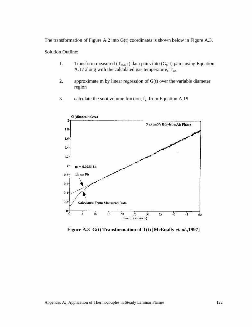
The transformation of Figure A.2 into G(t) coordinates is shown below in Figure A.3.

Solution Outline:

1. Transform measured (Ttc,j, t) data pairs into (Gj, t) pairs using EquationA.17 along with the calculated gas temperature, Tgas

2. approximate m by linear regression of G(t) over the variable diameterregion

3. calculate the soot volume fraction, fv, from Equation A.19

Figure A.3 G(t) Transformation of T(t) [McEnally et. al.,1997]


A.5 Convection Heat Transfer Properties of Thermocouple Junctions

Application of any of the ideas in the previous sections of this appendix require

detailed knowledge of the thermocouple junction’s convective heat transfer

characteristics. Accurate models for the thermocouple’s convective heat transfer

coefficient, h, or Nusselt number, Nud, (h and Nud related by Equation A.9) are needed.

Historically the convective behavior of thermocouple junctions were derived from

empirical relations for infinite cylinders [Whitaker, 1972] or spheres [Collis and Williams,

1959]. The decision of whether a thermocouple junction behaved similar to that of a

cylinder or sphere was typically made based on a visual qualitative judgment of its

junction diameter, dj, relative to the lead wire diameter, dw. Clearly for large dj/dw the

junction would behave much like a sphere and for dj/dw → 1 more like a cylinder.

Empirical convective heat transfer relations typically used to model thermocouple

junctions are shown below in Equations A.21 and A.22.

from Collis and Williams [1959]

[ ]Nu A BRT

Td cylindern m

,

.

= +

∞

0 17

Equation A.21

where T∞ ≡ free stream temperatureTm ≡ “film temperature” = (T∞ + T0) / 2

Table A.1 Values of n, A and B for Equation A.21

0.02 < Red < 44 44 < Red < 140n 0.45 0.51A 0.24 0B 0.56 0.48


from Whitaker [1972]

( ) ( )Nud sphere d d,/ / .. Re . Re Pr= + + ∞2 0 4 0 061 2 2 3 0 4

0µ µ Equation A.22

where µ0 ≡ fluid dynamic viscosity at the junction surface temperatureµ∞ ≡ fluid dynamic viscosity at the free stream temperature

for 0.71 < Pr < 380 3.5 < Red < 7.6 x 104

1.0 < (µ∞/ µ0) < 3.2

All fluid properties in Equation A.21 are evaluated at the film temperature, Tm, and the

properties used in Equation A.22 are evaluated at the free stream temperature, T∞, unless

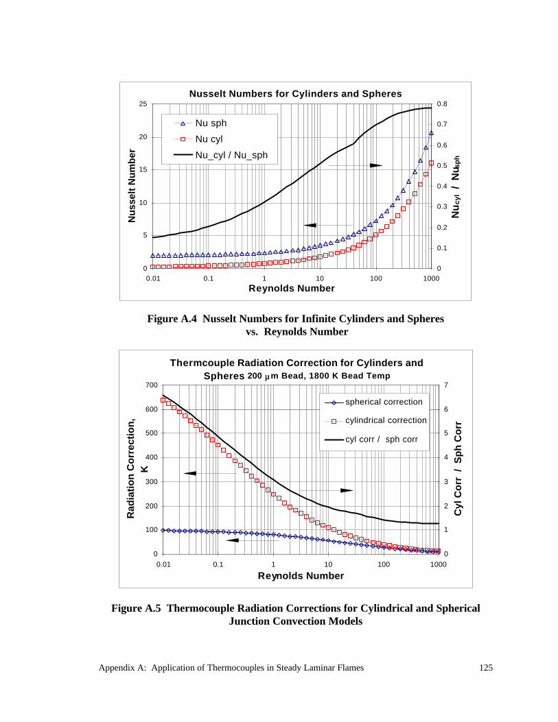
otherwise subscripted. Examining the plots of Equations A.21 and A.22 versus Reynolds

number in Figure A.4, notice that as Red→ 0 (free convection), Nud,cyl→ 0 but Nud,sph→

2.0. The limiting value of Nusselt number for spheres at small Reynolds numbers is not

intuitively obvious but is analytically based [Acrivos and Taylor, 1962] and experimentally

verified [Vliet and Leppert, 1961]. Notice also how the ratio of Nucyl / Nusph rapidly

decreases for small Reynolds numbers further illustrating fundamental differences in the

convection behavior of these two geometries.

From Figure A.5 one can see that for small Reynolds numbers, Red < 10, typical of

laboratory scale laminar flames, the choice of cylindrical versus spherical thermocouple

junction convective heat transfer models can make a difference of hundreds of degrees in

the calculated gas temperatures. The most extreme consequences of these differences are

realized in counterflow flames where the flame front lies near a true stagnation plane, Red


Nusselt Numbers for Cylinders and Spheres

0

5

10

15

20

25

0.01 0.1 1 10 100 1000

Reynolds Number

Nu

ssel

t N

um

ber

0

0.1

0.2

0.3

0.4

0.5

0.6

0.7

0.8

Nu

cyl

/ N

u sp

h

Nu sph

Nu cyl

Nu_cyl / Nu_sph

Figure A.4 Nusselt Numbers for Infinite Cylinders and Spheres vs. Reynolds Number

Thermcouple Radiation Correction for Cylinders and Spheres 200 µµ m Bead, 1800 K Bead Temp

0

100

200

300

400

500

600

700

0.01 0.1 1 10 100 1000

Reynolds Number

Rad

iati

on

Co

rrec

tio

n,

K

0

1

2

3

4

5

6

7

Cyl

Co

rr /

Sp

h C

orr

spherical correction

cylindrical correction

cyl corr / sph corr

Figure A.5 Thermocouple Radiation Corrections for Cylindrical and SphericalJunction Convection Models


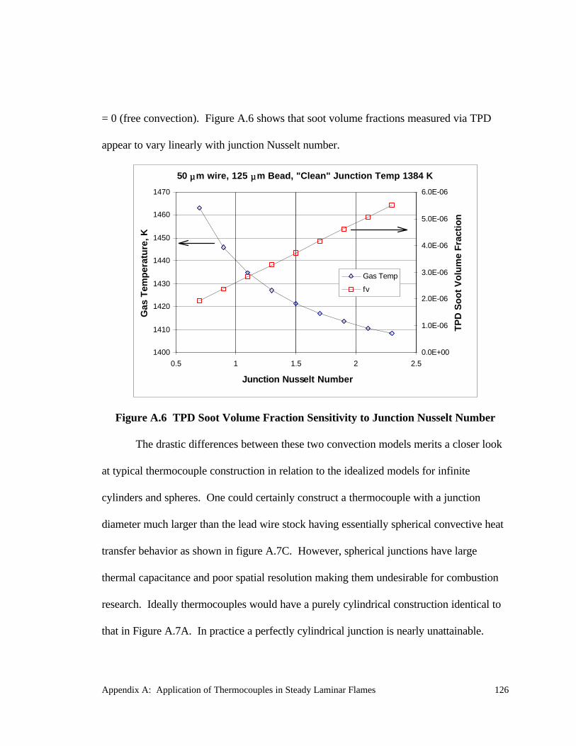
= 0 (free convection). Figure A.6 shows that soot volume fractions measured via TPD

appear to vary linearly with junction Nusselt number.

50 µµm wire, 125 µµm Bead, "Clean" Junction Temp 1384 K

1400

1410

1420

1430

1440

1450

1460

1470

0.5 1 1.5 2 2.5

Junction Nusselt Number

Gas

Tem

per

atu

re, K

0.0E+00

1.0E-06

2.0E-06

3.0E-06

4.0E-06

5.0E-06

6.0E-06

TP

D S

oo

t V

olu

me

Fra

ctio

n

Gas Temp

fv

Figure A.6 TPD Soot Volume Fraction Sensitivity to Junction Nusselt Number

The drastic differences between these two convection models merits a closer look

at typical thermocouple construction in relation to the idealized models for infinite

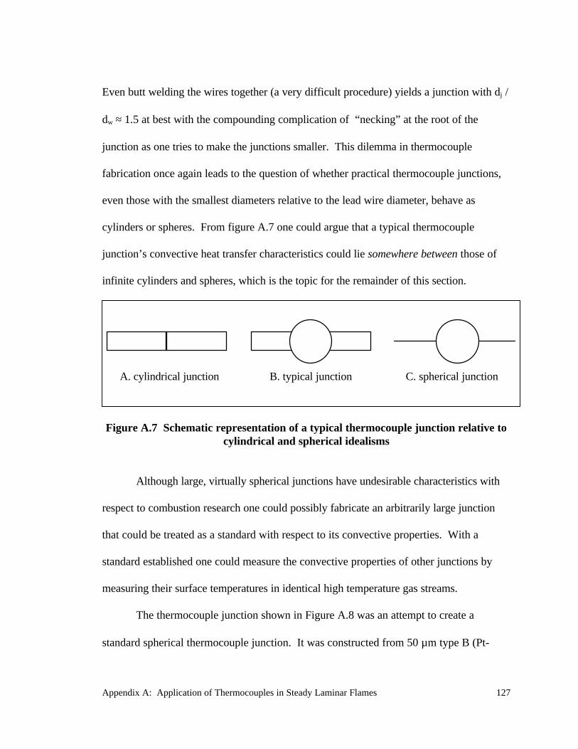
cylinders and spheres. One could certainly construct a thermocouple with a junction

diameter much larger than the lead wire stock having essentially spherical convective heat

transfer behavior as shown in figure A.7C. However, spherical junctions have large

thermal capacitance and poor spatial resolution making them undesirable for combustion

research. Ideally thermocouples would have a purely cylindrical construction identical to

that in Figure A.7A. In practice a perfectly cylindrical junction is nearly unattainable.


Even butt welding the wires together (a very difficult procedure) yields a junction with dj /

dw ≈ 1.5 at best with the compounding complication of “necking” at the root of the

junction as one tries to make the junctions smaller. This dilemma in thermocouple

fabrication once again leads to the question of whether practical thermocouple junctions,

even those with the smallest diameters relative to the lead wire diameter, behave as

cylinders or spheres. From figure A.7 one could argue that a typical thermocouple

junction’s convective heat transfer characteristics could lie somewhere between those of

infinite cylinders and spheres, which is the topic for the remainder of this section.

A. cylindrical junction B. typical junction C. spherical junction

Figure A.7 Schematic representation of a typical thermocouple junction relative tocylindrical and spherical idealisms

Although large, virtually spherical junctions have undesirable characteristics with

respect to combustion research one could possibly fabricate an arbitrarily large junction

that could be treated as a standard with respect to its convective properties. With a

standard established one could measure the convective properties of other junctions by

measuring their surface temperatures in identical high temperature gas streams.

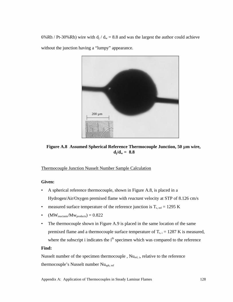
The thermocouple junction shown in Figure A.8 was an attempt to create a

standard spherical thermocouple junction. It was constructed from 50 µm type B (Pt-


6%Rh / Pt-30%Rh) wire with dj / dw = 8.8 and was the largest the author could achieve

without the junction having a “lumpy” appearance.

200 µm

Figure A.8 Assumed Spherical Reference Thermocouple Junction, 50 µµm wire, dj/dw = 8.8

Thermocouple Junction Nusselt Number Sample Calculation

Given:

• A spherical reference thermocouple, shown in Figure A.8, is placed in a

Hydrogen/Air/Oxygen premixed flame with reactant velocity at STP of 8.126 cm/s

• measured surface temperature of the reference junction is Ts, ref = 1295 K

• (MWreactants/Mwproducts) = 0.822

• The thermocouple shown in Figure A.9 is placed in the same location of the same

premixed flame and a thermocouple surface temperature of Ts, i = 1287 K is measured,

where the subscript i indicates the ith specimen which was compared to the reference

Find:

Nusselt number of the specimen thermocouple , Nurel, i, relative to the reference

thermocouple’s Nusselt number Nusph, ref


Assume:

1. perfectly spherical convective behavior for the reference junction

2. premixed flame products properties are identical to that of air at the same temperature

and behave as an ideal gas

3. the hydrogen/air/oxygen premixed flame product’s temperature is sufficiently small to

neglect catalytic effects on the surface of the thermocouples’ junctions [Kaskan,

1957]

Solution:

Conservation of Mass

( )v vMW

MW

T

T

m

s

T

Kproducts reacantsr

p

gas

stp

gas=

=

0 08126 082168

300. .

Conservation of Energy from Equation A.11 for reference junction

( )T T T Td

Nu kgas s ref s ref surrref

sph ref

= + −⋅, ,

,

σε 4 4

Empirical Nusselt number relation from Equation A.22

( ) ( )Nu sph ref d ref d ref, ,/

,/ .. Re . Re Pr= + + ∞2 0 4 0 061 2 2 3 0 4

0µ µ

iterations on Tgas yields:

Tgas = 1361 K vproducts = 30.3 cm/sRed,ref = 0.6868 ε = 0.1945Nusph, ref = 2.3411

Now with a trustworthy estimate of gas temperature calculated based on the

reference thermocouple junction recalculate fluid properties based on specimen

thermocouple film temperature.


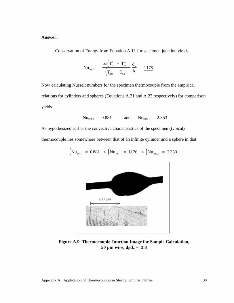
Answer:

Conservation of Energy from Equation A.11 for specimen junction yields

( )( )Nu

T T

T T

d

krel i

s i surr

gas s i

i,

,

,

.=−

−=

σε 4 4

1175

Now calculating Nusselt numbers for the specimen thermocouple from the empirical

relations for cylinders and spheres (Equations A.21 and A.22 respectively) for comparison

yields

Nucyl, i = 0.881 and Nusph, i = 2.353

As hypothesized earlier the convective characteristics of the specimen (typical)

thermocouple lies somewhere between that of an infinite cylinder and a sphere in that

( ) ( ) ( )Nu Nu Nucyl i rel i sph i, , ,. . .= < = < =0881 1176 2 353

200 µm

Figure A.9 Thermocouple Junction Image for Sample Calculation,50 µµm wire, dj/dw = 3.8


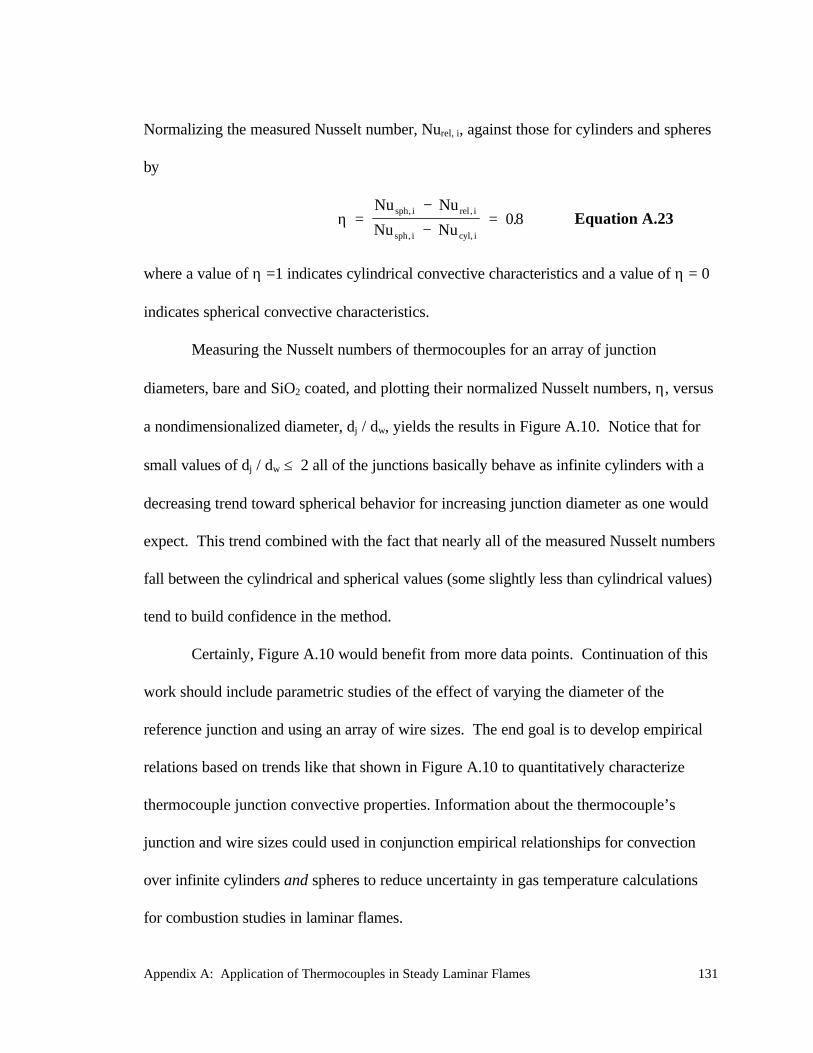
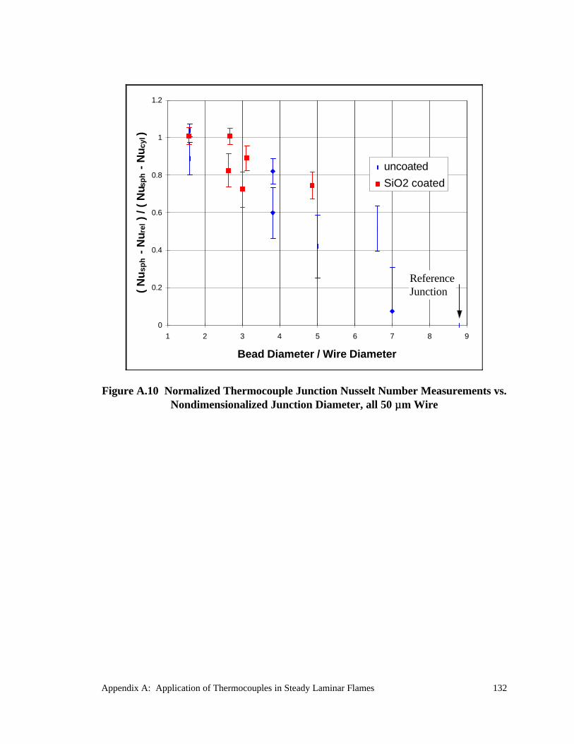
Normalizing the measured Nusselt number, Nurel, i, against those for cylinders and spheres

by

η =−

−=

Nu Nu

Nu Nusph i rel i

sph i cyl i

, ,

, ,

.08 Equation A.23

where a value of η =1 indicates cylindrical convective characteristics and a value of η = 0

indicates spherical convective characteristics.

Measuring the Nusselt numbers of thermocouples for an array of junction

diameters, bare and SiO2 coated, and plotting their normalized Nusselt numbers, η, versus

a nondimensionalized diameter, dj / dw, yields the results in Figure A.10. Notice that for

small values of dj / dw ≤ 2 all of the junctions basically behave as infinite cylinders with a

decreasing trend toward spherical behavior for increasing junction diameter as one would

expect. This trend combined with the fact that nearly all of the measured Nusselt numbers

fall between the cylindrical and spherical values (some slightly less than cylindrical values)

tend to build confidence in the method.

Certainly, Figure A.10 would benefit from more data points. Continuation of this

work should include parametric studies of the effect of varying the diameter of the

reference junction and using an array of wire sizes. The end goal is to develop empirical

relations based on trends like that shown in Figure A.10 to quantitatively characterize

thermocouple junction convective properties. Information about the thermocouple’s

junction and wire sizes could used in conjunction empirical relationships for convection

over infinite cylinders and spheres to reduce uncertainty in gas temperature calculations

for combustion studies in laminar flames.


0

0.2

0.4

0.6

0.8

1

1.2

1 2 3 4 5 6 7 8 9

Bead Diameter / Wire Diameter

( N

usp

h -

Nu r

el )

/ (

Nu s

ph -

Nu

cyl )

uncoated

SiO2 coated

Figure A.10 Normalized Thermocouple Junction Nusselt Number Measurements vs.Nondimensionalized Junction Diameter, all 50 µµm Wire

ReferenceJunction

Documents

Appendix A Application of Thermocouples in Steady Laminar