Embed Size (px)
Citation preview
Appendix A
Answers to End-of-Chapter Practice
Problems
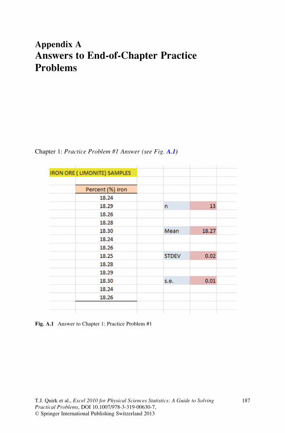
Chapter 1: Practice Problem #1 Answer (see Fig. A.1)
Fig. A.1 Answer to Chapter 1: Practice Problem #1
T.J. Quirk et al., Excel 2010 for Physical Sciences Statistics: A Guide to SolvingPractical Problems, DOI 10.1007/978-3-319-00630-7,© Springer International Publishing Switzerland 2013
187

Chapter 1: Practice Problem #2 Answer (see Fig. A.2)
Fig. A.2 Answer to Chapter 1: Practice Problem #2
188 Appendix A Answers to End-of-Chapter Practice Problems
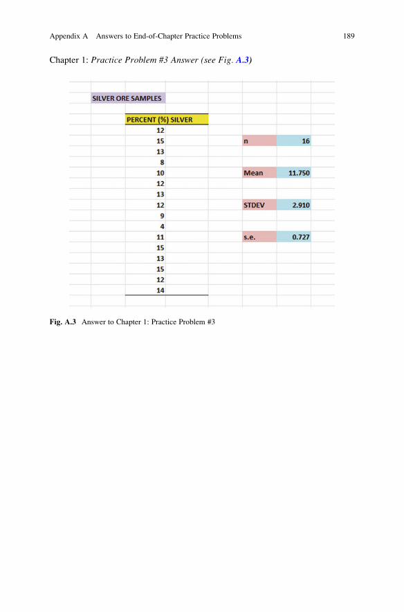
Chapter 1: Practice Problem #3 Answer (see Fig. A.3)
Fig. A.3 Answer to Chapter 1: Practice Problem #3
Appendix A Answers to End-of-Chapter Practice Problems 189

Chapter 2: Practice Problem #1 Answer (see Fig. A.4)
Fig. A.4 Answer to Chapter 2: Practice Problem #1
190 Appendix A Answers to End-of-Chapter Practice Problems
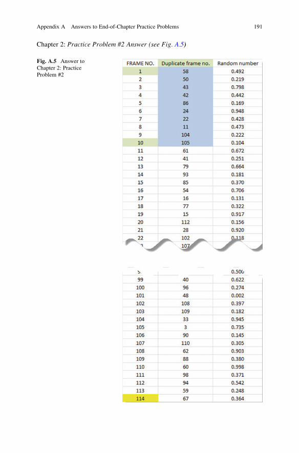
Chapter 2: Practice Problem #2 Answer (see Fig. A.5)
Fig. A.5 Answer to
Chapter 2: Practice
Problem #2
Appendix A Answers to End-of-Chapter Practice Problems 191

Chapter 2: Practice Problem #3 Answer (see Fig. A.6)
Fig. A.6 Answer to Chapter 2: Practice Problem #3
192 Appendix A Answers to End-of-Chapter Practice Problems
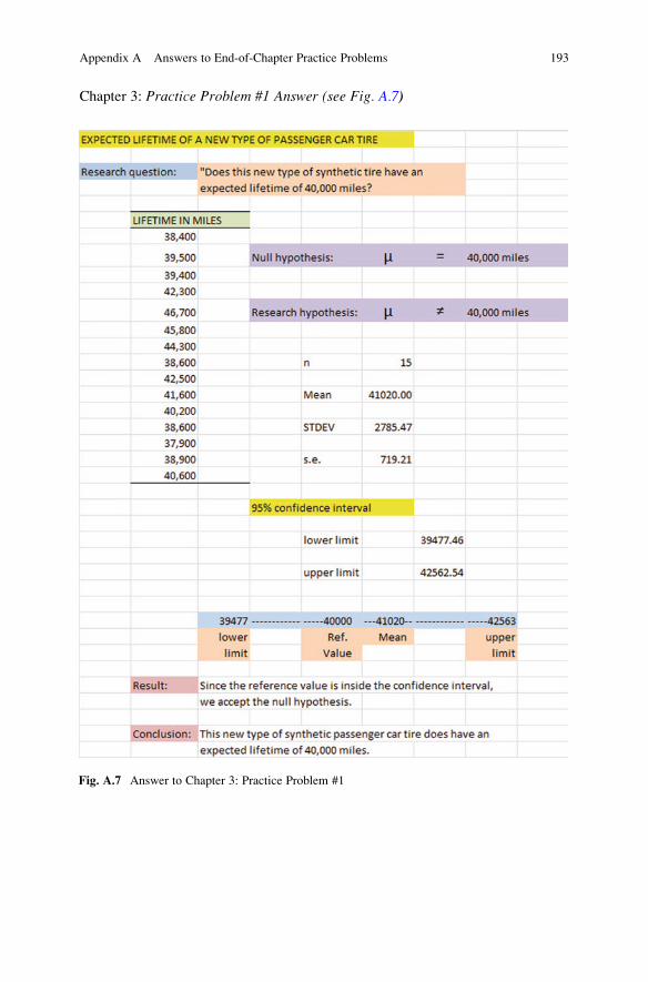
Chapter 3: Practice Problem #1 Answer (see Fig. A.7)
Fig. A.7 Answer to Chapter 3: Practice Problem #1
Appendix A Answers to End-of-Chapter Practice Problems 193
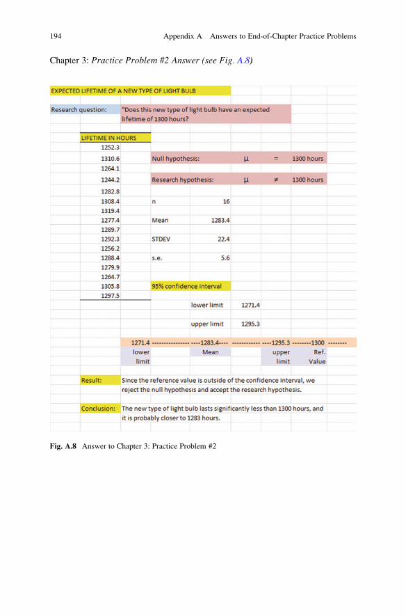
Chapter 3: Practice Problem #2 Answer (see Fig. A.8)
Fig. A.8 Answer to Chapter 3: Practice Problem #2
194 Appendix A Answers to End-of-Chapter Practice Problems
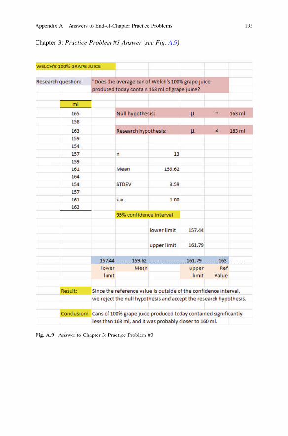
Chapter 3: Practice Problem #3 Answer (see Fig. A.9)
Fig. A.9 Answer to Chapter 3: Practice Problem #3
Appendix A Answers to End-of-Chapter Practice Problems 195
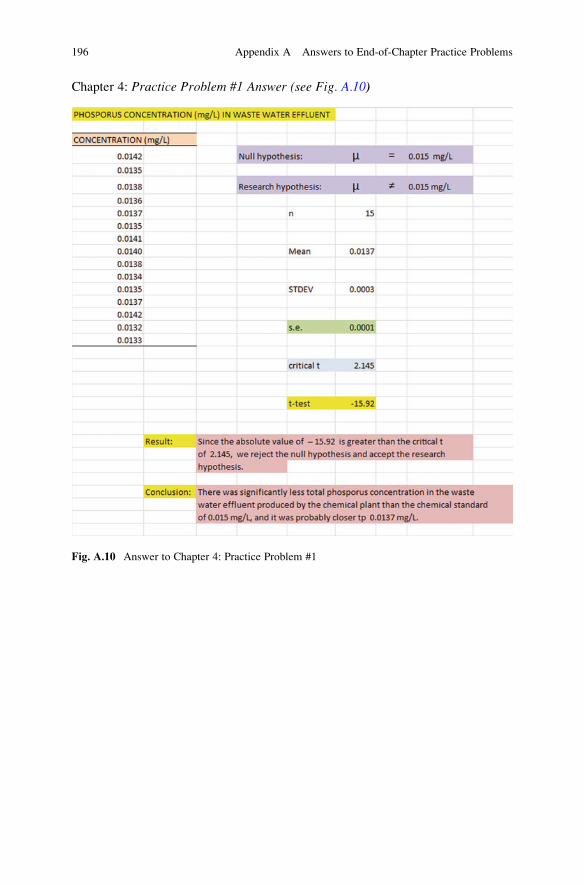
Chapter 4: Practice Problem #1 Answer (see Fig. A.10)
Fig. A.10 Answer to Chapter 4: Practice Problem #1
196 Appendix A Answers to End-of-Chapter Practice Problems

Chapter 4: Practice Problem #2 Answer (see Fig. A.11)
Fig. A.11 Answer to Chapter 4: Practice Problem #2
Appendix A Answers to End-of-Chapter Practice Problems 197

Chapter 4: Practice Problem #3 Answer (see Fig. A.12)
Fig. A.12 Answer to Chapter 4: Practice Problem #3
198 Appendix A Answers to End-of-Chapter Practice Problems

Chapter 5: Practice Problem #1 Answer (see Fig. A.13)
Fig. A.13 Answer to Chapter 5: Practice Problem #1
Appendix A Answers to End-of-Chapter Practice Problems 199
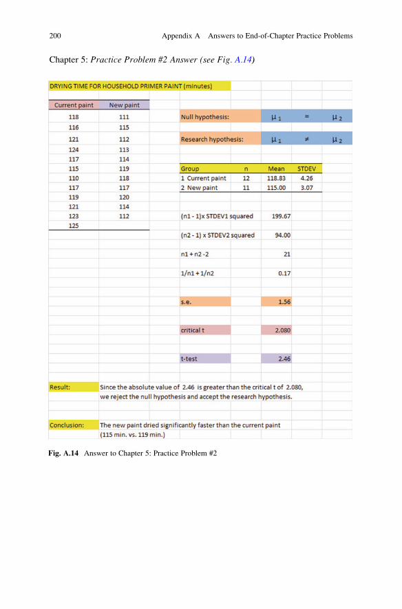
Chapter 5: Practice Problem #2 Answer (see Fig. A.14)
Fig. A.14 Answer to Chapter 5: Practice Problem #2
200 Appendix A Answers to End-of-Chapter Practice Problems
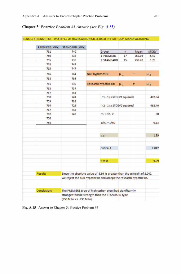
Chapter 5: Practice Problem #3 Answer (see Fig. A.15)
Fig. A.15 Answer to Chapter 5: Practice Problem #3
Appendix A Answers to End-of-Chapter Practice Problems 201
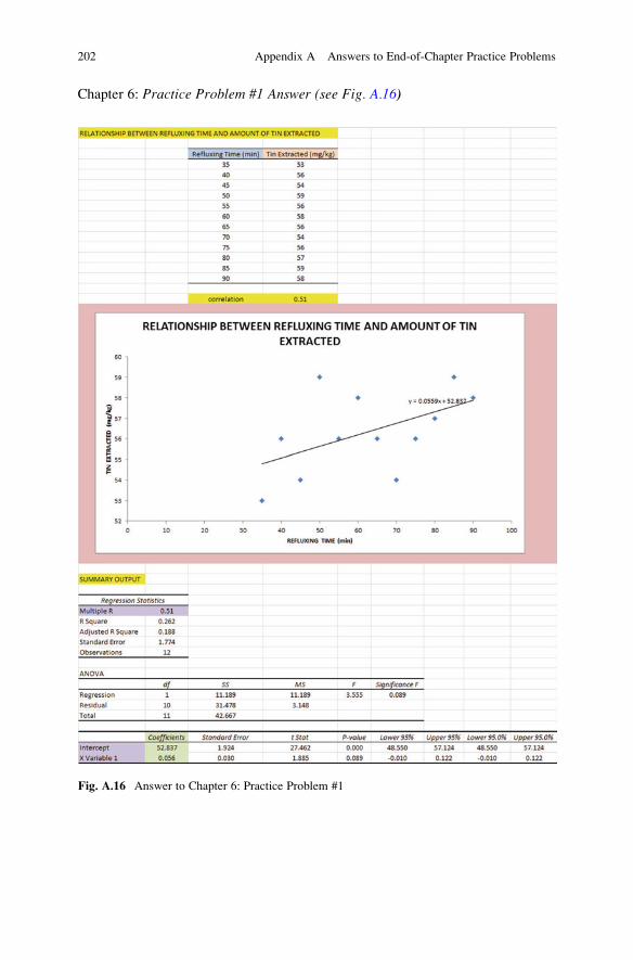
Chapter 6: Practice Problem #1 Answer (see Fig. A.16)
Fig. A.16 Answer to Chapter 6: Practice Problem #1
202 Appendix A Answers to End-of-Chapter Practice Problems

Chapter 6: Practice Problem #1 (continued)
1. r ¼ +.51
2. a ¼ y-intercept ¼ + 52.837
3. b ¼ slope ¼ 0.056
4. Y ¼ a + b X
Y ¼ 52.837 + 0.056 X
5. Y ¼ 52.837 + 0.056 (60)
Y ¼ 52.837 + 3.36
Y ¼ 56.20 mg/kg
Appendix A Answers to End-of-Chapter Practice Problems 203

Chapter 6: Practice Problem #2 Answer (see Fig. A.17)
Fig. A.17 Answer to Chapter 6: Practice Problem #2
204 Appendix A Answers to End-of-Chapter Practice Problems

Chapter 6: Practice Problem #2 (continued)
(2b) about � 1.9 degrees centigrade
1. r ¼ +.94
2. a ¼ y-intercept ¼ �3.43
3. b ¼ slope ¼ + 0.53
4. Y ¼ a + b X
Y ¼ �3.43 + 0.53 X
5. Y ¼ �3.43 + 0.53 (2)
Y ¼ �3.43 + 1.06
Y ¼ �2.37 degrees centigrade
Appendix A Answers to End-of-Chapter Practice Problems 205
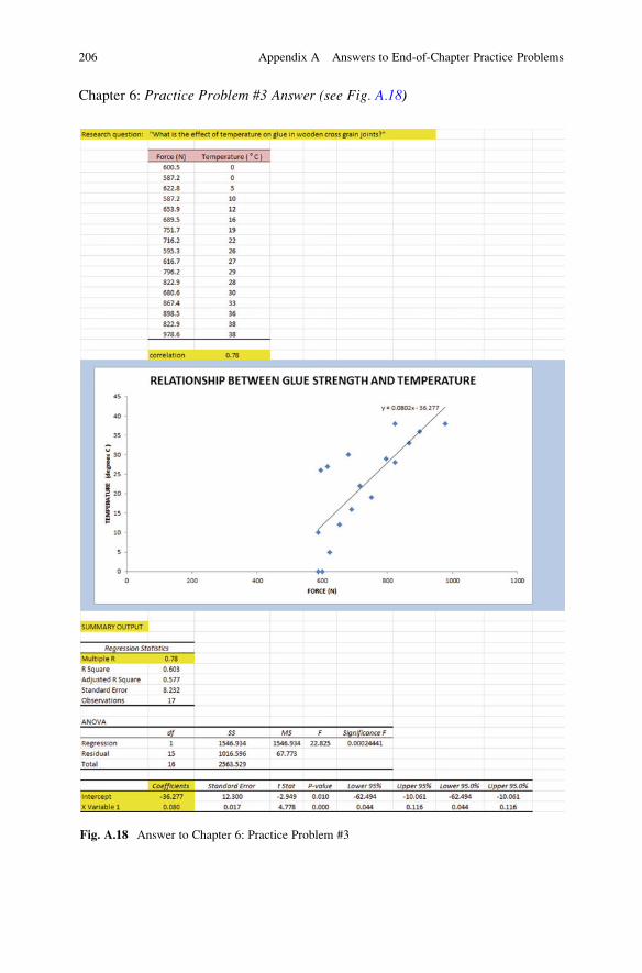
Chapter 6: Practice Problem #3 Answer (see Fig. A.18)
Fig. A.18 Answer to Chapter 6: Practice Problem #3
206 Appendix A Answers to End-of-Chapter Practice Problems
Chapter 6: Practice Problem #3 (continued)
1. r ¼ +.78
2. a ¼ y-intercept ¼ �36.277
3. b ¼ slope ¼ + 0.080
4. Y ¼ a + b X
Y ¼ �36.277 + 0.080 X
5. Y ¼ �36.277 + 0.080 (800)
Y ¼ �36.277 + 64
Y ¼ 27.72 degrees centigrade
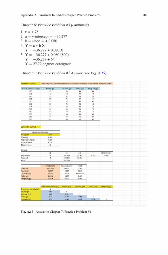
Chapter 7: Practice Problem #1 Answer (see Fig. A.19)
Fig. A.19 Answer to Chapter 7: Practice Problem #1
Appendix A Answers to End-of-Chapter Practice Problems 207

Chapter 7: Practice Problem #1 (continued)
1. Multiple correlation ¼ .74
2. y-intercept ¼ 377.0213
3. b1 ¼ 0.1347
4. b2 ¼ 0.0000
5. b3 ¼ �0.3236
6. b4 ¼ �0.0136
7. Y ¼ a + b 1 X 1 + b 2 X 2 + b3 X3 + b4 X4
Y ¼ 377.0213 + 0.1347 X 1 + 0.0000 X2 � 0.3236 X3 � 0.0136 X4
8. Y ¼ 377.0213 + 0.1347 (63) + 0.0000 (58 ) � 0.3236 (41) � 0.0136 (50)
Y ¼ 377.0213 + 8.49 + 0.0 � 13.27 � 0.68
Y ¼ 371.56
Y ¼ 372 Mpa
9. 0.50
10. 0.37
11. �.71
12. .06
13. .12
14. �.54
15. The best predictor of breech pressure was flake (r ¼ �.71). Remember: Youneed to ignore the negative sign!
16. The four predictors combined predict breech pressure at Rxy ¼ .74, and this is
slightly better than the best single predictor by itself.
208 Appendix A Answers to End-of-Chapter Practice Problems

Chapter 7: Practice Problem #2 Answer (see Fig. A.20)
Fig. A.20 Answer to Chapter 7: Practice Problem #2
Appendix A Answers to End-of-Chapter Practice Problems 209
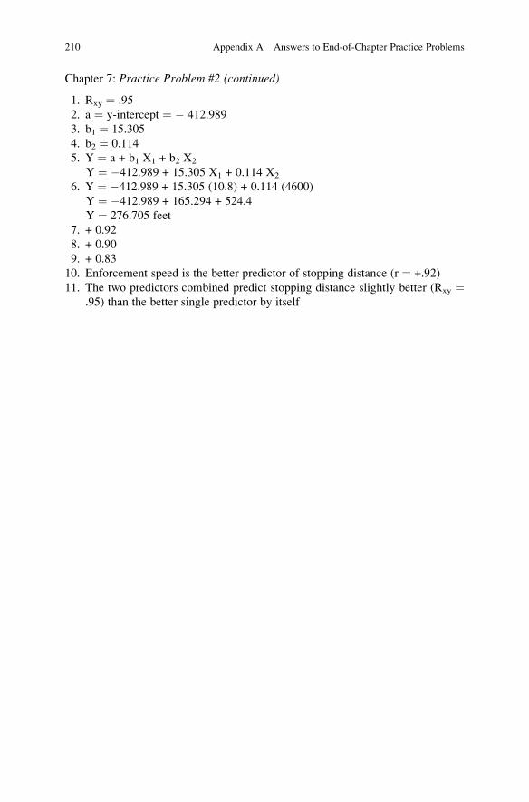
Chapter 7: Practice Problem #2 (continued)
1. Rxy ¼ .95
2. a ¼ y-intercept ¼ � 412.989
3. b1 ¼ 15.305
4. b2 ¼ 0.114
5. Y ¼ a + b1 X1 + b2 X2
Y ¼ �412.989 + 15.305 X1 + 0.114 X2
6. Y ¼ �412.989 + 15.305 (10.8) + 0.114 (4600)
Y ¼ �412.989 + 165.294 + 524.4
Y ¼ 276.705 feet
7. + 0.92
8. + 0.90
9. + 0.83
10. Enforcement speed is the better predictor of stopping distance (r ¼ +.92)
11. The two predictors combined predict stopping distance slightly better (Rxy ¼.95) than the better single predictor by itself
210 Appendix A Answers to End-of-Chapter Practice Problems
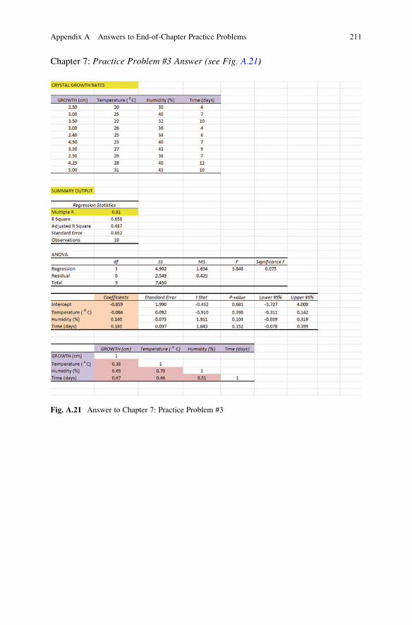
Chapter 7: Practice Problem #3 Answer (see Fig. A.21)
Fig. A.21 Answer to Chapter 7: Practice Problem #3
Appendix A Answers to End-of-Chapter Practice Problems 211
Chapter 7: Practice Problem #3 (continued)
1. Multiple correlation ¼ .81
2. a ¼ y-intercept ¼ �0.859
3. b1 ¼ �0.084
4. b2 ¼ 0.140
5. b3 ¼ 0.160
6. Y ¼ a + b 1 X 1 + b 2 X 2 + b 3 X 3
Y ¼ �0.859 �0.084 X 1 + 0.140 X2 + 0.160 X3
7. Y ¼ �0.859 �0.084 (25) + 0.140 (34) + 0.160 (6)
Y ¼ �0.859 �2.1 + 4.76 + 0.96
Y ¼ 2.76 cm
8. + 0.38
9. + 0.69
10. + 0.67
11. + 0.70
12. + 0.46
13. + 0.51
14. The best single predictor of GROWTH was Humidity ( r ¼ .69).
15. The three predictors combined predict GROWTH at Rxy¼ .81, and this is much
better than the best single predictor by itself.
212 Appendix A Answers to End-of-Chapter Practice Problems
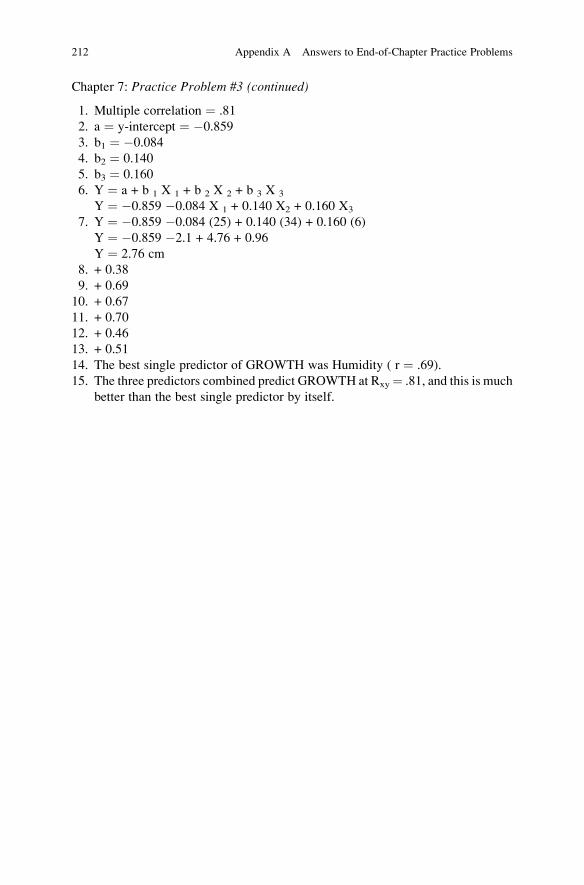
Chapter 8: Practice Problem #1 Answer (see Fig. A.22)
Fig. A.22 Answer to Chapter 8: Practice Problem #1
Appendix A Answers to End-of-Chapter Practice Problems 213

Chapter 8: Practice Problem #1 (continued)Let Group 1 ¼ BELOW ROOM TEMP, Group 2 ¼ ROOM TEMP, and Group
3 ¼ ABOVE ROOM TEMP
1. H0 : μ1 ¼ μ2 ¼ μ3H1 : μ1 6¼ μ2 6¼ μ3
2. MSb ¼ 433.56
3. MSw ¼ 125.44
4. F ¼ 433.56 / 125.44 ¼ 3.46
5. critical F ¼ 3.32
6. Result: Since 3.46 is greater than 3.32, we reject the null hypothesis and accept
the research hypothesis
7. There was a significant difference between the three temperatures in the grams
of product produced.
ROOM TEMP vs. ABOVE ROOM TEMP
8. H0 : μ2 ¼ μ3H1 : μ2 6¼ μ3
9. 83.20
10. 70.64
11. df ¼ 33 �3 ¼ 30
12. critical t ¼ 2.042
13. 1/10 + 1/11 ¼ 0.10 + 0.09 ¼ 0.19
s.e. ¼ SQRT (125.44 * 0.19 ) ¼ SQRT ( 23.83 ) ¼ 4.88
14. ANOVA t ¼ ( 83.20 �70.64 ) / 4.88 ¼ 2.57
15. Result: Since the absolute value of 2.57 is greater than 2.042, we reject the null
hypothesis and accept the research hypothesis
16. Conclusion: ROOM TEMP produced significantly more grams of product than
ABOVE ROOM TEMP (83.2 vs. 70.6).
214 Appendix A Answers to End-of-Chapter Practice Problems
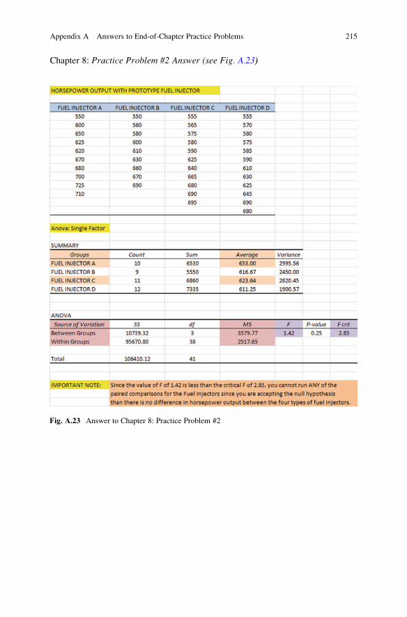
Chapter 8: Practice Problem #2 Answer (see Fig. A.23)
Fig. A.23 Answer to Chapter 8: Practice Problem #2
Appendix A Answers to End-of-Chapter Practice Problems 215

Chapter 8: Practice Problem #2 (continued)
1. Null hypothesis: μA ¼ μB ¼ μC ¼ μDResearch hypothesis: μA 6¼ μB 6¼ μC 6¼ μD
2. MSb ¼ 3579.77
3. MSw ¼ 2517.65
4. F ¼ 3579.77 / 2517.65 ¼ 1.42
5. Critical F ¼ 2.85
6. Since the F-value of 1.42 is less than the critical F value of 2.85, we accept the
null hypothesis.
7. There was no difference between the four types of fuel injectors in their
horsepower output.
8. 8 – 16. Be careful here! You need to remember that it is incorrect to perform
ANY ANOVA t-test when the value of F is less than the critical value of F. The
ANOVA F-test found no difference between the four types of fuel injectors in
horsepower output, and, therefore, you cannot compare any two injectors usingthe ANOVA t-test!
216 Appendix A Answers to End-of-Chapter Practice Problems

Chapter 8: Practice Problem #3 Answer (see Fig. A.24)
Fig. A.24 Answer to Chapter 8: Practice Problem #3
Appendix A Answers to End-of-Chapter Practice Problems 217

Chapter 8: Practice Problem #3 (continued)Let SUBCOMPACTS ¼ Group 1, COMPACTS ¼ Group 2, MID-SIZE ¼
Group 3, LARGE ¼ Group 4, and SUVs ¼ Group 5
1. Null hypothesis: μ1 ¼ μ2 ¼ μ3 ¼ μ4 ¼ μ5Research hypothesis: μ1 6¼ μ2 6¼ μ3 6¼ μ4 6¼ μ5
2. MSb ¼ 179.56
3. MSw ¼ 4.01
4. F ¼ 179.56 / 4.01 ¼ 44.78
5. critical F ¼ 2.63
6. Result: Since the F-value of 44.78 is greater than the critical F value of 2.63, we
reject the null hypothesis and accept the research hypothesis.
7. Conclusion: There was a significant difference between the five types of
vehicles in their highway miles per gallon.
8. Null hypothesis: μ2 ¼ μ4Research hypothesis: μ2 6¼ μ4
9. 29.41
10. 23.73
11. degrees of freedom ¼ 42 �5 ¼ 37
12. critical t ¼ 2.026
13. s.e.ANOVA ¼ SQRT( MS w x {1/9 + 1/10}) ¼ SQRT (4.01 x 0.21) ¼ SQRT
(0.84) ¼ 0.92
14. ANOVA t ¼ (29.41 �23.73) / .92 ¼ 6.17
15. Since the absolute value of 6.17 is greater than the critical t of 2.026, we reject
the null hypothesis and accept the research hypothesis.
16. COMPACTS had significantly higher highway mpg than LARGE vehicles
(29.4 vs. 23.7)
218 Appendix A Answers to End-of-Chapter Practice Problems

Appendix B
Practice Test
Chapter 1: Practice Test
Suppose that you were hired as a research assistant on a project involving concrete
blocks, and that your responsibility on this team was to measure the compressive
strength in units of 100 pounds per square inch (psi) of concrete blocks from a
certain supplier. You want to try out your Excel skills on a small random sample of
blocks. The hypothetical data is given below (see Fig. B.1).
Fig. B.1 Worksheet Data for Chapter 1 Practice Test (Practical Example)
T.J. Quirk et al., Excel 2010 for Physical Sciences Statistics: A Guide to SolvingPractical Problems, DOI 10.1007/978-3-319-00630-7,© Springer International Publishing Switzerland 2013
219
(a) Create an Excel table for these data, and then use Excel to the right of the table
to find the sample size, mean, standard deviation, and standard error of the mean
for these data. Label your answers, and round off the mean, standard deviation,
and standard error of the mean to two decimal places.
(b) Save the file as: CONCRETE3
Chapter 2: Practice Test
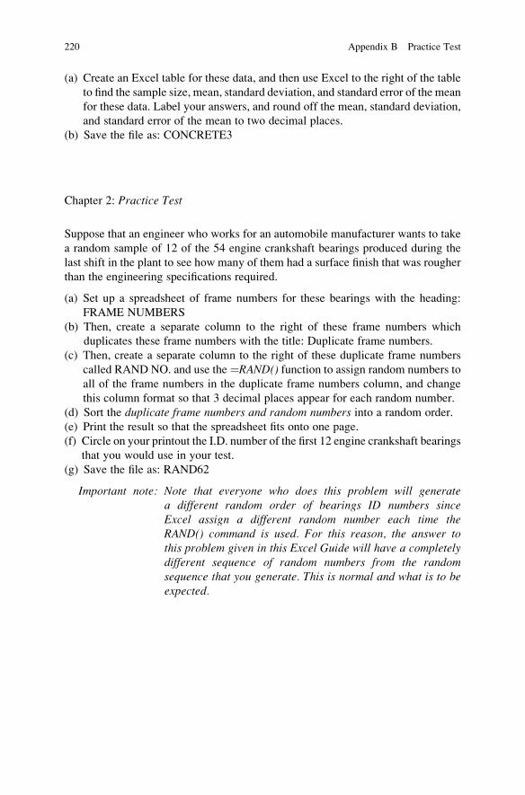
Suppose that an engineer who works for an automobile manufacturer wants to take
a random sample of 12 of the 54 engine crankshaft bearings produced during the
last shift in the plant to see how many of them had a surface finish that was rougher
than the engineering specifications required.
(a) Set up a spreadsheet of frame numbers for these bearings with the heading:
FRAME NUMBERS
(b) Then, create a separate column to the right of these frame numbers which
duplicates these frame numbers with the title: Duplicate frame numbers.
(c) Then, create a separate column to the right of these duplicate frame numbers
called RAND NO. and use the ¼RAND() function to assign random numbers to
all of the frame numbers in the duplicate frame numbers column, and change
this column format so that 3 decimal places appear for each random number.
(d) Sort the duplicate frame numbers and random numbers into a random order.
(e) Print the result so that the spreadsheet fits onto one page.
(f) Circle on your printout the I.D. number of the first 12 engine crankshaft bearings
that you would use in your test.
(g) Save the file as: RAND62
Important note: Note that everyone who does this problem will generatea different random order of bearings ID numbers sinceExcel assign a different random number each time theRAND() command is used. For this reason, the answer tothis problem given in this Excel Guide will have a completelydifferent sequence of random numbers from the randomsequence that you generate. This is normal and what is to beexpected.
220 Appendix B Practice Test

Chapter 3: Practice Test
Suppose that a manufacturer of a certain type of house paint has a factory that
produced an average of 60 tons per day over the past month for this paint. Suppose,
further, that this factory tries out a new manufacturing process for this type of paint
for 30 days. You have been asked to “run the data” to see if any change has occurred
in the production output with this new procedure, and you have decided to test your
Excel skills on a random sample of hypothetical data given in Fig. B.2
(a) Create an Excel table for these data, and use Excel to the right of the table to
find the sample size, mean, standard deviation, and standard error of the mean
for these data. Label your answers, and round off the mean, standard deviation,
and standard error of the mean to two decimal places in number format.
(b) By hand, write the null hypothesis and the research hypothesis on your printout.
(c) Use Excel’s TINV function to find the 95% confidence interval about the mean
for these data. Label your answers. Use two decimal places for the confidence
interval figures in number format.
(d) On your printout, draw a diagram of this 95% confidence interval by hand,
including the reference value.
Fig. B.2 Worksheet Data
for Chapter 3 Practice Test
(Practical Example)
Appendix B Practice Test 221
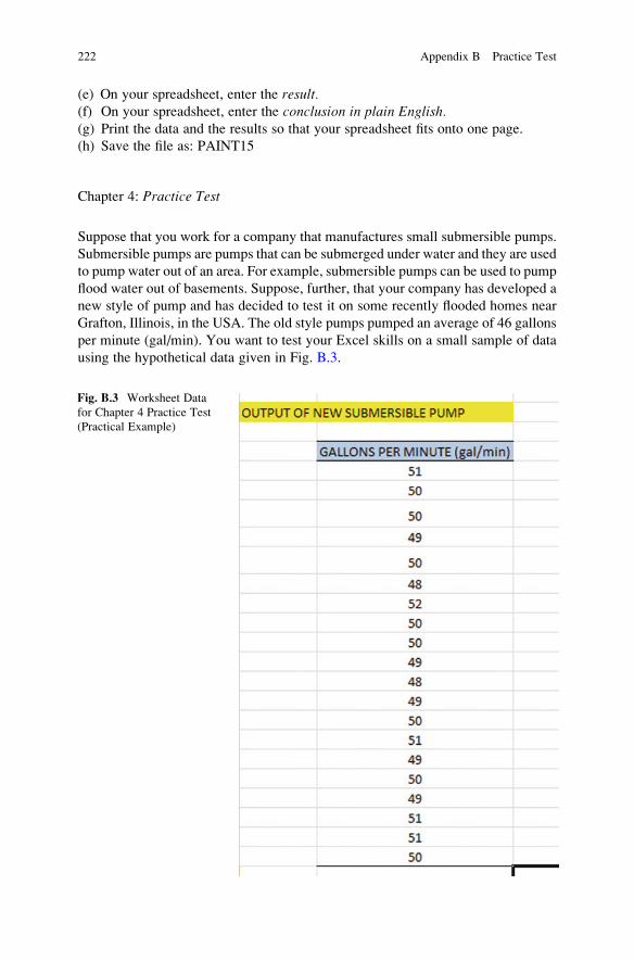
(e) On your spreadsheet, enter the result.(f) On your spreadsheet, enter the conclusion in plain English.(g) Print the data and the results so that your spreadsheet fits onto one page.
(h) Save the file as: PAINT15
Chapter 4: Practice Test
Suppose that you work for a company that manufactures small submersible pumps.
Submersible pumps are pumps that can be submerged under water and they are used
to pump water out of an area. For example, submersible pumps can be used to pump
flood water out of basements. Suppose, further, that your company has developed a
new style of pump and has decided to test it on some recently flooded homes near
Grafton, Illinois, in the USA. The old style pumps pumped an average of 46 gallons
per minute (gal/min). You want to test your Excel skills on a small sample of data
using the hypothetical data given in Fig. B.3.
Fig. B.3 Worksheet Data
for Chapter 4 Practice Test
(Practical Example)
222 Appendix B Practice Test

(a) Write the null hypothesis and the research hypothesis on your spreadsheet.
(b) Create a spreadsheet for these data, and then use Excel to find the sample size,
mean, standard deviation, and standard error of the mean to the right of the data
set. Use number format (2 decimal places) for the mean, standard deviation, and
standard error of the mean.
(c) Type the critical t from the t-table in Appendix E onto your spreadsheet, and
label it.
(d) Use Excel to compute the t-test value for these data (use 2 decimal places) and
label it on your spreadsheet.
(e) Type the result on your spreadsheet, and then type the conclusion in plainEnglish on your spreadsheet.
(f) Save the file as: PUMP8
Chapter 5: Practice Test
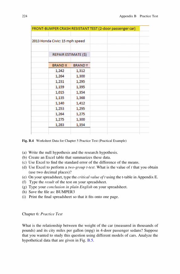
Suppose that an automobile repair parts manufacturer/supplier wants to test the
crash resistance of two brands of front-bumpers for 2-door passenger sedans
(BRAND X and BRAND Y). The engineer in charge of this project has decided
to test these bumpers on 2013 Honda Civics that are purposely crashed into a
cement wall at a speed of 15 miles per hour (mph), and then to estimate the cost of
repairs to the front bumper after this test. The engineer then wants to test her Excel
skills on the hypothetical data given in Fig. B.4.
Appendix B Practice Test 223
(a) Write the null hypothesis and the research hypothesis.
(b) Create an Excel table that summarizes these data.
(c) Use Excel to find the standard error of the difference of the means.
(d) Use Excel to perform a two-group t-test. What is the value of t that you obtain
(use two decimal places)?
(e) On your spreadsheet, type the critical value of t using the t-table in Appendix E.(f) Type the result of the test on your spreadsheet.
(g) Type your conclusion in plain English on your spreadsheet.
(h) Save the file as: BUMPER3
(i) Print the final spreadsheet so that it fits onto one page.
Chapter 6: Practice Test
What is the relationship between the weight of the car (measured in thousands of
pounds) and its city miles per gallon (mpg) in 4-door passenger sedans? Suppose
that you wanted to study this question using different models of cars. Analyze the
hypothetical data that are given in Fig. B.5.
Fig. B.4 Worksheet Data for Chapter 5 Practice Test (Practical Example)
224 Appendix B Practice Test
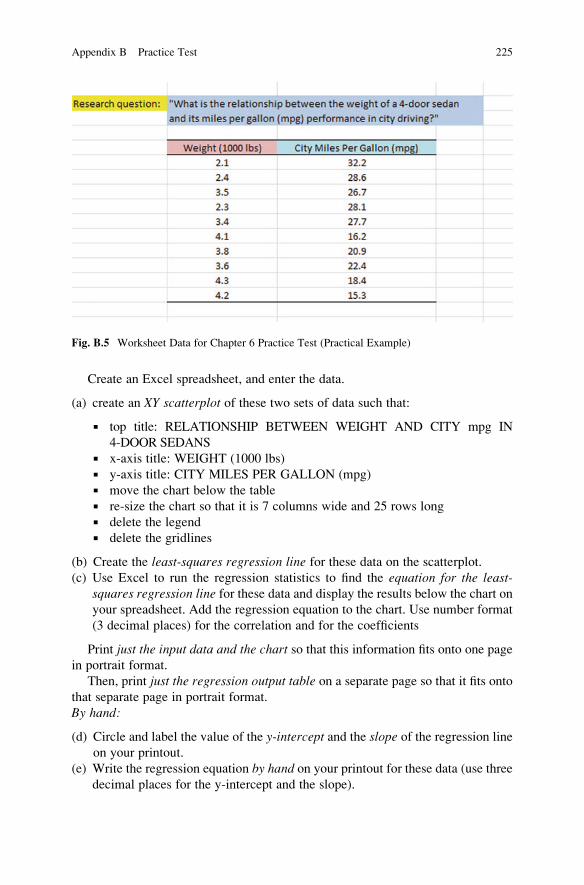
Create an Excel spreadsheet, and enter the data.
(a) create an XY scatterplot of these two sets of data such that:
▪ top title: RELATIONSHIP BETWEEN WEIGHT AND CITY mpg IN
4-DOOR SEDANS
▪ x-axis title: WEIGHT (1000 lbs)
▪ y-axis title: CITY MILES PER GALLON (mpg)
▪ move the chart below the table
▪ re-size the chart so that it is 7 columns wide and 25 rows long
▪ delete the legend
▪ delete the gridlines
(b) Create the least-squares regression line for these data on the scatterplot.
(c) Use Excel to run the regression statistics to find the equation for the least-squares regression line for these data and display the results below the chart on
your spreadsheet. Add the regression equation to the chart. Use number format
(3 decimal places) for the correlation and for the coefficients
Print just the input data and the chart so that this information fits onto one page
in portrait format.
Then, print just the regression output table on a separate page so that it fits onto
that separate page in portrait format.
By hand:
(d) Circle and label the value of the y-intercept and the slope of the regression line
on your printout.
(e) Write the regression equation by hand on your printout for these data (use threedecimal places for the y-intercept and the slope).
Fig. B.5 Worksheet Data for Chapter 6 Practice Test (Practical Example)
Appendix B Practice Test 225
(f) Circle and label the correlation between the two sets of scores in the regressionanalysis summary output table on your printout.
(g) Underneath the regression equation you wrote by hand on your printout, use the
regression equation to predict the average city mpg of a 4-door sedan that
weighted 2,500 pounds.
(h) Read from the graph, the average city mpg you would predict for a 4-door sedan
that weighed 3,600 pounds, and write your answer in the space immediately
below:________________________
(i) save the file as: sedan3
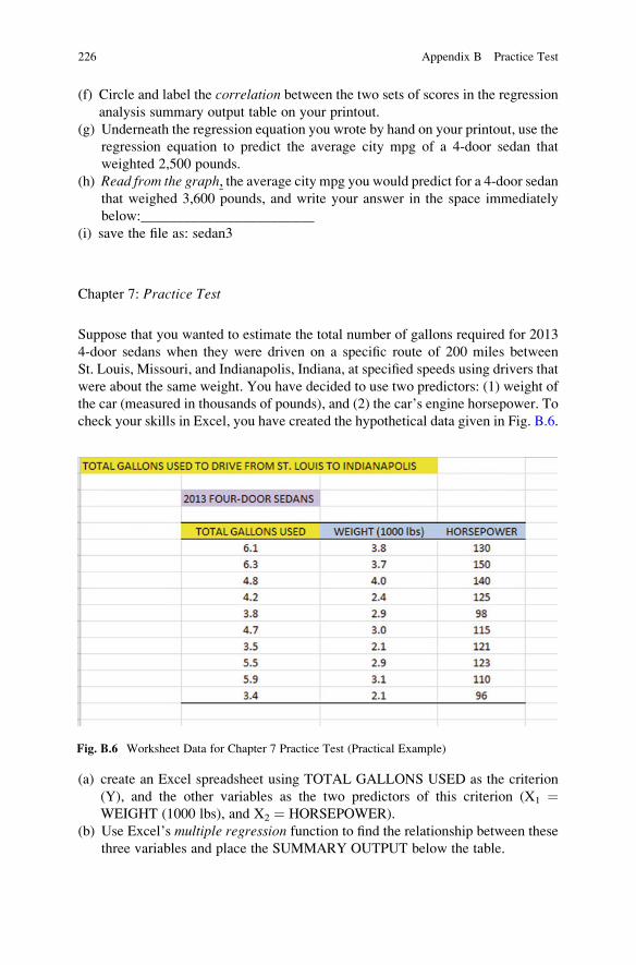
Chapter 7: Practice Test
Suppose that you wanted to estimate the total number of gallons required for 2013
4-door sedans when they were driven on a specific route of 200 miles between
St. Louis, Missouri, and Indianapolis, Indiana, at specified speeds using drivers that
were about the same weight. You have decided to use two predictors: (1) weight of
the car (measured in thousands of pounds), and (2) the car’s engine horsepower. To
check your skills in Excel, you have created the hypothetical data given in Fig. B.6.
(a) create an Excel spreadsheet using TOTAL GALLONS USED as the criterion
(Y), and the other variables as the two predictors of this criterion (X1 ¼WEIGHT (1000 lbs), and X2 ¼ HORSEPOWER).
(b) Use Excel’s multiple regression function to find the relationship between these
three variables and place the SUMMARY OUTPUT below the table.
Fig. B.6 Worksheet Data for Chapter 7 Practice Test (Practical Example)
226 Appendix B Practice Test
(c) Use number format (2 decimal places) for the multiple correlation on the
Summary Output, and use two decimal places for the coefficients in the
SUMMARY OUTPUT.
(d) Save the file as: GALLONS9
(e) Print the table and regression results below the table so that they fit onto
one page.
Answer the following questions using your Excel printout:
1. What is the multiple correlation Rxy ?
2. What is the y-intercept a ?
3. What is the coefficient for WEIGHT b1 ?4. What is the coefficient for HORSEPOWER b2 ?5. What is the multiple regression equation?
6. Predict the TOTAL GALLONS USED you would expect for a WEIGHT of
3,800 pounds and a car that had 126 HORSEPOWER.
(f) Now, go back to your Excel file and create a correlation matrix for these three
variables, and place it underneath the SUMMARY OUTPUT.
(g) Re-save this file as: GALLONS9
(h) Now, print out just this correlation matrix on a separate sheet of paper.
Answer to the following questions using your Excel printout. (Be sure to include
the plus or minus sign for each correlation):
7. What is the correlation between WEIGHT and TOTAL GALLONS USED?
8. What is the correlation between HORSEPOWER and TOTAL GALLONS
USED?
9. What is the correlation between WEIGHT and HORSEPOWER?
10. Discuss which of the two predictors is the better predictor of total
gallons used.
11. Explain in words how much better the two predictor variables combined
predict total gallons used than the better single predictor by itself.
Chapter 8: Practice Test
Let’s consider an experiment in which you want to compare the strength of beams
made of three types of materials: (1) steel, (2) Alloy A, and (3) Alloy B. The
strength of the material was measured by placing each beam in a horizontal position
with a support on each end, and then applying a force of 2,500 pounds to the center
of each beam. The “deflection of the beam” was then measured in 1/1000th of an
inch. You decide to test your Excel skills on a small sample of beams, and you have
created the hypothetical data given in Fig. B.7.
Appendix B Practice Test 227
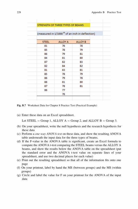
(a) Enter these data on an Excel spreadsheet.
Let STEEL ¼ Group 1, ALLOY A ¼ Group 2, and ALLOY B ¼ Group 3.
(b) On your spreadsheet, write the null hypothesis and the research hypothesis for
these data
(c) Perform a one-way ANOVA test on these data, and show the resulting ANOVA
table underneath the input data for the three types of beams.
(d) If the F-value in the ANOVA table is significant, create an Excel formula to
compute the ANOVA t-test comparing the STEEL beams versus the ALLOY A
beams, and show the results below the ANOVA table on the spreadsheet (put
the standard error and the ANOVA t-test value on separate lines of your
spreadsheet, and use two decimal places for each value)
(e) Print out the resulting spreadsheet so that all of the information fits onto one
page
(f) On your printout, label by hand the MS (between groups) and the MS (within
groups)
(g) Circle and label the value for F on your printout for the ANOVA of the input
data
Fig. B.7 Worksheet Data for Chapter 8 Practice Test (Practical Example)
228 Appendix B Practice Test

(h) Label by hand on the printout the mean for steel beams and the mean for Alloy
A beams that were produced by your ANOVA formulas
(i) Save the spreadsheet as: STRENGTH3
On a separate sheet of paper, now do the following by hand:
(j) find the critical value of F in the ANOVA Single Factor results table
(k) write a summary of the result of the ANOVA test for the input data
(l) write a summary of the conclusion of the ANOVA test in plain English for the
input data
(m) write the null hypothesis and the research hypothesis comparing steel beams
versus Alloy A beams.
(n) compute the degrees of freedom for the ANOVA t-test by hand for three types
of beams.
(o) use your calculator and Excel to compute the standard error (s.e.) of the
ANOVA t-test
(p) Use your calculator and Excel to compute the ANOVA t-test value
(q) write the critical value of t for the ANOVA t-test using the table in Appendix E.
(r) write a summary of the result of the ANOVA t-test
(s) write a summary of the conclusion of the ANOVA t-test in plain English
Appendix B Practice Test 229

Appendix C
Answers to Practice Test
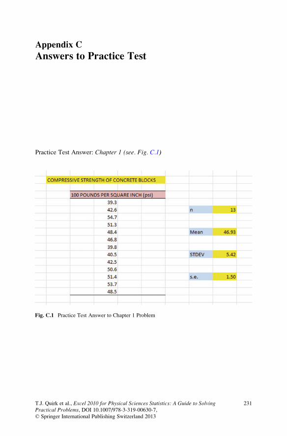
Practice Test Answer: Chapter 1 (see. Fig. C.1)
Fig. C.1 Practice Test Answer to Chapter 1 Problem
T.J. Quirk et al., Excel 2010 for Physical Sciences Statistics: A Guide to SolvingPractical Problems, DOI 10.1007/978-3-319-00630-7,© Springer International Publishing Switzerland 2013
231

Practice Test Answer: Chapter 2 (see. Fig. C.2)
Fig. C.2 Practice Test
Answer to Chapter 2 Problem
232 Appendix C Answers to Practice Test

Practice Test Answer: Chapter 3 (see. Fig. C.3)
Fig. C.3 Practice Test Answer to Chapter 3 Problem
Appendix C Answers to Practice Test 233

Practice Test Answer: Chapter 4 (see. Fig. C.4)
Fig. C.4 Practice Test Answer to Chapter 4 Problem
234 Appendix C Answers to Practice Test

Practice Test Answer: Chapter 5 (see. Fig. C.5)
Fig. C.5 Practice Test Answer to Chapter 5 Problem
Appendix C Answers to Practice Test 235
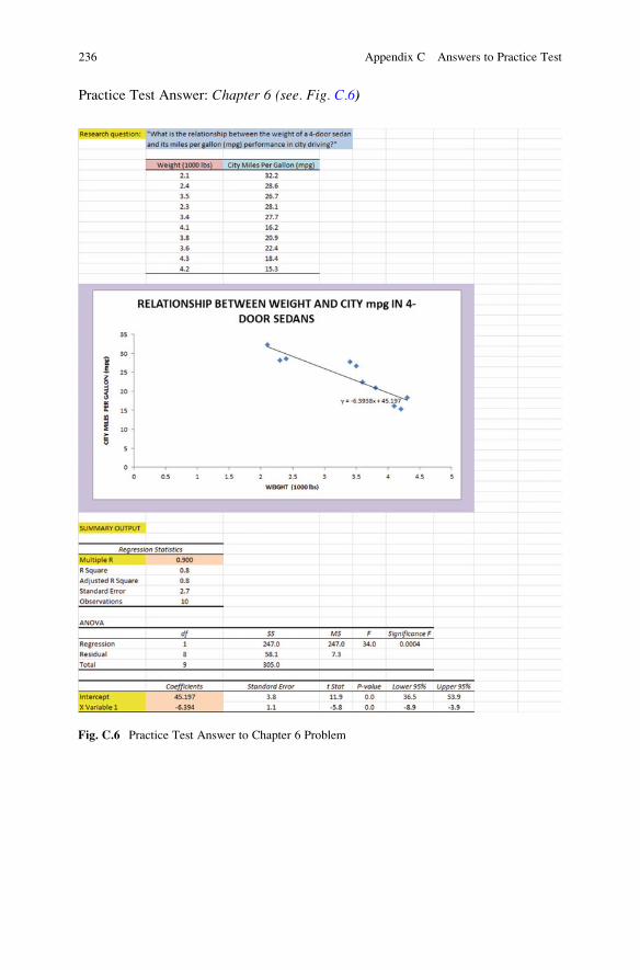
Practice Test Answer: Chapter 6 (see. Fig. C.6)
Fig. C.6 Practice Test Answer to Chapter 6 Problem
236 Appendix C Answers to Practice Test

Practice Test Answer: Chapter 6: (continued)
(d) a ¼ y-intercept ¼ 45.197
b ¼ slope ¼ �6.394 (note the negative sign!)
(e) Y ¼ a + b X
Y ¼ 45.197 �6.394 X
(f) r ¼ correlation ¼ �.900 (note the negative sign!)
(g) Y ¼ 45.197 �6.394 (2.5)
Y ¼ 45.197 �15.985
Y ¼ 29.212 mpg
(h) About 22 – 23 mpg
Appendix C Answers to Practice Test 237
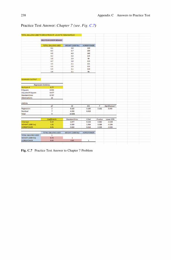
Practice Test Answer: Chapter 7 (see. Fig. C.7)
Fig. C.7 Practice Test Answer to Chapter 7 Problem
238 Appendix C Answers to Practice Test
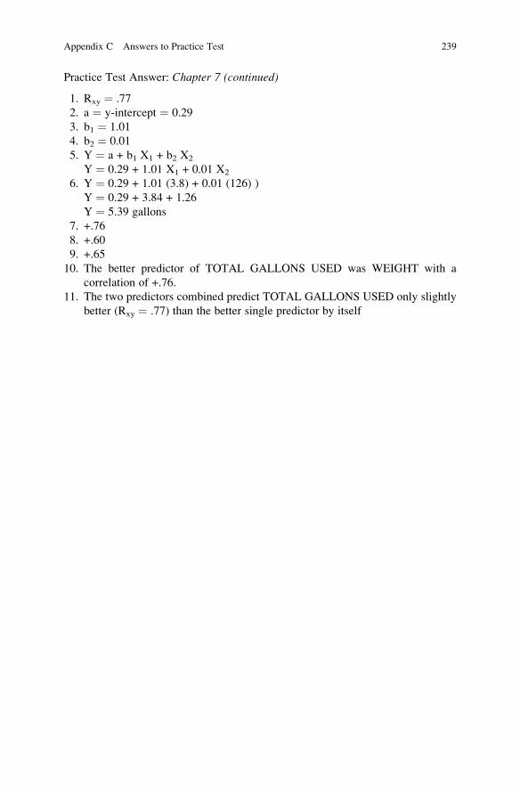
Practice Test Answer: Chapter 7 (continued)
1. Rxy ¼ .77
2. a ¼ y-intercept ¼ 0.29
3. b1 ¼ 1.01
4. b2 ¼ 0.01
5. Y ¼ a + b1 X1 + b2 X2
Y ¼ 0.29 + 1.01 X1 + 0.01 X2
6. Y ¼ 0.29 + 1.01 (3.8) + 0.01 (126) )
Y ¼ 0.29 + 3.84 + 1.26
Y ¼ 5.39 gallons
7. +.76
8. +.60
9. +.65
10. The better predictor of TOTAL GALLONS USED was WEIGHT with a
correlation of +.76.
11. The two predictors combined predict TOTAL GALLONS USED only slightly
better (Rxy ¼ .77) than the better single predictor by itself
Appendix C Answers to Practice Test 239

Practice Test Answer: Chapter 8 (see. Fig. C.8)
Fig. C.8 Practice Test Answer to Chapter 8 Problem
240 Appendix C Answers to Practice Test
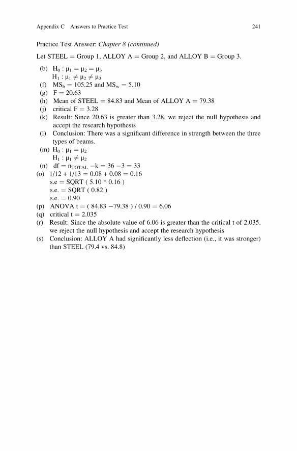
Practice Test Answer: Chapter 8 (continued)
Let STEEL ¼ Group 1, ALLOY A ¼ Group 2, and ALLOY B ¼ Group 3.
(b) H0 : μ1 ¼ μ2 ¼ μ3H1 : μ1 6¼ μ2 6¼ μ3
(f) MSb ¼ 105.25 and MSw ¼ 5.10
(g) F ¼ 20.63
(h) Mean of STEEL ¼ 84.83 and Mean of ALLOY A ¼ 79.38
(j) critical F ¼ 3.28
(k) Result: Since 20.63 is greater than 3.28, we reject the null hypothesis and
accept the research hypothesis
(l) Conclusion: There was a significant difference in strength between the three
types of beams.
(m) H0 : μ1 ¼ μ2H1 : μ1 6¼ μ2
(n) df ¼ nTOTAL �k ¼ 36 �3 ¼ 33
(o) 1/12 + 1/13 ¼ 0.08 + 0.08 ¼ 0.16
s.e ¼ SQRT ( 5.10 * 0.16 )
s.e. ¼ SQRT ( 0.82 )
s.e. ¼ 0.90
(p) ANOVA t ¼ ( 84.83 �79.38 ) / 0.90 ¼ 6.06
(q) critical t ¼ 2.035
(r) Result: Since the absolute value of 6.06 is greater than the critical t of 2.035,
we reject the null hypothesis and accept the research hypothesis
(s) Conclusion: ALLOY A had significantly less deflection (i.e., it was stronger)
than STEEL (79.4 vs. 84.8)
Appendix C Answers to Practice Test 241

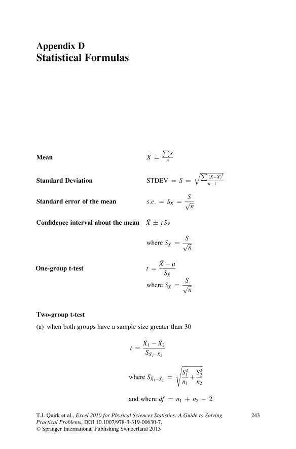
Appendix D
Statistical Formulas
Mean �X ¼P
X
n
Standard Deviation STDEV ¼ S ¼ffiffiffiffiffiffiffiffiffiffiffiffiffiffiffiffiffiP
ðX� �XÞ2n�1
q
Standard error of the mean s:e: ¼ S �X ¼ Sffiffiffin
p
Confidence interval about the mean �X � t S �X
where S �X ¼ Sffiffiffin
p
One-group t-test t ¼�X � μ
S �X
where S �X ¼ Sffiffiffin
p
Two-group t-test
(a) when both groups have a sample size greater than 30
t ¼�X1 � �X2
S �X1� �X2
where S �X1� �X2¼
ffiffiffiffiffiffiffiffiffiffiffiffiffiffiffiS21n1
þ S22n2
s
and where df ¼ n1 þ n2 � 2
T.J. Quirk et al., Excel 2010 for Physical Sciences Statistics: A Guide to SolvingPractical Problems, DOI 10.1007/978-3-319-00630-7,© Springer International Publishing Switzerland 2013
243
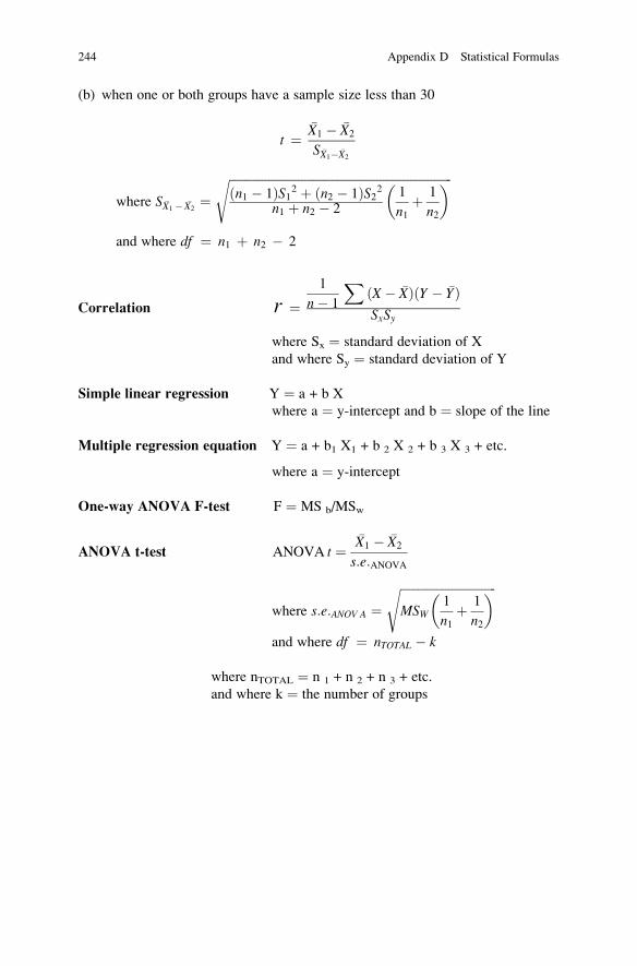
(b) when one or both groups have a sample size less than 30
t ¼�X1 � �X2
S �X1� �X2
where S �X1 � �X2¼
ffiffiffiffiffiffiffiffiffiffiffiffiffiffiffiffiffiffiffiffiffiffiffiffiffiffiffiffiffiffiffiffiffiffiffiffiffiffiffiffiffiffiffiffiffiffiffiffiffiffiffiffiffiffiffiffiffiffiffiffiffiffiffiffiffiffiffiffiffiffiffiffiffiffiðn1 � 1ÞS12 þ ðn2 � 1ÞS22
n1 þ n2 � 21
n1þ 1
n2
� �s
and where df ¼ n1 þ n2 � 2
Correlation r ¼1
n� 1
XðX � �XÞðY � �YÞSxSy
where Sx ¼ standard deviation of X
and where Sy ¼ standard deviation of Y
Simple linear regression Y ¼ a + b X
where a ¼ y-intercept and b ¼ slope of the line
Multiple regression equation Y ¼ a + b1 X1 + b 2 X 2 + b 3 X 3 + etc.
where a ¼ y-intercept
One-way ANOVA F-test F ¼ MS b/MSw
ANOVA t-test ANOVA t ¼�X1 � �X2
s:e:ANOVA
where s:e:ANOV A ¼ffiffiffiffiffiffiffiffiffiffiffiffiffiffiffiffiffiffiffiffiffiffiffiffiffiffiffiffiffiffiffiffiMSW
1
n1þ 1
n2
� �s
and where df ¼ nTOTAL � k
where nTOTAL ¼ n 1 + n 2 + n 3 + etc.
and where k ¼ the number of groups
244 Appendix D Statistical Formulas

Appendix E
t-Table
Critical t-values needed for rejection of the null hypothesis (see Fig. E.1)
T.J. Quirk et al., Excel 2010 for Physical Sciences Statistics: A Guide to SolvingPractical Problems, DOI 10.1007/978-3-319-00630-7,© Springer International Publishing Switzerland 2013
245
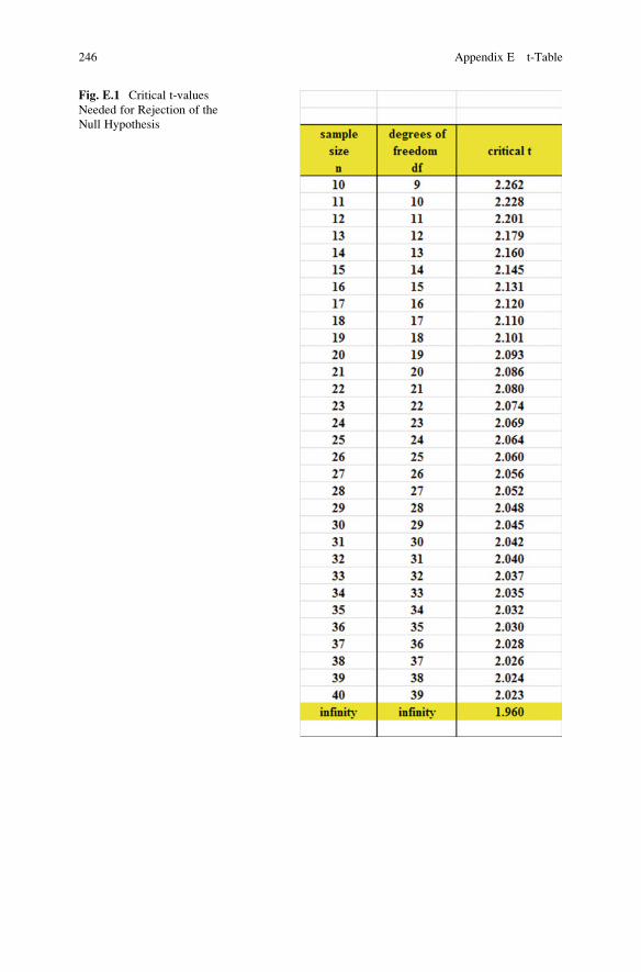
Fig. E.1 Critical t-values
Needed for Rejection of the
Null Hypothesis
246 Appendix E t-Table
Index
A
Absolute value of a number, 68–69
Analysis of variance (ANOVA)
ANOVA t-test formula (8.2), 176
degrees of freedom, 177
Excel commands, 178–180
formula (8.1), 174
interpreting the summary table, 174
s.e. formula for ANOVA t-test (8.3), 176
t-test, 175–180
ANOVA. See Analysis of varianceAverage function. See Mean
C
Centering information within cells, 6–8
Chart
adding the regression equation, 142–144
changing the width and height, 119
creating a chart, 123–132
drawing the regression line onto the
chart, 123–132
moving the chart, 128–129
printing the spreadsheet, 133–134
reducing the scale, 133
scatter chart, 125
titles, 127
Column width (changing), 5–6, 155
Confidence interval about the mean
95% confident, 38–42, 44, 48
drawing a picture, 46
formula (3.2), 41–42, 55
lower limit, 38–39
upper limit, 38–39
Correlation
formula (6.1), 116
negative correlation, 145
positive correlation, 111–113
9 steps for computing, 116–118
CORREL function. See CorrelationCOUNT function, 9–10
Critical t-value, 61, 177, 178
D
Data Analysis ToolPak, 135–137, 153, 169
Data/sort commands, 27
Degrees of freedom, 87–90, 92, 103, 177
F
Fill/series/columns commands, 4–5
step value/stop value commands, 5
Formatting numbers
currency format, 15–16
decimal format, 11–12
H
Home/fill/series commands, 4
Hypothesis testing
decision rule, 55
null hypothesis, 51–54
rating scale hypotheses, 51–54
research hypothesis, 51–54
stating the conclusion, 56–60
stating the result, 60–61
7 steps for hypothesis testing, 54–60
M
Mean, 1–19, 37–65, 67–81, 83–110, 115,
116, 120, 121, 169, 174
formula (1.1), 1
T.J. Quirk et al., Excel 2010 for Physical Sciences Statistics: A Guide to SolvingPractical Problems, DOI 10.1007/978-3-319-00630-7,© Springer International Publishing Switzerland 2013
247
Multiple correlation
correlation matrix, 160–163
Excel commands, 156–159
Multiple regression
correlation matrix, 160–163
equation (7.1), (7.2), 153
Excel commands, 156–159
predicting Y, 153
N
Naming a range of cells, 8–9
Null hypothesis. See Hypothesis testing
O
One-group t-test for the mean
absolute value of a number, 68–69
formula (4.1), 69
hypothesis testing, 67
s.e. formula (4.2), 69
7 steps for hypothesis testing, 67–71
P
Page Layout/Scale to Fit commands, 31,
47, 133
Population mean, 37–38, 40, 51–53, 67,
69, 86, 93, 169, 174–176, 178
Printing a spreadsheet
entire worksheet, 48–49, 75, 99
part of the worksheet, 145–147
printing a worksheet to fit onto one
page, 31–33, 133–134
R
RAND(). See Random number generator
Random number generator
duplicate frame numbers, 24–26
frame numbers, 21–23
sorting duplicate frame numbers
Regression, 123–132
Regression equation
adding it to the chart, 142–144
formula (6.3), 142
negative correlation, 145
predicting Y from x, 141–142
slope, b, 140writing the regression equation
using the Summary Output,
137–140
y-intercept, a, 140–142Regression line, 123–134, 140–144, 150
Research hypothesis. See Hypothesis testing
S
Sample size, 1–19, 39, 41–43, 46, 47, 50,
55, 63–65, 67, 70, 72, 78–80, 83,
86, 87, 89, 92–107, 109, 115, 116,
121, 171, 177
COUNT function, 9–10, 55
Saving a spreadsheet, 13–14
Scale to Fit commands, 31, 47
s.e. See Standard error of the mean
Standard deviation (STDEV), 1–19, 38,
39, 43, 47, 55, 64, 65, 67, 69, 72,
78–80, 84–85, 89, 90, 93–95, 103,
108, 109, 121
formula (1.2), 2
Standard error of the mean (s.e.), 1–19,
38–40, 42, 43, 47, 55, 63–65, 67,
69, 74, 78–80, 93
formula (1.3), 3
STDEV. See Standard deviation
T
t-table. See Appendix E
Two-group t-test
basic table, 85
degrees of freedom, 87–88
drawing a picture of the means, 91
formula (5.2), 92
Formula #1 (5.3), 92
Formula #2 (5.5), 103
hypothesis testing, 83
s.e. formula (5.3), (5.5), 92, 103
9 steps in hypothesis testing, 84–88
248 Index


![54968550 Practice Problems for Chapter 6 With Answers 1[1]](https://img.pdfslide.us/doc/110x75/54e7e8e54a7959d76d8b48bb/54968550-practice-problems-for-chapter-6-with-answers-11.jpg)


![Practice Problems for Chapter 6 With Answers[1]](https://img.pdfslide.us/doc/110x75/5478da66b4af9fb9158b469d/practice-problems-for-chapter-6-with-answers1.jpg)