Appendix A: A VHDL Overview - Springer978-3-319-41198-9/1.pdf · Appendix A: A VHDL Overview ... variable Increment : integer; signal Clk : bit :¼ ‘1’; Constants and variables

Appendix A: A VHDL Overview

This appendix collects the very basics of VHDL language (Very High Speed Integrated Circuits

Hardware Description Language) with the goal of providing enough knowledge to read and under-

stand its usage throughout this book and start developing basic hardware models. This appendix

intends to teach by examples; consequently, most of them will be related to the modules and topics

already addressed in the different chapters of this book.

There are plenty of books and webs available for further VHDL learning, for example Ashenden

(1996), Teres et al. (1998), Ashenden and Lewis (2008), and Kafig (2011).

A.1 Introduction to Hardware Description Languages

The current hardware description languages (HDLs) were developed in the 1980s in order to manage

the growing complexity of very-large-scale integrated circuits (VLSI). Their main objectives are:

• Formal hardware description and modelling

• Verification of hardware descriptions by means of their computer simulation

• Implementation of hardware descriptions by means of their synthesis into physical devices or

systems

Current HDLs share some important characteristics:

• Technology independent: They can describe hardware functionality, but not its detailed imple-

mentation on a specific technology.

• Human and computer readable: They are easy to understand and share.

• Ability to model the inherent concurrent hardware behavior.

• Shared concepts and features with high-level structured software languages like C, C++, or ADA.

Hardware languages are expected to model functionalities that once synthesized will produce

physical processing devices, while software languages describe functions that once compiled will

produce code for specific processors.

Languages which attempt to describe or model hardware systems have been developed at

academic level for a long time, but none of them succeeded until the second half of the 1980s.

# Springer International Publishing Switzerland 2017

J.-P. Deschamps et al., Digital Systems, DOI 10.1007/978-3-319-41198-9189

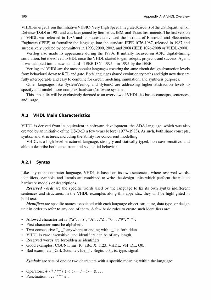
VHDLemerged from the initiativeVHSIC (VeryHighSpeed IntegratedCircuit) of theUSDepartment of

Defense (DoD) in 1981 andwas later joined by Itermetics, IBM, and Texas Instruments. The first version

of VHDL was released in 1985 and its success convinced the Institute of Electrical and Electronics

Engineers (IEEE) to formalize the language into the standard IEEE 1076-1987, released in 1987 and

successively updated by committees in 1993, 2000, 2002, and 2008 (IEEE 1076-2008 or VHDL-2008).

Verilog also made its appearance during the 1980s. It initially focused on ASIC digital-timing

simulation, but it evolved to HDL once the VHDL started to gain adepts, projects, and success. Again,

it was adopted into a new standard—IEEE 1364-1995—in 1995 by the IEEE.

Verilog andVHDLare themost popular languages covering the same circuit design abstraction levels

frombehavioral down toRTL and gate. Both languages shared evolutionary paths and right now they are

fully interoperable and easy to combine for circuit modeling, simulation, and synthesis purposes.

Other languages like SystemVerilog and SytemC are addressing higher abstraction levels to

specify and model more complex hardware/software systems.

This appendix will be exclusively devoted to an overview of VHDL, its basics concepts, sentences,

and usage.

A.2 VHDL Main Characteristics

VHDL is derived from its equivalent in software development, the ADA language, which was also

created by an initiative of the US-DoD a few years before (1977–1983). As such, both share concepts,

syntax, and structures, including the ability for concurrent modelling.

VHDL is a high-level structured language, strongly and statically typed, non-case sensitive, and

able to describe both concurrent and sequential behaviors.

A.2.1 Syntax

Like any other computer language, VHDL is based on its own sentences, where reserved words,

identifiers, symbols, and literals are combined to write the design units which perform the related

hardware models or descriptions.

Reserved words are the specific words used by the language to fix its own syntax indifferent

sentences and structures. In the VHDL examples along this appendix, they will be highlighted in

bold text.

Identifiers are specific names associated with each language object, structure, data type, or design

unit in order to refer to any one of them. A few basic rules to create such identifiers are:

• Allowed character set is {“a”. . .“z”, “A”. . .“Z”, “0”. . .“9”, “_”}.

• First character must be alphabetic.

• Two consecutive “_ _” anywhere or ending with “_” is forbidden.

• VHDL is case insensitive, and identifiers can be of any length.

• Reserved words are forbidden as identifiers.

• Good examples: COUNT, En_10, aBc, X, f123, VHDL, VH_DL, Q0.

• Bad examples: _Ctrl, 2counter, En__1, Begin, q0_, is, type, signal.

Symbols are sets of one or two characters with a specific meaning within the language:

• Operators: + - * / ** ( ) < > ¼ /¼ >¼ & . . .• Punctuation: . , : ‘’ “” # ;

190 Appendix A: A VHDL Overview

• Part of expressions or sentences: ¼> :¼ /¼ >¼ <¼ |

• Comments: -- after this symbol, the remaining text until the end of the line will be considered a

comment without any modelling effect but just for documentation purposes.

Literals are explicit data values of any valid data type which can be written in different ways:

• Base#Value#: 2#110_1010#, 16#CA#, 16#f.ff#e+2.

• Individual characters: “a”, “A”, “@”, “?”

• Strings of characters: “Signal value is”, “11010110”, “#Bits:”.

• Individual bits: “0”, “1”.

• Strings of bits (Base“Value”): X“F9”, B“1111_1001” (both represent the same value).

• Integers and reals in decimal: 12, 0, 2.5, 0.123E-3.

• Time values: 1500 fs, 200 ps, 90 ns, 50 μs, 10 ms, 5 s, 1 min, 2 h.

• Any value from a predefined enumerated data type or physical data type.

A.2.2 Objects

Objects are language elements with specific identifiers and able to contain any value from their

associated data type. Any object must be declared to belong to a specific data type, the values of

which are exclusively allowed for such object. There are four main objects types in VHDL: constants,

variables, signals, and files.1 All of them must be declared beforehand with the following sentence:

<Object type> <identifier>: <data type> [:¼Initial value];

The initial value of any object is, by default, the lowest literal value of its related data type, but the

user can modify it using the optional clause “:¼ initial value”.

Let’s show a few object declarations:

constant PI : real :¼ 3.1415927;

constant WordBits : natural :¼ 8;

constant NumWords : natural :¼ 256;

constant NumBits : natural :¼ WordBits * NumWords;

variable Counter : integer :¼0;

variable Increment : integer;

signal Clk : bit :¼ ‘1’;

Constants and variables have the same meaning as in software languages. They are pieces of

memory, with a specific identifier, which are able to contain literal values from the specified data

type. In the case of constants, once a value is assigned it remains fixed all the time (in the above

examples constants are assigned in the declaration). A variable changes its value immediately after

each new assignment. Next sentences are examples of variable assignments:

Increment :¼2;

Counter :¼ Counter + Increment;

1 File object will not be considered along this introduction to VHDL.

Appendix A: A VHDL Overview 191

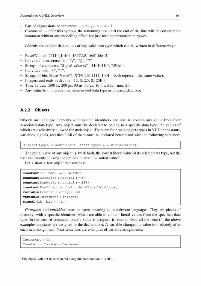
Signals are the most important objects in VHDL, and they are used to describe connections

between different components and processes in order to establish the data flow between resources that

model the related hardware.

Signals must be able to reflect their value evolution across time by continuously collecting current

and further values as shown in the next code box examples. For a “Signal” object, in comparison with

“Constants and Variables”, a more complex data structure is required, as we need to store events,

which are pairs of “value (vi) � time (ti)” in chronological order (the related signal reaches the value

vi at time ti). Such a data structure is called a Driver, as shown in Fig. A.1 which reflects the Y signal

waveform assignment below:

Reset <¼ ‘1’; -- Assigns value ‘1’ to signal Reset.

-- Next sentence changes Clock signal 10ns later.

Clock <¼ not Clock after 10ns;

-- Next sentence projects on signal Y a waveform of

-- different values at different times.

Y <¼ ‘0’, ‘1’ after 10 ns, ‘0’ after 15 ns, ‘1’ after 20 ns, ‘0’ after 28 ns, ‘1’ after

40 ns, ‘0’ after 50 ns;

Wewill come back to signal driver management for event-driven VHDL simulation flow and cycle.

Comment A.1

Observe that while constant and variable assignments use the symbol “:¼”, the symbol used for signal

assignments is “<¼”.

A.2.3 Data Types

VHDL is a strongly typed language: any object must belong to a specific previously defined data type

and can only be combined with expressions or objects of such data type. For this reason, conversion

functions among data types are usual in VHDL.

A data type defines a set of fixed and static values: the literals of such data type. Those are

therefore the only ones that the objects of such a data type can contain.

There are some basic data types already predefined in VHDL, but new user-defined data types and

subtypes are allowed. This provides a powerful capability for reaching higher abstraction levels in

VHDL descriptions. In this appendix, just a subset of predefined (integer, Boolean, bit, character,

bit_vector, string, real, time) and a few user-defined data types will be used. Most of the data types are

defined in “Packages” to allow their easy usage in any VHDL code. VHDL intrinsic data types are

declared in the “Standard Package” shown in the next code box with different data types: enumerated

(Boolean, bit, character, severity_level), ranged (integer, real, time), un-ranged arrays (string,

bit_vector), or subtypes (natural, positive):

Y

0 10 20 30 40 50 60 ns

00

10 15 20 28 40 501 0 1 0 1 0

Ydriver

tivi

Currentvalue

Futurevalues

Fig. A.1 Waveform

assigned to signal Y and its

related Driver


Package standard is

type boolean is (false, true);

type bit is (‘0’, ‘1’);

type character is (NUL, SOH, STX,. . ., “, ‘!’, ‘”’, ‘#’, ‘$’

,. . ., ‘0’, ‘1’, ‘2’, ‘3’, ‘4’, ‘5’, ‘6’, ‘7’,‘8’,‘9’,. . .

,. . ., ‘A’, ‘B’, ‘C’, ‘D’, ‘E’, ‘F’ ,. . ., ‘a’, ‘b’, ‘c’,. . .);

type severity_level is (note, warning, error, failure);

-- Implementation dependent definitions

type integer is range -(2**31-1) to (2**31-1);

type real is range -1.0e38 to 1.0e38;

type time is range 0 to 1e20

units fs; ps¼1000fs; ns¼1000ps; us¼1000ns; ms¼1000us;

sec¼1000ms; min¼60sec; hr¼60min;

end units time;

. . ./. . .

function NOW return TIME;

subtype natural is integer range 0 to integer’high;

subtype positive is integer range 1 to integer’high;

’high is an attribute of data-types and refers to the highest literal value of related data-types (integer in this case)

type string is array (positive range <>) of character;

type bit_vector is array (natural range <>) of bit;

. . ./. . .

End standard;

A.2.4 Operators

Operators are specific reserved words or symbols which identify different operations that can be

performed with objects and literals from different data types. Some of them are intrinsic to the

language (e.g., adding integers or reals) while others are defined in specific packages (e.g., adding

bit_vectors or signed bit strings).

Operators are defined by their symbols or specific words and their operand profiles (number, order,

and data type of each one); thus the same operator symbol or name can support multiple definitions by

different profiles (overloaded operators). Operators can only be used with their specific profile, not

with every data type.

A.2.5 VHDL Structure: Design Units

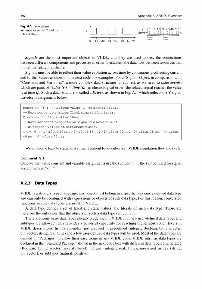
VHDL code is structured in different design units: entity, architecture, package (declaration and

body), and configuration.2 A typical single VHDL module is based on two parts or design units: one

simply defines the connections between this module and other external modules, while the other part

describes the behavior of the module. As shown in Fig. A.2 those two parts are the design units entity

and architecture.

2 Configuration design unit will be defined, but is not used in this text.


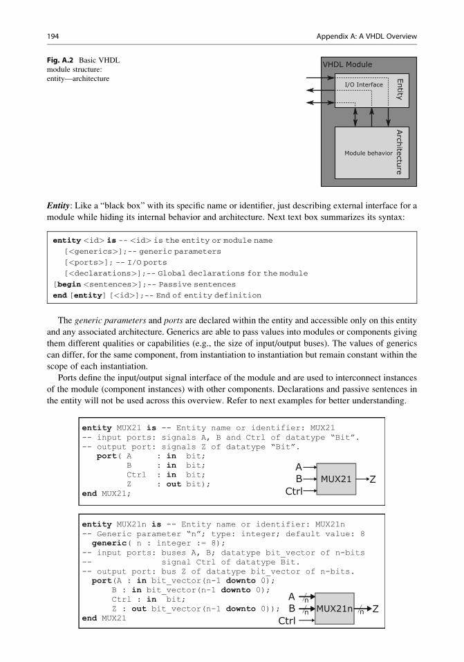
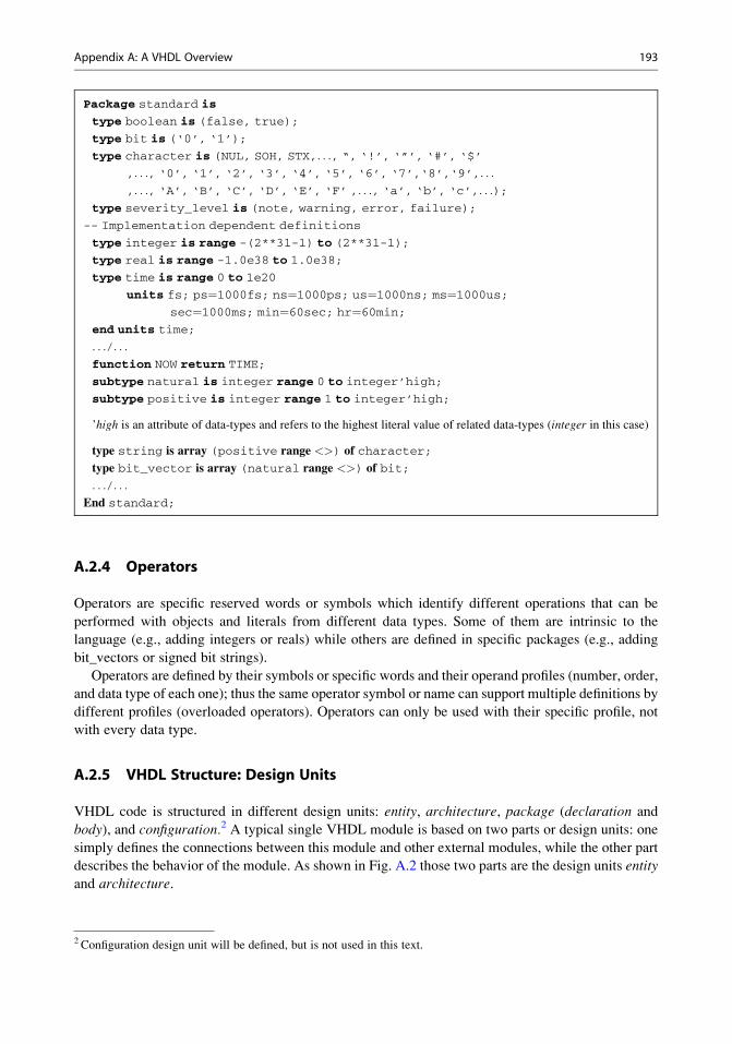
Entity: Like a “black box” with its specific name or identifier, just describing external interface for a

module while hiding its internal behavior and architecture. Next text box summarizes its syntax:

entity <id> is -- <id> is the entity or module name

[<generics>];-- generic parameters

[<ports>]; -- I/O ports

[<declarations>];-- Global declarations for the module

[begin <sentences>];-- Passive sentences

end [entity] [<id>];-- End of entity definition

The generic parameters and ports are declared within the entity and accessible only on this entity

and any associated architecture. Generics are able to pass values into modules or components giving

them different qualities or capabilities (e.g., the size of input/output buses). The values of generics

can differ, for the same component, from instantiation to instantiation but remain constant within the

scope of each instantiation.

Ports define the input/output signal interface of the module and are used to interconnect instances

of the module (component instances) with other components. Declarations and passive sentences in

the entity will not be used across this overview. Refer to next examples for better understanding.

entity MUX21 is -- Entity name or identifier: MUX21-- input ports: signals A, B and Ctrl of datatype “Bit”.-- output port: signals Z of datatype “Bit”.

port( A : in bit;B : in bit;Ctrl : in bit;Z : out bit);

end MUX21;

MUX21AB

CtrlZ

entity MUX21n is -- Entity name or identifier: MUX21n-- Generic parameter “n”; type: integer; default value: 8generic( n : integer := 8);

-- input ports: buses A, B; datatype bit_vector of n-bits-- signal Ctrl of datatype Bit.-- output port: bus Z of datatype bit_vector of n-bits.port(A : in bit_vector(n-1 downto 0);

B : in bit_vector(n-1 downto 0);Ctrl : in bit;Z : out bit_vector(n-1 downto 0));

end MUX21MUX21n Zn

AB

Ctrl

n

n

VHDL ModuleEntity

I/O Interface

Arch

itecture

Module behavior

Fig. A.2 Basic VHDL

module structure:

entity—architecture


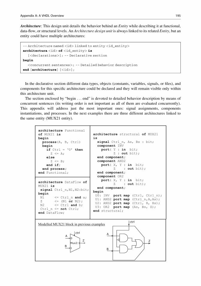
Architecture: This design unit details the behavior behind an Entity while describing it at functional,data-flow, or structural levels. An Architecture design unit is always linked to its related Entity, but an

entity could have multiple architectures:

-- Architecture named <id> linked to entity <id_entity>

architectura <id> of <id_entity> is

[<declarations>]; -- Declarative section

begin

<concurrent sentences>; -- Detailed behavior description

end [architecture] [<id>];

In the declarative section different data types, objects (constants, variables, signals, or files), and

components for this specific architecture could be declared and they will remain visible only within

this architecture unit.

The section enclosed by “begin . . . end” is devoted to detailed behavior description by means of

concurrent sentences (its writing order is not important as all of them are evaluated concurrently).

This appendix will address just the most important ones: signal assignments, components

instantiations, and processes. In the next examples there are three different architectures linked to

the same entity (MUX21 entity).

architecture Functional of MUX21 isbeginprocess(A, B, Ctrl)beginif Ctrl = ‘0’ thenZ <= A;

elseZ <= B;

end if;end process;

end Functional;

architecture DataFlow ofMUX21 issignal Ctrl_n,N1,N2:bit;beginN1 <= Ctrl_n and a;Z <= (N1 or N2);N2 <= Ctrl and b;Ctrl_n <= not Ctrl;end DataFlow;

architecture structural of MUX21 issignal Ctrl_n, As, Bs : bit;component INVport( Y : in bit;

Z : out bit);end component;component AND2port( X, Y : in bit;

Z : out bit);end component;component OR2port( X, Y : in bit;

Z : out bit);end component;

beginU0: INV port map (Ctrl, Ctrl_n);U1: AND2 port map (Ctrl_n,A,As);U2: AND2 port map (Ctrl, B, Bs);U3: OR2 port map (As, Bs, Z);end structural;

Modelled MUX21 block in previous examples

ctrl

Mux2:1

A

B

Z0

1

A

B

Z

ctrl


Comment A.2

In any of the three previous architectures, if they are linked to a MUX21n entity instead of MUX21,

the primary signals A, B, and Z will become n-bit buses.

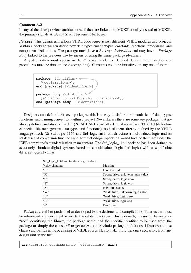
Package: This design unit allows VHDL code reuse across different VHDL modules and projects.

Within a package we can define new data types and subtypes, constants, functions, procedures, and

component declarations. The package must have a Package declaration and may have a PackageBody linked to the previous one by means of using the same package identifier.

Any declaration must appear in the Package, while the detailed definitions of functions or

procedures must be done in the Package Body. Constants could be initialized in any one of them.

package <identifier>[<declarations>];

end [package] [<identifier>]

package body <identifier>[<Assignments and Detailed definitions>];

end [package body] [<identifier>]

Designers can define their own packages; this is a way to define the boundaries of data types,

functions, and naming convention within a project. Nevertheless there are some key packages that are

already defined and standardized: (1) STANDARD (partially defined above) and TEXTIO (definition

of needed file management data types and functions), both of them already defined by the VHDL

language itself; (2) Std_logic_1164 and Std_logic_arith which define a multivalued logic and its

related set of conversion functions and arithmetic-logic operations—and both of them are under the

IEEE committee’s standardization management. The Std_logic_1164 package has been defined to

accurately simulate digital systems based on a multivalued logic (std_logic) with a set of nine

different logical values.

Std_logic_1164 multivalued logic values

Value character Meaning

“U” Uninitialized

“X” Strong drive, unknown logic value

“0” Strong drive, logic zero

“1” Strong drive, logic one

“Z” High impedance

“W” Weak drive, unknown logic value

“L” Weak drive, logic zero

“H” Weak drive, logic one

“-“ Don’t care

Packages are either predefined or developed by the designer and compiled into libraries that must

be referenced in order to get access to the related packages. This is done by means of the sentence

“use” identifying the library, the package name, and the specific identifier to be used from the

package or simply the clause all to get access to the whole package definitions. Libraries and use

clauses are written at the beginning of VHDL source files to make those packages accessible from any

design unit in the file:

use <library>.<package name>.[<identifier> | all];


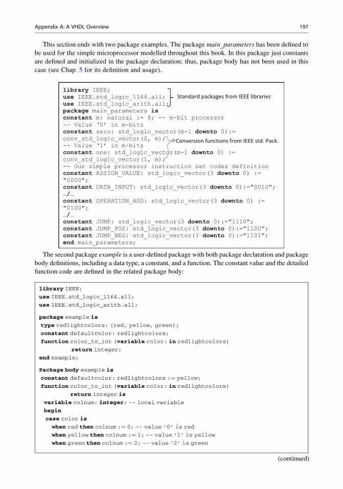
This section ends with two package examples. The package main_parameters has been defined to

be used for the simple microprocessor modelled throughout this book. In this package just constants

are defined and initialized in the package declaration; thus, package body has not been used in this

case (see Chap. 5 for its definition and usage).

library IEEE;use IEEE.std_logic_1164.all;use IEEE.std_logic_arith.all;package main_parameters isconstant m: natural := 8; -- m-bit processor-- Value ‘0’ in m-bitsconstant zero: std_logic_vector(m-1 downto 0):= conv_std_logic_vector(0, m);-- Value ‘1’ in m-bitsconstant one: std_logic_vector(m-1 downto 0) := conv_std_logic_vector(1, m);-- Our simple processor instruction set codes definitionconstant ASSIGN_VALUE: std_logic_vector(3 downto 0) :="0000";constant DATA_INPUT: std_logic_vector(3 downto 0):="0010";…/…constant OPERATION_ADD: std_logic_vector(3 downto 0) :="0100";…/…constant JUMP: std_logic_vector(3 downto 0):="1110";constant JUMP_POS: std_logic_vector(3 downto 0):="1100";constant JUMP_NEG: std_logic_vector(3 downto 0):="1101";end main_parameters;

Standard packages from IEEE libraries

Conversion functions from IEEE std. Pack.

o

C

The second package example is a user-defined package with both package declaration and package

body definitions, including a data type, a constant, and a function. The constant value and the detailed

function code are defined in the related package body:

library IEEE;

use IEEE.std_logic_1164.all;

use IEEE.std_logic_arith.all;

package example is

type redlightcolors: (red, yellow, green);

constant defaultcolor: redlightcolors;

function color_to_int (variable color: in redlightcolors)

return integer;

end example;

Package body example is

constant defaultcolor: redlightcolors :¼ yellow;

function color_to_int (variable color: in redlightcolors)

return integer is

variable colnum: integer; -- local variable

begin

case color is

when red then colnum :¼ 0; -- value ‘0’ is red

when yellow then colnum :¼ 1; -- value ‘1’ is yellow

when green then colnum :¼ 2; -- value ‘2’ is green

(continued)


http://dx.doi.org/10.1007/978-3-319-41198-9_5

end case;

return colnum;-- returned value

end;

end example;

The Configuration declaration design unit specifies different bounds: architectures to entities or an

entity-architecture to a component. These bound definitions are used in further simulation and

synthesis steps.

If there are multiple architectures for one entity, the configuration selects which architecture must

be bound to the entity. This way the designer can evaluate different architectures through simulation

and synthesis processes just changing the configuration unit.

For architectures using components, the configuration identifies a specific entity-architecture to be

bound to a specific component or component instantiation. Entity-architecture assigned to

components can be exchanged if they are port compatible with the component definition. This allows

for a component-based architecture, the evaluation of different entity-architectures mapped into the

different components of such architecture.

Configuration declarations are always optional and in their absence the VHDL specifies a set of

rules for a default configuration. As an example, in the case of multiple architectures for an entity, the

last compiled architecture will be bound to the entity for simulation and synthesis purposes by default.

As this design unit is not used in this book, we will not consider it in more depth.

A.3 Concurrent and Sequential Language for Hardware Modelling

Hardware behavior is inherently concurrent; thus, we need to model such a concurrency along time.

The VHDL language has resources to address both time and concurrency combined with sequential

behavior modelling.

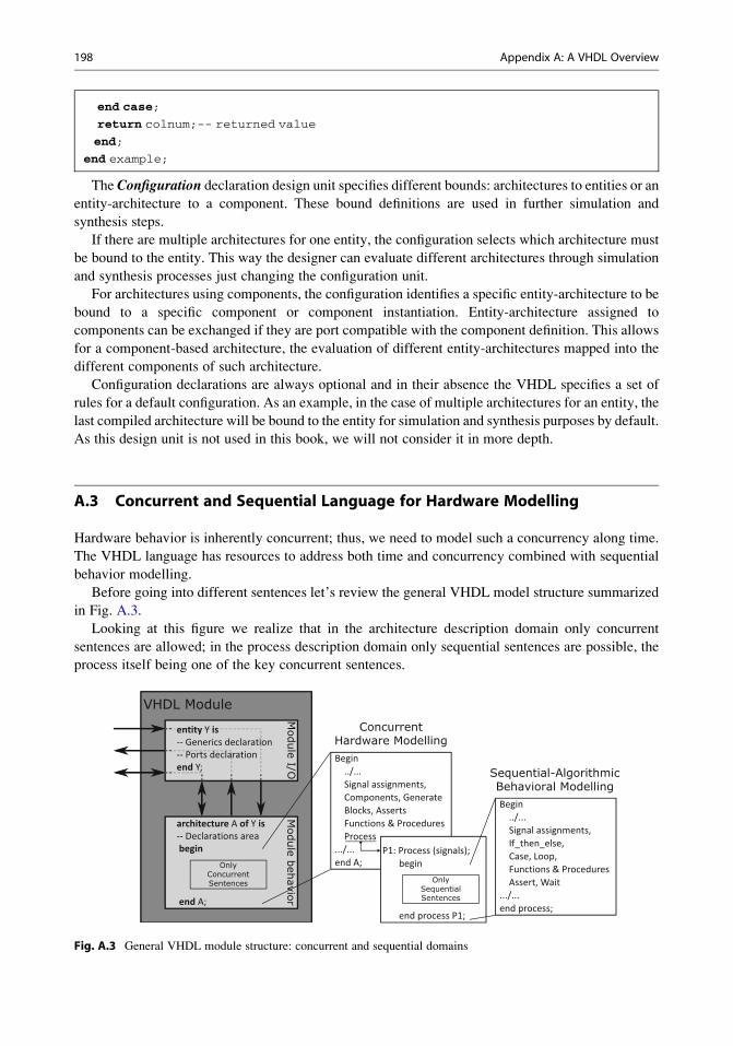
Before going into different sentences let’s review the general VHDL model structure summarized

in Fig. A.3.

Looking at this figure we realize that in the architecture description domain only concurrent

sentences are allowed; in the process description domain only sequential sentences are possible, the

process itself being one of the key concurrent sentences.

VHDL Module

Module I/O

entity Y is-- Generics declaration-- Ports declarationend Y;

Module b

ehavio

r

architecture A of Y is-- Declarations area begin

end A;

OnlyConcurrentSentences

Begin ../... Signal assignments, Components, Generate Blocks, Asserts Functions & Procedures Process.../...end A;

P1: Process (signals); begin

end process P1;

OnlySequentialSentences

Begin ../... Signal assignments, If_then_else, Case, Loop, Functions & Procedures Assert, Wait.../...end process;

ConcurrentHardware Modelling

Sequential-AlgorithmicBehavioral Modelling

Fig. A.3 General VHDL module structure: concurrent and sequential domains


Concurrent sentences are evaluated simultaneously; thus the writing order is not at all relevant.

Instead, sequential sentences are evaluated as such, following the order in which they have been

written; in this case the order of sentences is important to determine the result.

Generally speaking, it can be said that when we use concurrent VHDL statements we are doing

concurrent hardware modelling, while when we use sequential statements we perform an algorithmic

behavioral modelling. In any case, both domains can be combined in VHDL for modelling, simula-

tion, and synthesis purposes.

Figure A.3 also identifies the main sentences, concurrent and sequential, that we will address in this

introduction to VHDL, the process being one of the most important concurrent sentences that links both

worldswithin VHDL. In fact, any concurrent sentence will be translated into its equivalent process before

addressing any simulation or synthesis steps, which are simply managing lots of concurrent processes.

A.3.1 Sequential Sentences

Sequential sentences can be written in Processes, Functions, and Procedures. Now we will review a

small but relevant selection of those sentences.

Variable assignment sentence has the same meaning and behavior as in software languages. The

variable changes to the new value immediately after the assignment. Below you can find the syntax

where the differentiating symbol is “:¼” and the final expression value must belong to the variable

data type:

Syntax: [label:] <variable name> :¼ <expression>;

Examples: Var :¼ ‘0’; C :¼ my_function(4,adrbus) + A;

Vector :¼ “00011100”; B :¼ my_function(3,databus)

string :¼ “Message is: ”; A :¼ B + C;

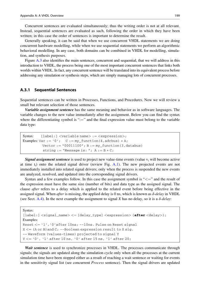
Signal assignment sentence is used to project new value-time events (value vi will become active

at time ti) onto the related signal driver (review Fig. A.1). The new projected events are not

immediately installed into related signal drivers; only when the process is suspended the new events

are analyzed, resolved, and updated into the corresponding signal drivers.

Syntax and a few examples follow. In this case the assignment symbol is “<¼” and the result of

the expression must have the same size (number of bits) and data type as the assigned signal. The

clause after refers to a delay which is applied to the related event before being effective in the

assigned signal. When after is missing, the applied delay is 0 ns, which is known as δ-delay in VHDL(see Sect. A.4). In the next example the assignment to signal X has no delay, so it is a δ-delay:

Syntax:

[label:] <signal_name> <¼ [delay_type] <expression> {after <delay>};

Examples:

Reset <¼ ‘1’,‘0’after 10ns; --10ns. Pulse on Reset signal

X <¼ (A or B)and C; --Boolean expression result to X sig.

-- Waveform (values-times) projected to signal Y

Y <¼ ‘0’, ‘1’ after 10 ns, ‘0’ after 15 ns, ‘1’ after 20;

Wait sentence is used to synchronize processes in VHDL. The processes communicate through

signals; the signals are updated along the simulation cycle only when all the processes at the current

simulation time have been stopped either as a result of reaching a wait sentence or waiting for events

in the sensitivity signal list (see concurrent Process sentence). Then the signal drivers are updated


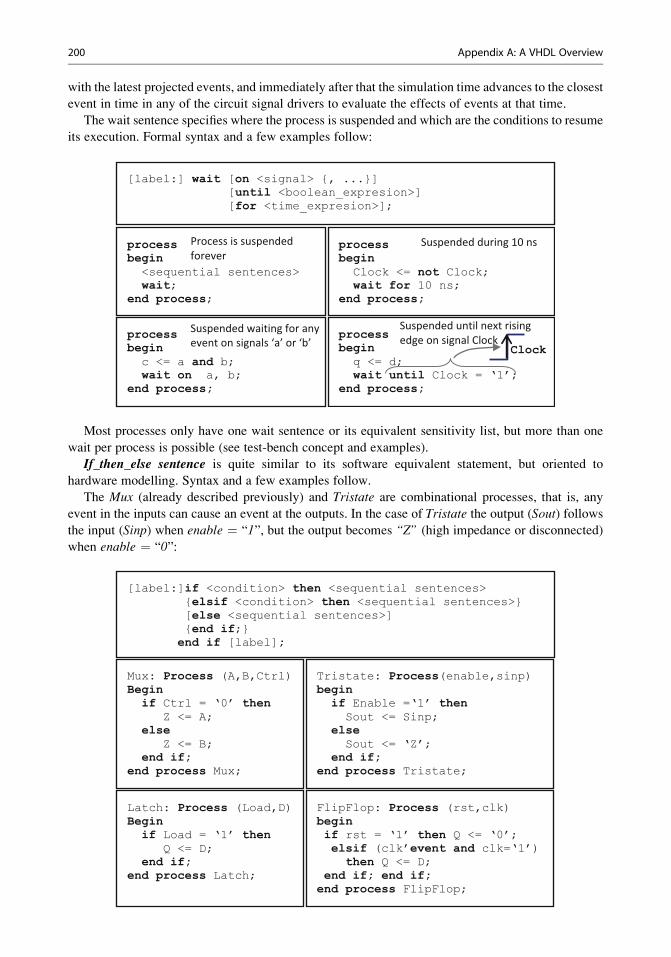
with the latest projected events, and immediately after that the simulation time advances to the closest

event in time in any of the circuit signal drivers to evaluate the effects of events at that time.

The wait sentence specifies where the process is suspended and which are the conditions to resume

its execution. Formal syntax and a few examples follow:

[label:] wait [on <signal> {, ...}][until <boolean_expresion>][for <time_expresion>];

processbegin

<sequential sentences>wait;

end process;

processbegin

Clock <= not Clock;wait for 10 ns;

end process;

processbeginc <= a and b;wait on a, b;

end process;

processbegin

q <= d;wait until Clock = ‘1’;

end process;

Process is suspended forever

Suspended waiting for anyevent on signals ‘a’ or ‘b’

Suspended during 10 ns

Suspended until next rising edge on signal Clock

Clock

Most processes only have one wait sentence or its equivalent sensitivity list, but more than one

wait per process is possible (see test-bench concept and examples).

If_then_else sentence is quite similar to its software equivalent statement, but oriented to

hardware modelling. Syntax and a few examples follow.

The Mux (already described previously) and Tristate are combinational processes, that is, any

event in the inputs can cause an event at the outputs. In the case of Tristate the output (Sout) follows

the input (Sinp) when enable ¼ “1”, but the output becomes “Z” (high impedance or disconnected)

when enable ¼ “0”:

[label:]if <condition> then <sequential sentences>{elsif <condition> then <sequential sentences>}[else <sequential sentences>]{end if;}

end if [label];

Mux: Process (A,B,Ctrl)Begin

if Ctrl = ‘0’ thenZ <= A;

elseZ <= B;

end if;end process Mux;

Tristate: Process(enable,sinp)begin

if Enable =‘1’ thenSout <= Sinp;

elseSout <= ‘Z’;

end if;end process Tristate;

Latch: Process (Load,D)Beginif Load = ‘1’ then

Q <= D;end if;

end process Latch;

FlipFlop: Process (rst,clk)beginif rst = ‘1’ then Q <= ‘0’;elsif (clk’event and clk=‘1’)

then Q <= D;end if; end if;

end process FlipFlop;


The Latch and FlipFlop processes model devices able to store binary information, and both of

them contain one incompletely specified if-then-else sentence: in the latch model there is no else

clause and in the flip-flop model there is no inner else clause. In both cases when the clause elsebecomes true, no action is specified on the output (Q); therefore such signal keeps the previous value;

this requires a memory element. The above codes model such kind of memory devices.

In the above latch case, Q will accept any new value on D while Load ¼ “1”, but Q will keep the

latest stored value when Load ¼ “0”.

In the other example, flip-flop reacts only to events in signals rst and clk. At any time, if rst ¼ “1”

then Q ¼ “0”.When rst ¼ “0” (not active) then clk takes the control, and at the rising edge of this clksignal (condition clk’event3 and clk ¼ “1”), then, and only then, the Q output signal takes the value

from D at this precise instant of time and stores this value till next rst ¼ “1” or rising edge in clk.

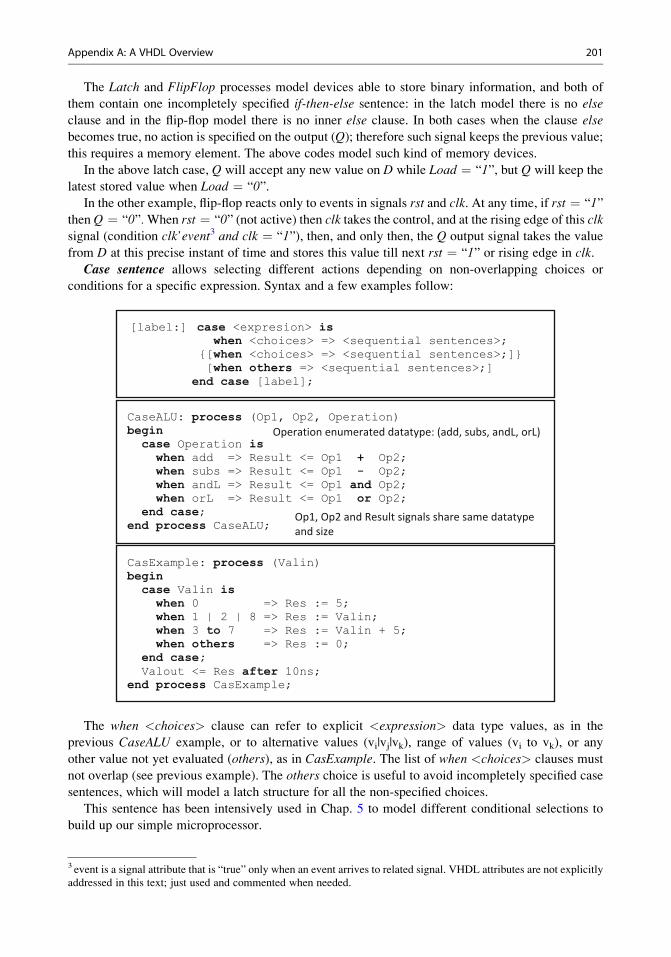
Case sentence allows selecting different actions depending on non-overlapping choices or

conditions for a specific expression. Syntax and a few examples follow:

[label:] case <expresion> iswhen <choices> => <sequential sentences>;

{[when <choices> => <sequential sentences>;]}[when others => <sequential sentences>;]

end case [label];

CaseALU: process (Op1, Op2, Operation)begin

case Operation iswhen add => Result <= Op1 + Op2;when subs => Result <= Op1 - Op2;when andL => Result <= Op1 and Op2;when orL => Result <= Op1 or Op2;

end case;end process CaseALU;

CasExample: process (Valin)begincase Valin is

when 0 => Res := 5;when 1 | 2 | 8 => Res := Valin;when 3 to 7 => Res := Valin + 5;when others => Res := 0;

end case;Valout <= Res after 10ns;

end process CasExample;

Operation enumerated datatype: (add, subs, andL, orL)

Op1, Op2 and Result signals share same datatype and size

The when <choices> clause can refer to explicit <expression> data type values, as in the

previous CaseALU example, or to alternative values (vi|vj|vk), range of values (vi to vk), or any

other value not yet evaluated (others), as in CasExample. The list of when <choices> clauses must

not overlap (see previous example). The others choice is useful to avoid incompletely specified case

sentences, which will model a latch structure for all the non-specified choices.

This sentence has been intensively used in Chap. 5 to model different conditional selections to

build up our simple microprocessor.

3 event is a signal attribute that is “true” only when an event arrives to related signal. VHDL attributes are not explicitly

addressed in this text; just used and commented when needed.


http://dx.doi.org/10.1007/978-3-319-41198-9_5

Comment A.3

Any conditional assignment or sentence where not all the condition possibilities have been addressed,

explicitly or with a default value (using clause “others” or assigning a value to related signal just

before the conditional assignment or sentence), will infer a latch structure.

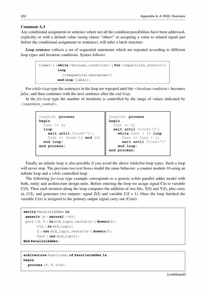
Loop sentence collects a set of sequential statements which are repeated according to different

loop types and iteration conditions. Syntax follows:

[label:] [while <boolean_condition> | for <repetition_control>]

loop

{<sequential sentences>}

end loop [label];

For while-loop type the sentences in the loop are repeated until the<boolean condition> becomes

false, and then continues with the next sentence after the end loop.In the for-loop type the number of iterations is controlled by the range of values indicated by

<repetition_control>.

Count16: processbegin

Cont <= 0;loopwait until Clock=‘1’;Cont <= (Cont+1) mod 16;

end loop;end process;

Count16: processbeginCont <= 0;wait until Clock=‘1’;

while Cont < 15 loopCont <= Cont + 1;wait until Clock=‘1’


Finally an infinite loop is also possible if you avoid the above while/for-loop types. Such a loop

will never stop. The previous two text boxes model the same behavior: a counter modulo 16 using an

infinite loop and a while controlled loop.

The following for-loop type example corresponds to a generic n-bits parallel adder model with

both, entity and architecture design units. Before entering the loop we assign signal Cin to variable

C(0). Then each iteration along the loop computes the addition of two bits, X(I) and Y(I), plus carry

in, C(I), and generates two outputs: signal Z(I) and variable C(I + 1). Once the loop finished the

variable C(n) is assigned to the primary output signal carry out (Cout):

entity ParallelAdder is

generic (n : natural :¼4);

port ( X, Y : in std_logic_vector(n-1 downto 0);

Cin : in std_logic;

Z : out std_logic_vector(n-1 downto 0);

Cout : out std_logic);

End ParallelAdder;

achitecture Functional of ParallelAdder is

begin

process (X, Y, Cin);

(continued)


variable C : std_logic_vector(n downto 0);

variable tmp : std_logic;

variable I : integer;

begin

C(0) :¼ Cin;

for I in 0 to n-1 loop

tmp :¼ X(I) xor Y(I);

Z(I) <¼ tmp xor C(I);

C(I+1) :¼ (tmp and C(I)) or (X(I) and Y(I));

end loop;

Cout <¼ C(n);

end process;

end Functional;

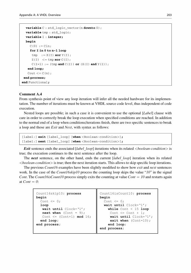
Comment A.4

From synthesis point of view any loop iteration will infer all the needed hardware for its implemen-

tation. The number of iterations must be known at VHDL source code level, thus independent of code

execution.

Nested loops are possible; in such a case it is convenient to use the optional [Label] clause with

care in order to correctly break the loop execution when specified conditions are reached. In addition

to the normal end of a loop when conditions/iterations finish, there are two specific sentences to break

a loop and those are Exit and Next, with syntax as follows:

[label:] exit [label_loop] [when <Boolean-condition>];

[label:] next [label_loop] [when <Boolean-condition>];

Exit sentence ends the associated [label_loop] iterations when its related <boolean-condition> is

true; the execution continues to the next sentence after the loop.

The next sentence, on the other hand, ends the current [label_loop] iteration when its related

<boolean-condition> is true; then the next iteration starts. This allows to skip specific loop iterations.

The previous Count16 examples have been slightly modified to show how exit and next sentences

work. In the case of the Count16skip10 process the counting loop skips the value “10” in the signal

Cont. The Count16isCount10 process simply exits the counting at value Cont ¼ 10 and restarts again

at Cont ¼ 0:

Count16skip10: processbegin

Cont <= 0;loopwait until Clock=‘1’;next when (Cont = 9);Cont <= (Cont+1) mod 16;


Count16isCount10: processbegin

Cont <= 0;wait until Clock=‘1’;while Cont < 15 loopCont <= Cont + 1;wait until Clock=‘1’;exit when (Cont=10);end loop;

end process;


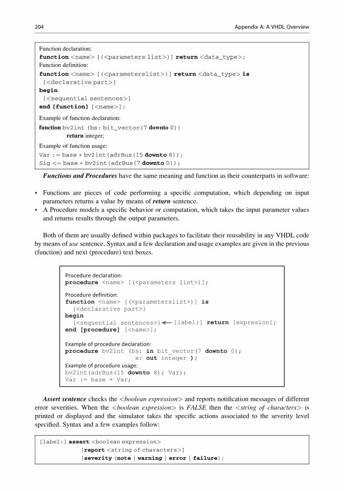
Function declaration:

function <name> [(<parameters list>)] return <data_type>;

Function definition:

function <name> [(<parameterslist>)] return <data_type> is

{<declarative part>}

begin

{<sequential sentences>}

end [function] [<name>];

Example of function declaration:

function bv2int (bs: bit_vector(7 downto 0))

return integer;

Example of function usage:

Var :¼ base + bv2int(adrBus(15 downto 8));

Sig <¼ base + bv2int(adrBus(7 downto 0));

Functions and Procedures have the same meaning and function as their counterparts in software:

• Functions are pieces of code performing a specific computation, which depending on input

parameters returns a value by means of return sentence.

• A Procedure models a specific behavior or computation, which takes the input parameter values

and returns results through the output parameters.

Both of them are usually defined within packages to facilitate their reusability in any VHDL code

by means of use sentence. Syntax and a few declaration and usage examples are given in the previous

(function) and next (procedure) text boxes.

Procedure declaration:procedure <name> [(<parameters list>)];

Procedure definition:function <name> [(<parameterslist>)] is

{<declarative part>}begin{<sequential sentences>}

end [procedure] [<name>];

Example of procedure declaration:procedure bv2int (bs: in bit_vector(7 downto 0);

x: out integer );Example of procedure usage:bv2int(adrBus(15 downto 8); Var); Var := base + Var;

[label:] return [expresion];

Assert sentence checks the <boolean expression> and reports notification messages of different

error severities. When the <boolean expression> is FALSE then the <string of characters> is

printed or displayed and the simulator takes the specific actions associated to the severity level

specified. Syntax and a few examples follow:

[label:] assert <boolean expression>

[report <string of characters>]

[severity (note | warning | error | failure);


assert not(addr < X"00001000" or addr > X"0000FFFF“)

report “Address in range" severity note;

assert (J /¼ C) report "J ¼ C" severity note;

The sentence report has been included in VHDL for notification purposes—not to check any

Boolean expression—with the following syntax and related example:

[label:] [report < string of characters >]

[severity (note | warning | error | failure);

Example:

report “Check point 13”; -- is fully equivalent to . . .

assert FALSE “Check point 13” severity note;

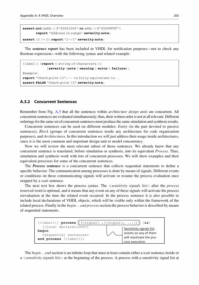
A.3.2 Concurrent Sentences

Remember from Fig. A.3 that all the sentences within architecture design units are concurrent. All

concurrent sentences are evaluated simultaneously; thus, their written order is not at all relevant. Different

orderings for the same set of concurrent sentencesmust produce the same simulation and synthesis results.

Concurrent sentences can be used on different modules: Entity (in the part devoted to passive

sentences), Block (groups of concurrent sentences inside any architecture for code organization

purposes), and Architectures. In this introduction we will just address their usage inside architectures,

since it is the most common and important design unit to model concurrency.

Now we will review the most relevant subset of those sentences. We already know that any

concurrent sentence is translated, before simulation or synthesis, into its equivalent Process. Thus,

simulation and synthesis work with lots of concurrent processes. We will show examples and their

equivalent processes for some of the concurrent sentences.

The Process sentence is a concurrent sentence that collects sequential statements to define a

specific behavior. The communication among processes is done by means of signals. Different events

or conditions on these communicating signals will activate or resume the process evaluation once

stopped by a wait sentence.

The next text box shows the process syntax. The <sensitivity signals list> after the process

reserved word is optional, and it means that any event on any of these signals will activate the process

reevaluation at the time the related event occurred. In the process sentence it is also possible to

include local declarations of VHDL objects, which will be visible only within the framework of the

related process. Finally in the begin. . .end process section the process behavior is described by means

of sequential statements.

[<label>:] process [(<signal> ,{<signal>, ...})] [is][<local declarations>]

begin<sequential sentences>

end process [<label>];

Sensitivity signals list: events on any of them will reactivate the pro-cess execution

The begin. . .end section is an infinite loop that must at least contain either a wait sentence inside or

a <sensitivity signals list> at the beginning of the process. A process with a sensitivity signal list at


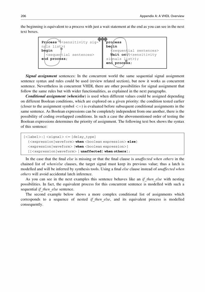
the beginning is equivalent to a process with just a wait statement at the end as you can see in the next

text boxes.

Process (<sensitivity sig-nals list>)begin

<sequential sentences>end process;

processbegin

<sequential sentences>Wait on (<sensitivity

signals list>);end process;

Signal assignment sentences: In the concurrent world the same sequential signal assignment

sentence syntax and rules could be used (review related section), but now it works as concurrent

sentence. Nevertheless in concurrent VHDL there are other possibilities for signal assignment that

follow the same rules but with wider functionalities, as explained in the next paragraphs.

Conditional assignment (when/else) is used when different values could be assigned depending

on different Boolean conditions, which are explored on a given priority: the condition tested earlier

(closer to the assignment symbol <¼) is evaluated before subsequent conditional assignments in the

same sentence. As Boolean expressions can be completely independent from one another, there is the

possibility of coding overlapped conditions. In such a case the abovementioned order of testing the

Boolean expressions determines the priority of assignment. The following text box shows the syntax

of this sentence:

[<label>:] <signal> <¼ [delay_type]

{<expression|waveform> when <boolean expression> else}

<expression|waveform> [when <boolean expression>]

[[<expression|waveform> | unaffected] when others];

In the case that the final else is missing or that the final clause is unaffected when others in the

chained list of when/else clauses, the target signal must keep its previous value; thus a latch is

modelled and will be inferred by synthesis tools. Using a final else clause instead of unaffected when

others will avoid accidental latch inference.

As you can see in the next examples this sentence behaves like an if_then_else with nesting

possibilities. In fact, the equivalent process for this concurrent sentence is modelled with such a

sequential if_then_else sentence.

The second example below shows a more complex conditional list of assignments which

corresponds to a sequence of nested if_then_else, and its equivalent process is modelled

consequently.


Concurrent sentence:S <= A when Sel = ‘0’ else B;-- Sel is one bit signal

Concurrent sentence:S <= E1 when Sel2 = “00” else

E2 when Sel2 = “11” elseunaffected when others;

-- Sel is two bits signal

Due to unaffected clause a latch will be inferred on signal S to keep its previous valuewhen Sel2 value is neither “00” nor “11”.

Equivalent process:process (Sel, A, B)beginif Sel = ‘0’ then

S <= A;else

S <= B;end if;

end process;

Equivalent process:process (Sel2, E1, E2)begin

if Sel2 = “00” thenS <= E1;

elsif Sel2 = “11” thenS <= E2;

elsenull;

end if;end process;

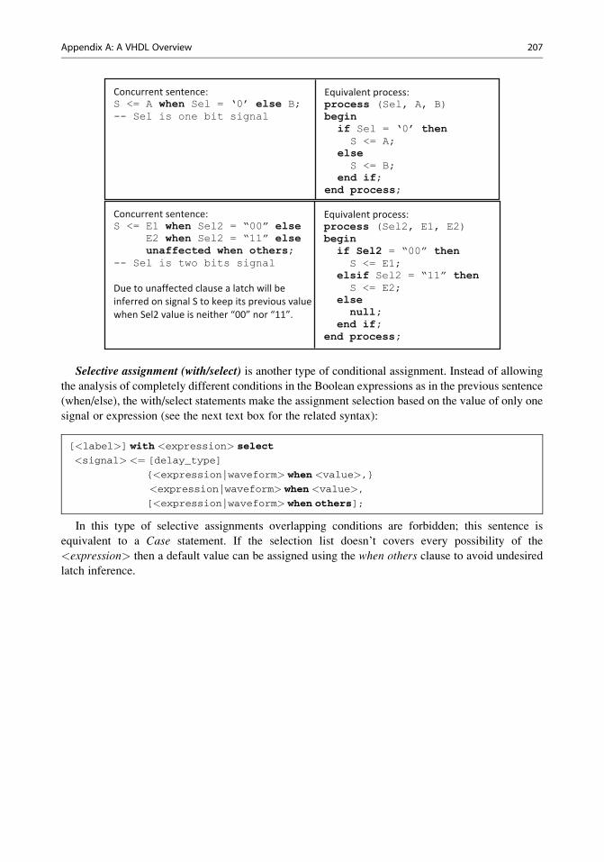
Selective assignment (with/select) is another type of conditional assignment. Instead of allowing

the analysis of completely different conditions in the Boolean expressions as in the previous sentence

(when/else), the with/select statements make the assignment selection based on the value of only one

signal or expression (see the next text box for the related syntax):

[<label>] with <expression> select

<signal> <¼ [delay_type]

{<expression|waveform> when <value>,}

<expression|waveform> when <value>,

[<expression|waveform> when others];

In this type of selective assignments overlapping conditions are forbidden; this sentence is

equivalent to a Case statement. If the selection list doesn’t covers every possibility of the

<expression> then a default value can be assigned using the when others clause to avoid undesired

latch inference.


The next example shows a simple usage of this concurrent selective assignment sentence and the

equivalent concurrent process, which is based on a sequential Case statement:

Concurrent sentence:with Operation selectResult <= Op1 + Op2 when add,

Op1 - Op2 when subs,Op1 and Op2 when andL,Op1 or Or2 when orL;

Equivalent process:process (Op1, Op2, Operation)begincase Operation is

when add => Result <= Op1 + Op2;when subs => Result <= Op1 - Op2;when andL => Result <= Op1 and Op2;when orL => Result <= Op1 or Op2;

end case;end process;

Operation enumerated datatype is: (add, subs, andL, orL).Op1, Op2 and Result signals share same datatype and size.

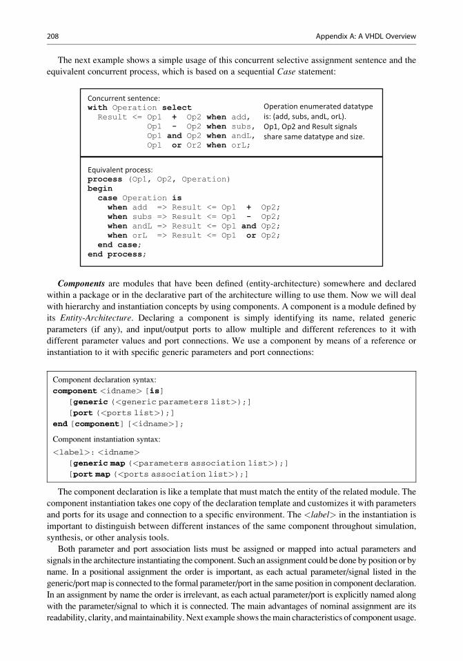
Components are modules that have been defined (entity-architecture) somewhere and declared

within a package or in the declarative part of the architecture willing to use them. Now we will deal

with hierarchy and instantiation concepts by using components. A component is a module defined by

its Entity-Architecture. Declaring a component is simply identifying its name, related generic

parameters (if any), and input/output ports to allow multiple and different references to it with

different parameter values and port connections. We use a component by means of a reference or

instantiation to it with specific generic parameters and port connections:

Component declaration syntax:

component <idname> [is]

[generic (<generic parameters list>);]

[port (<ports list>);]

end [component] [<idname>];

Component instantiation syntax:

<label>: <idname>

[generic map (<parameters association list>);]

[port map (<ports association list>);]

The component declaration is like a template that must match the entity of the related module. The

component instantiation takes one copy of the declaration template and customizes it with parameters

and ports for its usage and connection to a specific environment. The <label> in the instantiation is

important to distinguish between different instances of the same component throughout simulation,

synthesis, or other analysis tools.

Both parameter and port association lists must be assigned or mapped into actual parameters and

signals in the architecture instantiating the component. Such an assignment could be done by position or by

name. In a positional assignment the order is important, as each actual parameter/signal listed in the

generic/port map is connected to the formal parameter/port in the same position in component declaration.

In an assignment by name the order is irrelevant, as each actual parameter/port is explicitly named along

with the parameter/signal to which it is connected. The main advantages of nominal assignment are its

readability, clarity, andmaintainability. Next example shows themain characteristics of component usage.


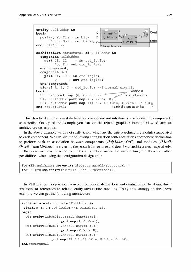
entity FullAdder isbeginport(X, Y, Cin : in bit;

Cout, Sum : out bit);end FullAdder;

architecture structural of FullAdder iscomponent HalfAdder

port(I1, I2 : in std_logic;Co, S : out std_logic);

end component;component OrGport(I1, I2 : in std_logic;

O : out std_logic);end component;signal A, B, C : std_logic; --Internal signals

beginU3: OrG port map (A, C, Cout);U1: HalfAdder port map (X, Y, A, B);U2: HalfAdder port map (I1=>B, I2=>Cin, S=>Sum, Co=>C);

end structural;

Positional association lists

Nominal association list

This structural architecture style based on component instantiation is like connecting components

as a netlist. On top of the example you can see the related graphic schematic view of such an

architecture description.

In the above example we do not really know which are the entity-architecture modules associated

to each component. We can add the following configuration sentences after a component declaration

to perform such an association between components {HalfAdder, OrG} and modules {HAcell,Orcell} from LibCells library using the so-called structural and functional architectures, respectively.

In this case we have done an explicit configuration inside the architecture, but there are other

possibilities when using the configuration design unit:

for all: HalfAdder use entity LibCells.HAcell(structural);

for U3: OrG use entity LibCells.Orcell(functional);

In VHDL it is also possible to avoid component declaration and configuration by doing direct

instances or references to related entity-architecture modules. Using this strategy in the above

example we can get the following architecture:

architecture structural of FullAdder is

signal A, B, C : std_logic; --Internal signals

begin

U3: entity LibCells.Orcell(functional)

port map (A, C, Cout);

U1: entity LibCells.HAcell(structural)

port map (X, Y, A, B);

U2: entity LibCells.HAcell(structural)

port map (I1¼>B, I2¼>Cin, S¼>Sum, Co¼>C);

end structural;


Generate sentence contains further concurrent statements that are to be replicated under con-

trolled criteria (conditions or repetitions). As you can see in the syntax, it looks similar to a for_loop

and indeed behaves like and serves a similar purpose, but in a concurrent code. In this sense all the

iterations within the generate loop will produce all the needed hardware; the number of iterations

must be known at VHDL source code level. Thus, they cannot depend on code execution:

<label>: {[for <range specification> | if <condition> ]}

generate

{<concurrent sentences>}

end generate;

The <label> is required to identify each specific generated structure. There are two forms for the

generate statement, conditional and repetitive (loop), and both can be combined. Any concurrent

statement is accepted within the body of generate; however the most common are component

instantiations.

Often the generate sentence is used in architectures working with generic parameters, as such

parameters are used to control the generate conditions (either form). This way a module can be

quickly adjusted to fit into different environments or applications (i.e., number of bits or operational

range of the module).

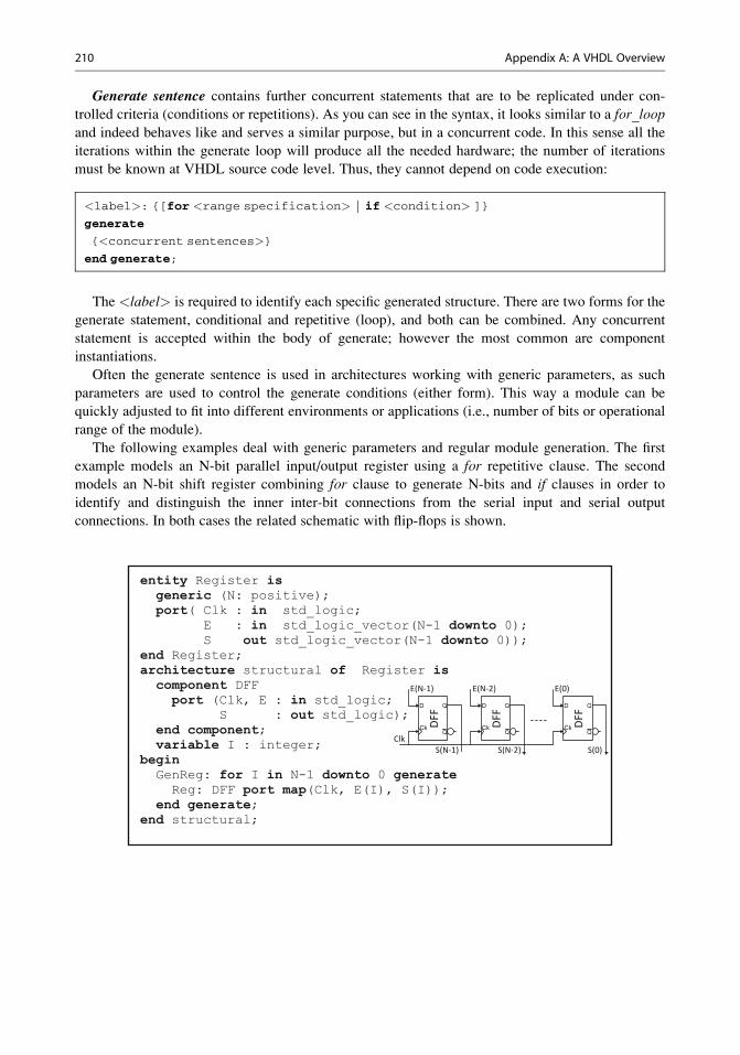
The following examples deal with generic parameters and regular module generation. The first

example models an N-bit parallel input/output register using a for repetitive clause. The second

models an N-bit shift register combining for clause to generate N-bits and if clauses in order to

identify and distinguish the inner inter-bit connections from the serial input and serial output

connections. In both cases the related schematic with flip-flops is shown.

entity Register isgeneric (N: positive);port( Clk : in std_logic;

E : in std_logic_vector(N-1 downto 0);S out std_logic_vector(N-1 downto 0));

end Register;architecture structural of Register is

component DFFport (Clk, E : in std_logic;

S : out std_logic);end component;variable I : integer;

beginGenReg: for I in N-1 downto 0 generateReg: DFF port map(Clk, E(I), S(I));

end generate;end structural;

QD

CkQ

DFF

E(N-1)

S(N-1)

QD

CkQ

DFF

E(N-2)

S(N-2)

QD

CkQ

DFF

E(0)

S(0)Clk


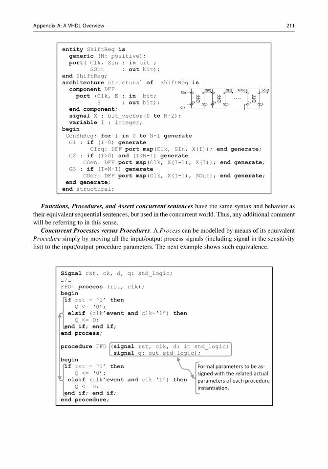
entity ShiftReg isgeneric (N: positive);port( Clk, SIn : in bit ;

SOut : out bit);end ShiftReg;architecture structural of ShiftReg is

component DFFport (Clk, E : in bit;

S : out bit);end component;signal X : bit_vector(0 to N-2);variable I : integer;

beginGenShReg: for I in 0 to N-1 generateG1 : if (I=0) generate

CIzq: DFF port map(Clk, SIn, X(I)); end generate;G2 : if (I>0) and (I<N-1) generate

CCen: DFF port map(Clk, X(I-1), X(I)); end generate;G3 : if (I=N-1) generate

CDer: DFF port map(Clk, X(I-1), SOut); end generate;end generate;

end structural;

QD

CkQ

DFF

X(0)Sin QD

CkQ

DFF

X(1)QD

CkQ

DFF

SoutX(N-1)

Clk

Functions, Procedures, and Assert concurrent sentences have the same syntax and behavior as

their equivalent sequential sentences, but used in the concurrent world. Thus, any additional comment

will be referring to in this sense.

Concurrent Processes versus Procedures. A Process can be modelled by means of its equivalent

Procedure simply by moving all the input/output process signals (including signal in the sensitivity

list) to the input/output procedure parameters. The next example shows such equivalence.

Signal rst, ck, d, q: std_logic;…/…FFD: process (rst, clk); beginif rst = ‘1’ then

Q <= ‘0’;elsif (clk’event and clk=‘1’) then

Q <= D;end if; end if;

end process;

procedure FFD (signal rst, clk, d: in std_logic;signal q: out std_logic);

beginif rst = ‘1’ then

Q <= ‘0’;elsif (clk’event and clk=‘1’) thenQ <= D;

end if; end if;end procedure;

Formal parameters to be as-signed with the related actual parameters of each procedure instantiation.


The Process is defined and used in the same place. For multiple uses you need to cut and paste it or

move it into a module (entity-architecture), to use it as a component to allow an easy reuse.

The Procedure is declared and defined within a package, and the clause use makes it accessible to

be instantiated with actual parameters assigned to formal parameters; thus, it is easily reusable. The

concurrent procedure call is also translated to its equivalent process before any simulation, synthesis,

or analysis steps.

Comment A.5

We have finished the introduction to VHDL language; now you will be able to read and understand

the examples of digital circuit models (combinational-sequential logic and finite-state machines)

already presented in previous chapters.

Combinational and sequential VHDL models related to processor blocks have been introduced in

Chap. 5 during the simple processor design. Finite-state machine definition and VHDL coding are

presented in Sect. 4.8, while different examples are shown in Sect. 4.9.

A.4 VHDL Simulation and Test-Benches

A.4.1 VHDL-Based Design Flow

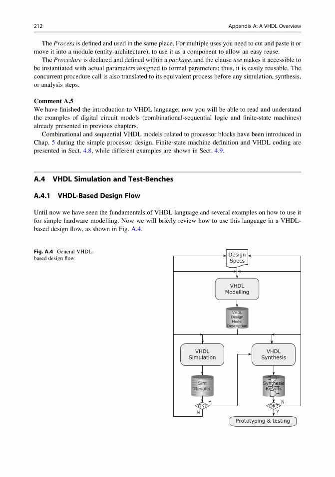
Until now we have seen the fundamentals of VHDL language and several examples on how to use it

for simple hardware modelling. Now we will briefly review how to use this language in a VHDL-

based design flow, as shown in Fig. A.4.

VHDLDesignModel

Description

DesignSpecs

VHDLModelling

VHDLSimulation

Y

N Y

N

VHDLSynthesis

OK? OK?

Prototyping & testing

SynthesisResults

Fig. A.4 General VHDL-

based design flow


http://dx.doi.org/10.1007/978-3-319-41198-9_5

http://dx.doi.org/10.1007/978-3-319-41198-9_4

http://dx.doi.org/10.1007/978-3-319-41198-9_4

Starting from design specifications, the first step is to develop a VHDLmodel for a target hardware

that fulfills the specifications for both functionality and performance. The VHDL model produced in

this initial modelling phase will be the starting point for further simulation and synthesis steps.

In order to ensure that the model fulfills the requested specifications we need to validate it by

means of several refinement iterations of modelling, simulation and analysis steps.

Once the quality of the model is assured by simulation we can address the next step: the hardware

design or synthesis to get the model materialized in the target technology. Once again, this phase may

require several improvement iterations.

Writing models with VHDL is the one and only way to learn the language. To do so we need to

verify that all models do what they are intended to do by means of test-bench-based simulations.

Modelling with VHDL has been addressed through small examples in this appendix and in other

larger examples throughout Chaps. 4, 5, and 6 of this book. Now we will address the basic concepts

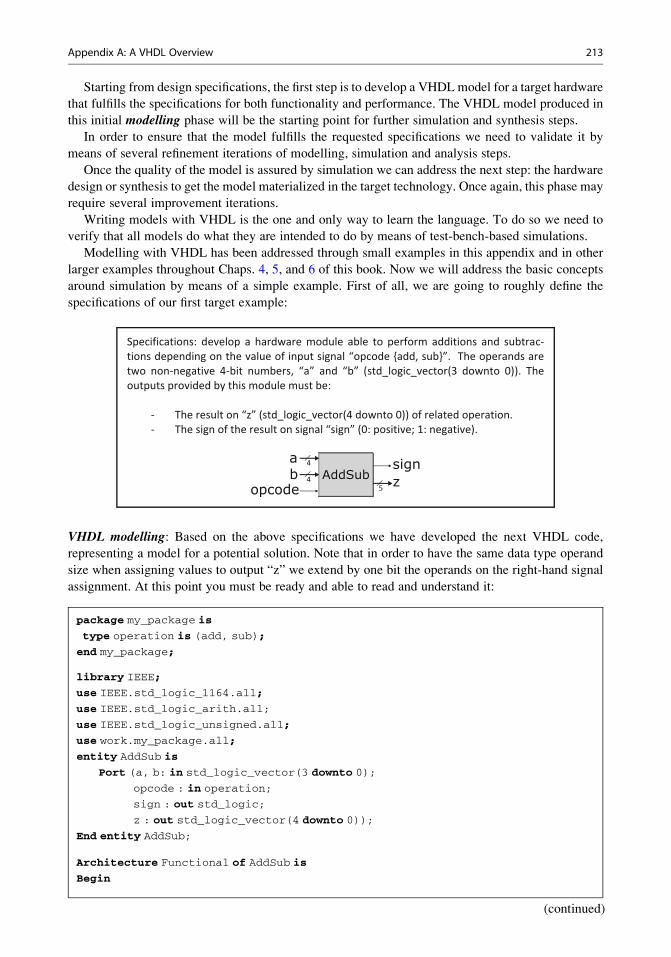
around simulation by means of a simple example. First of all, we are going to roughly define the

specifications of our first target example:

Specifications: develop a hardware module able to perform additions and subtrac-tions depending on the value of input signal “opcode {add, sub}”. The operands are two non-negative 4-bit numbers, “a” and “b” (std_logic_vector(3 downto 0)). The outputs provided by this module must be:

- The result on “z” (std_logic_vector(4 downto 0)) of related operation.- The sign of the result on signal “sign” (0: positive; 1: negative).

AddSubab

opcode zsign4

45

VHDL modelling: Based on the above specifications we have developed the next VHDL code,

representing a model for a potential solution. Note that in order to have the same data type operand

size when assigning values to output “z” we extend by one bit the operands on the right-hand signal

assignment. At this point you must be ready and able to read and understand it:

package my_package is

type operation is (add, sub);

end my_package;

library IEEE;

use IEEE.std_logic_1164.all;

use IEEE.std_logic_arith.all;

use IEEE.std_logic_unsigned.all;

use work.my_package.all;

entity AddSub is

Port (a, b: in std_logic_vector(3 downto 0);

opcode : in operation;

sign : out std_logic;

z : out std_logic_vector(4 downto 0));

End entity AddSub;

Architecture Functional of AddSub is

Begin

(continued)


http://dx.doi.org/10.1007/978-3-319-41198-9_4

http://dx.doi.org/10.1007/978-3-319-41198-9_5

http://dx.doi.org/10.1007/978-3-319-41198-9_6

Operation: process (a, b, opcode)

variable x, y : std_logic_vector(3 downto 0);

variable s : std_logic;

begin

if a >¼ b then x :¼ a; y :¼ b; s :¼ ‘0’;

else x :¼ b; y :¼ a; s :¼ ‘1’; end if;

case opcode is

when add then z <¼ (‘0’&x) + (‘0’&y); sign <¼ ‘0’;

when sub then z <¼ (‘0’&x) – (‘0’&y); sign <¼ s;

‐‐&: concatenation operation for bit or character strings

end case;

end process Operation;

End Architecture Functional;

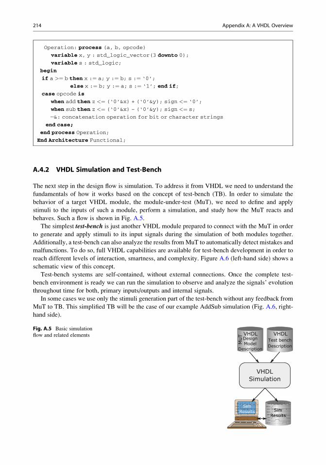
A.4.2 VHDL Simulation and Test-Bench

The next step in the design flow is simulation. To address it from VHDL we need to understand the

fundamentals of how it works based on the concept of test-bench (TB). In order to simulate the

behavior of a target VHDL module, the module-under-test (MuT), we need to define and apply

stimuli to the inputs of such a module, perform a simulation, and study how the MuT reacts and

behaves. Such a flow is shown in Fig. A.5.

The simplest test-bench is just another VHDL module prepared to connect with the MuT in order

to generate and apply stimuli to its input signals during the simulation of both modules together.

Additionally, a test-bench can also analyze the results fromMuT to automatically detect mistakes and

malfunctions. To do so, full VHDL capabilities are available for test-bench development in order to

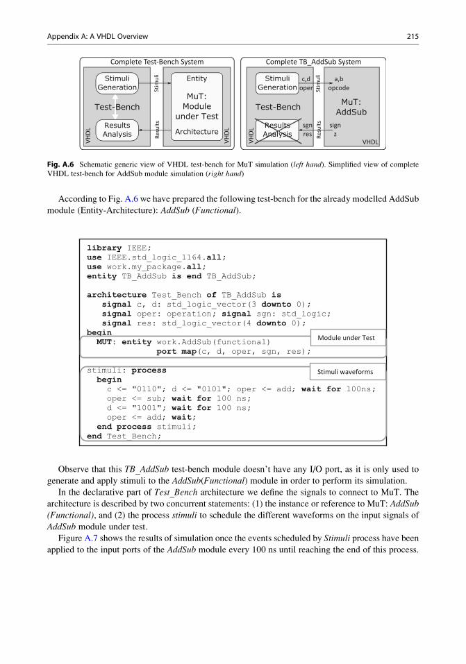
reach different levels of interaction, smartness, and complexity. Figure A.6 (left-hand side) shows a

schematic view of this concept.

Test-bench systems are self-contained, without external connections. Once the complete test-

bench environment is ready we can run the simulation to observe and analyze the signals’ evolution

throughout time for both, primary inputs/outputs and internal signals.

In some cases we use only the stimuli generation part of the test-bench without any feedback from

MuT to TB. This simplified TB will be the case of our example AddSub simulation (Fig. A.6, right-

hand side).

VHDLDesignModel

Description

VHDL

VHDLSimulation

MuT

Test benchDescription

Fig. A.5 Basic simulation

flow and related elements


According to Fig. A.6 we have prepared the following test-bench for the already modelled AddSub

module (Entity-Architecture): AddSub (Functional).

library IEEE;use IEEE.std_logic_1164.all;use work.my_package.all;entity TB_AddSub is end TB_AddSub;

architecture Test_Bench of TB_AddSub issignal c, d: std_logic_vector(3 downto 0);signal oper: operation; signal sgn: std_logic;signal res: std_logic_vector(4 downto 0);

beginMUT: entity work.AddSub(functional)

port map(c, d, oper, sgn, res);

stimuli: processbegin

c <= "0110"; d <= "0101"; oper <= add; wait for 100ns;oper <= sub; wait for 100 ns;d <= "1001"; wait for 100 ns;oper <= add; wait;

end process stimuli;end Test_Bench;

Module under Test

Stimuli waveforms

Observe that this TB_AddSub test-bench module doesn’t have any I/O port, as it is only used to

generate and apply stimuli to the AddSub(Functional) module in order to perform its simulation.

In the declarative part of Test_Bench architecture we define the signals to connect to MuT. The

architecture is described by two concurrent statements: (1) the instance or reference to MuT: AddSub

(Functional), and (2) the process stimuli to schedule the different waveforms on the input signals of

AddSub module under test.

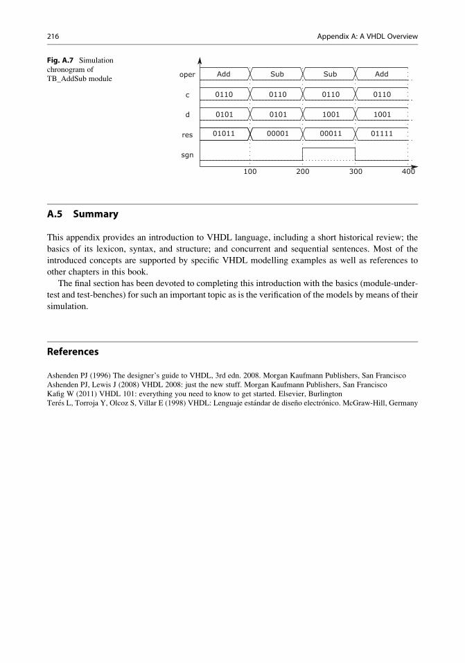
Figure A.7 shows the results of simulation once the events scheduled by Stimuli process have been

applied to the input ports of the AddSub module every 100 ns until reaching the end of this process.

VHD

L

Test-Bench

ResultsAnalysis

StimuliGeneration

VHD

L

Entity

Architecture

MuT: Module

under Test

Stim

uli

Resu

lts

Complete Test-Bench System

VHD

L

Test-Bench

ResultsAnalysis

StimuliGeneration

VHDL

MuT: AddSub

Complete TB_AddSub System

Stim

uli

Resu

lts

a,bopcode

c,doper

sgnres

signzysis

ReAnal

ltsl

Fig. A.6 Schematic generic view of VHDL test-bench for MuT simulation (left hand). Simplified view of complete

VHDL test-bench for AddSub module simulation (right hand)


A.5 Summary

This appendix provides an introduction to VHDL language, including a short historical review; the

basics of its lexicon, syntax, and structure; and concurrent and sequential sentences. Most of the

introduced concepts are supported by specific VHDL modelling examples as well as references to

other chapters in this book.

The final section has been devoted to completing this introduction with the basics (module-under-

test and test-benches) for such an important topic as is the verification of the models by means of their

simulation.

References

Ashenden PJ (1996) The designer’s guide to VHDL, 3rd edn. 2008. Morgan Kaufmann Publishers, San Francisco

Ashenden PJ, Lewis J (2008) VHDL 2008: just the new stuff. Morgan Kaufmann Publishers, San Francisco

Kafig W (2011) VHDL 101: everything you need to know to get started. Elsevier, Burlington

Teres L, Torroja Y, Olcoz S, Villar E (1998) VHDL: Lenguaje estandar de diseno electronico. McGraw-Hill, Germany

0110

0101

Add

0110

0101

Sub Sub

1001

0110

Add

1001

0110

01011res

d

c

oper

sgn

100 200 300 400

00001 00011 01111

Fig. A.7 Simulation

chronogram of

TB_AddSub module


Appendix B: Pseudocode Guidelinesfor the Description of Algorithms

Merce Rullan

The specification of digital systems by means of algorithms is a central aspect of this course and many

times, in order to define algorithms, we use sequences of instructions very similar to programming

language instructions. This appendix addresses those who do not have previous experience in

language programming such as C, Java, Python, or others, or those who, having this experience,

want to brush up their knowledge.

B.1 Algorithms and Pseudocode

An algorithm is a sequence of operations whose objective is the solution of some problem such as a

complex computation or a control process.

Algorithms can be described using various media such as natural languages, flow diagrams, or

perfectly standardized programming languages. The problem with using natural languages is that they

can sometimes be ambiguous, while the problem of using programming languages is that they can be

too restrictive depending on the type of behavior we want to describe.

Pseudocode is a midpoint:

• It is similar to a programming language but more informal.

• It uses a mix of natural language sentences, programming language instructions, and some

keywords that define basic structures.

B.2 Operations and Control Structures

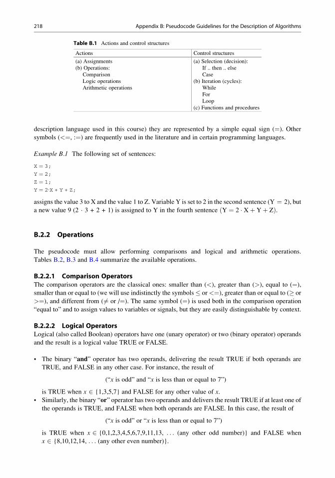
Two important aspects of programming languages and of pseudocode are the actions that can be

performed and the supported control structures. Table B.1 depicts the actions and control structures

of the particular pseudocode used in this book.

B.2.1 Assignments

An assignment is the action of assigning a value to a variable or a signal. In order to avoid confusion

between the symbols that represent the assignment of variables and signals in VHDL (the hardware



description language used in this course) they are represented by a simple equal sign (¼). Other

symbols (<¼, :¼) are frequently used in the literature and in certain programming languages.

Example B.1 The following set of sentences:

X ¼ 3;

Y ¼ 2;

Z ¼ 1;

Y ¼ 2∙X + Y + Z;

assigns the value 3 to X and the value 1 to Z. Variable Y is set to 2 in the second sentence (Y ¼ 2), but

a new value 9 (2 � 3 + 2 + 1) is assigned to Y in the fourth sentence Y ¼ 2 � Xþ Yþ Zð Þ.

B.2.2 Operations

The pseudocode must allow performing comparisons and logical and arithmetic operations.

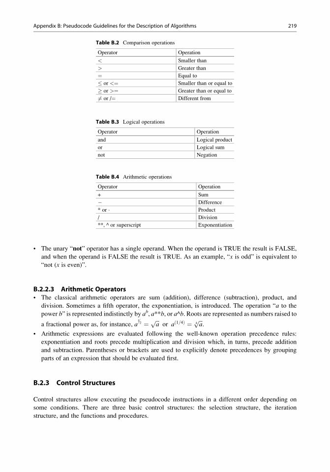
Tables B.2, B.3 and B.4 summarize the available operations.

B.2.2.1 Comparison OperatorsThe comparison operators are the classical ones: smaller than (<), greater than (>), equal to (¼),

smaller than or equal to (we will use indistinctly the symbols� or<¼), greater than or equal to (� or

>¼), and different from ( 6¼ or /¼). The same symbol (¼) is used both in the comparison operation

“equal to” and to assign values to variables or signals, but they are easily distinguishable by context.

B.2.2.2 Logical OperatorsLogical (also called Boolean) operators have one (unary operator) or two (binary operator) operands

and the result is a logical value TRUE or FALSE.

• The binary “and” operator has two operands, delivering the result TRUE if both operands are

TRUE, and FALSE in any other case. For instance, the result of

(“x is odd” and “x is less than or equal to 7”)

is TRUE when x 2 {1,3,5,7} and FALSE for any other value of x.

• Similarly, the binary “or” operator has two operands and delivers the result TRUE if at least one of

the operands is TRUE, and FALSE when both operands are FALSE. In this case, the result of

(“x is odd” or “x is less than or equal to 7”)

is TRUE when x 2 {0,1,2,3,4,5,6,7,9,11,13, . . . (any other odd number)} and FALSE when

x 2 {8,10,12,14, . . . (any other even number)}.

Table B.1 Actions and control structures

Actions Control structures

(a) Assignments

(b) Operations:

Comparison

Logic operations

Arithmetic operations

(a) Selection (decision):

If .. then .. else

Case

(b) Iteration (cycles):

While

For

Loop

(c) Functions and procedures

218 Appendix B: Pseudocode Guidelines for the Description of Algorithms

• The unary “not” operator has a single operand. When the operand is TRUE the result is FALSE,

and when the operand is FALSE the result is TRUE. As an example, “x is odd” is equivalent to

“not (x is even)”.

B.2.2.3 Arithmetic Operators• The classical arithmetic operators are sum (addition), difference (subtraction), product, and

division. Sometimes a fifth operator, the exponentiation, is introduced. The operation “a to the

power b” is represented indistinctly by ab, a**b, or a^b. Roots are represented as numbers raised to

a fractional power as, for instance, a1=2 ¼ ffiffiffi

ap

or a 1=4ð Þ ¼ ffiffiffia4

p.

• Arithmetic expressions are evaluated following the well-known operation precedence rules:

exponentiation and roots precede multiplication and division which, in turns, precede addition

and subtraction. Parentheses or brackets are used to explicitly denote precedences by grouping

parts of an expression that should be evaluated first.

B.2.3 Control Structures

Control structures allow executing the pseudocode instructions in a different order depending on

some conditions. There are three basic control structures: the selection structure, the iteration

structure, and the functions and procedures.

Table B.2 Comparison operations

Operator Operation

< Smaller than

> Greater than

¼ Equal to

� or <¼ Smaller than or equal to

� or >¼ Greater than or equal to

6¼ or /¼ Different from

Table B.3 Logical operations

Operator Operation

and Logical product

or Logical sum

not Negation

Table B.4 Arithmetic operations

Operator Operation

+ Sum

� Difference

* or � Product

/ Division

**, ^ or superscript Exponentiation

Appendix B: Pseudocode Guidelines for the Description of Algorithms 219

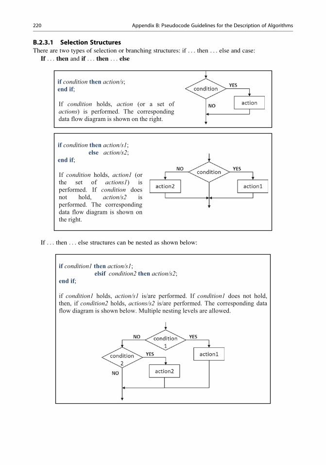
B.2.3.1 Selection StructuresThere are two types of selection or branching structures: if . . . then . . . else and case:

If . . . then and if . . . then . . . else

if condition then action/s;end if;

If condition holds, action (or a set of actions) is performed. The corresponding data flow diagram is shown on the right.

if condition then action/s1;else action/s2;

end if;

If condition holds, action1 (or the set of actions1) is performed. If condition does not hold, action/s2 is performed. The corresponding data flow diagram is shown onthe right.

If . . . then . . . else structures can be nested as shown below:

if condition1 then action/s1;elsif condition2 then action/s2;

end if;

if condition1 holds, action/s1 is/are performed. If condition1 does not hold, then, if condition2 holds, actions/s2 is/are performed. The corresponding data flow diagram is shown below. Multiple nesting levels are allowed.


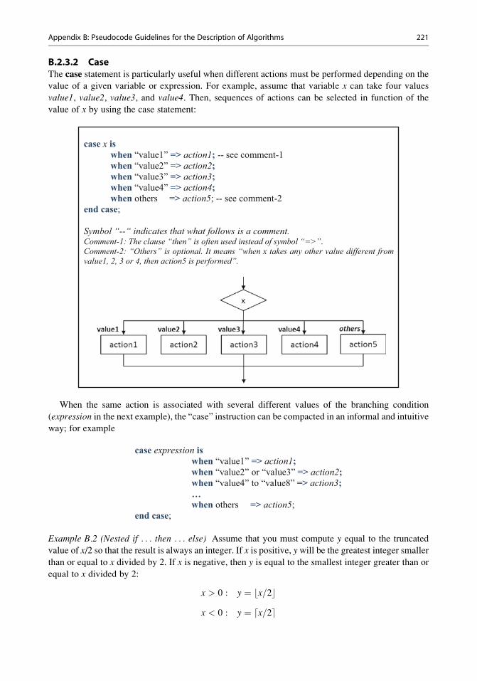
B.2.3.2 CaseThe case statement is particularly useful when different actions must be performed depending on the

value of a given variable or expression. For example, assume that variable x can take four values

value1, value2, value3, and value4. Then, sequences of actions can be selected in function of the

value of x by using the case statement:

case x iswhen “value1” => action1; -- see comment-1when “value2” => action2;when “value3” => action3;when “value4” => action4;when others => action5; -- see comment-2

end case;

Symbol “--“ indicates that what follows is a comment. Comment-1: The clause “then” is often used instead of symbol “=>”.Comment-2: “Others” is optional. It means “when x takes any other value different from value1, 2, 3 or 4, then action5 is performed”.

When the same action is associated with several different values of the branching condition

(expression in the next example), the “case” instruction can be compacted in an informal and intuitive

way; for example

case expression iswhen “value1” => action1;when “value2” or “value3” => action2;when “value4” to “value8” => action3;…when others => action5;

end case;

Example B.2 (Nested if . . . then . . . else) Assume that you must compute y equal to the truncated

value of x/2 so that the result is always an integer. If x is positive, ywill be the greatest integer smaller

than or equal to x divided by 2. If x is negative, then y is equal to the smallest integer greater than or

equal to x divided by 2:

x > 0 : y ¼ x=2b cx < 0 : y ¼ x=2d e


Thus, if

• x is even, then y ¼ x=2;• x is odd and positive, then y ¼ x� 1ð Þ=2 ;

• x is odd and negative, then y ¼ xþ 1ð Þ=2.

For example, if x ¼ 10 then y ¼ 10=2 ¼ 5 and if x ¼ �10 then y ¼ �10=2 ¼ �5; if x ¼ 7 then

y ¼ 7� 1ð Þ=2 ¼ 3; if x ¼ �7 then y ¼ �7þ 1ð Þ=2 ¼ �3.

Thus, the following algorithm computes the integer value of x/2:

if (x is even) then y = x/2;elsif (x is negative) then y = (x+1)/2;else y = (x -1)/2;

end if;Example B.3 (Case) Let us see a second example. Assume x 2 {0,1,2,3,4,5,6,7,8,9} and you want to

generate the binary representation of x : y ¼ x2. The binary numbering system is explained in

Appendix C. A straightforward solution is to consult Table C.1: it gives the equivalence between

the representation of naturals 0–15 in base 10 and in base 2. The entries of Table C.1 that correspond

to numbers 0–9 can be easily described by the following case statement:

case x iswhen 0 => y=0000;when 1 => y=0001;when 2 => y=0010;when 3 => y=0011;when 4 => y=0100;when 5 => y=0101;when 6 => y=0110;when 7 => y=0111;when 8 => y=1000;when 9 => y=1001;

end case;

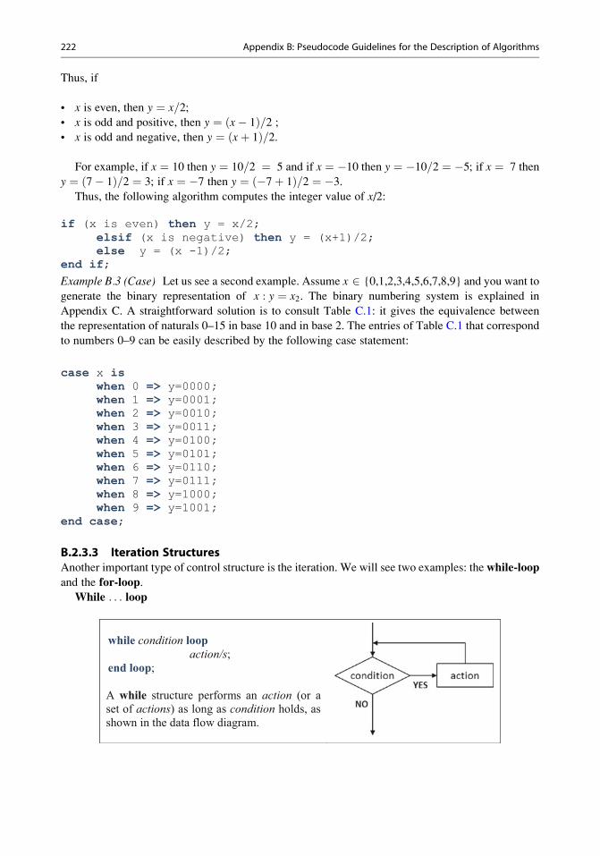
B.2.3.3 Iteration StructuresAnother important type of control structure is the iteration. We will see two examples: the while-loop

and the for-loop.

While . . . loop

while condition loopaction/s;

end loop;

A while structure performs an action (or a set of actions) as long as condition holds, as shown in the data flow diagram.


For . . . loop

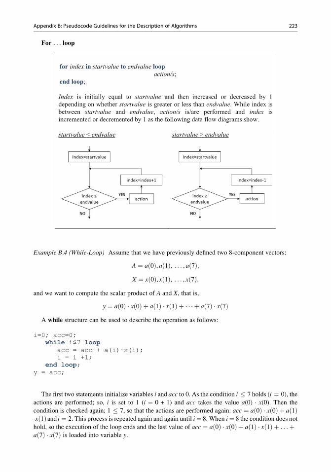
for index in startvalue to endvalue loopaction/s;

end loop;

Index is initially equal to startvalue and then increased or decreased by 1 depending on whether startvalue is greater or less than endvalue. While index is between startvalue and endvalue, action/s is/are performed and index is incremented or decremented by 1 as the following data flow diagrams show.

startvalue < endvalue startvalue > endvalue

Example B.4 (While-Loop) Assume that we have previously defined two 8-component vectors:

A ¼ a 0ð Þ, a 1ð Þ, . . . , a 7ð Þ;X ¼ x 0ð Þ, x 1ð Þ, . . . , x 7ð Þ;

and we want to compute the scalar product of A and X, that is,

y ¼ a 0ð Þ � x 0ð Þ þ a 1ð Þ � x 1ð Þ þ � � � þ a 7ð Þ � x 7ð ÞA while structure can be used to describe the operation as follows:

i=0; acc=0;while i≤7 loop

acc = acc + a(i)∙x(i);i = i +1;

end loop;y = acc;

The first two statements initialize variables i and acc to 0. As the condition i � 7 holds (i ¼ 0), the

actions are performed; so, i is set to 1 (i ¼ 0 + 1) and acc takes the value a(0) � x(0). Then the

condition is checked again; 1 � 7, so that the actions are performed again: acc ¼ a 0ð Þ � x 0ð Þ þ a 1ð Þ�x 1ð Þand i ¼ 2. This process is repeated again and again until i¼ 8. When i¼ 8 the condition does not

hold, so the execution of the loop ends and the last value of acc ¼ a 0ð Þ � x 0ð Þ þ a 1ð Þ � x 1ð Þ þ . . .þa 7ð Þ � x 7ð Þ is loaded into variable y.


Example B.5 (For-Loop) The same computation y ¼ a 0ð Þ � x 0ð Þ þ a 1ð Þ � x 1ð Þ þ � � � þ a 7ð Þ � x 7ð Þcanbe performed using a for . . . loop structure:

acc=0;for i in 0 to 7 loop

acc = acc + a(i)∙x(i);end loop;y = acc;

Index i is initially set to 0 and automatically incremented by 1 each time the loop is executed. As

acc has been initialized to 0, the first time the loop is executed i ¼ 0 and acc ¼ a 0ð Þ � x 0ð Þ. The lasttime the loop is executed is when i ¼ 7 and thus acc ¼ a 0ð Þ � x 0ð Þ þ a 1ð Þ � x 1ð Þ þ . . .þ a 7ð Þ � x 7ð Þ.At this point the loop ends and the last value of acc is loaded into y.

B.2.3.4 Functions and ProceduresFunctions and procedures, also called subroutines, are blocks of pseudocode performing a specific

computation that can be used more than once in other parts of the pseudocode.

The difference between functions and procedures can be sometimes confusing. For example, in

Pascal, a procedure is a function that does not return a value. In C, everything is a function, but if it

does not return a value, it is a “void” function. We will use the most commonly accepted meaning for

those terms. A function is a block of pseudocode that computes a mathematical function and returns a

result. A procedure is a block of pseudocode that performs some task and returns the control to the

main algorithm when finished. Let us see both more deeply.

B.2.3.5 FunctionA function is formally defined as follows:

function name (formal input parameters)……return (expression or value);…

end function;

Within the main algorithm a function is called by writing its name and by giving actual values to

the formal parameters:

. . .x ¼ name (actual input parameters);

. . .

The value computed within the function is assigned to variable x. The call can also be a part of an

expression:

. . .

x ¼ 2 � (name (actual input parameters))2;. . .


In this case the value computed within the function is squared and multiplied by 2 before being

assigned to variable x.

Example B.6 (Function) Assume that we have defined the following function:

function test (x, y, data1, data2)if (x2 - 2∙y) < 0 then return (data1 - data2);else return (data1 + data2);end if;

end function;

and we use the function in the following main pseudocode program:

. . .

a ¼ test (in1, in2, 5, 4);

b ¼ a � test (in3, in4, 0, 8);

c ¼ a + b;

. . .

The result of these sentences when in1 ¼ 8, in2 ¼ 4, in3 ¼ 2, and in4 ¼ 15 will be a ¼ 9

because (in12 � 2 � in2) is a positive number and 5+4 ¼ 9, and b ¼ �72 so that (in32 � 2 � in4)is less than 0 and 9.(0 � 8) ¼ �72.

B.2.3.6 ProcedureA procedure is defined by a name and by an optional set of formal parameters:

procedure name (formal parameters)…(return)…

end procedure;

When a procedure is called, the list of formal parameters is substituted by the actual parameters:

variables used as operands within the procedure computations (input parameters) and variables whose

values are updated with procedure computation results (output parameters). Every time the procedure

finds a “return” or an “end procedure” sentence, the flow control goes back to the piece of pseudocode

from which it was called, more precisely to the sentence below the call.

The procedure can be called from any piece of pseudocode simply by writing its name and the list

of values with which computations will be done (actual parameters):

name (actual parameters)

Example B.7 (Procedure) Let us see an example: we want to compute the value of

z ¼ a:ffiffiffix

p þ b:ffiffiffiy

p

with an accuracy of 16 fractional digits. An algorithm computing the square root of a number can be

developed and encapsulated within a procedure “square_root” with parameters x, y, and n. Procedure

square_root will compute the square root of x with n fractional digits and will return the result into y.


procedure square_root (x, y, n)……

end procedure;

Now, this procedure can be used in the main algorithm to compute the square root of x and the

square root of y without writing twice the sentences necessary to calculate the square root:

square_root (x,u,16);-- computes u ←ffiffiffix

pwith accuracy¼16

u ¼ u � a; -- u ← a:ffiffiffix

psquare_root (y,v,16); -- computes v ←

ffiffiffiy

pwith accuracy¼16

v ¼ b : v; -- v ← b:ffiffiffiy

pz ¼ u þ v; -- z ¼ a:

ffiffiffix

p þ b:ffiffiffiy

p. . .

The use of procedures not only facilitates the design of pseudocode but also improves the

understanding avoiding the unnecessary repetition of sentences.


Appendix C: Binary Numeration System

Merce Rullan

Computers and other electronic systems receive, store, process, and transmit data of different types:

numbers, characters, sounds, pictures, etc. The common point is that all those data are encoded using

0s and 1s because computer technology relies on devices having two stable states which are

associated with bits (binary digits) 0 and 1, respectively. In particular, numbers must also be

represented by 0s and 1s, and the binary numeration system (base 2) offers the possibility not only

to represent numbers but also to perform arithmetic operations using well-known and reliable

algorithms.

This appendix is a short review of those fundamental concepts of the binary numeration system

that all digital systems designer should know. Due to the convenience, sometimes, of expressing the

numbers in a more compact form, a brief explanation of the hexadecimal system has been included.

C.1 Numeration Systems

Most commonly used numeration systems are positional: numbers are represented by strings

(sequences) of digits and a weight is associated with every digit position. For example, in decimal

(base 10 numeration system), 663 represents the following number:

663 ¼ 6 � 102 þ 6 � 101 þ 3 � 100

Thus, in the preceding expression, digit 6 has two different weights depending on its position: the

leftmost 6, located in the position of the hundreds, has a weight equal to 102, while the 6 in the middle,

located in the position of the tens, has a weight equal to 101.

The decimal system uses 10 digits 0, 1, 2, 3, 4, 5, 6, 7, 8, and 9, and the n-digit sequence xn�1 xn�2

. . . x1 x0 represents the number

X ¼Xn�1

i¼0

xi � 10i

More generally, the base b numeration system, being b � 2 a natural (non-negative integer), uses

b digits 0, 1, 2, . . ., b � 1. The weights associated with each digit position, starting with the rightmost

digit, are b0, b1, b2, b3, . . . and so on. Thus, the base-b n-digit sequence xn�1 xn�2 . . . x1 x0 represents

the number



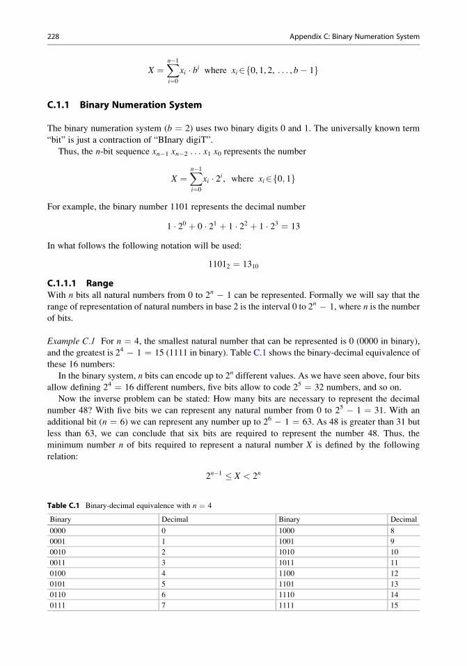
X ¼Xn�1

i¼0

xi � bi where xi2 0, 1, 2, . . . , b� 1f g

C.1.1 Binary Numeration System

The binary numeration system (b ¼ 2) uses two binary digits 0 and 1. The universally known term

“bit” is just a contraction of “BInary digiT”.

Thus, the n-bit sequence xn�1 xn�2 . . . x1 x0 represents the number

X ¼Xn�1

i¼0

xi � 2i, where xi2 0; 1f g

For example, the binary number 1101 represents the decimal number

1 � 20 þ 0 � 21 þ 1 � 22 þ 1 � 23 ¼ 13

In what follows the following notation will be used:

11012 ¼ 1310

C.1.1.1 RangeWith n bits all natural numbers from 0 to 2n � 1 can be represented. Formally we will say that the

range of representation of natural numbers in base 2 is the interval 0 to 2n � 1, where n is the number

of bits.

Example C.1 For n ¼ 4, the smallest natural number that can be represented is 0 (0000 in binary),

and the greatest is 24 � 1 ¼ 15 (1111 in binary). Table C.1 shows the binary-decimal equivalence of

these 16 numbers:

In the binary system, n bits can encode up to 2n different values. As we have seen above, four bits

allow defining 24 ¼ 16 different numbers, five bits allow to code 25 ¼ 32 numbers, and so on.

Now the inverse problem can be stated: How many bits are necessary to represent the decimal

number 48? With five bits we can represent any natural number from 0 to 25 � 1 ¼ 31. With an

additional bit (n ¼ 6) we can represent any number up to 26 � 1 ¼ 63. As 48 is greater than 31 but

less than 63, we can conclude that six bits are required to represent the number 48. Thus, the

minimum number n of bits required to represent a natural number X is defined by the following

relation:

2n�1 � X < 2n

Table C.1 Binary-decimal equivalence with n ¼ 4

Binary Decimal Binary Decimal

0000 0 1000 8

0001 1 1001 9

0010 2 1010 10

0011 3 1011 11

0100 4 1100 12

0101 5 1101 13

0110 6 1110 14

0111 7 1111 15

228 Appendix C: Binary Numeration System

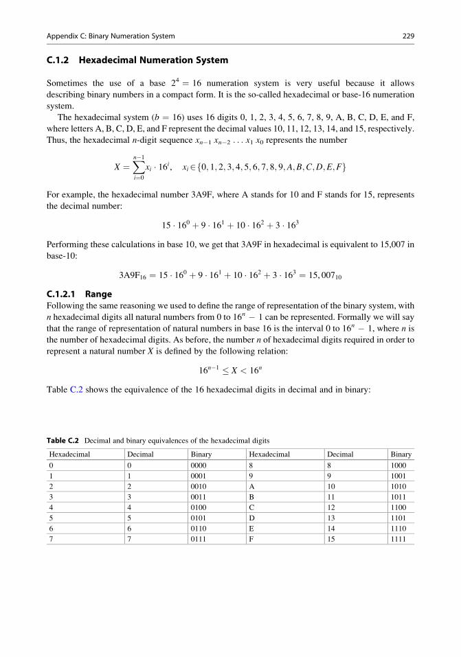
C.1.2 Hexadecimal Numeration System

Sometimes the use of a base 24 ¼ 16 numeration system is very useful because it allows

describing binary numbers in a compact form. It is the so-called hexadecimal or base-16 numeration

system.

The hexadecimal system (b ¼ 16) uses 16 digits 0, 1, 2, 3, 4, 5, 6, 7, 8, 9, A, B, C, D, E, and F,

where letters A, B, C, D, E, and F represent the decimal values 10, 11, 12, 13, 14, and 15, respectively.

Thus, the hexadecimal n-digit sequence xn�1 xn�2 . . . x1 x0 represents the number

X ¼Xn�1

i¼0

xi � 16i, xi2 0; 1; 2; 3; 4; 5; 6; 7; 8; 9;A;B;C;D;E;Ff g

For example, the hexadecimal number 3A9F, where A stands for 10 and F stands for 15, represents

the decimal number:

15 � 160 þ 9 � 161 þ 10 � 162 þ 3 � 163

Performing these calculations in base 10, we get that 3A9F in hexadecimal is equivalent to 15,007 in

base-10:

3A9F16 ¼ 15 � 160 þ 9 � 161 þ 10 � 162 þ 3 � 163 ¼ 15, 00710

C.1.2.1 RangeFollowing the same reasoning we used to define the range of representation of the binary system, with

n hexadecimal digits all natural numbers from 0 to 16n � 1 can be represented. Formally we will say

that the range of representation of natural numbers in base 16 is the interval 0 to 16n � 1, where n is

the number of hexadecimal digits. As before, the number n of hexadecimal digits required in order to

represent a natural number X is defined by the following relation:

16n�1 � X < 16n

Table C.2 shows the equivalence of the 16 hexadecimal digits in decimal and in binary:

Table C.2 Decimal and binary equivalences of the hexadecimal digits

Hexadecimal Decimal Binary Hexadecimal Decimal Binary

0 0 0000 8 8 1000

1 1 0001 9 9 1001

2 2 0010 A 10 1010

3 3 0011 B 11 1011

4 4 0100 C 12 1100

5 5 0101 D 13 1101

6 6 0110 E 14 1110

7 7 0111 F 15 1111

Appendix C: Binary Numeration System 229

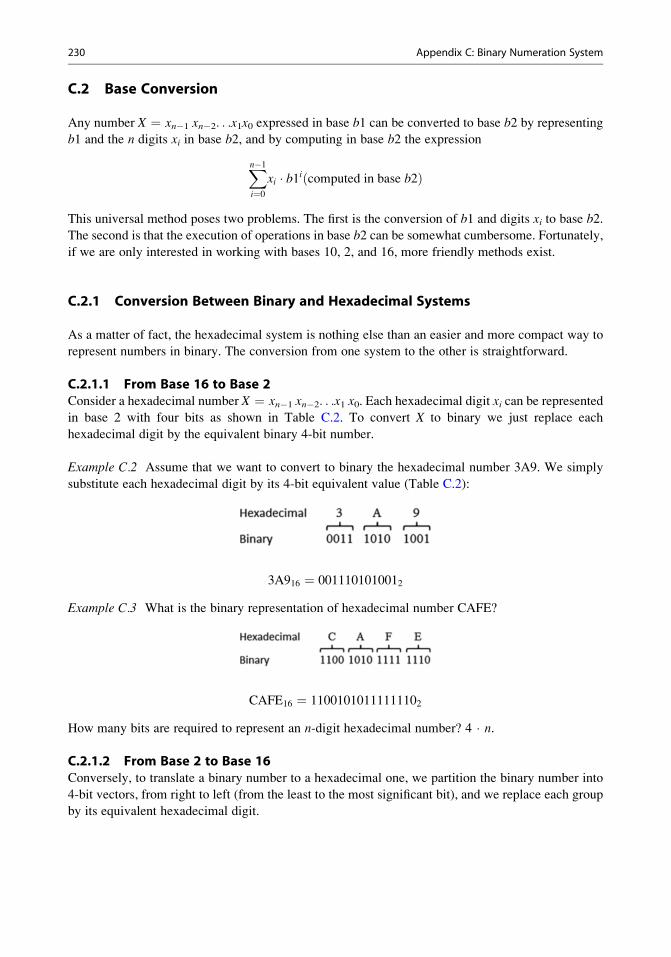
C.2 Base Conversion

Any number X ¼ xn�1 xn�2. . .x1x0 expressed in base b1 can be converted to base b2 by representing

b1 and the n digits xi in base b2, and by computing in base b2 the expression

Xn�1

i¼0

xi � b1i computed in base b2ð Þ

This universal method poses two problems. The first is the conversion of b1 and digits xi to base b2.

The second is that the execution of operations in base b2 can be somewhat cumbersome. Fortunately,

if we are only interested in working with bases 10, 2, and 16, more friendly methods exist.

C.2.1 Conversion Between Binary and Hexadecimal Systems

As a matter of fact, the hexadecimal system is nothing else than an easier and more compact way to

represent numbers in binary. The conversion from one system to the other is straightforward.

C.2.1.1 From Base 16 to Base 2Consider a hexadecimal number X ¼ xn�1 xn�2. . .x1 x0. Each hexadecimal digit xi can be represented

in base 2 with four bits as shown in Table C.2. To convert X to binary we just replace each

hexadecimal digit by the equivalent binary 4-bit number.

Example C.2 Assume that we want to convert to binary the hexadecimal number 3A9. We simply

substitute each hexadecimal digit by its 4-bit equivalent value (Table C.2):

3A916 ¼ 0011101010012

Example C.3 What is the binary representation of hexadecimal number CAFE?

CAFE16 ¼ 11001010111111102

How many bits are required to represent an n-digit hexadecimal number? 4 � n.

C.2.1.2 From Base 2 to Base 16Conversely, to translate a binary number to a hexadecimal one, we partition the binary number into

4-bit vectors, from right to left (from the least to the most significant bit), and we replace each group

by its equivalent hexadecimal digit.


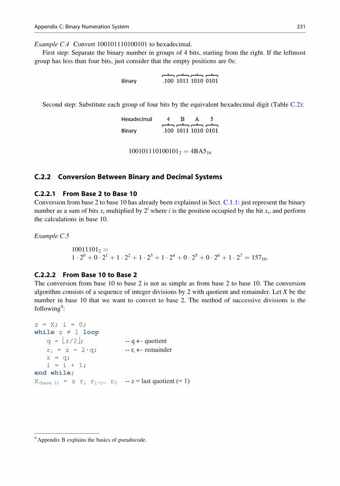
Example C.4 Convert 100101110100101 to hexadecimal.

First step: Separate the binary number in groups of 4 bits, starting from the right. If the leftmost

group has less than four bits, just consider that the empty positions are 0s:

Second step: Substitute each group of four bits by the equivalent hexadecimal digit (Table C.2):

1001011101001012 ¼ 4BA516

C.2.2 Conversion Between Binary and Decimal Systems

C.2.2.1 From Base 2 to Base 10Conversion from base 2 to base 10 has already been explained in Sect. C.1.1: just represent the binary

number as a sum of bits xi multiplied by 2i where i is the position occupied by the bit xi, and perform

the calculations in base 10.

Example C.5

100111012 ¼1 � 20 þ 0 � 21 þ 1 � 22 þ 1 � 23 þ 1 � 24 þ 0 � 25 þ 0 � 26 þ 1 � 27 ¼ 15710:

C.2.2.2 From Base 10 to Base 2The conversion from base 10 to base 2 is not as simple as from base 2 to base 10. The conversion

algorithm consists of a sequence of integer divisions by 2 with quotient and remainder. Let X be the

number in base 10 that we want to convert to base 2. The method of successive divisions is the

following4:

z = X; i = 0; while z ≠ 1 loop

q = ⎣z/2⎦; -- q ← quotientri = z - 2∙q; -- ri ← remainderz = q;i = i + 1;

end while;X(base 2) = z ri ri-1… r0 -- z = last quotient (= 1)

4 Appendix B explains the basics of pseudocode.


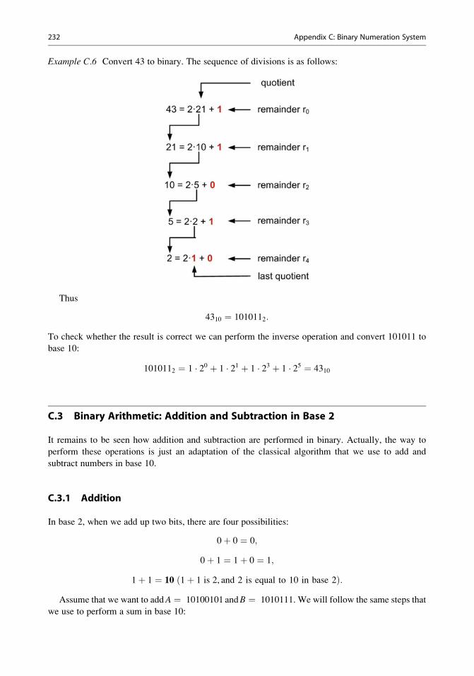
Example C.6 Convert 43 to binary. The sequence of divisions is as follows:

Thus

4310 ¼ 1010112:

To check whether the result is correct we can perform the inverse operation and convert 101011 to

base 10:

1010112 ¼ 1 � 20 þ 1 � 21 þ 1 � 23 þ 1 � 25 ¼ 4310

C.3 Binary Arithmetic: Addition and Subtraction in Base 2

It remains to be seen how addition and subtraction are performed in binary. Actually, the way to

perform these operations is just an adaptation of the classical algorithm that we use to add and

subtract numbers in base 10.

C.3.1 Addition

In base 2, when we add up two bits, there are four possibilities:

0þ 0 ¼ 0;

0þ 1 ¼ 1þ 0 ¼ 1;

1þ 1 ¼ 10 ð1þ 1 is 2, and 2 is equal to 10 in base 2Þ:Assume that we want to addA ¼ 10100101 andB ¼ 1010111. We will follow the same steps that

we use to perform a sum in base 10:


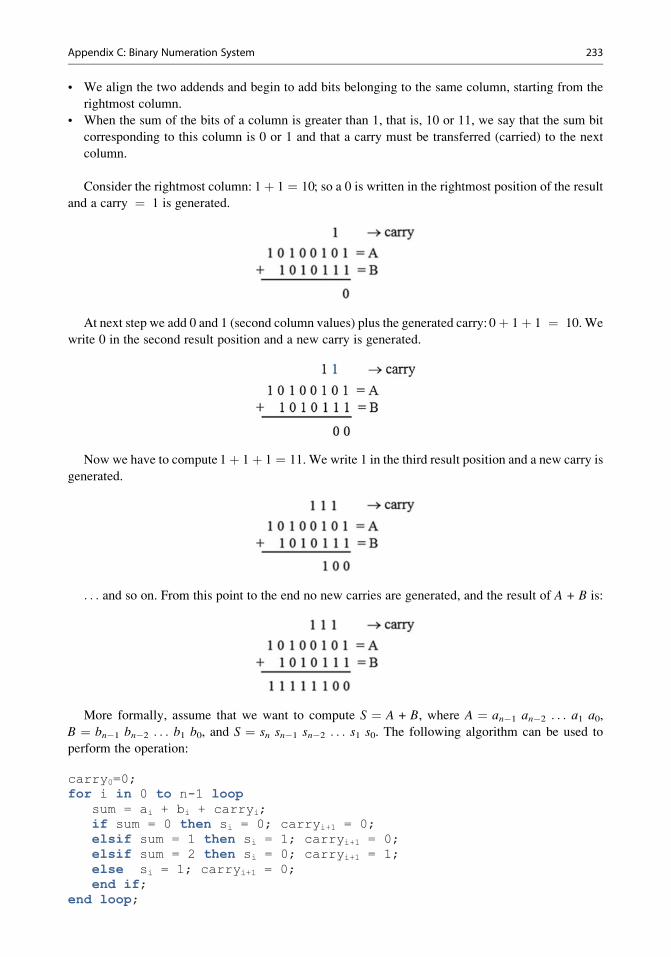
• We align the two addends and begin to add bits belonging to the same column, starting from the

rightmost column.

• When the sum of the bits of a column is greater than 1, that is, 10 or 11, we say that the sum bit

corresponding to this column is 0 or 1 and that a carry must be transferred (carried) to the next

column.

Consider the rightmost column: 1þ 1 ¼ 10; so a 0 is written in the rightmost position of the result

and a carry ¼ 1 is generated.

At next step we add 0 and 1 (second column values) plus the generated carry: 0þ 1þ 1 ¼ 10. We

write 0 in the second result position and a new carry is generated.

Now we have to compute 1þ 1þ 1 ¼ 11. We write 1 in the third result position and a new carry is

generated.

. . . and so on. From this point to the end no new carries are generated, and the result of A + B is:

More formally, assume that we want to compute S ¼ A + B, where A ¼ an�1 an�2 . . . a1 a0,

B ¼ bn�1 bn�2 . . . b1 b0, and S ¼ sn sn�1 sn�2 . . . s1 s0. The following algorithm can be used to

perform the operation:

carry0=0;for i in 0 to n-1 loop

sum = ai + bi + carryi;if sum = 0 then si = 0; carryi+1 = 0;elsif sum = 1 then si = 1; carryi+1 = 0;elsif sum = 2 then si = 0; carryi+1 = 1;else si = 1; carryi+1 = 0;end if;

end loop;


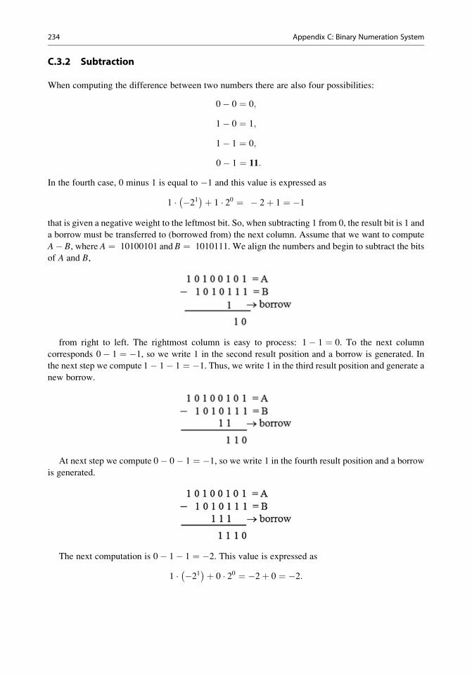
C.3.2 Subtraction

When computing the difference between two numbers there are also four possibilities:

0� 0 ¼ 0;

1� 0 ¼ 1;

1� 1 ¼ 0;

0� 1 ¼ 11:

In the fourth case, 0 minus 1 is equal to �1 and this value is expressed as

1 � �21� �þ 1 � 20 ¼ � 2þ 1 ¼ �1

that is given a negative weight to the leftmost bit. So, when subtracting 1 from 0, the result bit is 1 and

a borrow must be transferred to (borrowed from) the next column. Assume that we want to compute

A� B, where A ¼ 10100101 and B ¼ 1010111. We align the numbers and begin to subtract the bits

of A and B,

from right to left. The rightmost column is easy to process: 1� 1 ¼ 0. To the next column

corresponds 0� 1 ¼ �1, so we write 1 in the second result position and a borrow is generated. In

the next step we compute 1� 1� 1 ¼ �1. Thus, we write 1 in the third result position and generate a

new borrow.

At next step we compute 0� 0� 1 ¼ �1, so we write 1 in the fourth result position and a borrow

is generated.

The next computation is 0� 1� 1 ¼ �2. This value is expressed as

1 � �21� �þ 0 � 20 ¼ �2þ 0 ¼ �2:


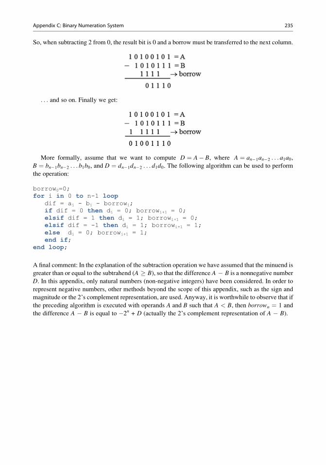
So, when subtracting 2 from 0, the result bit is 0 and a borrow must be transferred to the next column.

. . . and so on. Finally we get:

More formally, assume that we want to compute D ¼ A� B, where A ¼ an�1an�2 . . . a1a0,B ¼ bn�1bn�2 . . . b1b0, and D ¼ dn�1dn�2 . . . d1d0. The following algorithm can be used to perform

the operation:

borrow0=0;for i in 0 to n-1 loop

dif = ai - bi - borrowi;if dif = 0 then di = 0; borrowi+1 = 0;elsif dif = 1 then di = 1; borrowi+1 = 0;elsif dif = -1 then di = 1; borrowi+1 = 1;else di = 0; borrowi+1 = 1;end if;

end loop;

A final comment: In the explanation of the subtraction operation we have assumed that the minuend is

greater than or equal to the subtrahend (A � B), so that the difference A � B is a nonnegative number

D. In this appendix, only natural numbers (non-negative integers) have been considered. In order to

represent negative numbers, other methods beyond the scope of this appendix, such as the sign and

magnitude or the 2’s complement representation, are used. Anyway, it is worthwhile to observe that if

the preceding algorithm is executed with operands A and B such that A < B, then borrown ¼ 1 and

the difference A � B is equal to �2n + D (actually the 2’s complement representation of A � B).


Index

AAccess control system, 79

Adder

binary, 69

1-bit, 24, 40

4-bit, 21, 24, 34

n-bit, 691-digit, 7

2-digit, 5

half, 102

1-operand, 102

Adder/subtractor

binary, 71

n-bit, 71

sign-magnitude, 76

Addition

binary, 23

pencil and paper algorithm, 69

Address decoder, 61, 107

Addressing space, 111

Adjacency, 47

Algorithm

binary decision, 62

paper and pencil, 6

sequential implementation, 113

Alphabet

input, 119

output, 119

Anti-fuse, 187

Application specific integrated circuit, 180

Architecture

stored program, 144

von Neumann, 144

Assignment

memory, 139

port, 138, 141

Asynchronous input, 93

reset, 93

set, 93

Asynchronous sequential circuit, 90, 91

BBinary coded decimal, 42

Bistable component, 88

Bit line, 107

Boolean algebra

binary, 28

duality principle, 28

neutral elements, 27

postulates, 27

properties, 30

Boolean expression, 31

Borrow

incoming, 70

outgoing, 70

Buffer, 17

3-state, 17

tri-state, 41, 61

Bus, 61

address, 107, 109

4-bit, 41

data, 109

CCanonical representation, 32

Carry

incoming, 21, 69

outgoing, 22, 69

Cell

programmable, 185

uncommitted, 185

Chip, 179

Chronometer, 3, 135, 140

program, 141

simulation, 166

Circuit structure

technology independent, 188

Clock

active-high, 98

active-low, 98

Clock signal, 82

Codification, binary, 11

Combinational circuit, 21

gate implementation, 31

ROM implementation, 23

Comparator, n-bit, 512’s Complement

representation, 70



Component, 7

electronic, 11–17

sequential, 96

Computation resource, 137

Conditional branch, 62

Conditional switch, 63

Configurable logic block, 187

Connection, programmable, 185

Control input, asynchronous, 97

Conversion

parallel-to-serial, 100

serial-to-parallel, 100

Conversion function, 109

conv_integer, 156Counter

BCD, 101

bidirectional, 101, 103

down, 101

Gray, 101

mod m, 101m-state, 101programmable, 104

up, 101

up/down, 103

Cube, 45

adjacent, 47

Cycle, 82

DDecoder

address, 61

BCD to 7-segment, 42

Decrementer, 76

Delay, 50

Description

explicit functional, 33, 83

functional, 4–7

hierarchical, 8

implicit, 5

implicit functional, 33

2-level hierarchical, 8

3-level hierarchical, 8

structural, 7

Design method, 171

Die, silicon, 181

Digit, quaternary, 52

Digital electronic systems, 10–18

Divider

binary, 74, 76

frequency, 106

Division, 74

accuracy, 74

by 2, 98

error, 74

Don’t care, 42

EEdge

negative, 82

positive, 82

Electronic design automation tool, 172, 175

FFeedthrough cell, 185

Field programmable device, 60

Field programmable gate array, 24, 59, 185

configuration data, 187

Finite state machine, 119

Mealy, 120

Moore, 120

VHDL model, 121

Flip-flop, 88, 91

with asynchronous inputs, 93

D-type, 91

JK, 93

SR, 93

T, 93

Floating gate transistor, 187

Floor plan, 185

FPGA, 185

Flow diagram, 139

Frequency, 82

Frequency divider, 106

Full adder, 69

Full subtractor (FS), 71

Function

next-state, 119

output, 119

switching, 21

GGate

AND3, 16

2-input AND, 16

2-input NAND, 14

2-input NOR, 15

2-input OR, 16

k-input NAND, 35k-input NOR, 35NAND2, 35

NAND3, 16

NOR2, 35

NOR3, 16

OR3, 16

XNOR, 37

XOR, 37

Gate array, 185

channel less, 185

HHalf adder, 102

High level synthesis tool, 175

IIC production line, 182

Implementation

combinational vs. sequential, 116physical, 179

top-down, 150

Implementation strategy, standard cell, 184

Incrementer, 76

Input, asynchronous, 93

Input port, 137

238 Index

Input/output, programmable, 185

Instruction

case, 63

decoder, 161

function call, 65

if then else, 62

for loop, 64

procedure call, 65

while loop, 64

Instruction type, 139

code, 143

encoding, 160

parameters, 143

Integrated circuit

application specific, 180

large scale, 179, 180

medium scale, 179

package, 181

small scale, 179

Integration density, 182

Inverter

CMOS, 13

tri-state, 41

KKarnaugh map, 48

LLatch, 88

D-type, 89

enable input, 89

load input, 89

SR, 90

Latch vs. flip-flop, 92Layout, 182

CMOS inverter, 182

NAND3, 184

NAND4, 185

Literal, 32

Logic synthesis, 188

Look up table, 24, 59, 187

MMacrocell

memory, 157, 184

mutltiplier, 184

processor, 184

Magnitude comparator, 52

2-bit, 54

4-bit, 39

Manufacturing

dicing, 182

etching, 181

ion implementation, 181

oxidation, 181

Mealy model, 84, 85, 95

Memory, 107

anti-fuse technology, 110

bank, 111

1-bit, 89, 90

bit line, 109

DRAM, 108, 109

EEPROM, 110

EPROM, 110

flash, 110

fuse technology, 110

mask programmable, 110

non-volatile, 108

NVRAM, 108

OTP, 110

PROM, 110

RAM, 108, 109

read/write, 108

refresh, 109

reprogrammable, 110

ROM, 108, 110

SRAM, 108, 109

storage permanence, 108

structure, 107

types, 108

user programmable, 110

word line, 109

Microelectronics, 181

Minterm, 32

Moore model, 84, 85, 87

Multiplexer

2-to-1, 55

k-to-1, 55

Multiplication, by 2, 98

Multiplier

binary, 72

1-bit, 76

n-bit by m-bit, 77

NNegative edge triggered, 83

Next state table, 88

OOperation scheduling, 171

Output enable, 97

active-high, 98

active-low, 98

Output port, 137

Output table, 88

PPackage, 181

window, 110

Parallel output, 98

Parity bit, 39

Physical implementation, 179, 188

Physical system, 1

Placement, 188

Plane

AND, 60

OR, 60

Positive edge triggered, 83

Index 239

Pragma, 176

Printed circuit board, 179

surface-mount device, 179

surface mount technology, 179

through-hole technology, 179

Procedure call, 65

Processor, 135, 160

behavior, 144

block diagram, 145

complete circuit, 161

computation resource, 146, 149, 152

functional specification, 143, 144

go to, 146, 149, 158

high level functional specification, 175

input selection, 146, 147, 150

logic synthesis, 171

output selection, 146, 147, 153

register bank, 146, 148, 155

RTL behavioral description, 172

RTL description, 171

scheduling, 173

simulation, 166

structural description, 171

structural specification, 145

synthesis, 172, 175

test, 164

timing specification, 173

top-down implementation, 145

VHDL model, 161

Program counter, 104

Programmable array of logic, 61

Programmable counter, 146

Programmable logic array, 61

Programmable logic device, 61

Programmable resource, 118

Programmable timer, 126

Programming language, 62

Propagation time, 50

Prototyping board, 179

Pseudo-code, 2

Pulse

negative, 82

positive, 82

RRead only memory (ROM), 17, 22, 61, 108

EEPROM, 108

EPROM, 108

flash, 108

mask programmable, 108

one time programmable, 108

OTP, 108

Reducer, mod m, 77Redundant term, 42

Register

n-bit, 97parallel, 97

shift, 98

Register transfer level description, 188

Register transfer level model, 171

Representation, cube, 45

Reset

asynchronous, 105

synchronous, 105

Resource

computation, 128

programmable, 118

Robot control circuit, 93

next state table, 88

output table, 88

Robot vacuum cleaner, 86

ROM. See Read only memory (ROM)

Routing, 188

Routing channel, 185

SSea of gates, 185

Sequence detection, 100

Sequence detector, 80

implementation, 82

Sequence generator, 81, 106

Sequence recognition, 129

Sequential circuit, 79, 80

external input, 81

external output, 81

general structure, 81

internal state, 81

next state, 81

synchronization, 82

Sequential component, 96

Serial input, 98

Set up time, 120

Shift register, 98

bidirectional, 98

clock enable signal, 99

cyclic, 98

left, 98

output enable signal, 99

parallel input, 98, 99

parallel load signal, 99

parallel output, 98, 99

right, 98

serial input, 98, 99

serial output, 98

Signal

analog, 3

digital, 3

discrete, 3

Silicon die, 181, 182

Silicon foundry, 182

Silicon slice, 182

Silicon wafer, 182

Specification

explicit, 5, 6, 22

functional, 2

implicit, 6

Square root, 113

iterative circuit, 114

sequential implementation, 115

State transition graph, 83, 86

Subcube, 45

Substrate, silicon, 181

240 Index

Subtraction, pencil and paper algorithm, 70

Subtractor

binary, 70

n-bit, 70, 71Switch

nMOS, 12

pMOS, 12

Switching function, n-variable, 29Switching function synthesis

with AND and OR planes, 60

with LUT, 59

with LUT and multiplexers, 59

with multiplexers, 57

with ROM, 59

Synchronization, 82

Synchronous input, 93

Synthesis, 42

digital electronic system, 18

method, 22, 93

Synthesis tool, combinational circuit, 45

SystemC, 171

TTable

next state, 88

output, 88

Technology mapping, 188

Temperature control, 2, 21

Temperature controller, 135, 138

program, 139, 143

simulation, 166

Timer, programmable, 104

Tool

electronic design automation (EDA), 175, 179

high level synthesis, 175

implementation, 188

logic synthesis, 188

physical implementation, 188

place and route, 184

synthesis, 188

Transistor

MOS, 11

nMOS, 11

pMOS, 11

Truth table, 31

UUniversal module, 35, 56

VVariable extraction, 58

Verilog, 66, 171

VHDL model, 66

complete processor, 161

computation resource, 152

go to, 158

IEEE arithmetic package, 152, 156

input selection, 151

output selection, 154

package main_parameter, 151, 159package program, 164register bank, 156, 157

simulation, 166

test bench, 164

WWell, n-type, 181Word line, 107

Index 241

Documents

Appendix A: A VHDL Overview - Springer978-3-319-41198-9/1.pdf · Appendix A: A VHDL Overview ... variable Increment : integer; signal Clk : bit :¼ ‘1’; Constants and variables