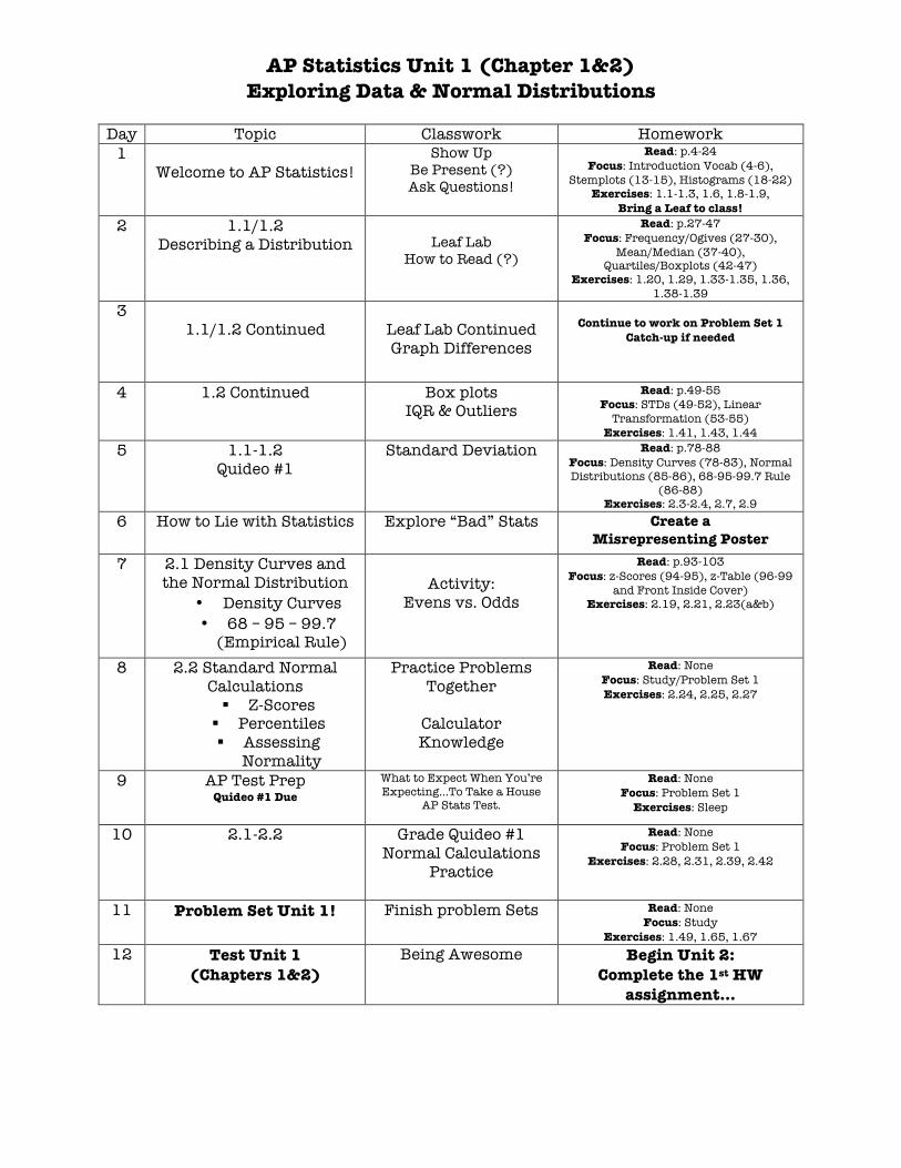
AP Statistics Unit 1 (Chapter 1&2) Exploring Data & Normal Distributions

Day Topic Classwork Homework

1 Welcome to AP Statistics!

Show Up Be Present (?) Ask Questions!

Read: p.4-24 Focus: Introduction Vocab (4-6),

Stemplots (13-15), Histograms (18-22) Exercises: 1.1-1.3, 1.6, 1.8-1.9,

Bring a Leaf to class! 2 1.1/1.2

Describing a Distribution

Leaf Lab

How to Read (?)

Read: p.27-47 Focus: Frequency/Ogives (27-30),

Mean/Median (37-40), Quartiles/Boxplots (42-47)

Exercises: 1.20, 1.29, 1.33-1.35, 1.36, 1.38-1.39

3 1.1/1.2 Continued

Leaf Lab Continued Graph Differences

Continue to work on Problem Set 1

Catch-up if needed

4 1.2 Continued Box plots IQR & Outliers

Read: p.49-55 Focus: STDs (49-52), Linear

Transformation (53-55) Exercises: 1.41, 1.43, 1.44

5 1.1-1.2 Quideo #1

Standard Deviation Read: p.78-88 Focus: Density Curves (78-83), Normal Distributions (85-86), 68-95-99.7 Rule

(86-88) Exercises: 2.3-2.4, 2.7, 2.9

6 How to Lie with Statistics Explore “Bad” Stats Create a Misrepresenting Poster

7 2.1 Density Curves and the Normal Distribution

• Density Curves • 68 – 95 – 99.7

(Empirical Rule)

Activity:

Evens vs. Odds

Read: p.93-103 Focus: z-Scores (94-95), z-Table (96-99

and Front Inside Cover) Exercises: 2.19, 2.21, 2.23(a&b)

8 2.2 Standard Normal Calculations § Z-Scores

§ Percentiles § Assessing

Normality

Practice Problems Together

Calculator Knowledge

Read: None Focus: Study/Problem Set 1 Exercises: 2.24, 2.25, 2.27

9 AP Test Prep Quideo #1 Due

What to Expect When You’re Expecting...To Take a House

AP Stats Test.

Read: None Focus: Problem Set 1

Exercises: Sleep

10 2.1-2.2 Grade Quideo #1 Normal Calculations

Practice

Read: None Focus: Problem Set 1

Exercises: 2.28, 2.31, 2.39, 2.42

11 Problem Set Unit 1!

Finish problem Sets Read: None Focus: Study

Exercises: 1.49, 1.65, 1.67 12 Test Unit 1

(Chapters 1&2)

Being Awesome Begin Unit 2: Complete the 1st HW

assignment…

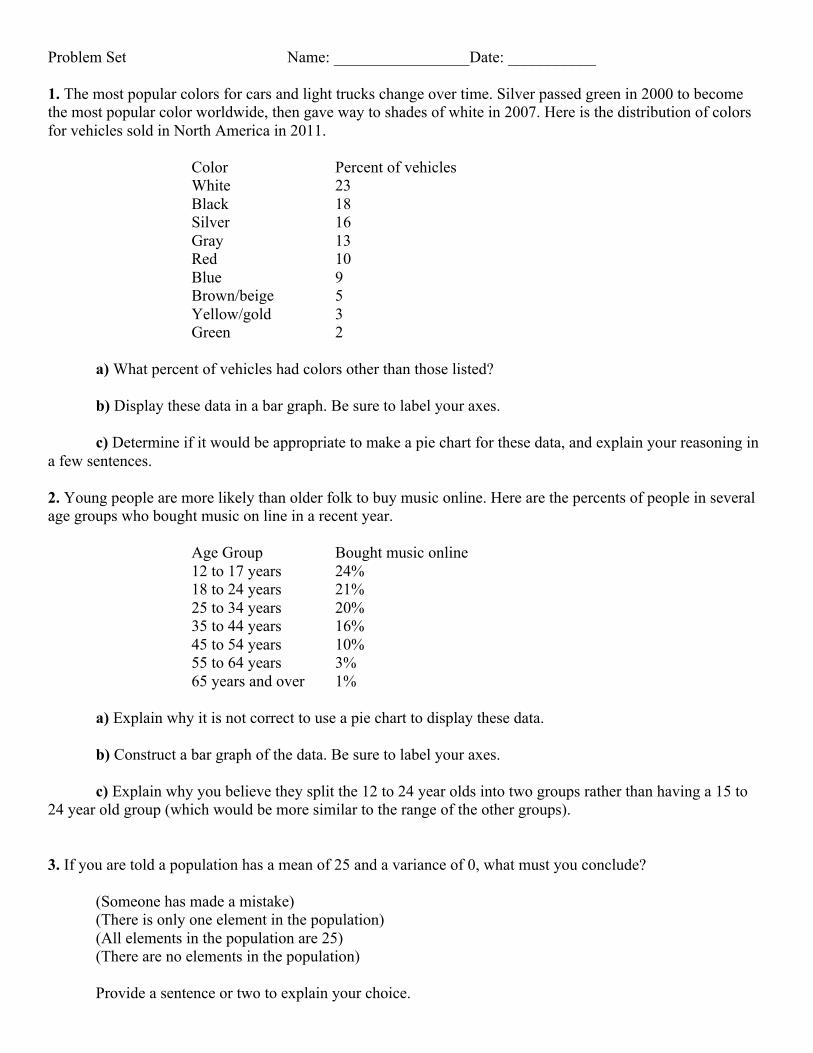
Problem Set Name: _________________Date: ___________ 1. The most popular colors for cars and light trucks change over time. Silver passed green in 2000 to become the most popular color worldwide, then gave way to shades of white in 2007. Here is the distribution of colors for vehicles sold in North America in 2011. Color Percent of vehicles White 23 Black 18 Silver 16 Gray 13 Red 10 Blue 9 Brown/beige 5 Yellow/gold 3 Green 2 a) What percent of vehicles had colors other than those listed? b) Display these data in a bar graph. Be sure to label your axes. c) Determine if it would be appropriate to make a pie chart for these data, and explain your reasoning in a few sentences. 2. Young people are more likely than older folk to buy music online. Here are the percents of people in several age groups who bought music on line in a recent year. Age Group Bought music online 12 to 17 years 24% 18 to 24 years 21% 25 to 34 years 20% 35 to 44 years 16% 45 to 54 years 10% 55 to 64 years 3% 65 years and over 1% a) Explain why it is not correct to use a pie chart to display these data. b) Construct a bar graph of the data. Be sure to label your axes. c) Explain why you believe they split the 12 to 24 year olds into two groups rather than having a 15 to 24 year old group (which would be more similar to the range of the other groups). 3. If you are told a population has a mean of 25 and a variance of 0, what must you conclude? (Someone has made a mistake) (There is only one element in the population) (All elements in the population are 25) (There are no elements in the population) Provide a sentence or two to explain your choice.

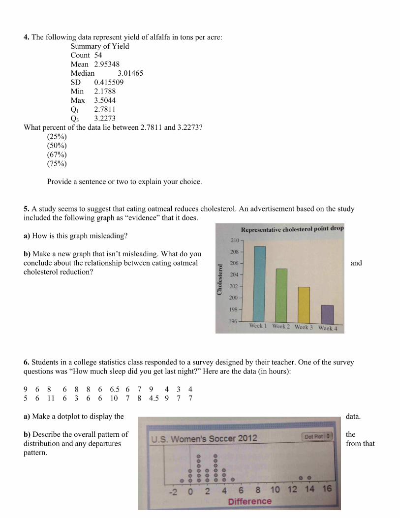
4. The following data represent yield of alfalfa in tons per acre: Summary of Yield Count 54 Mean 2.95348 Median 3.01465 SD 0.415509 Min 2.1788 Max 3.5044 Q1 2.7811 Q3 3.2273 What percent of the data lie between 2.7811 and 3.2273? (25%) (50%) (67%) (75%) Provide a sentence or two to explain your choice. 5. A study seems to suggest that eating oatmeal reduces cholesterol. An advertisement based on the study included the following graph as “evidence” that it does. a) How is this graph misleading? b) Make a new graph that isn’t misleading. What do you conclude about the relationship between eating oatmeal and cholesterol reduction? 6. Students in a college statistics class responded to a survey designed by their teacher. One of the survey questions was “How much sleep did you get last night?” Here are the data (in hours): 9 6 8 6 8 8 6 6.5 6 7 9 4 3 4 5 6 11 6 3 6 6 10 7 8 4.5 9 7 7 a) Make a dotplot to display the data. b) Describe the overall pattern of the distribution and any departures from that pattern.

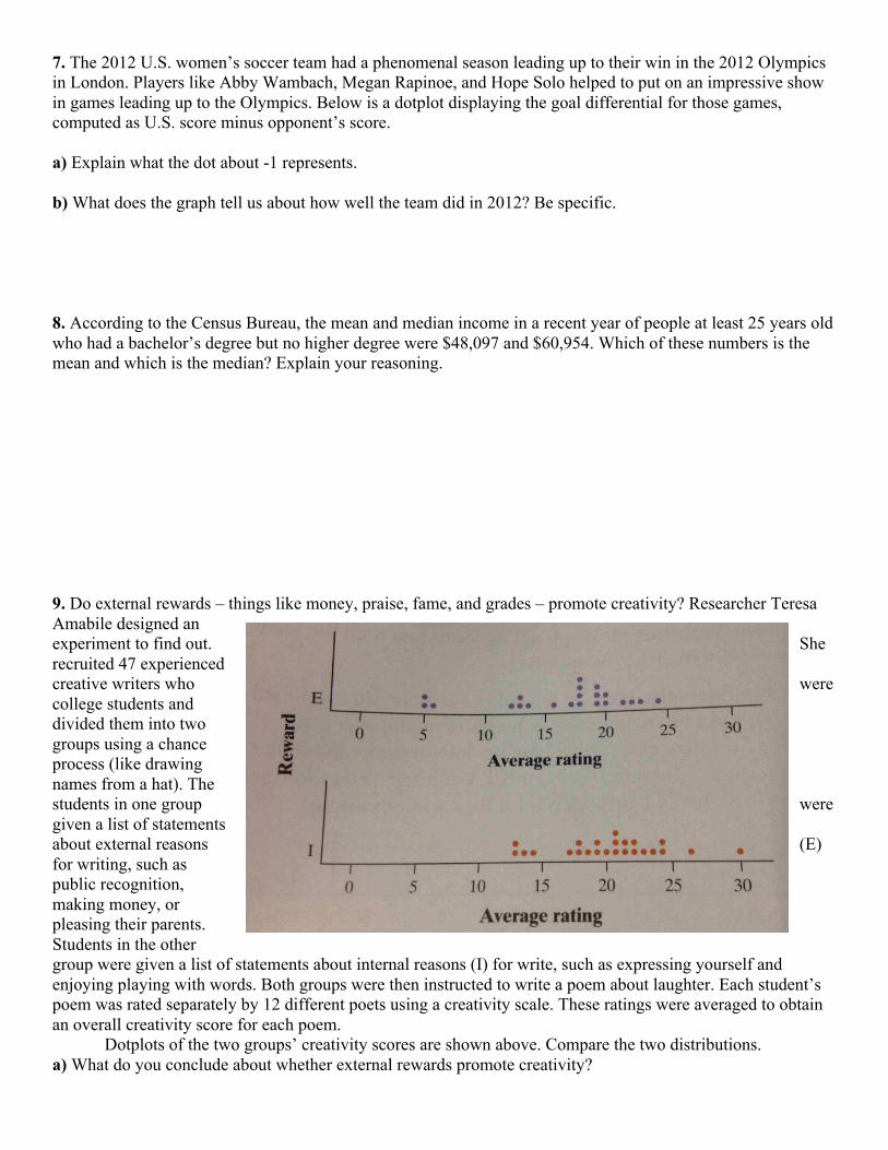
7. The 2012 U.S. women’s soccer team had a phenomenal season leading up to their win in the 2012 Olympics in London. Players like Abby Wambach, Megan Rapinoe, and Hope Solo helped to put on an impressive show in games leading up to the Olympics. Below is a dotplot displaying the goal differential for those games, computed as U.S. score minus opponent’s score. a) Explain what the dot about -1 represents. b) What does the graph tell us about how well the team did in 2012? Be specific. 8. According to the Census Bureau, the mean and median income in a recent year of people at least 25 years old who had a bachelor’s degree but no higher degree were $48,097 and $60,954. Which of these numbers is the mean and which is the median? Explain your reasoning. 9. Do external rewards – things like money, praise, fame, and grades – promote creativity? Researcher Teresa Amabile designed an experiment to find out. She recruited 47 experienced creative writers who were college students and divided them into two groups using a chance process (like drawing names from a hat). The students in one group were given a list of statements about external reasons (E) for writing, such as public recognition, making money, or pleasing their parents. Students in the other group were given a list of statements about internal reasons (I) for write, such as expressing yourself and enjoying playing with words. Both groups were then instructed to write a poem about laughter. Each student’s poem was rated separately by 12 different poets using a creativity scale. These ratings were averaged to obtain an overall creativity score for each poem. Dotplots of the two groups’ creativity scores are shown above. Compare the two distributions. a) What do you conclude about whether external rewards promote creativity?

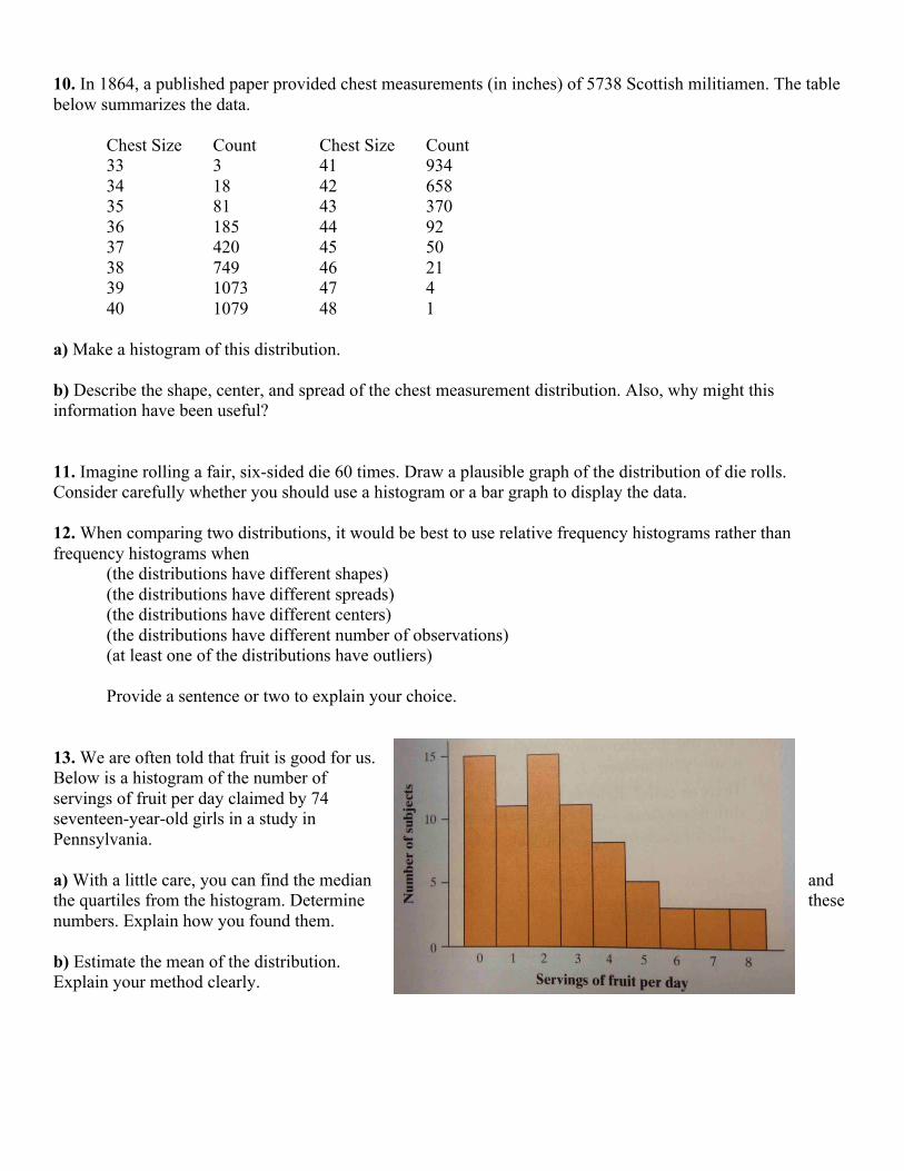
10. In 1864, a published paper provided chest measurements (in inches) of 5738 Scottish militiamen. The table below summarizes the data. Chest Size Count Chest Size Count 33 3 41 934 34 18 42 658 35 81 43 370 36 185 44 92 37 420 45 50 38 749 46 21 39 1073 47 4 40 1079 48 1 a) Make a histogram of this distribution. b) Describe the shape, center, and spread of the chest measurement distribution. Also, why might this information have been useful? 11. Imagine rolling a fair, six-sided die 60 times. Draw a plausible graph of the distribution of die rolls. Consider carefully whether you should use a histogram or a bar graph to display the data. 12. When comparing two distributions, it would be best to use relative frequency histograms rather than frequency histograms when (the distributions have different shapes) (the distributions have different spreads) (the distributions have different centers) (the distributions have different number of observations) (at least one of the distributions have outliers) Provide a sentence or two to explain your choice. 13. We are often told that fruit is good for us. Below is a histogram of the number of servings of fruit per day claimed by 74 seventeen-year-old girls in a study in Pennsylvania. a) With a little care, you can find the median and the quartiles from the histogram. Determine these numbers. Explain how you found them. b) Estimate the mean of the distribution. Explain your method clearly.

14. In a September 28, 2008 article titled “Letting Our Fingers Do the Talking.” the New York Times reported that Americans now send more text messages than they make phone calls. According to a study by Nielsen Mobile, “Teenagers ages 13 to 17 are by far the most prolific texters, sending or receiving 1742 messages a month.” Mr. Williams, a high school statistics teacher, was skeptical about the claims in the article. So he collected data from his first-period statistics class on the number of text messages and calls they had sent or received in the past 24 hours. Here are the texting data. 0 7 1 29 25 8 5 1 25 98 9 0 26 8 118 72 0 92 52 14 3 3 44 5 42 a) Make a boxplot of these data by hand. Be sure to check for outliers. b) Explain how these data seem to contradict the claim in the article. 15. Individuals with low bone density have a high risk of broken bones (fractures). Physicians who are concerned about low bone density (osteoporosis) in patients can refer them for specialized testing. Currently, the most common method for testing bone density is dual-energy X-ray absorptiometry (DEXA). A patient who undergoes a DEXA test usually gets bone density results in grams per square centimeter (g/cm2) and in standardized units. Judy, who is 25 years old, has her bone density measured using DEXA. Her results indicate a bone density in the hip of 948 g/cm2 and a standardized score of z = -1.45. In the reference population of 25-year-old women like Judy, the mean bone density in the dip is 956 g/cm2. a) Judy has not taken a statistics class in a few years. Explain to her in simple language what the standardized score tells her about her bone density. b) Use the information provided to calculate the standard deviation of bone density in the reference population. 16. The scores on Ms. Martin’s English quiz had a mean of 12 and a standard deviation of 3. Ms. Martin wants to transform the scores to have a mean of 75 and a standard deviation of 12. What transformations should she apply to each test score? Explain. 17. An important measure of the performance of a locomotive is its “adhesion,” which is the locomotive’s pulling force as a multiple of its weight. The adhesion of one 4400-horsepower diesel locomotive varies in actual use according to a Normal distribution with mean 37.0=µ and standard deviation 04.0=σ . a) For a certain small train’s daily route, the locomotive needs to have an adhesion of at least 0.30 for the train to arrive at its destination on time. On what proportion of days will this happen? Show your method. b) An adhesion greater than 0.50 for the locomotive will result in a problem because the train will arrive too early at a switch point along the route. On what proportion of days will this happen? Show your method. c) Compare your answers from parts a) and b). What recommendations would you make to the locomotive company about the mean adhesion in order to minimize trains being late as well as minimize trains being early?

18. A species of cockroach has weights that follow a Normal distribution with a mean of 50 grams. After measuring the weights of many of these cockroaches, a lab assistant reports that 14% of the cockroaches weight more than 55 grams. Based on this report, what is the approximate standard deviation of weights for this species of cockroaches? (4.6) (5.0) (6.2) (14.0) (Cannot determine without more information) Provide a sentence or two to explain your choice.