1

AOSC 634Air Sampling and Analysis

Lecture 3Measurement Theory

Performance Characteristics of InstrumentsDynamic Performance of Sensor Systems

Response of a second order system to A step changeA ramp change

Copyright Brock et al. 1984; Dickerson 2015

2

Dynamic ResponseSensor output in response to changing input.

Dynamic Characteristics of Second Order Systems

EQ I

• Where wn is the undamped natural frequency, a constant (s-1).

• z is the damping ratio, a unitless constant. • We must solve an initial value problem.

3

Solving the differential equation

We will use the technique of variation of parameters to find complementary solutions.

We must assume a time dependence of the form ert and substitute this into Eq I.

The characteristic equation is:

Each root gives rise to a solution; there are four.

4

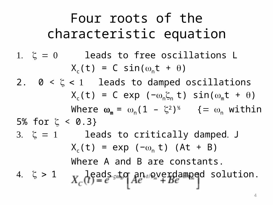
Four roots of the characteristic equation

1. = 0 z leads to free oscillations LXc(t) = C sin(wnt + q)

2. 0 < < 1 z leads to damped oscillationsXc(t) = C exp (−wnzn t) sin(wmt + q)

Where wm = wn(1 – z2)½ {= wn within 5% for z < 0.3}3. = 1 z leads to critically damped. J

Xc(t) = exp (−wn t) (At + B)

Where A and B are constants. 4. > z 1 leads to an overdamped solution.

5

4. > z 1 leads to an overdamped solution.

Where tm = 1/wm

And the characteristic time is 1/wm

In dimensionless time wnt = t”

Critically damped systems are an ideal; in the real world only overdamped and underdamped systems exist. We will focus on underdamped systems such as the dew pointer (or a car with bad shocks). Overdamped systems lead to a “double first order”.

6

Time Response of second order systems.

• Start with a system at rest where both the input and output are zero. X(0) = XI(0) = X0

Their first derivatives are likewise zero at time zero.

We will proceed as with the first order system assuming a step change. Using the dimension- less form.1. z = 0, no damping. X’(t”) = 1 – cos (t”)

7

Time Response of second order systems.

2. 0 < z < 1.0, underdamped.

3. z = 0, critically damped.X’(t”) = 1 – e-t”(t” + 1)

2/121

2/122/12

"

1cos where

"1cos1

1)"('

te

tXt

8

Time Response of second order systems.

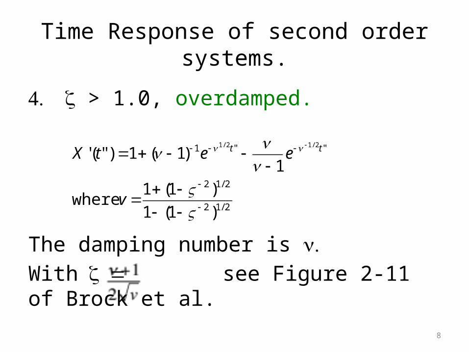
4. z > 1.0, overdamped.

The damping number is .nWith = z see Figure 2-11 of Brock et al.

2/12

2/12

""1

)1(1

)1(1 where

1)1(1)"('

2/12/1

v

eetX tt

9

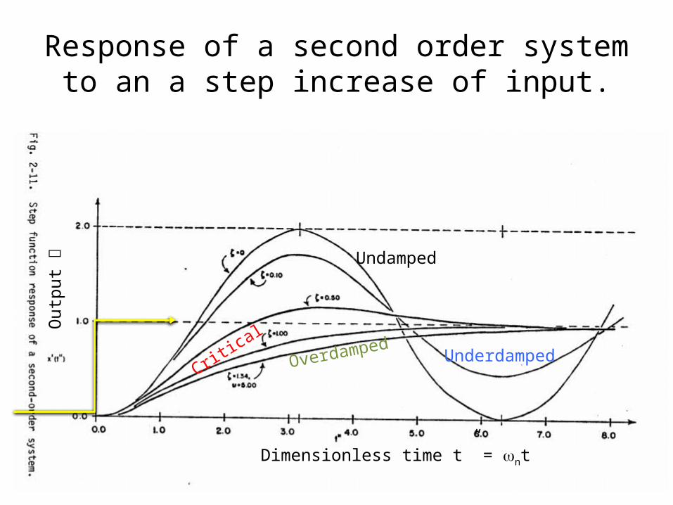
Response of a second order system to an a step increase of input.

Undamped

UnderdampedCriticalOverdamped

Dimensionless time t” = wnt

Out

put

10

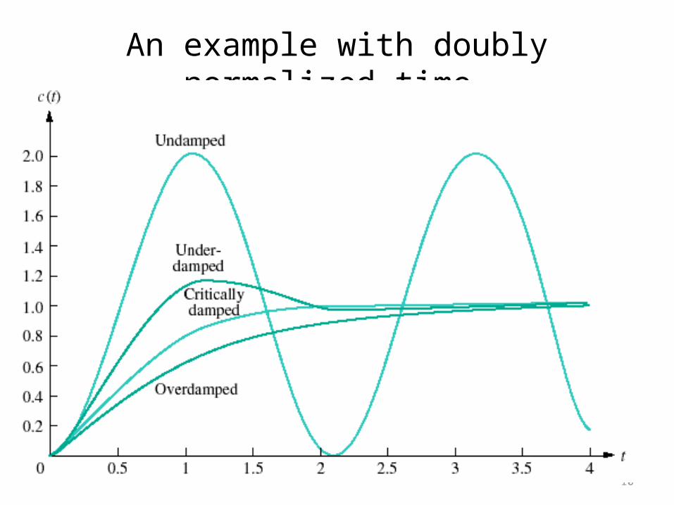
An example with doubly normalized time

11

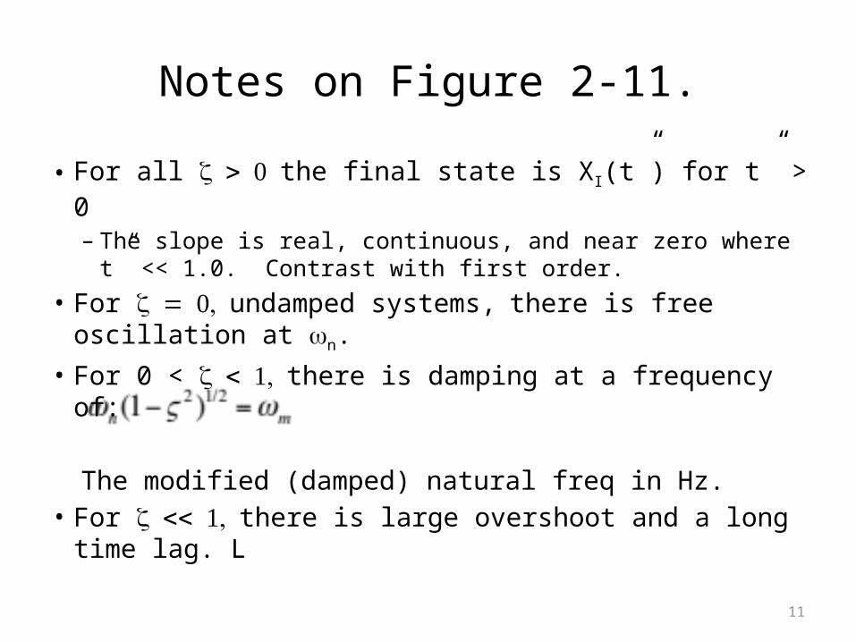
Notes on Figure 2-11.

• For all > 0 z the final state is XI(t”) for t” > 0– The slope is real, continuous, and near zero where t” << 1.0.

Contrast with first order.• For = 0, z undamped systems, there is free oscillation

at wn.• For 0 < < 1, z there is damping at a frequency of:

The modified (damped) natural freq in Hz.• For << 1, z there is large overshoot and a long time

lag. L

12

Notes on Figure 2-11, continued.

• For << 1, z there is large overshoot and a long time lag. L– The amplitude of the oscillations decreases exponentially with a

time constant of z-1.

The extrema can be found:Where the sub e represents

extrema.The extrema come on time at pt”.

Where n is a positive integer.

13

• From the amplitude of the first extreme (assume here a maximum) we can calculate the damping ratio z:

Practical application

14

• From the time (in units of t” of the first extreme (assume here a maximum) we can calculate the natural undamped frequency wn:

15

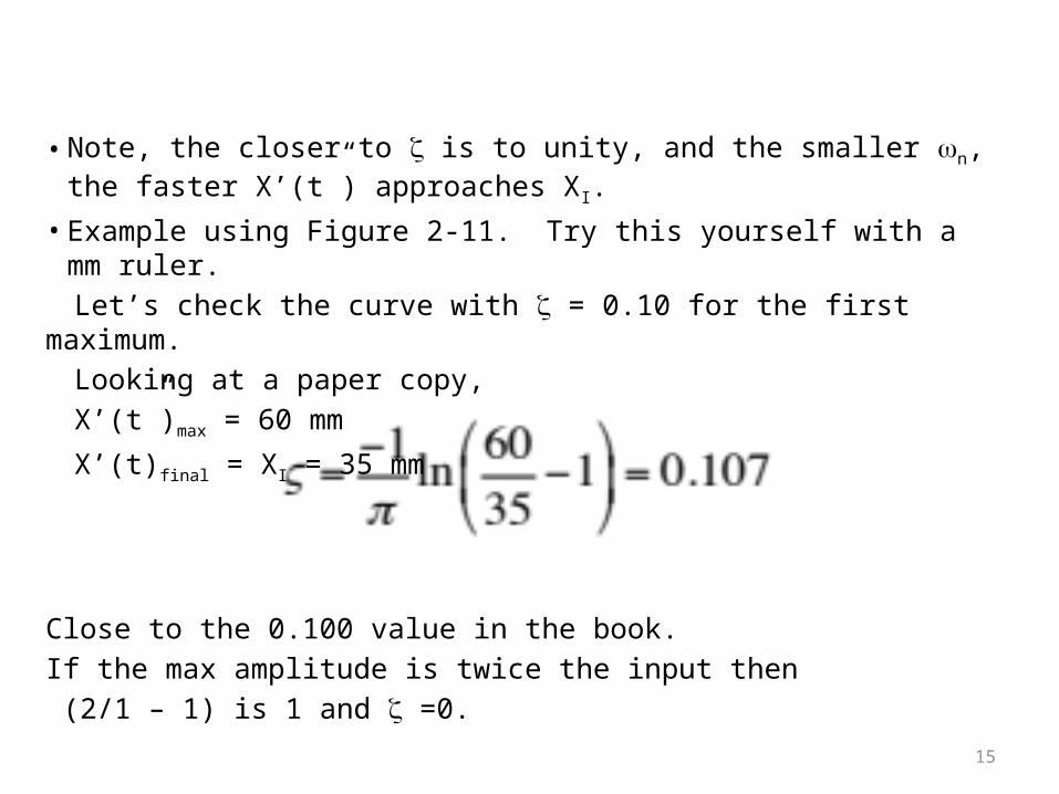
• Note, the closer to z is to unity, and the smaller wn, the faster X’(t”) approaches XI.

• Example using Figure 2-11. Try this yourself with a mm ruler.Let’s check the curve with z = 0.10 for the first maximum. Looking at a paper copy, X’(t”)max = 60 mm

X’(t)final = XI = 35 mm

Close to the 0.100 value in the book. If the max amplitude is twice the input then (2/1 – 1) is 1 and z =0.

16

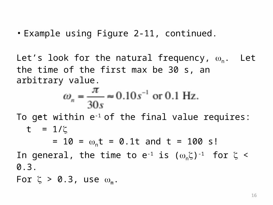
• Example using Figure 2-11, continued.

Let’s look for the natural frequency, wn. Let the time of the first max be 30 s, an arbitrary value.

To get within e-1 of the final value requires:t” = 1/z = 10 = wnt = 0.1t and t = 100 s!

In general, the time to e-1 is (wnz)-1 for z < 0.3.

For z > 0.3, use wm.

17

Summary

• Although less intuitive than first order systems, second order systems lend themselves to analysis of performance characteristics.

• A step change is in some ways a worst case scenario for overshoot. Any second order systems provide perfectly adequate temporal response in the real world where geophysical variables tend to show wave structure.

18

References

• MacCready and Henry, J. Appl Meteor., 1964.• Determination of the Dynamic Response of a

Nitric Oxide Detector, K. L. Civerolo, J. W. Stehr, and R. R. Dickerson, Rev. Sci. Instrum., 70(10), 4078-4080, 1999.