Antoine Deleforge and Radu Horaud

appor t de r ech er ch e

ISS

N02

49-6

399

ISR

NIN

RIA

/RR

--75

29--

FR+E

NG

Domaine 4

INSTITUT NATIONAL DE RECHERCHE EN INFORMATIQUE ET EN AUTOMATIQUE

Learning the Direction of a Sound Source UsingHead Motions and Spectral Features

Antoine Deleforge and Radu Horaud

N° 7529

February 2011

Centre de recherche INRIA Grenoble – Rhône-Alpes655, avenue de l’Europe, 38334 Montbonnot Saint Ismier

Téléphone : +33 4 76 61 52 00 — Télécopie +33 4 76 61 52 52

Learning the Direction of a Sound Source Using HeadMotions and Spectral Features

Antoine Deleforge ∗ and Radu Horaud

Domaine : Perception, cognition, interaction

Equipe-Projet PERCEPTION

Rapport de recherche n° 7529 — February 2011 — 28 pages

Abstract: In this paper we address the problem of localizing a sound-source bycombining binaural or monaural spectral features with head movements. Based ona number of psychophysical and behavioral studies suggesting that the problem ofspatial hearing is both listener-dependent and dynamic, we propose to address theproblem at hand within the framework of unsupervised learning. More precisely, ourmethod is able to retrieve an intrinsic low-dimensional parameterization from the high-dimensional spectral representation of the acoustic input. We address both binauraland monaural spatial localization with both static and dynamic cues. We show that therecovered low-dimensional representations are homeomorphic to the two-dimensionalmanifold associated with the motor states of a robotic head with two rotational degreesof freedom. We describe the experimental setup and protocols allowing us to gatheracoustic data sets with ground truth for both the emitter-to-listener directions and pre-cise head motions. We validate our method using extensive experiments that consistin classifying acoustic vectors from a test set, based on manifold learning with a dif-ferent training set. Our method strongly contrasts with current approaches in soundlocalization because it puts forward the role of learning.

Key-words: Sound source localization, dynamic auditory cues, manifold learning,sensorimotor integration.

This work was supported by the European project HUMAVIPS, under EU grant FP7-ICT-2009-247525.

∗ Corresponding author: [email protected]

Apprendre la Direction d’une Source Sonore enCombinant Mouvements de Tete et Caracteristiques

Spectrales.

Resume : Dans ce papier, nous abordons le probleme de la localization sonore encombinant les caracteristiques spectrales monaurales et binaurales des sons a des mou-vements de tete. Partant de nombreuses observations psychophysiques et comporte-mentales suggerant que le probleme de l’audition spatiale est a la fois dynamique etdependante du sujet, nous proposons d’envisager le probleme par le biais de l’apprentissagenon-supervise. Plus precisement, notre methode permet de retrouver une parametrisationintrinseque en basse dimension a partir d’une representation spectrale en haute dimen-sion des donnees acoustiques. Nous traitons a la fois la localisation binaurale et monau-rale, avec des indices statiques ou dynamiques. Nous montrons que les representationsen basse dimension obtenues sont homeomorphiques a la variete bidimensionelle as-sociee aux etats moteurs d’une tete robotique dotee de deux degrees de libertee ro-tationels. Nous decrivons l’installation et les protocols experimentaux qui nous ontpermis de reunir un ensemble de donnees acoustiques, precisement annotees a la foispar la direction emeteur-recepteur et les mouvements de tetes. Nous validons notremethode par des experiences approffondies consistant a classifier les vecteurs acous-tiques d’un ensemble test, en se servant d’une variete apprise a partir d’un ensem-ble d’entraınement different. Notre methode contraste fortement avec les approchesactuelles en localisation sonore car elle met en avant le role de l’apprentissage.

Mots-cles : Localisation sonore, indice audio dynamique, apprentissage de variete,integration sensori-motrice.

Spectral and Dynamic Sound Source Direction Learning 3

Contents

1 Introduction, Related Work, and Contribution 4

2 Experimental Setup and Data Acquisition 6

2.1 The Experimental Setup . . . . . . . . . . . . . . . . . . . . . . . . 7

2.2 Recording Audio-Motor Contingencies . . . . . . . . . . . . . . . . 7

3 A Computational Model for Audio-motor Localization 9

3.1 The ILD Manifold . . . . . . . . . . . . . . . . . . . . . . . . . . . . 11

3.2 The Dynamic Acoustic Manifold . . . . . . . . . . . . . . . . . . . . 11

4 From Sound Signals to Acoustic Vectors 12

4.1 Spectrograms . . . . . . . . . . . . . . . . . . . . . . . . . . . . . . 12

4.2 Acoustic Input and ILD Vectors . . . . . . . . . . . . . . . . . . . . 15

4.3 Dynamic Acoustic Vectors . . . . . . . . . . . . . . . . . . . . . . . 15

4.4 Content-Independent Spatial Auditory Cues . . . . . . . . . . . . . . 16

5 Manifold Learning Via Dimensionality Reduction 17

6 Computational experiments and results 19

6.1 The Manifold of Acoustic Inputs . . . . . . . . . . . . . . . . . . . . 20

6.2 The ILD Manifold . . . . . . . . . . . . . . . . . . . . . . . . . . . . 21

6.3 The Dynamic Acoustic Manifold . . . . . . . . . . . . . . . . . . . . 21

6.4 Sound Localization and Missing Frequencies . . . . . . . . . . . . . 22

7 Conclusion 25

RR n° 7529

4 Deleforge & Horaud

1 Introduction, Related Work, and Contribution

The humans’ instinctive capability of localizing one or several sound sources from theperceived acoustic signals has been intensively studied in cognitive sciences Blauert(1997). Nevertheless, both the existence and the full understanding of a sound local-ization pathway in the brain are still active topics of research and the exact anatomyand physiology of the auditory cortex is still under debate King and Schnupp (2007).This has also been actively investigated within the framework of computational audi-tory scene analysis (CASA) Wang and Brown (2006). A classical example that illus-trates well the difficulty of the problem is the well known cocktail party problem (CPP)Cherry (1953); Haykin and Chen (2005): How do listeners manage to decipher speechin the presence of other sound sources, including competing talkers? We note that untiltoday this auditory source separation problem has not received yet a fully satisfactoryanswer from both neurophysiological and computational perspectives. We believe thatfinding a proper solution to the problem of three dimensional (3D) sound localizationis key to fully understanding every day situations which are often analogous to the CPP.

There is behavioral and physiological evidence that human listeners use interauraldifferences in order to estimate the direction of a sound. Two binaural cues seem toplay an essential role, namely the interaural level difference (ILD) and the interauraltime difference (ITD). The ITD, measured at the eardrum for broadband stimuli, isapproximately constant in the frequency domain and it depends on sound source ori-entation in approximately the same way from subject to subject. Nevertheless, it is anambiguous sound localization cue since a number of different sound directions couldproduce the same ITD value. Alternatively, the ILD is both subject-dependent andfrequency-dependent. A number of computational models were developed for robustsound localization and sound tracking based on ITD and ILD Willert et al. (2006);Roman and Wang (2008). However, to the extent that both the head and the ears aresymmetric, a stimulus presented at any location on the median plane should produceno interaural differences. Similarly, any point off this median plane falls on a cone ofconfusion Woodworth and Schlosberg (1965), upon which the overall interaural differ-ences, either ILD or ITD, are constant. Therefore, the spatial information provided byinteraural-difference cues, within a restricted band of frequency, is spatially ambigu-ous, particularly along a roughly vertical and front/back dimension Middlebrooks andGreen (1991).

More elaborate sound localization models incorporate the head related transferfunction (HRTF) and the head-related impulse response (HRIR). For example, azimuthestimation can be done by HRTF data lookup. Based on studying the HRIR parame-ters of each individual in a database of 45 subjects, Raspaud et al. (2010) proposes ageneric model for the relationship between azimuth angle and ILDs and ITDs that onlydepends on one parameter (the distance between the ears). Interesting enough, theyexperiment with musical signals which have a more complex time-frequency behav-ior than speech. The idea of HRTF data lookup is also considered in Lu and Cooke(2010) in conjunction with the direct-to-reverberant energy ratio (DRR) that is used tomeasure the distance to a sound source. However, this method can only estimate the

INRIA


listener-to-source distance with an accuracy of 1m for static sources and 1.5-3.5m formoving sources.

So far we considered a static listener. Dynamic cues for sound localization are as-sociated with head movements. Based on behavioral data, it has been hypothesizedsome time ago that head motions might be useful for disambiguating potential con-fusions generated by the pinna’s filter Wallach (1939, 1940). Other psychophysicalexperiments Thurlow and Runge (1967); Fisher and Freedman (1968); Pollack andRose (1967) further support the idea that head movements are useful for localization.From a computational point of view Wenzel (1995) evaluated the theoretical contribu-tion of ITDs and ILDs coupled with head motions; it was found that head movementshelp to solve location confusions considerably. In Muller and Schnitzler (1999a,b,2001), based on an acoustic flow theory and on observations on bats, it is argued thatthe synthesis of dynamic cues, e.g., frequency and amplitude modulations, could allowthe individuals to derive useful temporal cues for sound localization. This was testedin practice Handzel and Krishnaprasad (2002) by placing acoustic sensors in a binau-ral configuration such that a bio-inspired computational model can be derived. It wasshowed that the use of acoustic flow under head rotations helped to break the inherentsymmetry of the binaural system and thus solve for location ambiguities.

In Walker et al. (1998) it is suggested that synthesizing different views (perspec-tives) by repositioning the pinnae could also break those symmetries. Kneip and Bau-mann (2008) applied this concept by gathering ITD values from different motor stateswith a two-microphone device with two degrees of freedom, thus allowing a robot tolocalize static and continuous sound sources in space with a precision of 10◦ and 0.5meters.

More generally, the idea of using deliberate head motions for auditory scene anal-ysis has received little attention from a computational point of view, in spite of psy-chophysical evidence that humans use dynamic cues for sound localization Blauert(1997). Dynamic hearing has recently become an emerging topic in robotics because itenables humanoid robots to localize sounds in order to interact with their environment.One advantage of robots over a static device, is that they can achieve precise goal-directed movements. This can be explored to learn the mapping between sound-sourcelocations and observed acoustic signals for various head movements. This mappingcan be learnt in a supervised manner, using a linear regression function as done inHornstein et al. (2006) or in an unsupervised way using a manifold learning techniqueas done in Aytekin et al. (2008). Indeed, rather than attempting to derive specific mod-els for extracting auditory cues from the acoustic signals, as it has been done in the past,it may be interesting to attempt to learn a parameterization of the spatial informationbeing embedded in the observed data.

In this paper we propose an unsupervised learning method that solves for the sin-gle sound-source direction retrieval problem using either static binaural or dynamicmonaural spectral cues. The HRTF is a function that depends on three parameters forsound sources in the far field Otani et al. (2009): the frequency f of the emitter, theazimuth φ and elevation θ of the line joining the emitter to the listener, i.e., h(f, φ, θ).First we show that the ILDs lie on a smooth two-dimensional (non-linear) manifold

RR n° 7529


embedded in RN , where N is the number of frequency channels used to representsounds, and that the ILD-manifold is independent of the spectrum of the emitter. Sec-ond we consider the time derivatives of the acoustic inputs which will be referred toas dynamic acoustic vectors. These vectors (one for each microphone) may well beviewed as dynamic monaural cues and can be estimated from infinitesimal pan andtilt head motions. We show that although they correspond to the differentiation of asignal in RN , they lie on a smooth two-dimensional manifold. As is the case with theILD-manifold, they are independent of the spectrum of the emitter.

Consequently, the problem of sound-source localization becomes the problem oflearning two-dimensional manifolds for both binaural and monaural cues. An ex-plicit derivation of these continuous manifolds would require an explicit formula forthe HRTF. Instead we propose to sample the manifolds by gathering a large numberof N -dimensional acoustic observations, each such observation being associated witha different head position (parameterized by pan and tilt angles) and with infinitesimalhead motions. Hence the problem of building these manifolds becomes an instanceof the non-linear dimensionality reduction problem. One way to solve the latter is touse manifold learning techniques Belkin and Niyogi (2003); Saul and Roweis (2003);Zhang and Zha (2004). We note that, while manifold learning has extensively beenused in image analysis and in data mining, it has barely been used for sound localiza-tion.

The remainder of this paper is organized as follows. Section 2 describes the ex-perimental setup and the methodology used to gather large training sets of static anddynamic binaural recordings. Section 3 presents a new computational model for audio-motor localization. Section 4 describes in detail techniques used to process collectedsounds into training vector sets. Section 5 describes the non-linear dimensionality re-duction technique used in practice. The results of our experiments are described anddiscussed in section 6. Conclusion and directions for future work are presented insection 7.

2 Experimental Setup and Data Acquisition

Existing auditory databases mainly deal with static listeners/emitters. Therefore, oneof our first concerns has been to record sounds in the presence of head motions andfor various emitter-to-listener directions. We believe that collecting such a large dataset of monaural/binaural recording with its associated ground-truth is a contributionin its own right 1. We opted to place a dummy head onto a robot that can performfast, silent, and accurate movements with several degrees of freedom. Moreover, theexperiments were carried out in real-world conditions, i.e., a room with reverberationsand background noise.

1All our recordings with associated parameters and ground truth were made publicly available online athttp://perception.inrialpes.fr/˜Deleforge/CAMIL_Dataset.

INRIA


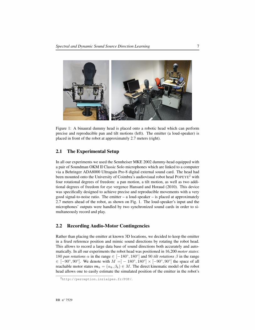
Figure 1: A binaural dummy head is placed onto a robotic head which can performprecise and reproducible pan and tilt motions (left). The emitter (a loud-speaker) isplaced in front of the robot at approximately 2.7 meters (right).

2.1 The Experimental Setup

In all our experiments we used the Sennheiser MKE 2002 dummy-head equipped witha pair of Soundman OKM II Classic Solo microphones which are linked to a computervia a Behringer ADA8000 Ultragain Pro-8 digital external sound card. The head hadbeen mounted onto the University of Coimbra’s audiovisual robot head POPEYE2 withfour rotational degrees of freedom: a pan motion, a tilt motion, as well as two addi-tional degrees of freedom for eye vergence Hansard and Horaud (2010). This devicewas specifically designed to achieve precise and reproducible movements with a verygood signal-to-noise ratio. The emitter – a loud-speaker – is placed at approximately2.7 meters ahead of the robot, as shown on Fig. 1. The loud-speaker’s input and themicrophones’ outputs were handled by two synchronized sound cards in order to si-multaneously record and play.

2.2 Recording Audio-Motor Contingencies

Rather than placing the emitter at known 3D locations, we decided to keep the emitterin a fixed reference position and mimic sound directions by rotating the robot head.This allows to record a large data base of sound directions both accurately and auto-matically. In all our experiments the robot head was positioned in 16,200 motor states:180 pan rotations α in the range ∈ [−180◦, 180◦] and 90 tilt rotations β in the range∈ [−90◦, 90◦]. We denote with M =] − 180◦, 180◦] × [−90◦, 90◦] the space of allreachable motor states mk = (αk, βk) ∈ M . The direct kinematic model of the robothead allows one to easily estimate the simulated position of the emitter in the robot’s

2http://perception.inrialpes.fr/POP/.

RR n° 7529


frame as a function of pan and tilt: xsyszs

=

cosβ cosα − sinα cosα sinβcosβ sinα cosα sinα sinβ

sinβ 0 cosβ

d0r

+ r

cosα sinβsinα sinβ

cosβ

(1)

Notice that this model needs only two parameters: the distance from the tilt-axis to themicrophones’ midpoint, r = 0.22m, and the distance from this midpoint to the emitter,d = 2.70m. Indeed, the robot was designed such that the pan-axis passes through themicrophones’ midpoint.

It is straightforward to notice that while the space M , spanned by (α, β) pairs hasa cylindrical topology (a ruled surface homeomorphic to a plane), the space of all pos-sible sound-source positions (xs, ys, zs) approximately lies on a sphere. One can alsoeasily see that several distinct motor states can correspond to the same sound-sourceposition. Therefore, the two spaces have different topologies and are not isomorphic,which means that there is an intrinsic difference between sampling the motor statespace – as done in our case – and the sound-source position space.

In addition, with this approach, a recording made at a given motor-state only ap-proximates the sound that would actually be perceived if the source was moved to thecorresponding relative position in the room. First, the room moves together with theloud-speaker in the robot’s frame, which modifies perceived reverberations. Second,the mechanical set up used implies that pan movements induce different sound sourcedisplacements in the robot frame depending on the current tilt position. The last ap-proximation will raise issues that are further discussed in Section 6.3.

For each motor state mk ∈ M , we perform both static and dynamic binauralrecordings of artificial reference and random-spectrum sounds emitted by the loud-speaker, as summarized in Table 1. An emitted sound corresponds to:

l(t) = K

N∑i=1

ωi sin(2πfit+ φi) t ∈ [0, 1] (2)

where l(t) is the loud-speaker’s membrane displacement as a function of time t,K ∈ Ris the global volume, F = {f1 . . . fi . . . fN} is a fixed set of N frequency channels,{ωi}i=1..N ∈]0, 1]N and {φi}i=1..N ∈ [0, 2π]N are weights and phases associatedwith each frequency channel. In practice, a set of N = 600 frequency channelsF = {50, 150, 250 . . . , 5950} was used. In order to evaluate the influence of the con-tent of emitted sounds, we recorded both a reference sound, i.e., ωi and φi are fixed forall motor states, and random-spectrum sounds, i.e., ωi and φi are drawn from a uniformdistribution at each motor state. We used these sounds because of two interesting prop-erties of their spectrograms. First they are rich (many frequency channels represented)which makes them likely to contain rich spatial information. Second they are steady(constant energy at each frequency channel in time) which is crucial to measure the real

INRIA


influence of head movements on perceived sounds. At each motor state mk we per-formed the following recordings with both the reference sound and a random-spectrumsound (each such recording lasts one second):

• A binaural recording with a static listener

• A binaural recording while the listener performs a pan rotation with a constantangular velocity α = 9◦/s

• A binaural recording while the listener performs a tilt rotation with a constantangular velocity β = 9◦/s

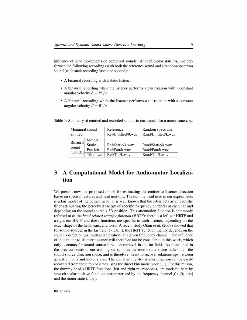
Table 1: Summary of emitted and recorded sounds in our dataset for a motor statemk.

Monaural sound Reference Random spectrumemitted Ref/Emitted/0.wav Rand/Emitted/k.wav

Binauralsoundrecorded

MotorsStatic Ref/Static/k.wav Rand/Static/k.wavPan left Ref/Pan/k.wav Rand/Pan/k.wavTilt down Ref/Tilt/k.wav Rand/Tilt/k.wav

3 A Computational Model for Audio-motor Localiza-tion

We present now the proposed model for estimating the emitter-to-listener directionbased on spectral features and head motions. The dummy head used in our experimentsis a fair model of the human head. It is well known that the latter acts as an acousticfilter attenuating the perceived energy of specific frequency channels at each ear anddepending on the sound source’s 3D position. This attenuation function is commonlyreferred to as the head related transfer function (HRTF): there is a left-ear HRTF anda right-ear HRTF and these functions are specific to each listener, depending on theexact shape of the head, ears, and torso. A recent study Otani et al. (2009) showed thatfor sound-sources in the far field (> 1.8m), the HRTF function mainly depends on thesource’s direction (azimuth and elevation) at a given frequency channel. The influenceof the emitter-to-listener distance will therefore not be considered in this work, whichonly accounts for sound source direction retrieval in the far field. As mentioned inthe previous section, our training-set samples the motor-state space rather than thesound-source direction space, and is therefore meant to recover relationships betweenacoustic inputs and motor states. The actual emitter-to-listener direction can be easilyrecovered from these motor states using the direct kinematic model (1). For this reason,the dummy head’s HRTF functions (left and right microphones) are modeled here bysmooth scalar positive functions parameterized by the frequency channel f ∈]0; +∞[and the motor state (α, β):

RR n° 7529


h : ]0; +∞[×M −→ ]0; +∞[hL : (f, α, β) 7−→ hL(f, α, β)hR : (f, α, β) 7−→ hR(f, α, β)

(3)

The smoothness assumption of the HRTF will be validated using experimentaldata in Section 4.2. Given an arbitrarily large set of N frequency channels F ={f1 . . . fi . . . fN} we approximately represent a sound with an N -dimensional fre-quency vector x = (x1 . . . xi . . . xN )T ∈ [0,+∞[N , where the i-th element xi cor-responds to the mean intensity of the sound at frequency channel fi, during a fixedtemporal integration window. The way such vectors can be computed in practice fromraw sound signals will be detailed in Section 4. With these notations, xE refers toan emitted sound while xL and xR refer to sounds recorded by the robot’s left andright ears. For a motor-state (α, β) ∈ M , the HRTF model leads to the followingrelationship between emitted and recorded sounds:{

xLi = hL(fi, α, β)xEi ∀i ∈ [1;N ]xRi = hR(fi, α, β)xEi ∀i ∈ [1;N ] (4)

We will use the term energy to refer to the logarithm of a given frequency channel’sintensity. We then define an acoustic input vector which corresponds to the perceivedenergy at each frequency channel:

s = logx ∈ RN (5)

We will use the notations sL and sR to denote the acoustic input vectors at the leftand right ears, as well as sL,R = (sL, sR) ∈ R2N to denote their concatenation. Notethat this definition is only valid to the extent that xi > 0 ∀i ∈ [1;N ], that is, if allthe frequency channels are represented in the emitted and perceived sounds, which wasalways the case with the recordings described in Section 2 thanks to the specific waysounds were generated (i.e. (2). This is a relatively strong assumption since most ofthe real world sounds do not have a full spectrum. However, the present model onlyapplies to these recordings, and we will explain in Section 6.4 how they can then beused as training data in order to retrieve the direction of unknown acoustic observationseven with a fair amount of missing frequency channels.

By combining (4) and (5) we obtain that ∀i ∈ [1;N ]:

sLi = log hL(fi, α, β) + log xEisRi = log hR(fi, α, β) + log xEi

(6)

Therefore, s is a multi-valued function that maps the motor-state space M and theemitted sound space ]0; +∞[N onto the set S of all possible acoustic input vectors,S ⊂ RN . For a given emitted sound xE , we now consider the set of all possibleacoustic input vectors while the robot is allowed to move in all its motor states:

SxE = {s(xE , α, β) | (α, β) ∈M} (7)

INRIA


Under the assumptions that s is a homeomorphism of motor state parameters fora fixed emitted sound, this set lies on a two-dimensional smooth manifold embeddedin RN and parameterized by (α, β) (cylindrical topology). The existence of such ahomeomorphism between SxE and M will be experimentally validated in Section 6.For an emitted sound xE , we denote by SLxE and SRxE the left and right acoustic inputmanifolds. We also denote by SL,RxE the concatenated acoustic input manifold.

Notice however, that there are as many such manifolds as frequency vectors xE

emitted by the loud-speaker. Learning the structure of such manifolds from acousticinput vectors will only allow to parameterize directions associated with a specific emit-ted sound, which is of limited interest for sound localization. For this reason we willconsider auditory representations that are independent of the emitter’s content xE .

3.1 The ILD Manifold

We define ILD vectors by sILD = sL − sR. For a motor state (α, β) ∈ M and anemitted sound xE ∈]0; +∞[, it is straight-forward to see from 6 that ∀i ∈ [1;N ]:

sILDi = log hL(fi, α, β)− log hR(fi, α, β)= log hILD(fi, α, β) (8)

Since the emitted sound component xEi cancels out, the ILD vectors do not depend onthe sound source content. The ILD space corresponding to the set of all ILD vectorsfrom all emitted sounds and all motor states can therefore be written:

SILD = {sILD(α, β) | (α, β) ∈M} (9)

Under the assumption that sILD is a homeomorphism of motor state parameters,this set lies on a two-dimensional smooth manifold, the ILD manifold, embedded inRN , parameterized by (α, β), and independent of the emitted sound. The existenceof such a homeomorphism between SILD and M will be experimentally validatedin Section 6. Therefore, the ILD vectors sILD ∈ RN may be viewed as content-independent auditory cues for sound localization.

3.2 The Dynamic Acoustic Manifold

So far we considered the static case, i.e., the listener is in a static motor state m =(α, β) while emitted sounds are recorded. We consider now the case of a dynamiclistener. More precisely, we define a motor command c by a tuple (α, β), where αand β correspond to constant angular velocities transmitted to pan and tilt motors. Inparticular, we will later denote:

{cα = (α, 0)cβ = (0, β)

(10)

RR n° 7529


the motor commands corresponding to pan and tilt head movements at constantvelocity, where α = β = 9◦/s.

An infinitesimal motor displacement dm = (dα, dβ) during dt corresponds to atangent vector on the smooth manifold SxE of acoustic inputs. If the robot performsany motor command c from the motor state (α, β) in front of a static and steady sound-source emitting xE , it is therefore natural to study the structure of the acoustic inputvector’s time derivative:

τ (c) =ds

dt(11)

This vector will be referred to as a c-dynamic acoustic vector. Taking the timederivative of (6) under the smoothness assumption of the HRTF we obtain:

τi =dsidt

=∂si∂α

dα

dt+∂si∂β

dβ

dt

=∂ log h(fi, α, β) + log xEi

∂α

dα

dt

+∂ log h(fi, α, β) + log xEi

∂β

dβ

dt

If we define hi = h(fi, α, β) and dhi/dm the gradient of hi at m = (α, β), thiscan be written in a more compact way as:

τi =1hi

(dhidm

)>m (12)

where we used the fact that d log(xEi )/dα = d log(xEi )/dβ = 0. Since the emittedsound component xEi cancels out, the dynamic acoustic vectors do not depend on thesound source’s content. The dynamic acoustic space T (c) corresponding to all dy-namic acoustic vectors obtained for a given motor command c, all emitted sounds, andall motor states is then defined by

T = {τ (α, β) | (α, β) ∈M} (13)

Under the assumption that τ is a homeomorphism of motor state parameters, T (c)constitutes a two-dimensional smooth manifold, the c-dynamic acoustic manifolds, em-bedded in RN , parameterized by (α, β), and independent of the emitted sound. Theexistence of such a homeomorphism between T (c) and M will be experimentally val-idated in Section 6. As previously, there will be left- and right-microphone dynamicacoustic manifolds T (c)L and T (c)R, as well as the concatenated dynamic acousticmanifold T (c)L,R ⊂ RN .

INRIA


4 From Sound Signals to Acoustic Vectors

We now describe the methodology that we use to process raw sound signals collectedduring experiment, i.e, section 2, and to transform these signals into the acoustic inputvectors (6), the ILD vectors (8) and the dynamic acoustic vectors (12).

4.1 Spectrograms

The model described in section 3 requires to represent sounds both in the time andfrequency domains. A commonly used representation in CASA is to use gamma-tonefilter banks Wang and Brown (2006). Although these filters are known to model thehuman auditory system quite well, they also generate overlaps in the intensities of fre-quency channels that are unwished in the framework of our approach. For this reason,we chose to employ simpler spectrograms. These spectrograms are computed using asliding discrete Fourrier transform of the raw signal within a specified time window, inorder to capture the temporal variation of the sound spectrum: They discretize signalsboth in time and frequency. The way this discretization is achieved is critical and mustbe carefully tuned.

Two crucial parameters are to be considered for temporal discretization: the tem-poral integration and the frame shift. The temporal integration is the length of the timewindow inside which the discrete Fourrier transform is computed. For the Fourriertransform to be meaningful, the temporal integration should be at least twice largerthan the largest sound period considered. On the other hand, the notion of instanta-neous frequency will be lost for too large time windows if the sound varies too much.The frame shift parameter corresponds to the delay between two time windows. Thesmaller the frame shift, the higher the resolution of the spectrogram in time, at the costof a higher computational burden.

The discretization of spectrograms in the frequency domain mainly relies on threeparameters: the lowest and highest frequency channels, and the number of channels.One can choose to spread frequency channels within this range either linearly or log-arithmically. In practice, a logarithmic scale should be preferred because it accountsbetter for harmonics generated by the discrete Fourrier transform, and it coincides withthe neural encoding of frequency channels in the human auditory system. There areseveral ways to compute intensity values at a given frequency channel, the simplestone being to average the signal in the frequency domain within a neighboring window.However, experiments showed that using the maximal intensity inside each windowyields more stable spectrograms, by dealing with small frequency fluctuations due tothe sampling approximation or possible Doppler effect.

A good tradeoff between computational cost and spectrogram precision is achievewith a temporal integration of 200ms and a frame shift of 10ms. Fig. 2(a) and (b)show some time-energy curves (logarithm of the spectrogram intensity values at a givenfrequency channel) obtained with these parameters while performing a 180 degrees pan

RR n° 7529


-90 -70 -50 -30 -10 10 30 50 70 90-1

0

1

2

3

4

Pan angle (degrees)

En

erg

y a

t le

ft e

ar

(arb

itra

ry u

nit)

500 Hz

1000 Hz

1500 Hz

2000 Hz

3000 Hz

4000 Hz

5000 Hz

6000 Hz

(a) Time-energy curves for an emitted random sound

-90 -70 -50 -30 -10 10 30 50 70 90-1

0

1

2

3

4

Pan angle (degrees)

En

erg

y a

t le

ft e

ar

(arb

itra

ry u

nit)

500 Hz

1000 Hz

1500 Hz

2000 Hz

3000 Hz

4000 Hz

5000 Hz

6000 Hz

(b) Time-energy curves for another emitted random sound

Figure 2: This figure shows the variation of the energy perceived by the left microphonefor various frequency channels while the static loud-speaker emits two different randomsounds, e.g, (a) and (b), and while the listener performs a 180◦ rotation from left to rightat constant velocity cα in (10).

movement leftwards at constant velocity, i.e, cα in (10), in the presence of a static loud-speaker that emits two distinct random spectrum sounds as defined in (2). These curvescall for several remarks.

First, time-energy curves corresponding to the lowest frequency channels (500 Hz,1000 Hz and 1500 Hz) do not exhibit any coherent variation with respect to the pan

INRIA


angle, they are highly discontinuous and they are not invariant to the emitted sound.This can be explained by the fact that the acoustic filter of the dummy-head only actson sounds with wavelength below the head diameter (≈ 18cm), which correspondsto frequency channels higher than 1900 Hz. This correlates well with numerous psy-chophysical and behavioral observations suggesting that the ILD is mainly responsiblefor sound localization in the high frequency domain, whereas the ITD is rather used forthe low frequency domain Middlebrooks and Green (1991).

Second, time-energy curves above 2000 Hz are invariant with respect to the emittedrandom sound, up to an additive constant, independently of their own and other chan-nel’s energy. This shows that perceived energies of frequency channels are independentfrom each other and only depend on the motor-state parameter α up to an additive con-stant. This may account for an experimental validation of the HRTF acoustic model(3) as well as (6), (8) and (12). Moreover and despite a slight noise, they appear tobe generally continuous and differentiable with respect to the motor-state parameter:This comforts the assumption that the HRTF is a smooth function of the motor-stateparameters, i.e., section 3. Based on these observations, we used the following settingsin order to compute the ILD and dynamic acoustic vectors: There are N = 400 fre-quency channels ranging from 2000 Hz to 6000 Hz in logarithmic scale with a temporalintegration of 200 ms and a frame shift of 10 ms.

Finally, it is worthwhile to notice from Fig. 2 that there are peaks and notches of theHRTF at specific frequencies and angles. These extrema are well known and commonlyreferred to as spectral features in the psycho-acoustical literature. Several experimentson human subjects suggest that they are involved in vertical sound localization (e.g.Hebrank and Wright (1974), Greff and Katz (2007)). In our case, the existence ofsuch extrema corresponds to important local distortions in the studied manifold, whichimplies the need of a relatively dense sampling of the motor-state space (2-3 degreesbetween two adjacent points) for manifold learning to work well in practice. The com-plex shape of the curves also justifies the use of non-linear dimensionality reductiontechniques rather than linear methods.

4.2 Acoustic Input and ILD Vectors

Using the temporal and spectral parameters just mentioned, records which are onesecond long, static and monaural will result in a spectrogram of 81 frequency vectors,each such vector corresponding to N = 400 frequency channels. As shown in the leftplot of Fig. 3, the perceived energy, when the head remains static, is relatively stable intime. This energy is averaged over a period of one second to obtain the N -dimensionalacoustic input vectors sL, sR as well as the ILD vector sILD = sL − sR, e.g., (6) and(8).

4.3 Dynamic Acoustic Vectors

When the listener performs head motions, one is faced with the problem of dynamicrecording in order to estimate the time derivative of the acoustic vectors, namely the

RR n° 7529


0 0.5 11

1.5

2

2.5

3

Time (s)

En

erg

y a

t le

ft e

ar

(arb

itra

ry u

nit)

0 0.5 1

Time (s)

0 0.5 1

Time (s)

2000 Hz

2500 Hz

3000 Hz

3500 Hz

4000 Hz

4500 Hz

5000 Hz

Figure 3: This figure shows the variation of the energy perceived at the left ear, duringone second, and for various frequency channels when a random-spectrum sound xE

is emitted, i.e., (2). Circles represent recorded energy values. Lines correspond toleast-square error linear interpolations of the energy variation. The figure illustratesthe following situations: The head is static (left), the head performs a motor commandcα (middle), and finally the head performs motor command cβ (right).

dynamic acoustic vectors τ (c) (12). As previously, we compute the spectrograms andwe take the logarithm thus yielding N = 400 time-energy curves associated with eachrecording. Fig. 3-middle and -right show that this leads to a significant variation overtime of the perceived energy, at each frequency channel. We used linear regression tolocally approximate this temporal variation:{

sLi (t) = aLi t+ bLisRi (t) = aRi t+ bRi

(14)

where aLi and aRi are the local slopes of the perceived energies sLi and sRi at frequencyfi. We finally define dynamic acoustic vectors using the slopes of these local linearapproximations:

τL(c) = (aL1 . . . aLi . . . a

LN ) (15)

τR(c) = (aR1 . . . aRi . . . a

RN ) (16)

4.4 Content-Independent Spatial Auditory Cues

A preliminary experiment was performed aimed at the validation of the assumptionsthat the ILD vectors and the dynamic acoustic vectors are both invariant with respect

INRIA


to the emitted sound’s spectrum. For that purpose we recorded sounds emitted by astatic loud-speaker while the listener was undergoing a complete 180◦ pan rotation in90 steps of 2◦ each, i.e., 90 pan positions α ∈ [−90◦,+90◦]. At each one of these panpositions we recorded 30 random-spectrum sounds, both with a static and a dynamiclistener, as explained in Section 2.2. This resulted in the computation of 2700 = 90×30left-ear and right-ear acoustic input vectors sL and sR, as well as an equal number ofconcatenated acoustic input vectors sL,R, ILD vectors sILD, and left- and right- cα-dynamic acoustic vectors τL(cα) and τR(cα)10.

(a) Acoustic input vectors sL,R (b) ILD vectors sILD

(c) left-ear cα-dynamic acoustic vectors τL(cα) (d) right-ear cα-dynamic acoustic vectorsτR(cα)

Figure 4: This figure shows 2700×2700 pairwise Euclidean distance matrices betweenvectors obtained at 90 different motor states (90 pan values α ∈ [−90◦,+90◦]) andwith a loud-speaker emitting 30 different random spectrum sounds, i.e., (2). Vectorsare sorted left-right and bottom-down with respect to their corresponding pan value.The distance varies from zero (dark blue) to higher values (dark red) [This figure isbest seen in color].

RR n° 7529


We computed the pairwise distances between these vectors. As it may be seen inFig. 4-(a), the acoustic input vectors sL,R are highly content-dependent and they cannotprovide proper sound localization information. Alternatively, the zero-distance stripearound the 2700 × 2700 matrices’ diagonals in Fig. 4-(b), -(c) and -(d) show that theILD and acoustic dynamic vectors are well suited for sound localization. Indeed, thesezero-distance diagonal stripes correspond to pairwise distances between vectors that areassociated with similar motor states: This validates experimentally the computationalmodel outlined in Section 3.

5 Manifold Learning Via Dimensionality Reduction

The experimental setup (Section 2) and associated sound processing techniques (Sec-tion 4) allow to collect large sets of high-dimensional spectral-feature vectors withground-truth spatial localization. In principle, although these feature vectors are com-puted in a high-dimensional space, they should lie on low-dimensional manifolds thatare parameterized by motor-state parameters. In the absence of an explicit model, wepropose to recover a low-dimensional manifold parameterization through a dimension-ality reduction technique.

If this manifold corresponds to a low-dimensional linear subspace of the high-dimensional spectral-feature vector space, linear methods such as principal compo-nent analysis, or one of its numerous variants, can be used. Nevertheless, the modeldeveloped in Section 3 postulates that the sought manifolds are nonlinear. Severalmanifold learning algorithms have been recently developed, most notably includingkernel PCA Scholkopf et al. (1998), ISOMAP Tenenbaum et al. (2000), local-linearembedding (LLE) Saul and Roweis (2003), or Laplacian eigenmaps (LE) Belkin andNiyogi (2003). Both kernel PCA and ISOMAP can be viewed as generalizations ofmultidimensional scaling (MDS) Cox and Cox (1994) and are based on computing thetop eigenvalues and eigenvectors of a Gram matrix. They require the computation ofeither all the pairwise geodesic distances Tenenbaum et al. (2000) or of all the pairwisekernel dot-products, which may be computationally expensive. Alternatively, methodslike LLE and LE only require the computation of pairwise similarities between eachvector and its neighbors. For large data sets, such as ours, this results in very sparsematrix solvers.

In spite of the elegancy of such methods as LLE and LE, which are widely usedin machine learning applications, we preferred to use the local tangent space align-ment method (LTSA) proposed in Zhang and Zha (2004). This method approximatelyrepresents the data in a lower dimensional space by minimizing a reconstruction errorin 3 steps. First, a local neighborhood around each point is computed. Second, foreach such point, local coordinates of its neighboring points on the local tangent spaceare approximated using PCA. Third, these local coordinates are optimally aligned toconstruct a global low-dimensional representation of the points lying on the manifold.As already noticed in Aytekin et al. (2008), the main advantage of LTSA over spec-tral graph methods, is its ability to work well with non-compact manifold subsets with

INRIA


boundaries, such as is the case with our data. LTSA’s only free parameter is the integerk corresponding to the neighborhood size around each point. We experimented withdifferent values of k and we noticed that, in our case, e.g, 16,200 vectors of dimen-sion 400, the choice of k was not critical. In practice we implemented a fast versionof the kNN algorithm which, in conjunction with sparse matrix solvers, allowed us toimplement an efficient non-linear dimensionality reduction method based on LTSA.

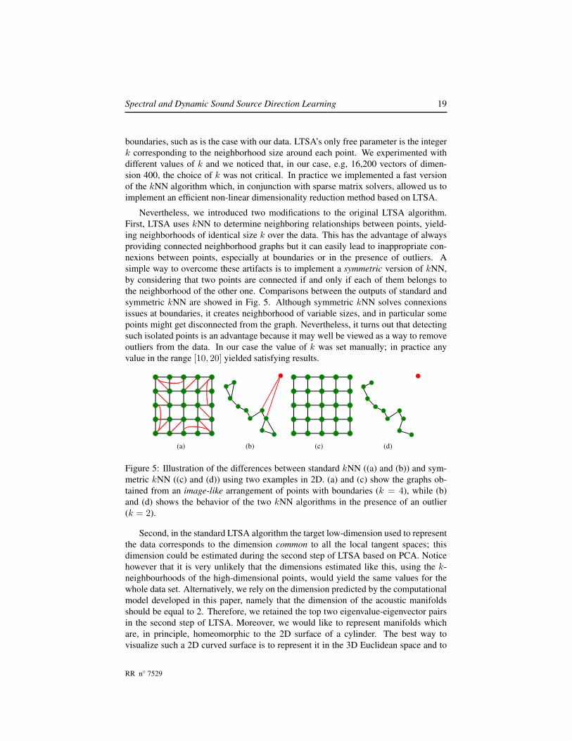
Nevertheless, we introduced two modifications to the original LTSA algorithm.First, LTSA uses kNN to determine neighboring relationships between points, yield-ing neighborhoods of identical size k over the data. This has the advantage of alwaysproviding connected neighborhood graphs but it can easily lead to inappropriate con-nexions between points, especially at boundaries or in the presence of outliers. Asimple way to overcome these artifacts is to implement a symmetric version of kNN,by considering that two points are connected if and only if each of them belongs tothe neighborhood of the other one. Comparisons between the outputs of standard andsymmetric kNN are showed in Fig. 5. Although symmetric kNN solves connexionsissues at boundaries, it creates neighborhood of variable sizes, and in particular somepoints might get disconnected from the graph. Nevertheless, it turns out that detectingsuch isolated points is an advantage because it may well be viewed as a way to removeoutliers from the data. In our case the value of k was set manually; in practice anyvalue in the range [10, 20] yielded satisfying results.

(a) (b) (c) (d)

Figure 5: Illustration of the differences between standard kNN ((a) and (b)) and sym-metric kNN ((c) and (d)) using two examples in 2D. (a) and (c) show the graphs ob-tained from an image-like arrangement of points with boundaries (k = 4), while (b)and (d) shows the behavior of the two kNN algorithms in the presence of an outlier(k = 2).

Second, in the standard LTSA algorithm the target low-dimension used to representthe data corresponds to the dimension common to all the local tangent spaces; thisdimension could be estimated during the second step of LTSA based on PCA. Noticehowever that it is very unlikely that the dimensions estimated like this, using the k-neighbourhoods of the high-dimensional points, would yield the same values for thewhole data set. Alternatively, we rely on the dimension predicted by the computationalmodel developed in this paper, namely that the dimension of the acoustic manifoldsshould be equal to 2. Therefore, we retained the top two eigenvalue-eigenvector pairsin the second step of LTSA. Moreover, we would like to represent manifolds whichare, in principle, homeomorphic to the 2D surface of a cylinder. The best way tovisualize such a 2D curved surface is to represent it in the 3D Euclidean space and to

RR n° 7529


visualize the 3D points lying on that surface. For this reason, we retain the three largesteigenvalue-eigenvector pairs in the global alignment stage of LTSA (third step), suchthat the extracted manifolds can be easily visualized.

6 Computational experiments and results

The method presented above allows to build two-dimensional acoustic manifolds in acompletely unsupervised way and to obtain an intrinsic parameterization, e.g, usingLTSA. Indeed, our computational model predicts that these manifolds are homeomor-phic to the surface of a cylinder parameterized by the motor-state variables (α, β). Thismeans in practice that each manifold point corresponds to an emitter-to-listener sounddirection. However, rather than representing these directions in the extrinsic 3D worldspace, it is represented intrinsically on one of the acoustic manifolds. Once such a man-ifold has been learned, it can be used as a training data set in a classification frameworkto find the direction of a sound emitted from an unknown position.

The experimental setup and data collection protocols described in Section 2 al-lows us to establish a one-to-one association between the manifolds extracted from theacoustic data with LTSA and the ground-truth motor-state values. We will refer to suchan association as an audio-motor map. An audio-motor map proves the existence of ahomeomorphism between the motor-state space and an acoustic manifold (i.e. Section3) if the following three criteria are verified:

• The map has the same topology as the motor-state space (i.e. cylindrical)

• Level-set lines associated with the intrinsic (α, β) manifold parameterizationshould not cross each other

• The ordering of the points along a level-set line must be the same for the acousticand ground-truth manifolds

We implemented a simple method to represent audio-motor maps that allows aqualitative verification of these three criteria. In the lower-dimensional representationof data obtained with LTSA, we link points associated to the same ground truth tiltvalues (tilt level-set lines) such that they form parallel closed curves onto a manifoldhomeomorphic to a cylinder.

6.1 The Manifold of Acoustic Inputs

We start by analyzing the acoustic input manifolds associated with the left and rightmicrophones, SLx0

and SRx0, in the presence of a reference emitted sound xE0 . Fig. 6(a)-

(b) shows audio-motor maps obtained using acoustic input vectors sL and sR as wellas 16,200 motor states of the robot head. These maps qualitatively validate the exis-tence of a homeomorphism between SLx0

and SRx0on one side and the the motor state

INRIA


-0.01

0

0.01

-0.01

-0.005

0

0.005

0.01

-0.01

-0.005

0

0.005

0.01

(a) Left ear - SLxE

0

-0.01

0

0.01

-0.01

-0.005

0

0.005

0.01

-0.01

-0.005

0

0.005

0.01

(b) Right ear - SRxE

0

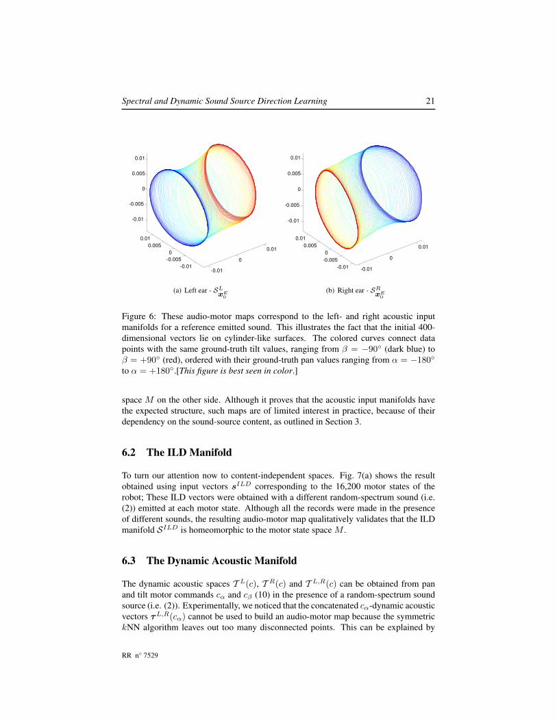
Figure 6: These audio-motor maps correspond to the left- and right acoustic inputmanifolds for a reference emitted sound. This illustrates the fact that the initial 400-dimensional vectors lie on cylinder-like surfaces. The colored curves connect datapoints with the same ground-truth tilt values, ranging from β = −90◦ (dark blue) toβ = +90◦ (red), ordered with their ground-truth pan values ranging from α = −180◦

to α = +180◦.[This figure is best seen in color.]

space M on the other side. Although it proves that the acoustic input manifolds havethe expected structure, such maps are of limited interest in practice, because of theirdependency on the sound-source content, as outlined in Section 3.

6.2 The ILD Manifold

To turn our attention now to content-independent spaces. Fig. 7(a) shows the resultobtained using input vectors sILD corresponding to the 16,200 motor states of therobot; These ILD vectors were obtained with a different random-spectrum sound (i.e.(2)) emitted at each motor state. Although all the records were made in the presenceof different sounds, the resulting audio-motor map qualitatively validates that the ILDmanifold SILD is homeomorphic to the motor state space M .

6.3 The Dynamic Acoustic Manifold

The dynamic acoustic spaces T L(c), T R(c) and T L,R(c) can be obtained from panand tilt motor commands cα and cβ (10) in the presence of a random-spectrum soundsource (i.e. (2)). Experimentally, we noticed that the concatenated cα-dynamic acousticvectors τL,R(cα) cannot be used to build an audio-motor map because the symmetrickNN algorithm leaves out too many disconnected points. This can be explained by

RR n° 7529


-0.01

0

0.01

-0.01

0

0.01

-0.015

-0.01

-0.005

0

0.005

0.01

0.015

(a) ILD manifold SILD

-0.01 -0.005 0 0.005 0.01

-0.01

-0.005

0

0.005

0.01

-0.015

-0.01

-0.005

0

0.005

0.01

0.015

(b) Concatenated dynamic acoustic manifoldT L,R(cβ)

Figure 7: Binaural manifolds built using either the ILD vectors (a) or the concatenatedcβ-dynamic acoustic vectors (b). The colored curves connect data points with the sameground-truth tilt values, ranging from β = −90◦ (dark blue) to β = +90◦ (red), or-dered with their ground-truth pan values ranging from α = −180◦ to α = +180◦.[Thisfigure is best seen in color.]

the fact that the mechanical set up used implies that pan movements induce differentsound source displacements in the robot frame depending on the current tilt position,as mentioned earlier in Section 2. One should notice, however, that tilt positions arenot conditioned by pan positions and hence one can compute an audio-motor mapfrom concatenated cβ-dynamic acoustic vectors τL,R(cβ). Fig. 7(b) shows that themanifold thus obtained, although distorted, qualitatively verifies the three criteria for ahomeomorphic mapping. Therefore, the cβ-dynamic acoustic manifold T L,R(cβ) canbe thought of as being homeomorphic to the motor state space M .

One may argue that the concatenated dynamic acoustic manifolds may be of lit-tle interest since the ILD manifold provides similar results, and this without the needof any head motion. Nevertheless, dynamic data remains extremely interesting be-cause it can by used in conjunction with a single microphone thus yielding monauralmanifolds, one for each microphone. Fig. 8(a)-(b) show audio-motor maps obtainedfrom monaural cβ−dynamic acoustic vectors τL(cβ) and τR(cβ). These plots re-veal important distortions of the manifolds due to some confusions between recordsassociated with high and low tilt positions. To overcome this problem, we removedfrom the training data set those input vectors corresponding to high and low tilt values.Fig. 8(c)-(d) shows the manifolds obtained from a subset of 10,800 motor states in therange α ∈ [−180◦, 180◦] and β ∈ [−60◦, 60◦]. These results qualitatively validate theexistence of a homeomorphism between a subset of T L(cβ) and T R(cβ) on one sideand a subset of the motor state space M on the other side.

INRIA


-0.01

0

0.01

-0.01

0

0.01

-0.01

-0.005

0

0.005

0.01

(a) Left-ear dynamic acoustic manifold T L(cβ)

-0.01

0

0.01

0.02

-0.01

0

0.01

-0.02

-0.015

-0.01

-0.005

0

0.005

0.01

0.015

(b) Right-ear dynamic acoustic manifold T R(cβ)

-0.01

0

0.01

-0.01

0

0.01

-0.015

-0.01

-0.005

0

0.005

0.01

0.015

(c) Truncated left manifold

-0.01

0

0.01

-0.01

0

0.01

-0.015

-0.01

-0.005

0

0.005

0.01

0.015

(d) Truncated right manifold

Figure 8: Monaural dynamic manifolds obtained with the whole data set (a), (b) andwith a truncated data set (c), (d). First row: all the 16,200 motor states are used.Second row: a subset of 10,800 motor states corresponding to α ∈ [−180◦, 180◦] andβ ∈ [−60◦, 60◦] is used. The color conventions are the same as above. [This figure isbest seen in color.]

6.4 Sound Localization and Missing Frequencies

All these results show that both binaural static cues (i.e. ILD vectors) and monauraldynamic cues (i.e. cβ-dynamic acoustic vectors) may be used to retrieve the directionof a sound source independently of its content. Indeed, they experimentally prove theexistence of homeomorphisms between our content-independent acoustic manifoldsand the motor-state manifold M . Therefore, the problem of localizing an unknown

RR n° 7529


sound source from a few auditory observations is equivalent to classifying a samplefrom a test-set based on training using another data set. In that sense, a major contribu-tion of this paper is to view sound localization as a classification problem, whereas thevast majority of standard approaches has used close-form solutions in order to recoverspatial (3D) parameters either from ITDs, from ILDs, or from both.

In practice we implemented a nearest neighbor classifier to assess the validity ofour sound localization framework based on content-independent acoustic vectors. Onone side, the training set SILD contains ILD vectors which are estimated using all the16,200 motor states and with the speaker emitting a single reference sound, i.e., (2)with fixed parameters. On the other side, the test set SILD is composed of ILD vectorsestimated while the speaker is emitting different random-spectrum sounds drawn froma uniform distribution at each state, i.e., (2). Given an ILD vector sILDi from thetest-set, we find its nearest neighbor sILDi in the training-set and we use its associatedground-truth motor state (αi, βi) to infer the spatial direction of the sound-source usingthe direct kinematics of the robot head (1). This allows to quantitatively evaluate ourmethod by direct comparison of the ground-truth motor-state of the tested ILD vector,i.e., (αi, βi) with the motor state (αi, βi) found with the classification method justdescribed. One can therefore define the absolute angular error Ei as follow:

Ei = |αi − αi|+ |βi − βi| (17)

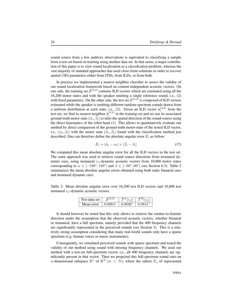
We computed this mean absolute angular error for all the ILD vectors in the test set.The same approach was used to retrieve sound source directions from monaural dy-namic cues, using monaural cβ-dynamic acoustic vectors from 10,800 motor statescorresponding to α ∈ [−180◦, 180◦] and β ∈ [−60◦, 60◦] (see Section 6.3). Table 2summarizes the mean absolute angular errors obtained using both static binaural cuesand monaural dynamic cues.

Table 2: Mean absolute angular error over 16,200 test ILD vectors and 10,800 testmonaural cβ-dynamic acoustic vectors.

Test data set SILD T L(cβ) T R(cβ)Mean error 0.0064◦ 0.0826◦ 0.0841◦

It should however be noted that this only allows to retrieve the emitter-to-listenerdirection under the assumption that the observed acoustic vectors, whether binauralor monaural, have a full spectrum, namely provided that the 400 frequency channelsare significantly represented in the perceived sounds (see Section 3). This is a rela-tively strong assumption considering that many real-world sounds only have a sparsespectrum (e.g. human voices or music instruments).

Consequently, we simulated perceived sounds with sparse spectrum and tested thevalidity of our method using sound with missing frequency channels. We used ourmethod with a test-set full-spectrum vector, i.e., all 400 frequency channels are sig-nificantly present in that vector. Then we projected this full-spectrum sound onto ann-dimensional subspace Rn of RN (n < N ), where the subset Fn of represented

INRIA


frequencies was randomly selected: Fn = {fi1 , . . . fik , . . . fin} ⊂ F (see Section 3).Finally, we compute the nearest neighbor of this sparse acoustic vector in its associatedsparse training set. In practice, in the presence of an unknown sparse-spectrum auditoryobservation, the projection could be done by applying a threshold on perceived ener-gies sLi and sRi to remove under-represented frequency channels. The mean absoluteangular error obtained with this approach was computed for the different cues, whilevarying the number of represented frequencies. We repeated this experiment with bothILD vectors and dynamic vectors.

1 50 100 150 200 250 300 350 4000

30

60

90

120

150

180

Number of frequency channels used

Mean a

bso

lute

angula

r err

or (d

egre

es)

Static ILD Vector

Tilt Dynamic Acoustic Vector (Left ear)Tilt Dynamic Acoustic Vector (Right ear)

Figure 9: Mean absolute angular error with respect to the number n of frequency chan-nels represented in the perceived sound, using ILD or cβ−dynamic acoustic vectors.

Fig. 9 summarizes the influence of the number of represented frequency channelson the mean absolute angular error. One can see that using ILD vectors, the erroris below 2◦ for sparse spectra only containing 40 frequency channels, while usingdynamic vectors one needs at least 80 channels in order to achieve the same accuracy.This result correlates with several psychophysical and behavioral studies suggestingthat the accuracy of vertical sound localization by humans is weaker for narrow-bandsound sources than for broad-band sound sources Roffler and Butler (1968), Gardnerand Gardner (1973), Butler and Helwig (1983).

7 Conclusion

Computational sound localization has long been addressed using static acoustic fea-tures such as ILD and ITD. Based on a number of psychophysical studies suggesting

RR n° 7529


that sound localization could be both a listener-dependent and a dynamic problem,we proposed a novel unsupervised learning approach making use of high-dimensionalinformation available with binaural and monaural dynamic auditory data, i.e., datagathered with a listener that moves its head while recording sounds. Our method isable to retrieve an intrinsic spatial parameterization of training sets of acoustic datain the presence of a single emitting source. This parameterization can then be asso-ciated with the ground-truth motor parameters of the listener, thus allowing to inferthe direction of unknown auditory observations. Results obtained with our approachput forward manifold learning as a powerful tool for learning sound localization withrobotic heads. They also quantitatively support several psychophysical studies imply-ing that the use of head movements in combination with the spectral richness of per-ceived sounds could improve monaural sound localization. In addition, the idea that theHRTF can be viewed as a function of motor-states, and more generally that the meaningof sensory inputs can be learned in terms of their corresponding motor actions ratherthan their corresponding external parameters (i.e. source’s position) strongly supportssensorimotor theories of human development notably put forward in Poincare (1929),Held and Hein (1963), and more recently in ORegan and Noe (2001).

In the future, we plan to test the robustness of our approach for sound localiza-tion while varying external factors, that is, by moving the emitter to various positionsaround the robot, with a large variety of emitted sounds, in different rooms with dif-ferent environmental conditions. Furthermore, we believe that a promising direction ofinvestigation towards concrete applications would consist in using the proposed modelfor the task of sound-source separation. Indeed, our technique allows to obtain low-dimensional intrinsic parameterizations of unknown acoustic observations even witha fair amount of missing frequencies. We believe that these parameterizations couldbe used to optimally cluster the spectrum of an auditory observation according to theemitters’ location, and therefore separate competing sound sources.

ReferencesAytekin, M., Moss, C. F., and Simon, J. Z. (2008). A sensorimotor approach to sound

localization. Neural Computation, 20(3), 603–635.

Belkin, M. and Niyogi, P. (2003). Laplacian eigenmaps for dimensionality reductionand data representation. Neural computation, 15(6), 1373–1396.

Blauert, J. (1997). Spatial Hearing: The Psychophysics of Human Sound Localization.MIT Press.

Butler, R. A. and Helwig, C. C. (1983). The spatial attributes of stimulus frequency inthe median sagittal plane and their role in sound localization. American Journal ofOtolaryngology, 4, 165–173.

Cherry, E. C. (1953). Some experiment on the recognition of speech, with one and withtwo ears. Journal of the Acoustical Society of America, 25(5), 975–979.

INRIA


Cox, T. and Cox, M. (1994). Multidimensional Scaling. Chapman and Hall, London.

Fisher, H. G. and Freedman, S. J. (1968). The role of the pinna in auditory localization.J. Audit. Res., 8, 15–26.

Gardner, M. B. and Gardner, R. S. (1973). Problem of localization in the medial plane:effect of pinnae cavity occlusion. Journal of the Acoustical Society of America, 53,400–408.

Greff, R. and Katz, B. F. (2007). Perceptual evaluation of HRTF notches versus peaksfor vertical localisation. In The Nineteenth International Congress on Acoustics.

Handzel, A. A. and Krishnaprasad, P. S. (2002). Biomimetic sound-source localization.IEEE Sensors Journal, 2, 607–616.

Hansard, M. and Horaud, R. P. (2010). Cyclorotation models for eyes and cameras.IEEE Transactions on System, Man, and Cybernetics–Part B: Cybernetics, 40(1),151–161.

Haykin, S. and Chen, Z. (2005). The cocktail party problem. Neural Computation, 17,1875–1902.

Hebrank, J. and Wright, D. (1974). Spectral cues used in the localisation of soundsources on the median plane. Journal of the Acoustical Society of America, 56.

Held, R. and Hein, A. (1963). Movement-produced stimulation in the development ofvisually guided behavior. J. Comp. Physiol. Psych., 56(5), 872–876.

Hornstein, J., Lopes, M., Santos-victor, J., and Lacerda, F. (2006). Sound localizationfor humanoid robots building audio-motor maps based on the hrtf. contact projectreport. In Proceedings of the IEEE/RSJ Int. Conf. on Intelligent Robots and Systems,pages 1170–1176.

King, A. J. and Schnupp, J. W. H. (2007). The auditory cortex. Current Biology, 17(7),236–239.

Kneip, L. and Baumann, C. (2008). Binaural model for artificial spatial sound localiza-tion based on interaural time delays and movements of the interaural axis. Journalof the Acoustical Society of America, 124, 3108–3119.

Lu, Y.-C. and Cooke, M. (2010). Binaural estimation of sound source distance via thedirect-to-reverberant energy ratio for static and moving sources. 18, 1793–1805.

Middlebrooks, J. C. and Green, D. M. (1991). Sound localization by human listeners.Annual Review of Psychology, 42, 135–159.

Muller, R. and Schnitzler, H.-U. (1999a). Acoustic flow perception in cf-bats: proper-ties of the available cues. Journal of the Acoustical Society of America, 105, 2959–2966.

RR n° 7529


Muller, R. and Schnitzler, H.-U. (1999b). Acoustic flow perception in cf-bats: proper-ties of the available cues. Journal of the Acoustical Society of America, 105, 2959–2966.

Muller, R. and Schnitzler, H.-U. (2001). Computational assessment of an acoustic flowhypothesis for cf-bats. In Computational models of auditory function. IOS Press.

Otani, M., Hirahara, T., and Ise, S. (2009). Numerical study on source-distance de-pendency of head-related transfer functions. Journal of the Acoustical Society ofAmerica, 125(5), 3253–61.

ORegan, K. J. and Noe, A. (2001). A sensorimotor account of vision and visual con-sciousness. Behavioral and Brain Sciences, 24, 939–1031.

Poincare, H. (1929). The Foundations of science; Science and Hypothesis, the Value ofScience, Science and Method. New York: Science Press. Translated from French byHalsted. Original title: La Valeur de la Science, 1905.

Pollack, I. and Rose, M. (1967). Effect of head movement on the localization of soundsin the equatorial plane. Percept. Psychophys., 2, 591–596.

Raspaud, M., Viste, H., and Evangelista, G. (2010). Binaural source localization byjoint estimation of ild and itd. 18(1), 68–77.

Roffler, S. K. and Butler, R. A. (1968). Factors that influence the localization of soundin the vertical plane. Journal of the Acoustical Society of America, 43, 1288–1259.

Roman, N. and Wang, D. (2008). Binaural tracking of multiple moving sources. 16(4),728–739.

Saul, L. and Roweis, S. (2003). Think globally, fit locally: unsupervised learning oflow dimensional manifolds. Journal of Machine Learning Research, 4, 119–155.

Scholkopf, B., Smola, A. J., and Muller, K. R. (1998). Nonlinear component analysisas a kernel eigenvalue problem. Neural Computation, 10, 1299–1319.

Tenenbaum, J. B., de Silva, V., and Langford, J. C. (2000). A global geometric frame-work for nonlinear dimensionality reduction. Science, 290, 2319–2323.

Thurlow, W. R. and Runge, P. S. (1967). Effect of induced head movements on lo-calization of direction of sounds. Journal of the Acoustical Society of America, 42,480–488.

Walker, V. A., Peremans, H., and Hallam, J. C. T. (1998). One tone, two ears, threedimensions: A robotic investigation of pinnae movements used by rhinolophid andhipposiderid bats. Journal of the Acoustical Society of America, 104, 569–579.

Wallach, H. (1939). On sound localization. Journal of the Acoustical Society of Amer-ica, 10, 270–274.

INRIA


Wallach, H. (1940). The role of head movements and vestibular and visual cues insound localization. J. Exp. Psychol, 27, 338–368.

Wang, D. and Brown, G. J. (2006). Computational Auditory Scene Analysis: Princi-ples, Algorithms and Applications. IEEE Press.

Wenzel, E. M. (1995). The relative contribution of interaural time and magnitude cuesto dynamic sound localization. In IEEE ASSP Workshop on Applications of SignalProcessing to Audio and Acoustics.

Willert, V., Eggert, J., Adamy, J., Stahl, R., and Koerner, E. (2006). A probabilisticmodel for binaural sound localization. 36(5), 982–994.

Woodworth, R. S. and Schlosberg, H. (1965). Experimental Psychology. Holt.

Zhang, Z. and Zha, H. (2004). Principal manifolds and nonlinear dimensionality re-duction via tangent space alignment. SIAM Journal on Scientific Computing, 26(1).

RR n° 7529

Centre de recherche INRIA Grenoble – Rhône-Alpes655, avenue de l’Europe - 38334 Montbonnot Saint-Ismier (France)

Centre de recherche INRIA Bordeaux – Sud Ouest : Domaine Universitaire - 351, cours de la Libération - 33405 Talence CedexCentre de recherche INRIA Lille – Nord Europe : Parc Scientifique de la Haute Borne - 40, avenue Halley - 59650 Villeneuve d’Ascq

Centre de recherche INRIA Nancy – Grand Est : LORIA, Technopôle de Nancy-Brabois - Campus scientifique615, rue du Jardin Botanique - BP 101 - 54602 Villers-lès-Nancy Cedex

Centre de recherche INRIA Paris – Rocquencourt : Domaine de Voluceau - Rocquencourt - BP 105 - 78153 Le Chesnay CedexCentre de recherche INRIA Rennes – Bretagne Atlantique : IRISA, Campus universitaire de Beaulieu - 35042 Rennes Cedex

Centre de recherche INRIA Saclay – Île-de-France : Parc Orsay Université - ZAC des Vignes : 4, rue Jacques Monod - 91893 Orsay CedexCentre de recherche INRIA Sophia Antipolis – Méditerranée : 2004, route des Lucioles - BP 93 - 06902 Sophia Antipolis Cedex

ÉditeurINRIA - Domaine de Voluceau - Rocquencourt, BP 105 - 78153 Le Chesnay Cedex (France)

http://www.inria.frISSN 0249-6399

Documents

Antoine Deleforge and Radu Horaud