High dimensional regression with Gaussian …...High dimensional regression with Gaussian mixtures and partially latent response variables Antoine Deleforge, Florence Forbes, and Radu

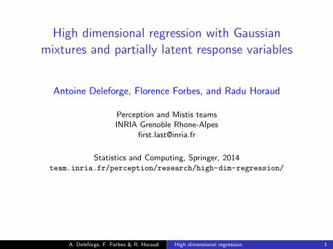
High dimensional regression with Gaussianmixtures and partially latent response variables

Antoine Deleforge, Florence Forbes, and Radu Horaud

Perception and Mistis teamsINRIA Grenoble Rhone-Alpes

[email protected]

Statistics and Computing, Springer, 2014team.inria.fr/perception/research/high-dim-regression/

A. Deleforge, F. Forbes & R. Horaud High dimensional regression 1

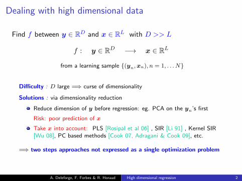
team.inria.fr/perception/research/high-dim-regression/

Dealing with high dimensional data

Find f between y ∈ RD and x ∈ RL with D >> L

f : y ∈ RD −→ x ∈ RL

from a learning sample {(yn,xn), n = 1, . . . N}

Difficulty : D large =⇒ curse of dimensionality

Solutions : via dimensionality reduction

Reduce dimension of y before regression: eg. PCA on the yn’s first

Risk: poor prediction of x

Take x into account: PLS [Rosipal et al 06] , SIR [Li 91] , Kernel SIR[Wu 08], PC based methods [Cook 07, Adragani & Cook 09], etc.

=⇒ two steps approaches not expressed as a single optimization problem


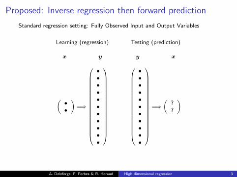
Proposed: Inverse regression then forward prediction

Standard regression setting: Fully Observed Input and Output Variables

Learning (regression) Testing (prediction)

x y y x

(••

)=⇒

•••••••••••

•••••••••••

=⇒

(??

)


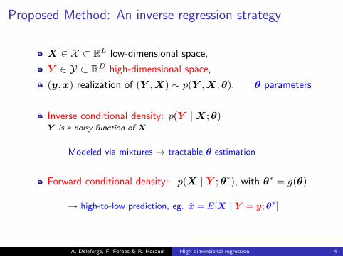
Proposed Method: An inverse regression strategy

X ∈ X ⊂ RL low-dimensional space,

Y ∈ Y ⊂ RD high-dimensional space,

(y,x) realization of (Y ,X) ∼ p(Y ,X;θ), θ parameters

Inverse conditional density: p(Y |X;θ)Y is a noisy function of X

Modeled via mixtures → tractable θ estimation

Forward conditional density: p(X | Y ;θ∗), with θ∗ = g(θ)

→ high-to-low prediction, eg. x = E[X | Y = y;θ∗]


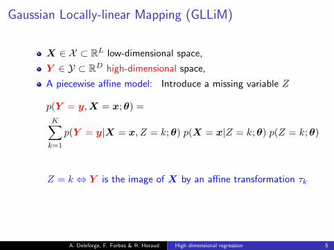
Gaussian Locally-linear Mapping (GLLiM)

X ∈ X ⊂ RL low-dimensional space,

Y ∈ Y ⊂ RD high-dimensional space,

A piecewise affine model: Introduce a missing variable Z

p(Y = y,X = x;θ) =

K∑k=1

p(Y = y|X = x, Z = k;θ) p(X = x|Z = k;θ) p(Z = k;θ)

Z = k ⇔ Y is the image of X by an affine transformation τk


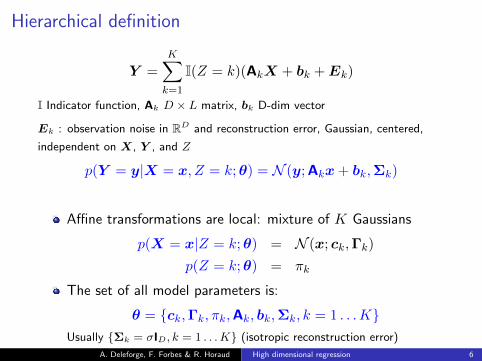
Hierarchical definition

Y =

K∑k=1

I(Z = k)(AkX + bk +Ek)

I Indicator function, Ak D × L matrix, bk D-dim vector

Ek : observation noise in RD and reconstruction error, Gaussian, centered,

independent on X, Y , and Z

p(Y = y|X = x, Z = k;θ) = N (y;Akx+ bk,Σk)

Affine transformations are local: mixture of K Gaussians

p(X = x|Z = k;θ) = N (x; ck,Γk)

p(Z = k;θ) = πk

The set of all model parameters is:

θ = {ck,Γk, πk,Ak, bk,Σk, k = 1 . . .K}Usually {Σk = σID, k = 1 . . .K} (isotropic reconstruction error)


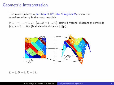
Geometric Interpretation

This model induces a partition of RL into K regions Rk where thetransformation τk is the most probable.

If |Γ1| = · · · = |ΓK |: {Rk, k = 1 . . .K} define a Voronoi diagram of centroids{ck, k = 1 . . .K} (Mahalanobis distance ||.||Γ).

L = 2, D = 3,K = 15.


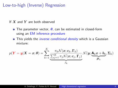
Low-to-high (Inverse) Regression

If X and Y are both observed

The parameter vector, θ, can be estimated in closed-formusing an EM inference procedure

This yields the inverse conditional density which is a Gaussianmixture:

p(Y = y|X = x;θ) =

K∑k=1

πkN (x; ck,Γk)∑Kj=1 πjN (x; cj ,Γj)︸︷︷︸

βk

N (y;Akx+ bk︸︷︷︸µk

,Σk)


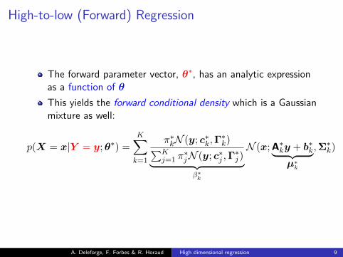
High-to-low (Forward) Regression

The forward parameter vector, θ∗, has an analytic expressionas a function of θ

This yields the forward conditional density which is a Gaussianmixture as well:

p(X = x|Y = y;θ∗) =

K∑k=1

π∗kN (y; c∗k,Γ∗k)∑K

j=1 π∗jN (y; c∗j ,Γ

∗j )︸︷︷︸

β∗k

N (x;A∗ky + b∗k︸︷︷︸µ∗k

,Σ∗k)


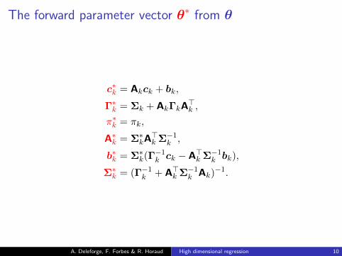
The forward parameter vector θ∗ from θ

c∗k = Akck + bk,

Γ∗k = Σk + AkΓkA>k ,

π∗k = πk,

A∗k = Σ∗kA>k Σ−1k ,

b∗k = Σ∗k(Γ−1k ck − A>k Σ−1k bk),

Σ∗k = (Γ−1k + A>k Σ−1k Ak)−1.


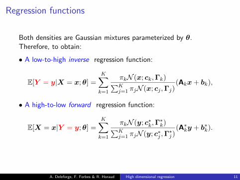
Regression functions

Both densities are Gaussian mixtures parameterized by θ.Therefore, to obtain:

• A low-to-high inverse regression function:

E[Y = y|X = x;θ] =

K∑k=1

πkN (x; ck,Γk)∑Kj=1 πjN (x; cj ,Γj)

(Akx+ bk),

• A high-to-low forward regression function:

E[X = x|Y = y;θ] =

K∑k=1

πkN (y; c∗k,Γ∗k)∑K

j=1 πjN (y; c∗j ,Γ∗j )(A∗ky + b∗k).


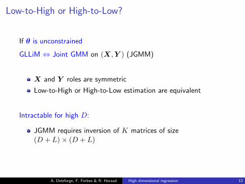
Low-to-High or High-to-Low?

If θ is unconstrained

GLLiM ⇔ Joint GMM on (X,Y ) (JGMM)

X and Y roles are symmetric

Low-to-High or High-to-Low estimation are equivalent

Intractable for high D:

JGMM requires inversion of K matrices of size(D + L)× (D + L)


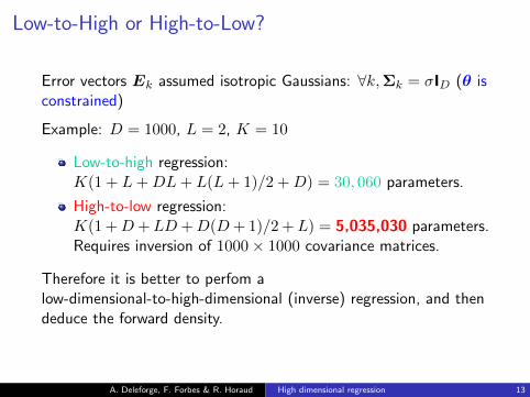
Low-to-High or High-to-Low?

Error vectors Ek assumed isotropic Gaussians: ∀k,Σk = σID (θ isconstrained)

Example: D = 1000, L = 2, K = 10

Low-to-high regression:K(1 + L+DL+ L(L+ 1)/2 +D) = 30, 060 parameters.

High-to-low regression:K(1 +D+LD+D(D+ 1)/2 +L) = 5,035,030 parameters.Requires inversion of 1000× 1000 covariance matrices.

Therefore it is better to perfom alow-dimensional-to-high-dimensional (inverse) regression, and thendeduce the forward density.


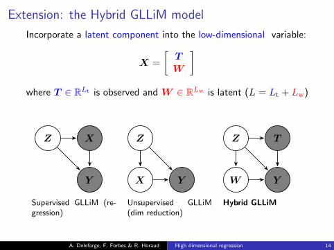
Extension: the Hybrid GLLiM model

Incorporate a latent component into the low-dimensional variable:

X =

[TW

]where T ∈ RLt is observed and W ∈ RLw is latent (L = Lt + Lw)

Z X

Y

Z

X Y

Z

W

T

Y

Supervised GLLiM (re-gression)

Unsupervised GLLiM(dim reduction)

Hybrid GLLiM


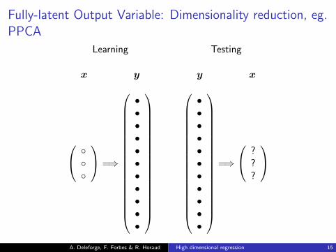
Fully-latent Output Variable: Dimensionality reduction, eg.PPCA

Learning Testing

x y y x

◦◦◦

=⇒

•••••••••••

•••••••••••

=⇒

???


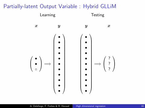
Partially-latent Output Variable : Hybrid GLLiM

Learning Testing

x y y x

••◦

=⇒

•••••••••••

•••••••••••

=⇒

???


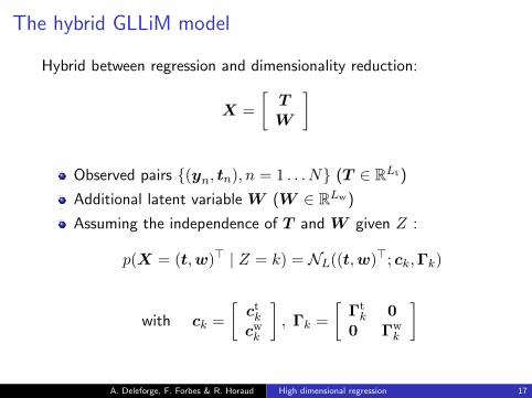
The hybrid GLLiM model

Hybrid between regression and dimensionality reduction:

X =

[TW

]

Observed pairs {(yn, tn), n = 1 . . . N} (T ∈ RLt)

Additional latent variable W (W ∈ RLw)

Assuming the independence of T and W given Z :

p(X = (t,w)> | Z = k) = NL((t,w)>; ck,Γk)

with ck =

[ctkcwk

], Γk =

[Γtk 0

0 Γwk

]


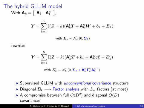
The hybrid GLLiM modelWith Ak =

[Atk Aw

k

],

Y =

K∑k=1

I(Z = k)(AtkT + Aw

kW + bk +Ek)

with Ek ∼ ND(0,Σk)

rewrites

Y =

K∑k=1

I(Z = k)(AtkT + bk + Aw

k cwk +E′k)

with E′k ∼ ND(0,Σk + Awk Γw

k Aw>k )

Supervised GLLiM with unconventional covariance structure

Diagonal Σk −→ Factor analysis with Lw factors (at most)

A compromise between full O(D2) and diagonal O(D)covariances


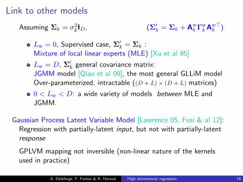
Link to other models

Assuming Σk = σ2kID, (Σ′k = Σk + AwkΓw

k Aw>k )

Lw = 0, Supervised case, Σ′k = Σk :Mixture of local linear experts (MLE) [Xu et al 95]

Lw = D, Σ′k general covariance matrix:JGMM model [Qiao et al 09], the most general GLLiM modelOver-parameterized, intractable ((D + L)× (D + L) matrices)

0 < Lw < D: a wide variety of models between MLE andJGMM.

Gaussian Process Latent Variable Model [Lawrence 05, Fusi & al 12]:Regression with partially-latent input, but not with partially-latentresponse

GPLVM mapping not inversible (non-linear nature of the kernelsused in practice)


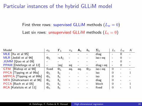
Particular instances of the hybrid GLLiM model

First three rows: supervised GLLiM methods (Lw = 0)

Last six rows: unsupervised GLLiM methods (Lt = 0)

Model ck Γk πk Ak bk Σk Lt Lw KMLE [Xu et al 95] - - - - - diag - 0 -MLR [Jedidi et al 96] 0L ∞IL - - - iso+eq - 0 -JGMM [Qiao et al 09] - - - - - - - 0 -PPAM [Deleforge et al 12] - |eq| eq - - diag+eq - 0 -GTM [Bishop et al 98] fixed 0L eq. eq. 0D iso+eq 0 - -PPCA [Tipping et al 99a] 0L IL - - - iso 0 - 1MPPCA [Tipping et al 99b] 0L IL - - - iso 0 - -MFA [Ghahramani et al 96] 0L IL - - - diag 0 - -PCCA [Bach et al 05] 0L IL - - - block 0 - 1RCA [Kalaitzis et al 11] 0L IL - - - fixed 0 - 1


Expectation Maximization for Hybrid GLLiM

2 data augmentation schemes: Convergence speed/M-step tractability tradeoff

(other: Alternating ECM [Meng & Rubin 97] eg. for MFA [McLachlan et al 03])

General hybrid GLLiM-EM: augmenting with both (Z,W )

Closed-form expressions for a wide range of{Γk,Σk, k = 1 . . .K}

Marginal-hGLLiM: integrating out the W

Less general, closed form only for distinc isotropic{Σk, k = 1 . . .K}Algorithmic insight: alternation of a regression & reductionstepNatural initialization strategy


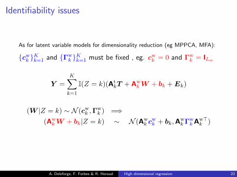
Identifiability issues

As for latent variable models for dimensionality reduction (eg MPPCA, MFA):

{cwk }Kk=1 and {Γwk }Kk=1 must be fixed , eg. cwk = 0 and Γw

k = ILw

Y =

K∑k=1

I(Z = k)(AtkT + Aw

kW + bk +Ek)

(W |Z = k) ∼ N (cwk ,Γwk ) =⇒

(AwkW + bk|Z = k) ∼ N (Aw

k cwk + bk,A

wkΓw

k Aw>k )


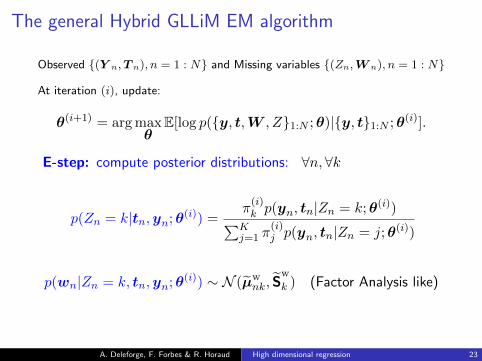
The general Hybrid GLLiM EM algorithm

Observed {(Y n,T n), n = 1 : N} and Missing variables {(Zn,W n), n = 1 : N}

At iteration (i), update:

θ(i+1) = argmaxθ

E[log p({y, t,W , Z}1:N ;θ)|{y, t}1:N ;θ(i)].

E-step: compute posterior distributions: ∀n, ∀k

p(Zn = k|tn,yn;θ(i)) =π(i)k p(yn, tn|Zn = k;θ(i))∑K

j=1 π(i)j p(yn, tn|Zn = j;θ(i))

p(wn|Zn = k, tn,yn;θ(i)) ∼ N (µw

nk, Sw

k ) (Factor Analysis like)


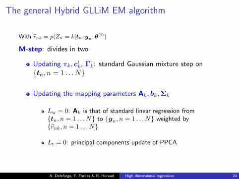
The general Hybrid GLLiM EM algorithm

With rnk = p(Zn = k|tn,yn;θ(i))

M-step: divides in two

Updating πk, ctk, Γt

k: standard Gaussian mixture step on{tn, n = 1 . . . N}

Updating the mapping parameters Ak, bk,Σk

Lw = 0: Ak is that of standard linear regression from{tn, n = 1 . . . N} to {yn, n = 1 . . . N} weighted by{rnk, n = 1 . . . N}

Lt = 0: principal components update of PPCA


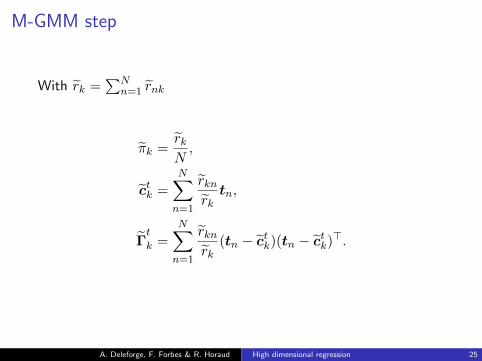
M-GMM step

With rk =∑N

n=1 rnk

πk =rkN,

ctk =

N∑n=1

rknrktn,

Γt

k =

N∑n=1

rknrk

(tn − ctk)(tn − ctk)>.


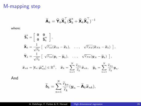
M-mapping step

Ak = YkX>k (S

x

k + XkX>k )−1

where:

Sx

k =

[0 0

0 Sw

k

],

Xk =1√rk

[ √r1k(x1k − xk), . . . ,

√rNk(xNk − xk)

],

Yk =1√rk

[ √r1k(y1 − yk), . . . ,

√rNk(yN − yk)

],

xnk = [tn; µwnk] ∈ RL, xk =

N∑n=1

rknrkxnk, yk =

N∑n=1

rknrkyn.

And

bk =

N∑n=1

rknrk

(yn − Akxnk),


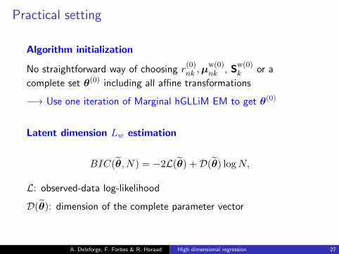
Practical setting

Algorithm initialization

No straightforward way of choosing r(0)nk ,µ

w(0)nk , S

w(0)k or a

complete set θ(0) including all affine transformations

−→ Use one iteration of Marginal hGLLiM EM to get θ(0)

Latent dimension Lw estimation

BIC(θ, N) = −2L(θ) +D(θ) logN,

L: observed-data log-likelihood

D(θ): dimension of the complete parameter vector


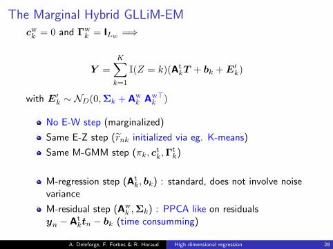
The Marginal Hybrid GLLiM-EM

cwk = 0 and Γwk = ILw =⇒

Y =

K∑k=1

I(Z = k)(AtkT + bk +E

′k)

with E′k ∼ ND(0,Σk + Awk Aw>

k )

No E-W step (marginalized)

Same E-Z step (rnk initialized via eg. K-means)

Same M-GMM step (πk, ctk,Γ

tk)

M-regression step (Atk, bk) : standard, does not involve noise

variance

M-residual step (Awk ,Σk) : PPCA like on residuals

yn − Atktn − bk (time consumming)


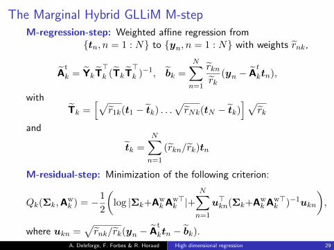
The Marginal Hybrid GLLiM M-stepM-regression-step: Weighted affine regression from

{tn, n = 1 : N} to {yn, n = 1 : N} with weights rnk,

At

k = YkT>k (TkT

>k )−1, bk =

N∑n=1

rknrk

(yn − At

ktn),

withTk =

[√r1k(t1 − tk) . . .

√rNk(tN − tk)

]√rk

and

tk =

N∑n=1

(rkn/rk)tn

M-residual-step: Minimization of the following criterion:

Qk(Σk,Awk ) = −

1

2

(log |Σk+Aw

k Aw>k |+

N∑n=1

u>kn(Σk+Awk Aw>

k )−1ukn

),

where ukn =√rnk/rk(yn − A

t

ktn − bk).A. Deleforge, F. Forbes & R. Horaud High dimensional regression 29

Experiments and results


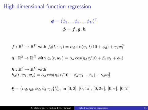
High dimensional function regression

φ = (φ1 . . . φd . . . φD)>

φ = f , g,h

f : R2 → RD with fd(t, w1) = αd cos(ηd t/10 + φd) + γdw31

g : R2 → RD with gd(t, w1) = αd cos(ηd t/10 + βdw1 + φd)

h : R3 → RD withhd(t, w1, w2) = αd cos(ηd t/10 + βdw1 + φd) + γdw

32

ξ = {αd, ηd, φd, βd, γd}Dd=1 in [0, 2], [0, 4π], [0, 2π], [0, π], [0, 2]


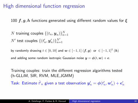
High dimensional function regression

100 f , g,h functions generated using different random values for ξ

N training couples {(tn,yn)}Nn=1

N ′ test couples {(t′n,y′n)}N′

n=1

by randomly drawing t ∈ [0, 10] and w ∈ [−1, 1] (f , g) or ∈ [−1, 1]2 (h)

and adding some random isotropic Gaussian noise y = φ(t,w) + e.

Training couples: train the different regression algorithms tested(h-GLLiM, SIR, RVM, MLE,JGMM)

Task: Estimate t′n given a test observation y′n = φ(t′n,w′n) + e

′n


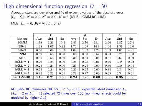
High dimensional function regression D = 50Average, standard deviation and % of extreme values of the absolute error|t′n − t′n|. N = 200, N ′ = 200, K = 5 (MLE, JGMM,hGLLiM)

MLE: Lw = 0, JGMM : Lw > D

f g hMethod Avg Std Ex Avg Std Ex Avg Std ExJGMM 1.78 2.21 19.5 2.45 2.76 28.4 2.26 2.87 22.4SIR-1 1.28 1.07 5.92 1.73 1.39 14.9 1.64 1.31 13.0SIR-2 0.60 0.69 1.02 1.02 1.02 4.20 1.03 1.06 4.91RVM 0.59 0.53 0.30 0.86 0.68 0.52 0.93 0.75 1.00MLE 0.36 0.53 0.50 0.36 0.34 0.04 0.61 0.69 0.99

hGLLiM-1 0.20 0.24 0.00 0.25 0.28 0.01 0.46 0.48 0.22hGLLiM-2 0.23 0.24 0.00 0.25 0.25 0.00 0.36 0.38 0.04hGLLiM-3 0.24 0.24 0.00 0.26 0.25 0.00 0.34 0.34 0.01hGLLiM-4 0.23 0.23 0.01 0.28 0.27 0.00 0.35 0.34 0.01

hGLLiM-BIC 0.18 0.21 0.00 0.24 0.26 0.00 0.33 0.35 0.06

hGLLiM-BIC minimizes BIC for 0 < Lw < 10: expected latent dimension Lw

(Lw = 2 or Lw = 1) selected 72 times over 100 (non-linear effects could bemodeled by higher Lw)


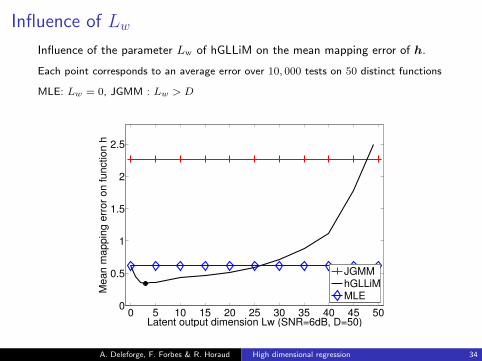
Influence of LwInfluence of the parameter Lw of hGLLiM on the mean mapping error of h.

Each point corresponds to an average error over 10, 000 tests on 50 distinct functions

MLE: Lw = 0, JGMM : Lw > D

0 5 10 15 20 25 30 35 40 45 500

0.5

1

1.5

2

2.5

Latent output dimension Lw (SNR=6dB, D=50)

Meanmappingerroronfunctionh

JGMMhGLLiMMLE


Influence of K

Influence of K in MLE, JGMM and hGLLiM-3 on the mean mapping error ofsynthetic function h.


2 4 6 8 10 12 14 16 18 200

0.5

1

1.5

2

Number of mixture components K (SNR=6dB, D=50)

Meanmappingerroronfunctionh JGMM

SIR−1SIR−2RVMMLEhGLLiM−3

Errors generally decrease with K. Overfitting for K > 10 for JGMM


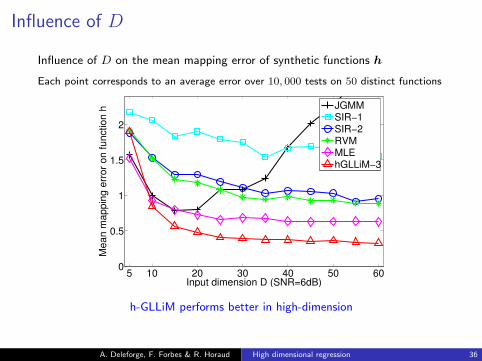
Influence of D

Influence of D on the mean mapping error of synthetic functions h


5 10 20 30 40 50 600

0.5

1

1.5

2

Input dimension D (SNR=6dB)

Me

an

ma

pp

ing

err

or

on

fun

ctio

nh JGMM


h-GLLiM performs better in high-dimension


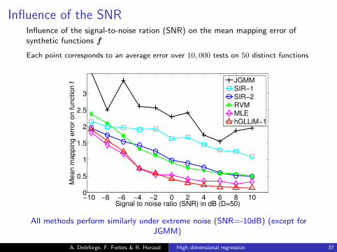
Influence of the SNRInfluence of the signal-to-noise ration (SNR) on the mean mapping error ofsynthetic functions f


−10 −8 −6 −4 −2 0 2 4 6 8 100

0.5

1

1.5

2

2.5

3

Signal to noise ratio (SNR) in dB (D=50)

Meanmappingerroronfunctionf JGMM


All methods perform similarly under extreme noise (SNR=-10dB) (except forJGMM)


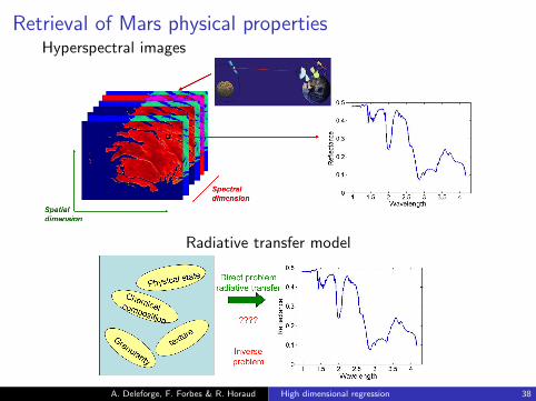
Retrieval of Mars physical propertiesHyperspectral images

Radiative transfer model


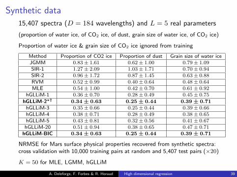
Synthetic data

15,407 spectra (D = 184 wavelengths) and L = 5 real parameters

(proportion of water ice, of CO2 ice, of dust, grain size of water ice, of CO2 ice)

Proportion of water ice & grain size of CO2 ice ignored from training

Method Proportion of CO2 ice Proportion of dust Grain size of water iceJGMM 0.83± 1.61 0.62± 1.00 0.79± 1.09SIR-1 1.27± 2.09 1.03± 1.71 0.70± 0.94SIR-2 0.96± 1.72 0.87± 1.45 0.63± 0.88RVM 0.52± 0.99 0.40± 0.64 0.48± 0.64MLE 0.54± 1.00 0.42± 0.70 0.61± 0.92

hGLLiM-1 0.36± 0.70 0.28± 0.49 0.45± 0.75

hGLLiM-2∗† 0.34 ± 0.63 0.25 ± 0.44 0.39 ± 0.71hGLLiM-3 0.35± 0.66 0.25± 0.44 0.39± 0.66hGLLiM-4 0.38± 0.71 0.28± 0.49 0.38± 0.65hGLLiM-5 0.43± 0.81 0.32± 0.56 0.41± 0.67

hGLLiM-20 0.51± 0.94 0.38± 0.65 0.47± 0.71hGLLiM-BIC 0.34 ± 0.63 0.25 ± 0.44 0.39 ± 0.71

NRMSE for Mars surface physical properties recovered from synthetic spectra:cross validation with 10,000 training pairs at random and 5,407 test pairs (×20)

K = 50 for MLE, LGMM, hGLLiM


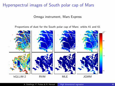
Hyperspectral images of South polar cap of Mars

Omega instrument, Mars Express

Proportions of dust for the South polar cap of Mars: orbits 41 and 61

hGLLiM-2 RVM MLE JGMM


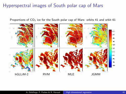
Hyperspectral images of South polar cap of Mars

Proportions of CO2 ice for the South polar cap of Mars: orbits 41 and orbit 61

hGLLiM-2 RVM MLE JGMM


Conclusion/ Perspectives

We propose a novel inverse approach to high-dimensionalregression based on mixture- and latent-variable models.

Latent component allows to capture behaviors that cannot beeasily modeled

Adaptive latent dimension Lw selection

More complex dependencies between variables (eg.(Z1 . . . ZN ) is a MRF)

More complex noise models, eg, Student for outliersaccommodation and robustness

Matlab code available at: https://team.inria.fr/perception/gllim_toolbox/

A. Deleforge, F. Forbes and R. Horaud, High-Dimensional Regression with Gaussian Mixtures and Partially-LatentResponse Variables. Statistics & Computing.

A. Deleforge, F. Forbes and R. Horaud, Hyper-spectral Image Analysis with Partially-Latent Regression. EUSIPCO,Lisbon, Portugal, September 2014.


https://team.inria.fr/perception/gllim_toolbox/

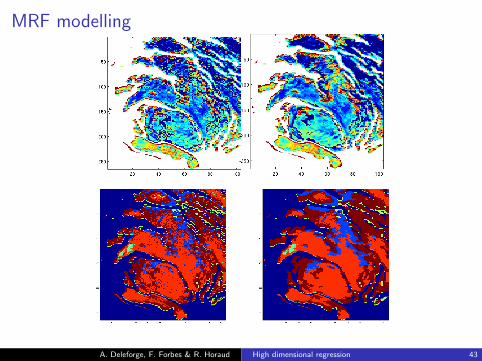
MRF modelling


Documents

High dimensional regression with Gaussian …...High dimensional regression with Gaussian mixtures and partially latent response variables Antoine Deleforge, Florence Forbes, and Radu