Embed Size (px)
Citation preview
HAL Id: halshs-00359850https://halshs.archives-ouvertes.fr/halshs-00359850
Submitted on 31 Mar 2009
HAL is a multi-disciplinary open accessarchive for the deposit and dissemination of sci-entific research documents, whether they are pub-lished or not. The documents may come fromteaching and research institutions in France orabroad, or from public or private research centers.
L’archive ouverte pluridisciplinaire HAL, estdestinée au dépôt et à la diffusion de documentsscientifiques de niveau recherche, publiés ou non,émanant des établissements d’enseignement et derecherche français ou étrangers, des laboratoirespublics ou privés.
Antidumping Procedures and Macroeconomic Factors:A Comparison between the United States and the
European UnionMustapha Sadni Jallab, Monnet Gbakou, René Sandretto
To cite this version:Mustapha Sadni Jallab, Monnet Gbakou, René Sandretto. Antidumping Procedures and Macroeco-nomic Factors: A Comparison between the United States and the European Union. Global EconomyJournal, The Berkeley Electronic Press, 2008, 3 (article 5), s.p. <halshs-00359850>
Antidumping Procedures and Macroeconomic Factors: An Estimation for
the United States and the European Union 1
Mustapha Sadni-Jallab*a
Patrick Monnet Gbakou **b
René Sandretto*c
*Université Lyon 2, GATE
** Ecole Normale Supérieure, GATE
Abstract:
This paper examines the relationship between antidumping filings and macroeconomic factors
in the US and the EU. A highly dispersed distribution of the number of openings of
antidumping proceduresis confirmed with an over-dispersion test, which leads us to estimate a
negative binomial rather than a Poisson model. Results of this estimation suggest that a real
appreciation of the filing country‟s currency significantly increases the number of openings of
antidumping inquiries both in the US and the EU. Fluctuations in the level of economic
activity also influence antidumping filings in the US significantly: as one would expect, real
GDP growth is negatively related to filings. However, we could not establish such a
relationship in the EU. Lastly, increases in the import penetration rate appear to significantly
increase antidumping filings in the US. Surprisingly, this relationship turns out to be the
inverse in Europe. The particular time period selected assess the damage from dumping has a
significant impact on our findings.
****************************
JEL Classification : F13 L5- L13
Key words : Dollar Euro Exchange Rate, Antidumping initiations, Negative Binomial Model
1 We are grateful to Vincent Aussilloux (European Commission, DG Trade), Hylke Vandenbussche (Catholic
University of Leuven), Thomas Prusa (Rutger University, New Brunswick and NBER) and Robert Feinberg
(American University Washington) for their helpful comments and suggestions. Any errors are, of
course, the sole responsibility of the authors.
a Corresponding author: Phone#: +33 (0) 472 86 61 05. Fax: +33 (0) 472 86 60 90
E-mail address: [email protected]
c E-mail address: [email protected]
1. Introduction
International trade relations are increasingly influenced by conflicts caused by “unfair
competition” (actual or perceived). The resolution of these conflicts often takes the form of
managed trade agreements (such as “voluntary” export retrains or “voluntary” import
expansions). It may also lead to unilateral sanctions against unfair countries. Such measures
have ambiguous effects:
- On the one hand, it may be that these national decisions fundamentally support the
functioning of a GATT-WTO system which was not designed to resolve the new
competition problems on a multilateral basis and which is not yet able to do so.
- On the other hand, it may be that these unilateral or bilateral solutions contribute
erosion the efficiency of the GATT-WTO system, and may even pervert it, inasmuch as
they become an additional source of trade restrictions of a new kind: a protectionism
based on the diversion or even the perversion of international rules.
Typically this new protectionism consists in diverting the WTO rules from their objectives, by
using antidumping procedures2 not to promote fairness, but to protect domestic industries.
The increase in antidumping cases leads us to question whether the procedure is really
appropriate to its objective. Does it redress unfairness or does it create it? As the procedure
has been designed and as it is applied, does it not further the development of a hidden
protectionism, a protectionism which is camouflaging itself by putting on the cloak of fairness
and the enforcement of international order?
The antidumping measures instituted by the GATT (in its article 6) and specified by the
Tokyo antidumping code and its revision during the Uruguay Rounds consist of three stages:
first, the claim admissibility is examined, then the dumping margin is estimated, and last the
damages‟ reality and importance are assessed. If the investigations determine that dumping is
occurring and causing material injury, the national authorities impose an antidumping duty
(tariff) on dumped imports equal to difference between the actual and the “fair” price, so as to
offset the difference between the dumped price and the normal price. Another solution can be
a commitment of the exporter to increase the price (price undertaking), to reduce the export
quantities (such as a “voluntary” export restraint) or any other agreement which reduces the
quantity of the alleged dumped imports3.
2 Dumping literally means “to clear away or to remove”. It has come to mean “to get rid of merchandises at any
price.” 3 These decisions can be made prior to the conclusion of the investigation.
In order to be admissible, a complaint must meet three conditions:
1. Petitioners must be supported by a significant part of the import-competing industry.
2. Petitioners must provide certain information related to the alleged dumping practice,
namely the amounts by which the import price has been reduced and the import quantities
have increased.
3. The similarity of the good produced by the plaintiffs to the import good. Only those
companies which produce a good considered to be sufficiently similar to the alleged
dumped import product are entitled to lodge a complaint.
Empirical analyses of antidumping can be based on any one of three main approaches:
simulation, case study and econometric analysis. Simulation is probably the most limited
method, usually relying on static partial (sometimes general) equilibrium models which
require questionable simplifying assumptions and calibration methods to establish the price
elasticities and cross-price demand coefficients which characterize the industry (Maur, 1999).
Case studies and econometric methods seem more promising as far as antidumping is
concerned. Econometric methods in particular enable us to develop a dynamic model of
macroeconomic factors prior to, during, and following antidumping actions, thus directly
estimating the impacts of the decisions. The purpose of this paper is to analyse the influences
of some macroeconomic factors on the number of antidumping initiations in the United States
and in the European Union over the period 1990-2002. This investigation draws upon and
seeks to provide an extension to previous papers studying this issue.
In a pioneering paper, R. Feinberg (1989), investigated the causes of antidumping filings in
the United States between 1982 and 1987 with a Tobit model. He focused his explanation on
the 4 countries which are mostl often targeted by the US antidumping authorities: Japan,
Brazil, Mexico and South Korea. Feinberg established that fluctuations in the real exchange
rate are a significant factor in the opening of inquiries, especially for Japan. More precisely,
he showed that the increase in antidumping procedures between 1982 and 1987 was
significantly related to the weakness of the US dollar. In addition, Feinberg found evidence of
a negative impact of growth in GDP on the number of filings. However, the discreet nature of
the values taken by the number of openings of inquiries induces us to question the
appropriateness of Tobit method.
More recently, Feinberg (2003) used a negative binomial model in order to estimate the
determinants of quarterly antidumping US petitions between 1981 and 1998. His conclusion
was quite different: over this last period, US antidumping filings rose with the appreciation
(not the depreciation) of the US dollar. Knetter and Prusa (2003) used the same technique
(negative binomial estimation) for four of the most important antidumping users: Australia,
Canada, the European Union and the United States. In Knetter and Prusa, the dependant
variable is the number of filings occurring every year between 1980 and 1998. Surprisingly,
neither Feinberg nor Knetter and Prusa take into account the possible influence of the import
penetration rate. In our opinion, this macroeconomic variable must be considered for at least
three reasons:
- First an increase in the rate of import penetration means (or can be perceived to mean)
more rigorous foreign competition.
- Second the proof of material injury requires showing that the industry has experienced
a sharp increase in imports.
- Third the new WTO antidumping code (1994) reinforces the obligation of the
reporting country to establish a causal relationship between the dumped imports and the
damage suffered by the complainant industry.
Furthermore, former studies neglected the impact of the period used to evaluate the damage.
In Section 2, we first describe the data and the variables used in the analysis. In Section 3, we
present the model and the estimation method which seems the most appropriate based on a
preliminary test of over-dispersion. Finally, in Section 4 we present and interpret our main
results and in Section 5 we present our main conclusions.
2. Data, macroeconomic variables and relationships
Our objective is to test the following hypotheses, both in the United States and in the
European Union:
H1. The number of antidumping filings increases with the real appreciation of the
reporting country‟s currency.4
H2. The number of inquiries opened decreases with an increase in the rate of growth of
the import country‟s real GDP. The sensitivity of the business community to perceived
foreign unfair pricing behavior is increased in an economic slump, as is the incentive of
foreign firms to cut prices in order to maintain export volumes. At the same time, it
becomes easier for the importing country to prove an injury during a slump or downturn
in the economy.
4 The literature on „monetary protectionism‟ notes that a country may devalue its domestic currency in order to
boost its exports and improve its competitiveness in the trading partners‟ markets. However, such „monetary
dumping‟ is not subject to the WTO antidumping code.
H3. The number of antidumping actions rises with an increase in the rate of import
penetration5 in the filing country.
2.1. Data
Most of the data used in this paper have been drawn from the WTO Trade Policies Review
Division. Data on initiations of antidumping actions between 1990 and 2002 come from the
WTO antidumping data base. The data are available, because WTO members are under a
continuing obligation to report their antidumping actions to the WTO Secretariat (article VI).
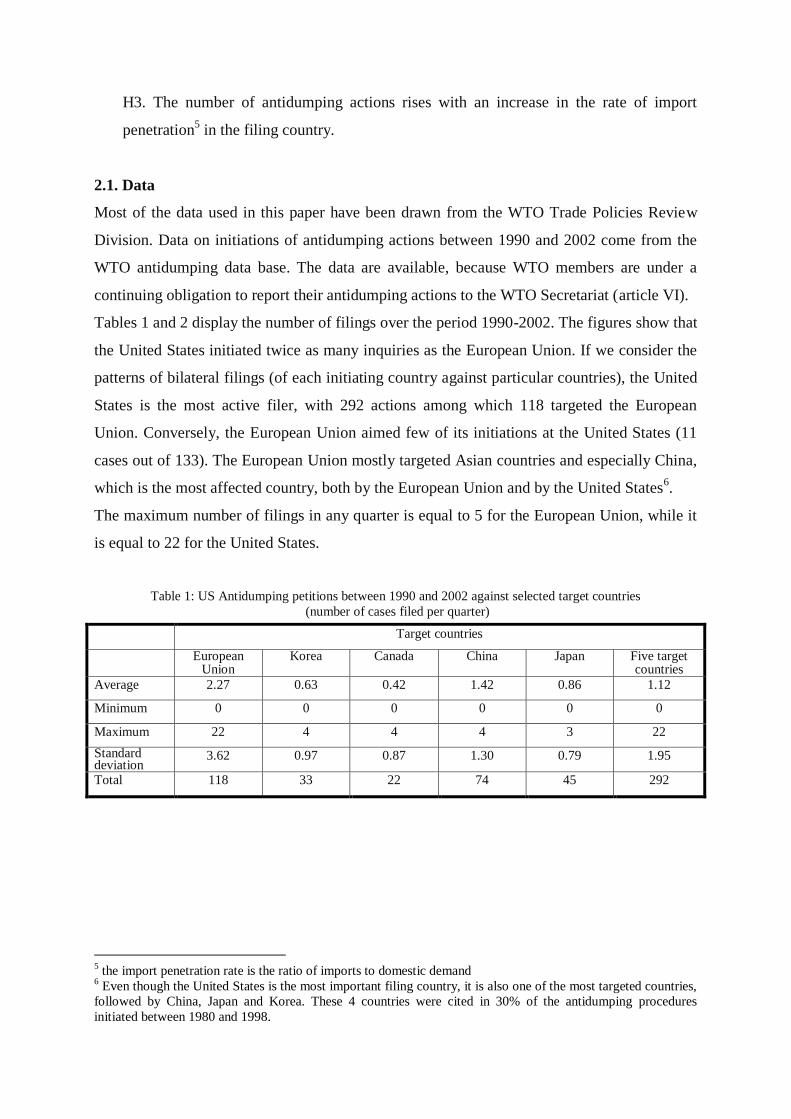
Tables 1 and 2 display the number of filings over the period 1990-2002. The figures show that
the United States initiated twice as many inquiries as the European Union. If we consider the
patterns of bilateral filings (of each initiating country against particular countries), the United
States is the most active filer, with 292 actions among which 118 targeted the European
Union. Conversely, the European Union aimed few of its initiations at the United States (11
cases out of 133). The European Union mostly targeted Asian countries and especially China,
which is the most affected country, both by the European Union and by the United States6.
The maximum number of filings in any quarter is equal to 5 for the European Union, while it
is equal to 22 for the United States.
Table 1: US Antidumping petitions between 1990 and 2002 against selected target countries
(number of cases filed per quarter)
Target countries
European Union
Korea Canada China Japan Five target countries
Average 2.27 0.63 0.42 1.42 0.86 1.12
Minimum 0 0 0 0 0 0
Maximum 22 4 4 4 3 22
Standard deviation
3.62 0.97 0.87 1.30 0.79 1.95
Total 118 33 22 74 45 292
5 the import penetration rate is the ratio of imports to domestic demand
6 Even though the United States is the most important filing country, it is also one of the most targeted countries,
followed by China, Japan and Korea. These 4 countries were cited in 30% of the antidumping procedures
initiated between 1980 and 1998.
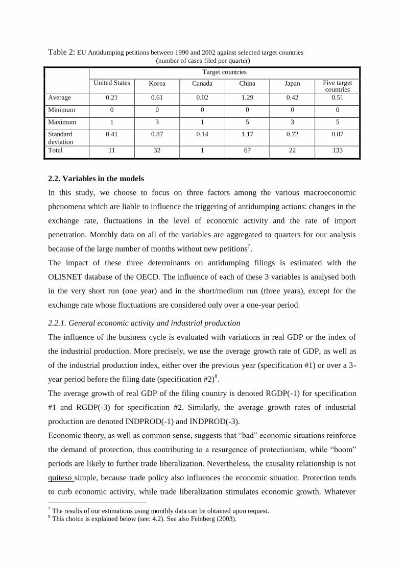
Table 2: EU Antidumping petitions between 1990 and 2002 against selected target countries
(number of cases filed per quarter)
Target countries
United States Korea Canada China Japan Five target countries
Average 0.21 0.61 0.02 1.29 0.42 0.51
Minimum 0 0 0 0 0 0
Maximum 1 3 1 5 3 5
Standard
deviation
0.41 0.87 0.14 1.17 0.72 0.87
Total 11 32 1 67 22 133
2.2. Variables in the models
In this study, we choose to focus on three factors among the various macroeconomic
phenomena which are liable to influence the triggering of antidumping actions: changes in the
exchange rate, fluctuations in the level of economic activity and the rate of import
penetration. Monthly data on all of the variables are aggregated to quarters for our analysis
because of the large number of months without new petitions7.
The impact of these three determinants on antidumping filings is estimated with the
OLISNET database of the OECD. The influence of each of these 3 variables is analysed both
in the very short run (one year) and in the short/medium run (three years), except for the
exchange rate whose fluctuations are considered only over a one-year period.
2.2.1. General economic activity and industrial production
The influence of the business cycle is evaluated with variations in real GDP or the index of
the industrial production. More precisely, we use the average growth rate of GDP, as well as
of the industrial production index, either over the previous year (specification #1) or over a 3-
year period before the filing date (specification #2)8.
The average growth of real GDP of the filing country is denoted RGDP(-1) for specification
#1 and RGDP(-3) for specification #2. Similarly, the average growth rates of industrial
production are denoted INDPROD(-1) and INDPROD(-3).
Economic theory, as well as common sense, suggests that “bad” economic situations reinforce
the demand of protection, thus contributing to a resurgence of protectionism, while “boom”
periods are likely to further trade liberalization. Nevertheless, the causality relationship is not
quiteso simple, because trade policy also influences the economic situation. Protection tends
to curb economic activity, while trade liberalization stimulates economic growth. Whatever
7 The results of our estimations using monthly data can be obtained upon request.
8 This choice is explained below (see: 4.2). See also Feinberg (2003).
the causal relationship might be, we can expect that filings are negatively related to the
business cycle. A glance at the data confirms this relationship. For example, in 1992, an
economic slump year, the number of antidumping procedures significantly increased9.
2.2.2. The force of international competition
The intensity of foreign competition suffered by country i is measured by the rate of import
penetration (denoted RIMPi):
RIMPi = i
jij
DD
M
With M ij the imports of product j by country i (respectively the US and the EU) and
j
ijM its total imports.
For the purposes of this paper, we consider the EU, like the US, as one single commercial
entity, which means that we take into account only imports from extra-EU countries10
.
DDi is the domestic demand in country i
DDi = PrCi + PuCi + INVi
With:
PrCi the private consumption in country i
PuCi the public consumption in country i
INVi the investments in country i
Logically, an increase in the rate of import penetration should lead to greater demands
forprotection in the importing country. Consequently, filings should be positively related to
the import penetration rate.
In our estimations, as for the GDP, we consider both 1-year and the 3-year average import
penetration rates prior to the opening of the antidumping procedure. The rate of import
penetration during the previous year is denoted RIMP (-1) while the average rate over the 3-
year prior to the filing date is denoted RIMP (-3).
2.2.3. The foreign exchange rate
The real exchange rate is the last of the three major macroeconomic determinants that we take
into consideration. It is a major determinant of competitiveness. Intuitively, appreciation of
the domestic currency, as it reduces the competitiveness of the country, will probably
9 In 1992, the total number of filings in the world was equal to 326 while this number is usually around 200 per
year. 10
Since the antidumping procedures initiated by the EU are targeted at trading partners outside the Union, it
makes sense to consider only the intensification of extra-EU competitive pressure.
strengthen protectionist claims. We test for a positive relationship between the number of
quarterly filings and the real exchange rate. An appreciation of the domestic currency should
increase the number of antidumping procedures.
Bilateral real exchange rates of the US dollar and the euro vis-à-vis each of the target
countries‟(listed in Tables 1 and 2) currencies are calculated on the basis of consumer prices.
The real exchange rate series are normalized by dividing each rate series by its mean so as to
offset the scale effect from one exchange rate to the other.
We lag the real exchange rate by one year, because the national authorities (both in the US
and in the EU) examine pricing issues over a one year period prior to the opening of
investigations11
. The one-year lagged real exchange rate is denoted RER(-1).
3. Econometric estimation methodology
The number of antidumping procedures is typical of count data. It is a discrete variable. We
can model the probability of occurrence of any number of antidumping filing either with a
Poisson or with a negative binomial regression.
The Poisson regression model is defined by:
niy
eyYob
i
y
i
i
ii
.....,..2,1,)(Pr
with: ii xLn ')( and ix
iiiii exyVarxyE'
So, the estimated equation is: [Case of opening antidumping procedures] ' iLnE x
)(Pr iyYo is the probability that the quarterly number of filings (random variable Y) is
equal to a particular value (yi).
λi is the parameter of the Poisson distribution. It depends on several exogenous variables.
These variables form a matrix denoted xi. is a vector of coefficients to be estimated.
Using a Poisson regression is appropriate if the variance and the expected value of the
distribution are equal. Several authors underline the fact that this fundamental feature of a
Poisson distribution may be violated in empirical applications12
. In this paper, we use the test
of over-dispersion suggested by Cameron and Trivedi (1990) in order to choose which
regression model should be adopted.
We test:
11
See Knetter and Prusa (2003) and Feinberg (2003). 12
See for example Hausman, Hall and Griliches (1984), Cameron and Trivedi (1986).
)()(:0 ii yEyVarH against )()()(:1 iii ygyEyVarH
This test is based on the hypotheses that:
2
( ( ) ( )i i iy E y E y has an average equal to zero and the Poisson model gives consistent
values of )( iyE .
Let us denote ii ˆ , where i is the predicted value of i from Poisson regression.
The test is carried out by testing the significance of the single coefficient in the linear ordinary
least squares estimation of
i
iii
i
yyc
2
)( 2 on
i
i
i
gw
2
)( .
if iig )( ,
i
i
iw
21 (1)
if 2)( iig ,
i
i
iw
2
2
1
When wi1 and wi2 are significantly different from 0, an over-dispersion of iy is proved and the
Poisson distribution must be rejected. As a consequence, we use the negative binomial model
as a better alternative than the Poisson model. In the negative binomial model, the conditional
variance and the conditional mean of iy differ.
nyy
eyYob i
i
y
i
ii
iii
.....,..2,1,0,Pr)exp(
where iii xLn ')(
i indicates the term of error or some sort of heterogeneity in the data.
The non-conditional probability of iy is obtained by integrating with respect to i. The choice
of the density of i defines a non-conditional distribution. The Gamma distribution is often
chosen in order to make calculations easier. So, we adopt this distribution.
))(exp( iE is supposed to be equal to 1 and )var( i
In order to simplify the formulation, the probability distribution is redefined with the θ
parameter.
The distribution function used to optimize the likelihood function is the following:
)1(!)(
)()(Pr ii
i
i
i uuy
yyYob
where,i
iu
et
1
and represents an over-dispersion parameter ofiy . A negative value of suggests that the
data are inconsistent with the model.
is such that : )(1)()var( iii yEyEy
This relation exhibits the importance of the over-dispersion. The over-dispersion rate is given
by:
)(1)(
)(i
i
i yEyE
yVar
4. Econometric Results
4.1. Over-dispersion test
The over-dispersion tests are carried out on the average growth rate of real GDP over the 3-
year period prior to the filing, as well as on the industrial production index over the same
period.
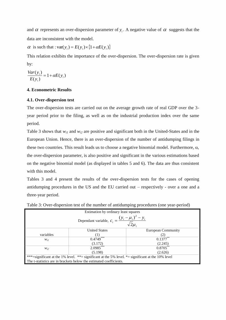
Table 3 shows that wi1 and wi2 are positive and significant both in the United-States and in the
European Union. Hence, there is an over-dispersion of the number of antidumping filings in
these two countries. This result leads us to choose a negative binomial model. Furthermore,
the over-dispersion parameter, is also positive and significant in the various estimations based
on the negative binomial model (as displayed in tables 5 and 6). The data are thus consistent
with this model.
Tables 3 and 4 present the results of the over-dispersion tests for the cases of opening
antidumping procedures in the US and the EU carried out – respectively - over a one and a
three-year period.
Table 3: Over-dispersion test of the number of antidumping procedures (one year-period)
Estimation by ordinary least squares
Dependant variable,
i
iii
i
yyc
2
)( 2
variables
United States
(1)
European Community
(2)
wi1 0.4749***
(3.172)
0.1377**
(2.245)
wi2 2.0985***
(5.198)
0.8705**
(2.626)
***=significant at the 1% level. **= significant at the 5% level. *= significant at the 10% level
The t-statistics are in brackets below the estimated coefficients.
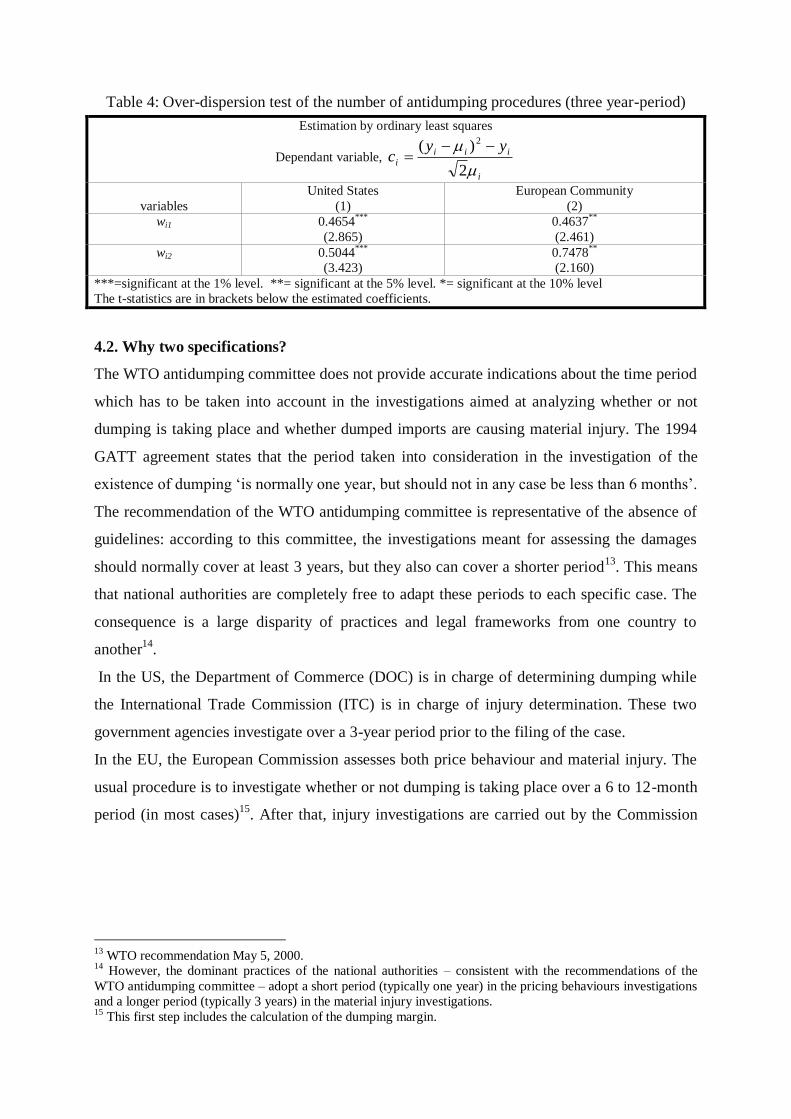
Table 4: Over-dispersion test of the number of antidumping procedures (three year-period)
Estimation by ordinary least squares
Dependant variable,
i
iii
i
yyc
2
)( 2
variables
United States
(1)
European Community
(2)
wi1 0.4654***
(2.865)
0.4637**
(2.461)
wi2 0.5044***
(3.423)
0.7478**
(2.160)
***=significant at the 1% level. **= significant at the 5% level. *= significant at the 10% level
The t-statistics are in brackets below the estimated coefficients.
4.2. Why two specifications?
The WTO antidumping committee does not provide accurate indications about the time period
which has to be taken into account in the investigations aimed at analyzing whether or not
dumping is taking place and whether dumped imports are causing material injury. The 1994
GATT agreement states that the period taken into consideration in the investigation of the
existence of dumping „is normally one year, but should not in any case be less than 6 months‟.
The recommendation of the WTO antidumping committee is representative of the absence of
guidelines: according to this committee, the investigations meant for assessing the damages
should normally cover at least 3 years, but they also can cover a shorter period13
. This means
that national authorities are completely free to adapt these periods to each specific case. The
consequence is a large disparity of practices and legal frameworks from one country to
another14
.
In the US, the Department of Commerce (DOC) is in charge of determining dumping while
the International Trade Commission (ITC) is in charge of injury determination. These two
government agencies investigate over a 3-year period prior to the filing of the case.
In the EU, the European Commission assesses both price behaviour and material injury. The
usual procedure is to investigate whether or not dumping is taking place over a 6 to 12-month
period (in most cases)15
. After that, injury investigations are carried out by the Commission
13
WTO recommendation May 5, 2000. 14
However, the dominant practices of the national authorities – consistent with the recommendations of the
WTO antidumping committee – adopt a short period (typically one year) in the pricing behaviours investigations
and a longer period (typically 3 years) in the material injury investigations. 15
This first step includes the calculation of the dumping margin.
over a 3-year period16
. However, in some cases, the time period applied to injury
determination can be reduced to only one year17
.
Of course, the choice of one year instead of 3 years in injury assessment influences the
identification of the determinants of antidumping filings. The choice of time period is an
important specification issue. Assuredly, any choice is, to some extent, arbitrary. However,
our 2 specifications (respectively based on a one-year period and a 3 three period) give a
plausible approximation of the actual procedures of the reporting countries. In addition, this
choice may be useful to differentiate the practices of the US and the EU. Lastly, it is also
justified by the fact that Knetter and Prusa (2002) and Feinberg (2003) consider a one year lag
for the foreign exchange rate and a 3-year period for the GDP, which will facilitate the
comparison between their results and ours.
Due to the correlations among the growth rate of the GDP, the rate of import penetration and
the index of industrial production, we develop three estimation models in which each of these
variables is considered separately. These models are applied, for each specification (one or
three years), both to the US and the EU, resulting in a total of 5 models to be estimated for
each country18
.
In specification #1, we consider the real GDP growth rate, the average rate of import
penetration and the industrial production index during the year prior to the antidumping filing
(see columns i, ii, and iii in tables 5 and 6).
In specification #2, we refer to these same variables over a 3-year period prior to the filing
(see columns iv, v and vi in these same tables). The real exchange rate is present in all the
specifications.
After estimating the influence of each variable on the number of filings, we try to estimate
eventual trend effects: does this influence change over time and if so in which direction?
To this end, we identify a variable, TIME, defined as the date of the filing, expressed in
number of quarters since the beginning of the period chosen (that is: since the beginning of
1990). So, the TIME value associated with the first quarter of 1990 is equal to 1, the second
quarter has a TIME value equal to 2, etc., up to 52 for the last quarter of 2002.
We capture a possible interaction between each determinant variable and TIME by
multiplying each variable by the log of TIME (Log-TIME). In order to simplify the
16
In accordance with the WTO antidumping code, a causality relation must be established between dumping and
injury to community industry. 17
See the WTO recommendation, G/ADP/6, May 16, 2000. 18
We do not take into account the value of the EU import penetration rate because we have strong doubts about
the import data extracted from the OECD database. We tried to use the data in the regressions, but the estimated
values give us erroneous coefficients.
interpretation of the estimated coefficients, we combine Log-TIME with the log of each
determinant variable, except for the GDP real growth rate (which can be a negative value).
4.3. Results
To facilitate the comparison of our results with those of Knetter and Prusa (2002) and
Feinberg (2003), we present in Tables 5 and 6 the incidence rate ratios (IRR) associated with
the estimated coefficients. The Poisson regression model assumes that the incidence rate (i.e.
the rate per unit at which a happening occurs) is a function of some underlying variables as
follows:
0 1 1 2 2 ...j j k kjx x xIr e
The expected number of occurrences is equal to this incidence rate multiplied by the exposure
(the number of units of time over which observations are measured). The exposure is
uninteresting in our case since each observation in the data set is the number of antidumping
filings in a 1-year and 3-year interval
The IRR is a function of some underlying variables. IRR represents the ratio of (1) the counts
predicted by the model when the variable of interest is one unit above its mean value and all
other variables are at their means to (2) the count predicted when all variables are at their
means also. Thus, if the IRR for the real exchange rate is 1.50, then a one unit increase in the
real exchange rate (a 100% real appreciation given that we use the log of the real rate) would
increase counts by 50% when all other variables are at their means. (Knetter and Prusa, 2003).
The t-statistics are reported for a test of the null hypothesis that the IRR=1, which would
imply no relationship between the dependant variable and the regressor.
Tables A1 and A2 summarize the results of the negative binomial model. The coefficients
generally have the expected signs. The chi-squared values obtained are high. Consequently,
the tests of the likelihood ratios confirm the global significance of the models for the United
States and the European Union.
For the United States, the estimations are completed by estimations with temporal effect
which take into account the interactions of three variables TXPIB (-1), LogTPIMP (-1) and
LogINDEXPROD (-1) with LogTIME. For the European Union, we present the specifications
without temporal effects because variables with temporal effects yield insignificant
coefficients.
4.3.1. US Results
4.3.1.1. Specification #1
The IRR estimated for the exchange rate delayed one year LogTCR (-1) is 1.03 in columns
(i), ii) and iii) of the table 5. That means a real appreciation of 100 % of the exchange rate
would increase the openings of AD procedures to 3%. The integration of the temporal effect
shows that a real appreciation of 100 % of the exchange rate delayed one year would reduce
the number of AD procedure from 11 % to 12 % (the IRR is included between 0.88 and 0.86).
The average rates of GDP growth, and import penetration and the index of industrial
production are not significant. Their effects are thus considered as null, the IRR is fixed to 1.
When we take into account the temporal effect, the IRR of LogTIME*TXPIB (-1) is 0.78,
implying that a 22 % reduction in the number of openings of procedures is associated to an
increase of 1 % of the GDP growth rate with temporal effect. The IRR of LogTIME*TPIMP
(-1) is 0.31. An increase of 100 % of the import penetration rate of the United States would
increase the number of openings of antidumping procedures to 69 % in the time period
considered. Finally, the IRR of LogTIME*INDEXPROD (-1) is 1.08. An increase of 100 %
of the index of industrial production would lead to an increase of 8 % of the number of
openings antidumping procedures.
On the whole, our results show that short variations in the level of general economic activity
or in the level of industrial activity or in imports have no significant impact on the number of
openings of antidumping procedures. Next we consider the results for longer periods.
4.3.1.2. Specification #2
Columns (iv), (v) and (vi) in Table 5 show that an appreciation of 100 % in the lagged real
exchange rate would increase openings of antidumping procedures by 25 %. An appreciation
of 100 % in the lagged real exchange rate with temporal effect LogTIME*LogTCR (-1)
would reduce the number of procedures by 27 %. The directions of evolution of variables are
coherent with those obtained by Feinberg (2003). It means that the positive relation between
the real exchange rate and the opening of antidumping inquiry is a short term relation. Over a
long period, the appreciation of the exchange rate would even tend to lower the number of AD
procedures.
The IRR of the average GDP growth rate XCDP(-3) is 0.09. A decline of a unity of the
growth rate would thus increase the number of openings of antidumping procedures by 91 %
in the United States. This result confirms our expectations and is in accordance with the
results of the previous studies: the slowing down and, to an even greater extent, the decline of
the economic activity increase the openings of antidumping actions. In the phases of
expansion, we note fewer antidumping procedures. In addition, LogTIME*XGDP(-3) does
not have a significant effect. So in the long run, there would be no direct relation between the
decline of the growth rate of the GDP and the increase in the number of antidumping
procedures. In other words, the growth rate of the GDP can influence the opening of the
procedures but only in the short-term.
It is different when we take into account the index of industrial production. Indeed, the IRR of
LogINDEXPROD (-3) is not significant. On the other hand, the IRR of
LogTIME*LogINDEXPROD (-3) is 1.02. In the long run, an increase of the index of
industrial production would thus engender an increase of 2 % in the number of antidumping
procedures in the United States.
Import penetration rate has a IRR which is practically null. An increase of 100 % of the
import penetration rate would lead to an increase of 100 % of the number of procedures. This
effect disappears in the long run (coefficient not significant for LogTIME*LogTPIMP (-3).
This means that in the long run, the intensity of the foreign competition does not produce a
significant effect on the initiations of antidumping actions. The influence of the competition is
essentially cyclic.

Table 5.IRR in the United States
Variables
Specification#1 :
Specification#2
(i) (ii) (iii) (iv) (v) (vi)
LogRER(-1)
LogTIME* LogRER(-1)
RGDP(-1)
LogTIME* RGDP(-1)
LogRIMP(-1)
LogTIME* LogRIMP(-1)
LogINDPROD(-1)
LogTIME*LogINDPROD(-1)
RGDP(-3)
LogTIME* RGDP(-3)
LogRIMP(-3)
LogTIME* LogRIMP(-3)
LogINDPROD(-3)
LogTIME*LogINDPROD(-3)
1.0303
(2.749)
0.8770
(-2.945)
1.00
(0.268)
0.7815
(-2.417)
1.0296
(2.486)
0.8763
(-2.737)
1.00
(0,858)
0,3117
(1,649)
1.0336
(2.897)
0.8652
(-3.042)
1.2719
(-3.098)
1.00
(2.952)
1.2458
(2.921)
0.7354
(-3.388)
0.0891
(-2.298)
1.2465
(2.108)
1.2511
(3.107)
0.7308
(-3.566)
1.6E-05
(1.981)
1,00
(1.052)
1.2533
(3.123)
0.7327
(-3.520)
1.00
(-0.844)
1.0179
(1.667)
4.3.2. EU Results
4.3.2.1. Specification #1
Columns (i) and (ii) in Table 6 show that the IRR of the real exchange rate lagged one year is
1.02. So, an appreciation of 100 % of the real exchange rate would increase the number of the
antidumping procedures to 2 %.
The average rate of GDP growth during the year previous to the opening of the antidumping
procedure is not significant. Short term variations in general economic activity thus do not
seem to affect the openings of antidumping inquiries in Europe.
This conclusion is qualified by the effect of the index of industrial production. Indeed, an
increase of 100 % of LogINDEXPROD (-1) would increase the number of opening
procedures by 14 % (because the IRR of the index of the industrial production is 0.856) in
Europe.
All in all only, short term variations in the branch of industry have a significant influence.
4.3.2.2. Specification #2
The real exchange rate always appears as a significant determinant of antidumping actions.
According to our estimation, an appreciation of 100 % in the real exchange rate would lead to
an increase in the number of the antidumping procedures from 13 % to 24 % (The IRR varies
between 1.13 and 1.24).
The average rate of growth during the three years which precede the opening of a procedure
has a negative coefficient but is not significant. Cyclical variations thus seem to have hardly
any influence on the openings of inquiries in Europe. This result is in accordance with what
actually happens in Europe. On the other hand, the IRR of LogINDPROD (3) is 0.796. So, an
increase of 100 % in the index of industrial production would reduce the number of anti-
dumping procedures to 20 %.
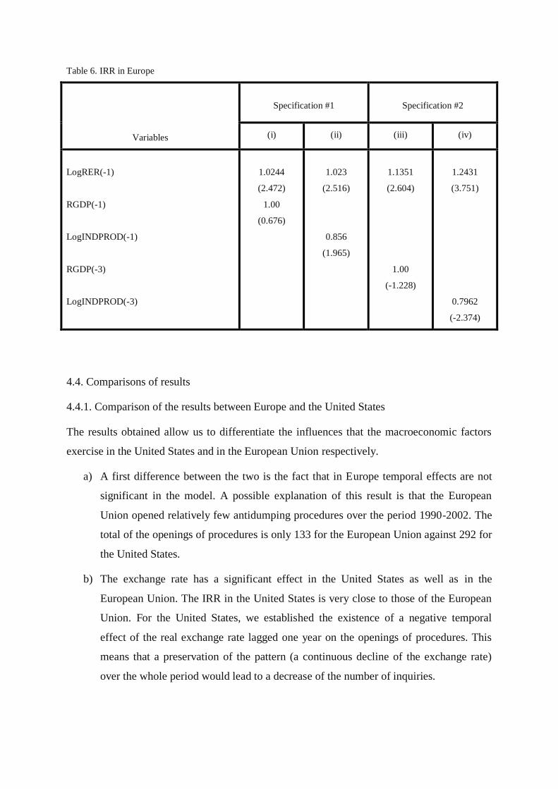
Table 6. IRR in Europe
Variables
Specification #1
Specification #2
(i) (ii) (iii) (iv)
LogRER(-1)
RGDP(-1)
LogINDPROD(-1)
RGDP(-3)
LogINDPROD(-3)
1.0244
(2.472)
1.00
(0.676)
1.023
(2.516)
0.856
(1.965)
1.1351
(2.604)
1.00
(-1.228)
1.2431
(3.751)
0.7962
(-2.374)
4.4. Comparisons of results
4.4.1. Comparison of the results between Europe and the United States
The results obtained allow us to differentiate the influences that the macroeconomic factors
exercise in the United States and in the European Union respectively.
a) A first difference between the two is the fact that in Europe temporal effects are not
significant in the model. A possible explanation of this result is that the European
Union opened relatively few antidumping procedures over the period 1990-2002. The
total of the openings of procedures is only 133 for the European Union against 292 for
the United States.
b) The exchange rate has a significant effect in the United States as well as in the
European Union. The IRR in the United States is very close to those of the European
Union. For the United States, we established the existence of a negative temporal
effect of the real exchange rate lagged one year on the openings of procedures. This
means that a preservation of the pattern (a continuous decline of the exchange rate)
over the whole period would lead to a decrease of the number of inquiries.
c) We can also note that the period used to estimate damages has a rather significant
effect on the probability of an inquiry being opened. Thus, in Europe, when a period
of one year is used to estimate the damage, the level of the IRR of the real exchange
rate is around 2 % while it is around 24 % when a 3-year period is used. In the United
States, when a period of 1 year is used to estimate the damage, we obtain an IRR from
the real exchange rate of about 3 %. The IRR is around 25 % when a 3-year period is
used. However, when the period of evaluation is of 1 year, the growth rate of the GDP
is not significant in either Europe or the United States. A contrario, when we use a
period of 3 years to estimate the damages, the GDP growth rate has a significant effect
with a weak IRR in the United States. This is not the case in Europe.
The influence of the differences in practices and the differences in the antidumping
legislation thus appear clearly. Indeed, in the United States, contrary to Europe, the I.T.C.
systematically uses a three-year period to determine the possible damage.
d) The effect of intensification of international competition is null on a horizon of 1 year
but very high in the United States on a three-year horizon. This effect is captured by
the import penetration rate variable.
e) Finally, the evolution of industrial production does explain antidumping petitions
when the period of evaluation of the damages is 3 years in the United States. On the
other hand, when we use a lag of 1 year to estimate damages, the impact of industrial
production is significant. In Europe, we obtain opposite significant effects of industrial
production when we use periods of one or three years to estimate the damages.
Overall, three main conclusions can be drawn from this comparison:
- Variations in the exchange rate are the best common explanation for both countries.
- it The index of industrial production is a good "candidate" to characterize the
European Union because is significant in Europe when the period for damage
assessment is taken as being 1 year (as is the actual practice of the European
Commission). However, the growth rate of the GDP only has a significant effect in the
United States when we use a period of 3 years to estimate the damages (as is the actual
practice of the American authorities).
- The choice of the period for the evaluation of the damages directly influences the
estimate of the probability of an inquiry being opened.
So the differences noted between the United States and Europe could be explained by the
differences of rules and practices implemented by the authorities of regulation. This is a result
not found in any of the former studies.
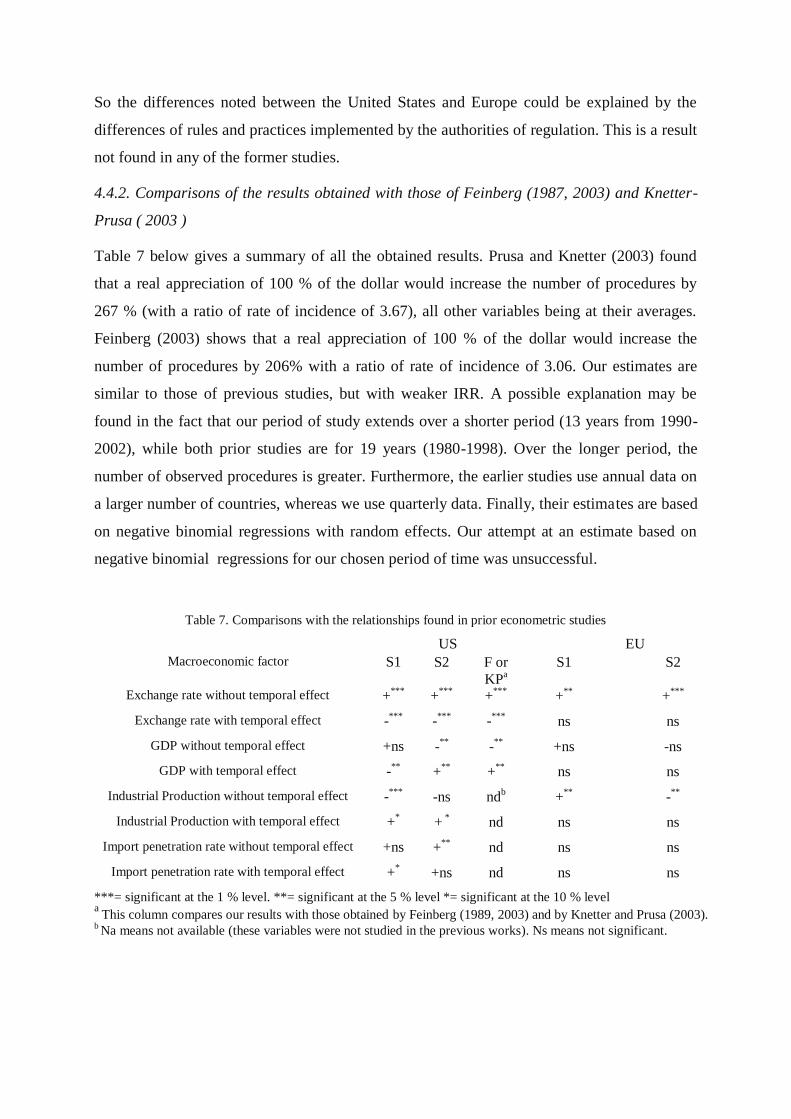
4.4.2. Comparisons of the results obtained with those of Feinberg (1987, 2003) and Knetter-
Prusa ( 2003 )
Table 7 below gives a summary of all the obtained results. Prusa and Knetter (2003) found
that a real appreciation of 100 % of the dollar would increase the number of procedures by
267 % (with a ratio of rate of incidence of 3.67), all other variables being at their averages.
Feinberg (2003) shows that a real appreciation of 100 % of the dollar would increase the
number of procedures by 206% with a ratio of rate of incidence of 3.06. Our estimates are
similar to those of previous studies, but with weaker IRR. A possible explanation may be
found in the fact that our period of study extends over a shorter period (13 years from 1990-
2002), while both prior studies are for 19 years (1980-1998). Over the longer period, the
number of observed procedures is greater. Furthermore, the earlier studies use annual data on
a larger number of countries, whereas we use quarterly data. Finally, their estimates are based
on negative binomial regressions with random effects. Our attempt at an estimate based on
negative binomial regressions for our chosen period of time was unsuccessful.
Table 7. Comparisons with the relationships found in prior econometric studies
US EU
Macroeconomic factor S1 S2 F or
KPa
S1 S2
Exchange rate without temporal effect +***
+***
+***
+**
+***
Exchange rate with temporal effect -***
-***
-***
ns ns
GDP without temporal effect +ns
-**
-**
+ns
-ns
GDP with temporal effect -**
+**
+**
ns ns
Industrial Production without temporal effect -***
-ns
ndb +
** -
**
Industrial Production with temporal effect +* +
* nd ns ns
Import penetration rate without temporal effect +ns
+**
nd ns ns
Import penetration rate with temporal effect +* +ns
nd ns ns
***= significant at the 1 % level. **= significant at the 5 % level *= significant at the 10 % level a
This column compares our results with those obtained by Feinberg (1989, 2003) and by Knetter and Prusa (2003). b Na means not available (these variables were not studied in the previous works). Ns means not significant.
5-CONCLUSION
We have shown that macroeconomic variables have different effects on the numbers of
openings of antidumping procedures in the United States and in Europe. First, an appreciation
of the real exchange rate has a positive impact on openings of procedures in the United States
and within the European Union. However, the dimension of the effect is much more important
in the United States and the temporal effect of the exchange rate is present only in the United
States. Next, the economic cycle (measured by GDP changes) has an impact on openings of
procedures only in the United States. The intensification of foreign competition (measured by
the import penetration rate) also increases openings of procedures in the United States.
Openings are also influenced by the the very short term and\or medium-term level of general
American economic activity, whereas they depend more specifically on the economic
situation of the industry in Europe. These results show the influence of institutional
differences, notably in the rules which prevail for the antidumping procedures on both sides of
the Atlantic. The difference concerning the reference periods in the calculation of damages is
perceptible in our results (a shorter period in the case of the European Union of the order of
15 months against 3 years in the United States). It also seems that the European procedure is
less effective – or, at least, offers a lesser degree of protection - than the American procedure
when we consider the impact of the economic cycle, the influence of exchange rates and
competitive pressures. Paradoxically, however, the European procedure seems more selective,
perhaps more targeted, than the American procedure (we noted no significant relationship
with the GDP in Europe, but a relationship with industrial production was found in Europe
whereas the opposite was found for the United States). Future research should go beyond the
simple explanation of openings of antidumping procedures undertaken in this study to take
into account the impact of world competition. Also the impact of the definition of dumping in
the WTO Agreements, which does not mention that the appreciation of the exchange rate can
justify the opening of an antidumping inquiry, needs to be explored. For example, only cases
of dumping which lead to a threat of monopolization of the market must now be sanctioned in
the form of temporary or definitive antidumping rights. These two factors, world competition
and the WTO definition of dumping may be found to have major responsibility for the current
intensification of the use of non-tariff barriers, in particular institutional barriers to exchanges.
This crawling neo-protectionism (Sandretto,1998) could eventually ruin the efforts of half a
century to liberalize international exchanges and build a multilateral commercial system. The
European Union and the United States should accept the responsibility for engaging in a
“disarmament” process regarding these procedures by proposing an amendment to the
Antidumping Agreement which would limit the discretionary power of the national
authorities. It would also be advisable to increase transparency in the determination of
damage, in the normal calculation of the value of damage, and in the determination of the
dumping margin (Aussilloux, 2002).
References
Aussilloux V. (2001), « Une révision souhaitable de la procédure antidumping à l‟OMC »,
Revue Française d’économie, Volume XV, avril.
Aussilloux V., Kobak, J., Sadni-Jallab M., (2004), „Antidumping as anticompetitive practices,
evidence from the United States and the European Community‟. Mimeo.
Anderson J.E. (1992), „Domino Dumping I: Competitive Exporters‟. American Economic
Review. Vol. 82, pp. 65-83.
Anderson, James E. (1993), „Domino Dumping II: Anti-dumping‟. Journal of International
Economics. Vol. 35, pp. 133-150.
Baldwin R.E. and Steagall J.W. (1994), „An Analysis of ITC Decisions in Antidumping,
Countervailing Duty and Safeguard Cases‟. Weltwirtschaftliches Archiv, Vol. 130(2),
pp. 290-308.
Blonigen B.A., Michael P. Gallaway and Flynn Joseph E. (1999), „Welfare Costs of the U.S.
Antidumping and Countervailing Duty Laws‟. Journal of International Economics, Vol. 49,
pp.211-244.
Blonigen B.A. and E. Haynes S. (2002), „Antidumping Investigations and the Pass-Through
of Exchange rates and Antidumping Duties‟. American Economic Review, Vol. 92,
pp.1044-1061.
Blonigen B., and Prusa T.J., „Antidumping‟. In: E. Kwan Choi and J. Harrigan (Eds),
Handbook of International trade. Oxford, UK, and Cambridge, MA: Blackwell Publishers,
forthcoming.
Bown C.P. and Blonigen B.A., (2003), „Antidumping and retaliation threats‟. Journal of
International Economics, Vol. 60, pp.249-273.
Cameron A. et Trivedi P., (1986), „Econometric Models Based on Count Data: Comparisons
and Applications of some Estimators and Tests‟. Journal of Applied Econometrics, Vol 1,
pp. 29-54.
Cameron A. et Trivedi P.(1990), „Regression Based Tests for Overdipersion in the Model
Poisson‟. Journal of Econometrics, Vol. 46, pp. 347-364.
Cumby R.E. and Moran T.H. (1997), „Testing Models of the Trade Policy Process:
Antidumping and the “New Issues”‟. In: Robert C. Feenstra (Ed.), The Effects of U.S. Trade

Protection and Promotion Policies. Chicago: University of Chicago Press for National
Bureau of Economic Research, pp. 161-190.
Feinberg R. (1989), „Exchange Rate and Unfair Trade‟. The Review of Economics and
Statistics, Vol. 71(4), pp.704-707.
Feinberg R. (2003), „Exchange Rates and U.S. Dumping Petitions Revisited: Does Commerce
Matter?‟. Mimeo
Hansen W.L. and Prusa T.J. (1996), „Cumulation and ITC Decision Making: The Sum of the
Parts is Greater than the Whole‟. Economic Inquiry, Vol. 34(4), pp. 746-769.
Hansen W.L. and Prusa T.J. (1997), „The Economics and Politics of Trade Policy: An
Empirical Analysis of ITC Decision Making‟. Review of International Economics, Vol. 5(2),
pp. 230-245.
Hausman J, Hall B., Griliches Z. (1984), „Economic Models for Count Data with an
Application to the Patents-R&D‟? Econometrica, vol.(52), pp 909-938.
Herander M.G. and Schwartz J.-B. (1984), „An Empirical Test of the Impact of the Threat of
U.S. Trade Policy: The Case of Antidumping Duties‟. Southern Economic Journal, July,
Vol. 51(1), pp. 59-79.
Knetter M.M. and Prusa T.J. (2003), „Macroeconomic Factors and Anti-Dumping Filings:
Evidence from Four Countries‟. Journal of International Economics. Vol. 61 (1), pp. 1-17.
Maur J.-C. (1998), „Echoing Antidumping Cases: Regulatory Competitors, Imitation and
Cascading Protection‟. World Competition, Vol. 21(6), pp 51-84.
Moore M.O. (1992), „Rules or Politics? An Empirical Analysis of ITC Anti-dumping
Decisions‟. Economic Inquiry, July, Vol. 30(3), pp. 449-466.
Prusa T.J. (1992), „Why Are So Many Antidumping Petitions Withdrawn?‟. Journal of
International Economics. Vol. 33, pp. 1-20.
Prusa T.J. (1994), „Pricing Behavior in the presence of antidumping law‟. Journal of
Economics. Vol 33, pp. 1-20.
Prusa T.J. (1997), „The Trade effects of US antidumping actions‟. In: Effects of U.S. Trade
Protection and Promotion Policies, in: Robert C. Feenstra ed, (University of Chicago Press,
Chicago).
Sadni-Jallab M. (2004), « La dimension stratégique de l‟antidumping : Analyse théorique et
empirique pour les Communautés Européennes et les États-Unis pour la période 1990-2002 »,
Thèse de Doctorat, Université Lumière Lyon 2.
Sandretto R. (1998), « Le protectionnisme au tournant du siècle : opacité et furtivité ». Études
Internationales. Institut québécois des hautes études Internationales, Vol XXIX, n° 2, juin.
Shin H.J. (1995), « Caractéristiques des actions antidumping aux États-Unis Durant la
décennie 1980 ». In : OCDE : Politique de la concurrence dans les pays de l’OCDE, 638 p.
Shin H.J. (1998), „Possible instances of Predatory Pricing in recent U.S. Antidumping Cases‟.
In: Antidumping: What does the Evidence Show? Brookings Trade Forum, Brookings
Institution Press.
Willig R.D. (1998), “Economic Effects of Antidumping Policy”. In: Antidumping: What does
the Evidence Show? Brookings Trade Forum, Brookings Institution Press.
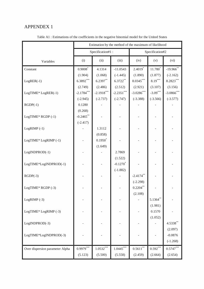
APPENDEX 1
Table A1 : Estimations of the coefficients in the negative binomial model for the United States
Variables
Estimation by the method of the maximum of likelihood
Specification#1 : Specification#2
(i) (ii) (iii) (iv) (v) (vi)
Constant
LogRER(-1)
LogTIME* LogRER(-1)
RGDP(-1)
LogTIME* RGDP (-1)
LogRIMP (-1)
LogTIME* LogRIMP (-1)
LogINDPROD(-1)
LogTIME*LogINDPROD(-1)
RGDP(-3)
LogTIME* RGDP (-3)
LogRIMP (-3)
LogTIME* LogRIMP (-3)
LogINDPROD(-3)
LogTIME*LogINDPROD(-3)
0.9008*
(1.904)
6.3892***
(2.749)
-2.1784***
(-2.945)
0.1280
(0.268)
-0.2465**
(-2.417)
-
-
-
-
-
-
-
-
-
-
4.1314
(1.068)
6.2397**
(2.486)
-2.1918***
(-2.737)
-
-
1.3112
(0.858)
0.1950*
(1.649)
-
-
-
-
-
-
-
-
-11.0543
(-1.445)
6.3722**
(2.512)
-2.2351***
(-2.747)
-
-
-
-
2.7869
(1.522)
-0.1270*
(-1.882)
-
-
-
-
-
-
2.4019*
(1.890)
8.0345***
(2.921)
-3.0286***
(-3.388)
-
-
-
-
-
-
-2.4174**
(-2.298)
0.2204**
(2.108)
-
-
-
-
11.780*
(1.877)
8.19***
(3.107)
-3.09***
(-3.566)
-
-
-
-
-
-
-
-
5.1364**
(1.981)
0.1570
(1.052)
-
-
-19.966**
(-2.162)
8.2823***
(3.156)
-3.0866***
(-3.577)
-
-
-
-
-
-
-
-
-
-
4.5338**
(2.097)
-0.0876
(-1.268)
Over dispersion parameter Alpha 0.9979***
(5.123)
1.0532***
(5.500)
1.0445***
(5.558)
0.5611**
(2.459)
0.592***
(2.664)
0.5747***
(2.654)

Log likelihood unrestricted. L0
Log likelihood restricted. Lr
Chi-squareda
Significance level
Number of observations
Degrees freedom
-316.3238
-364.5566
96.46556
0.0000
220
1
-318.5656
-369.3118
101.4925
0.0000
220
1
-317.9812
-368.3517
100.7409
0.0000
220
1
-236.2167
-245.2801
18.1267
0.207E-04
180
1
-236.63
-247.14
21.0202
0.4E-05
180
1
-245.7997
-263.9425
36.2856
0.0000
180
4
a- 2
02 ( ) ( )rLog L Log L
***=significant at the 1 % level. **= significant at the 5 % level. *= significant at the 10 % level.
The t-statistics are in brackets below the estimated coefficients.
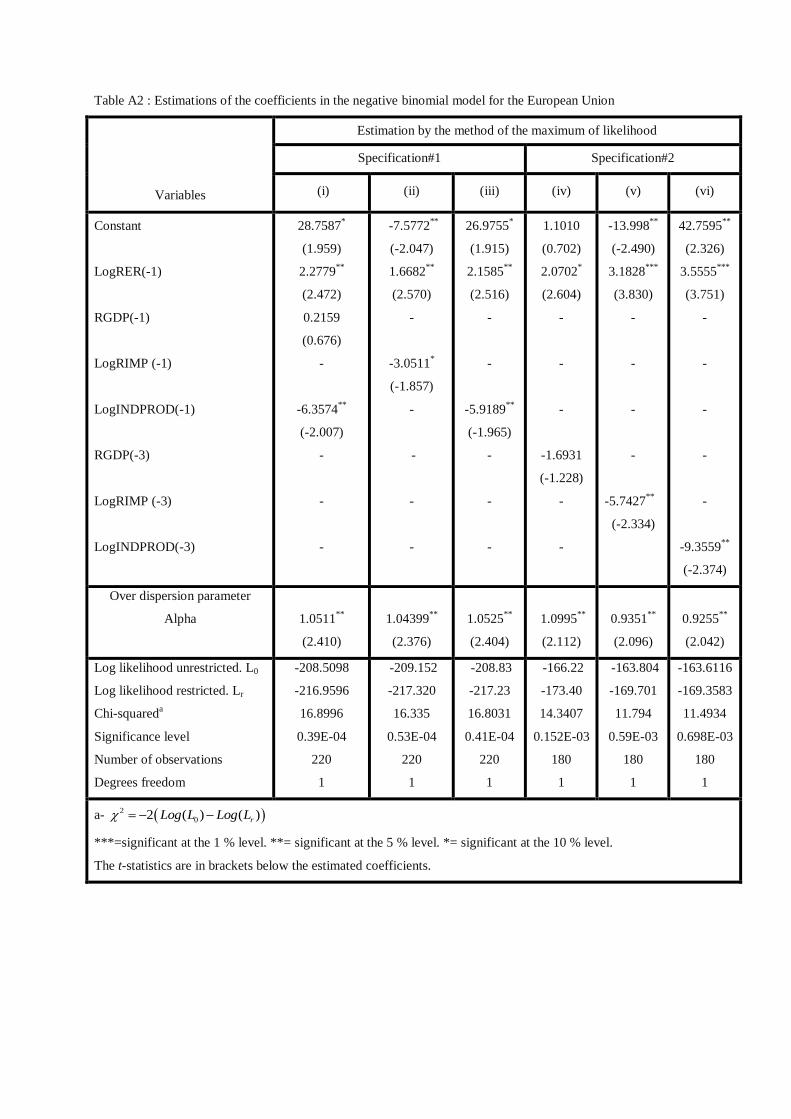
Table A2 : Estimations of the coefficients in the negative binomial model for the European Union
Variables
Estimation by the method of the maximum of likelihood
Specification#1 Specification#2
(i) (ii) (iii) (iv) (v) (vi)
Constant
LogRER(-1)
RGDP(-1)
LogRIMP (-1)
LogINDPROD(-1)
RGDP(-3)
LogRIMP (-3)
LogINDPROD(-3)
28.7587*
(1.959)
2.2779**
(2.472)
0.2159
(0.676)
-
-6.3574**
(-2.007)
-
-
-
-7.5772**
(-2.047)
1.6682**
(2.570)
-
-3.0511*
(-1.857)
-
-
-
-
26.9755*
(1.915)
2.1585**
(2.516)
-
-
-5.9189**
(-1.965)
-
-
-
1.1010
(0.702)
2.0702*
(2.604)
-
-
-
-1.6931
(-1.228)
-
-
-13.998**
(-2.490)
3.1828***
(3.830)
-
-
-
-
-5.7427**
(-2.334)
42.7595**
(2.326)
3.5555***
(3.751)
-
-
-
-
-
-9.3559**
(-2.374)
Over dispersion parameter
Alpha
1.0511**
(2.410)
1.04399**
(2.376)
1.0525**
(2.404)
1.0995**
(2.112)
0.9351**
(2.096)
0.9255**
(2.042)
Log likelihood unrestricted. L0
Log likelihood restricted. Lr
Chi-squareda
Significance level
Number of observations
Degrees freedom
-208.5098
-216.9596
16.8996
0.39E-04
220
1
-209.152
-217.320
16.335
0.53E-04
220
1
-208.83
-217.23
16.8031
0.41E-04
220
1
-166.22
-173.40
14.3407
0.152E-03
180
1
-163.804
-169.701
11.794
0.59E-03
180
1
-163.6116
-169.3583
11.4934
0.698E-03
180
1
a- 2
02 ( ) ( )rLog L Log L
***=significant at the 1 % level. **= significant at the 5 % level. *= significant at the 10 % level.
The t-statistics are in brackets below the estimated coefficients.