Zbigniew Osiak

ANTI GRAVITY-

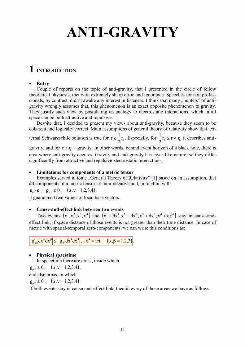
rS

0.5rS

0.5rS

GRAVITY

ANTI-GRAVITY

GRAVITY

2

Links to my popular-science and science publications, e-books and radio/TV auditions are

available in ORCID database: http://orcid.org/0000-0002-5007-306X

3

Mathematics should be a servant, not a queen.

To Margaret,

my daughter,

I dedicate

Zbigniew Osiak

ATI-GRAVITYABOUT HOW GEERAL RELATIVITY

HIDES ATI-GRAVITY – HEURISTIC APPROACH

4

Anti-gravity

by Zbigniew Osiak

e-mail: zbigniew.osiak@gmail.com

Portraits (drawings) of Newton, Gauss, Einstein and Schwarzschild – Małgorzata Osiak

Portrait of the author on back cover – Rafał Pudło

Translated by Rafał Rodziewicz

5

TABLE OF COTETS

TITLE PAGE

COPYRIGHT LAW PAGE

1 ITRODUTIO 11

• Entry 11

• Limitations for components of a metric tensor 11

• Cause-and-effect link between two events 11

• Physical spacetime 11

• Relations between components of a metric tensor and local basis vectors 12

• Dot product 12

• Vector value 13

• Physical (true) vector components 13

• Vector value expressed by physical vector components 13

• Cosine of an angle between local basis vectors 13

• Stationary metric with spatial-temporal zero-components 14

• Quoted works 14

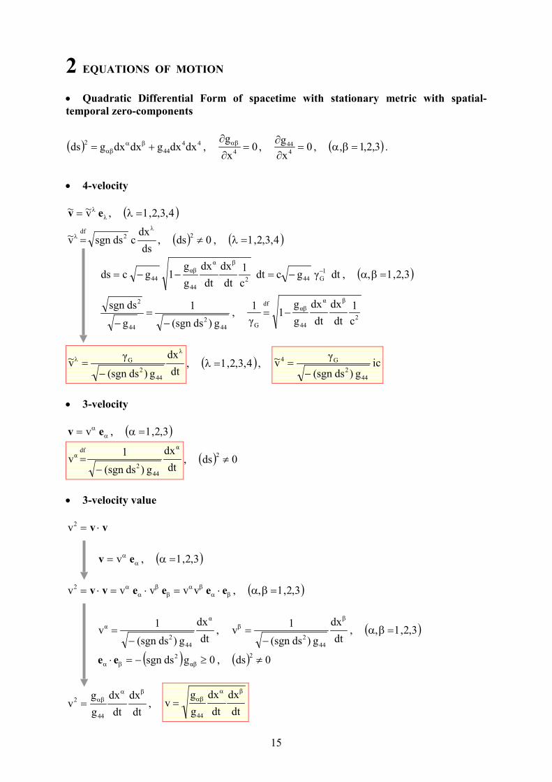
2 EQUATIOS OF MOTIO 15

• Quadratic Differential Form of spacetime with stationary metric with spatial-temporalzero-components 15

• 4-velocity 15

• 3-velocity 15

• 3-velocity value 15

• Physical (true) components of 3-vector 16

• Lorentz factor 16

• Components of 4-vector expressed by components of 3-vector 16

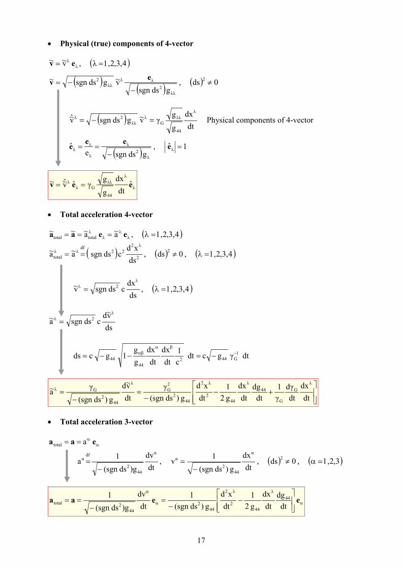
• Physical (true) components of 4-vector 17

• Total acceleration 4-vector 17

• Total acceleration 3-vector 17

• Value of total acceleration 3-vector 18

• Physical (true) components of total acceleration 3-vector 18

• Components of total acceleration 4-vector expressed by components of total acceleration

3-vector 18

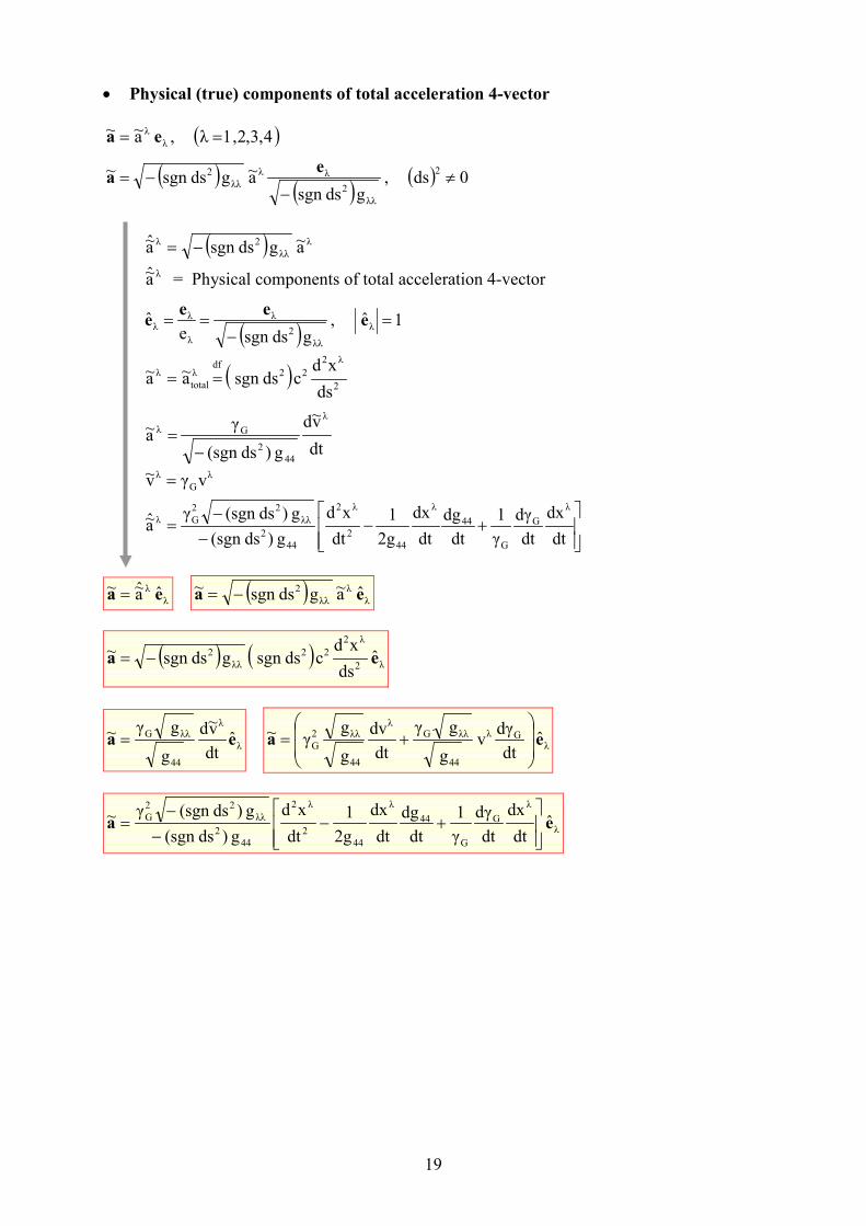
• Physical (true) components of total acceleration 4-vector 19

• 4-dimension motion equations of a test particle 20

6

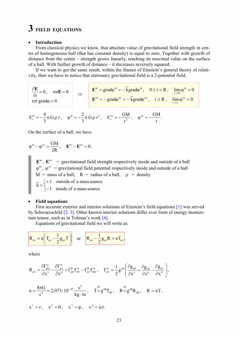
3 FIELD EQUATIOS 21

• Introduction 21

• Field equations 21

• Quoted works 22

4 GRAVITATIOAL FIELD OUTSIDE MASS SOURCE 23

• Exterior Schwarzschild metric 23

• Speed of light propagation and exterior Schwarzschild metric 23

• Gravitational acceleration of free fall outside mass source 23

• Gravity and anti-gravity 24

• Main hypothesis 25

• Quoted works 25

5 BLACK HOLE WITH MAXIMAL ATI-GRAVITY HALO

• Black hole with maximal anti-gravity halo 26

6 GRAVITATIOAL FIELD ISIDE MASS SOURCE 27

• Spacetime metric inside mass source 27

• Speed of light propagation in virtual vacuum that is inside mass source 27

• Gravitational acceleration of free fall inside mass source 28

7 GRAVITATIOAL FIELD ISIDE BLACK HOLE WITH MAXIMAL ATI-

GRAVITY HALO 29

• Spacetime metric inside black hole with maximal anti-gravity halo 29

• Speed of light propagation in virtual vacuum tunnel that is inside black hole with maximal

anti-gravity halo 29

• Gravitational acceleration of free fall inside black hole with maximal anti-gravity halo 30

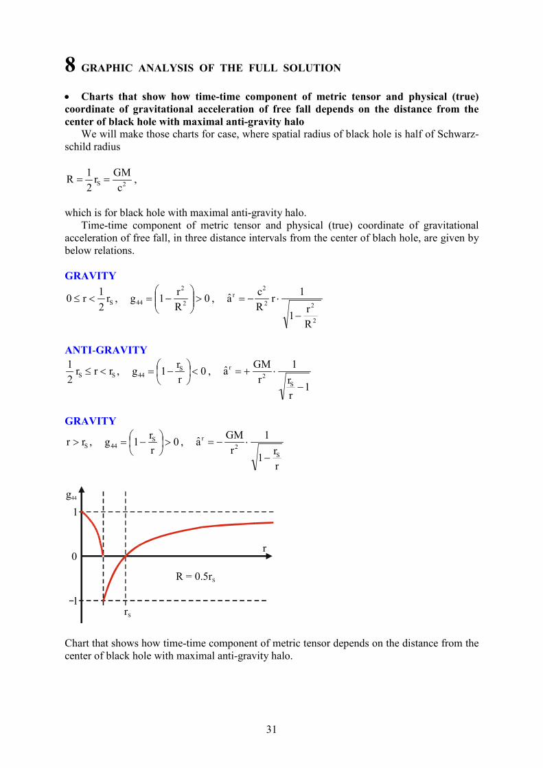
8 GRAPHIC AALYSIS OF FULL SOLUTIO 31

• Charts that show how time-time component of metric tensor and physical (true) coordi-

nate of gravitational acceleration of free fall depends on the distance from the center of

black hole with maximal anti-gravity halo 31

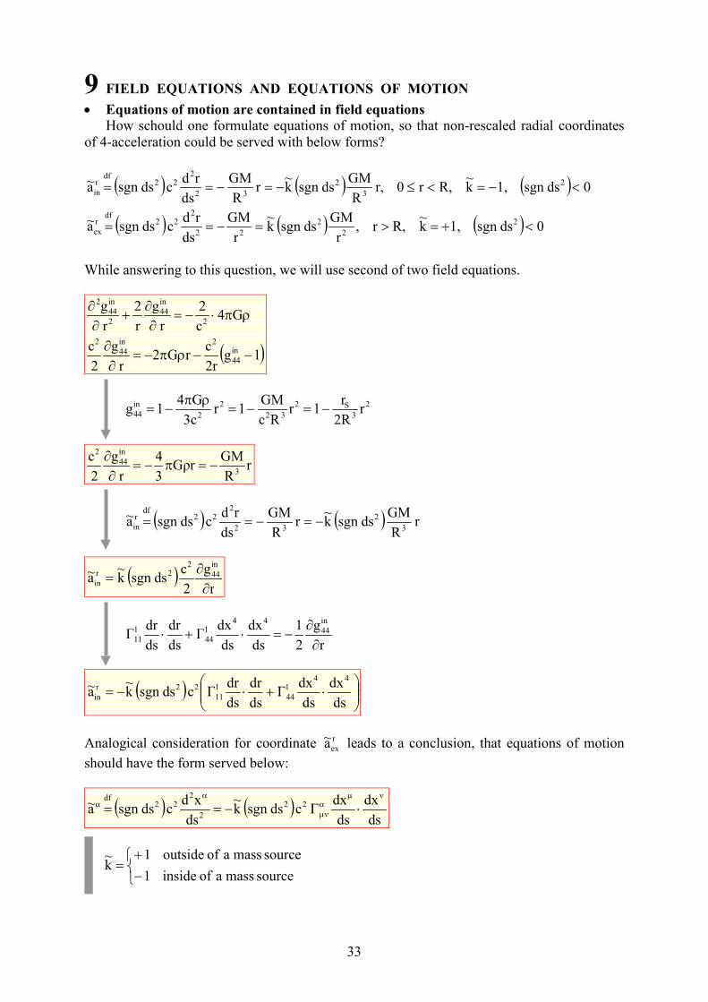
9 FIELD EQUATIOS AD EQUATIOS OF MOTIO 33

• Equations of motion are contained in field equations 33

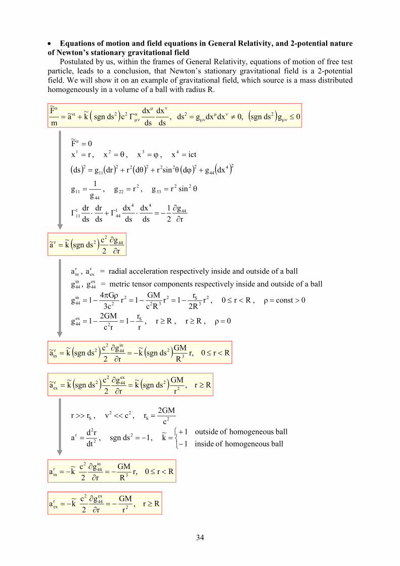
• Equations of motion and field equations in General Relativity, and 2-potential nature of

Newton’s stationary gravitational field 34

7

10 EW TEST OF GEERAL RELATIVITY 39

• The proposition of the experiment 39

11 BLACK HOLE MODEL OF OUR UIVERSE 40

• Our Universe as a black hole with maximal anti-gravity halo 40

• Radius of Our Universe 40

12 PHOTO PARADOX 41

• Introduction 41

• Gravitational redshift 41

• Conformally flat spacetime 41

• Schwarzschild spacetime 41

• Friedman-Lemaître-Robertson-Walker spacetime 41

• Photon paradox 42

• Does photons have memory? 42

• Energy of photon in Newton’s gravitational fiel 42

• Hydrogen atom in Schwarzschild gravitational field – heuristic approach 44

• How to define redshift? 44

• Redshift of light which comes to Earth from the Sun 45

• Redshift of light which comes to Earth from a distant galaxy 45

• Hubble's law 47

• Radius of Our Universe according to Hubble's observation 47

• Average density of Our Universe according to Hubble's observation 48

• Constancy of photon energy and Pound-Rebka experiment 48

• Quoted works 50

13 EARTH GRAVITATIOAL FIELD AD UIVERSE GRAVITATIOAL

FIELD 51

• Influence of gravitational field on space and time distances 51

• Local properties of redshift 51

• Conclusions 52

14 OLBERS PARADOX 53

• Olbers paradox 53

• Probability of photon hitting Earth 53

• Bohr hydrogen atom in Our Universe 53

• Illuminance of Earth surface at night 54

• Quoted works 56

8

15 MICROVAWE BACKGROUD RADIATIO 57

• Background radiation 57

• Background radiation in Big-Bang theory 57

• Background radiation in Black Hole Universe 57

• Quoted works 58

16 AVERAGE UIVERSE DESITY I FRIEDMA’S THEORY 59

• Critical density 59

• Density parameter and current average density of Friedman’s universe 59

• Dark energy 59

• Quoted works 59

17 ATI-GRAVITY I OTHER MODELS OF UIVERSE 60

• Gravitational acceleration of free particle corresponding with F-L-R-W metric 60

• Gravitational acceleration of free particle corresponding with metric of simple model of

expanding spacetime 61

• Quoted works 62

18 OUR UIVERSE AS A EISTEI’S SPACE 63

• Other form of field equations – Our Universe as an Einstein’s space 63

• Quoted works 63

19 ASSUMPTIOS 64

• Main postulates of General Relativity 64

• 2-potential nature of stationary gravitational field 64

• Poisson’s equation and 2-potential nature of stationary gravitational field 64

• Signes of right sides of Poisson’s and Einstein’s equations and boundary conditions 64

• Hypothesis about memory of photons 65

20 STABILITY OF THE MODEL 66

• Stability of the model 66

• Gravitational Gauss law and galaxies 66

21 MAI RESULTS 68

• Hypothesis about existence of anti-gravity 68

• Black hole with maximal anti-gravity halo 68

• Hypothesis about 2-potential nature of stationary gravitational field 68

9

• Field equations contain equations of motion 68

• Black Hole model of Our Universe 68

• Size of Our Universe 69

• Density of Our Universe 69

• Photon paradox 69

• Hypothesis about memory of photons 69

• Our Universe is an Einstein’s space 69

• Anti-gravity in other cosmological models 69

• New tests of General Relativity 70

• Quoted works 70

22 ADDITIO – MATHEMATICS 71

• Explicit form of Christoffel symbols of first and second kind 71

• Explicit form of covariant Ricci curvature tensor 71

• Field equations 72

• Curvature scalar 73

• Field equations expressed by curvature scalar 73

• Laplace operator (Laplacian) in Cartesian and spherical coordinate systems 75

• Used relations 75

23 ADDITIO – PHYSICS 76

• Hydrogen spectral series in Earth conditions 76

• Hydrogen spectral series in Our Universe 77

• Electromagnetic spectrum 77

• Choosen concepts, constants and units 78

24 ADDITIO – HISTORY 80

• Newton’s law of gravitation 80

• Gauss law of gravitation 80

• Einstein’s General Theory of Relativity 81

• External (vacuum) Schwarzschild solution 81

25 EDIG 82

• Author’s reflections 82

10

11

ATI-GRAVITY

1 ITRODUCTIO

• Entry Couple of reports on the topic of anti-gravity, that I presented in the circle of fellow

theoretical physicsts, met with extremely sharp critic and ignorance. Speeches for non profes-

sionals, by contrast, didn’t awake any interest in listeners. I think that many „hunters” of anti-

gravity wrongly assumes that, this phenomenon is an exact opposite phenomenon to gravity.

They justify such view by postulating an analogy to electrostatic interactions, which in all

space can be both attractive and repulsive.

Despite that, I decided to present my views about anti-gravity, because they seem to be

coherent and logically correct. Main assumptions of general theory of relativity show that, ex-

ternal Schwarzschild solution is true for Sr2

1r ≥ . Especially, for SS rrr

2

1<≤ it describes anti-

gravity, and for Srr > – gravity. In other words, behind event horizon of a black hole, there is

area where anti-gravity occures. Gravity and anti-gravity has layer-like nature, so they differ

significantly from attractive and repulsive electrostatic interactions.

• Limitations for components of a metric tensor Examples served in tome „General Theory of Relativity” [1] based on an assumption, that

all components of a metric tensor are non-negative and, in relation with

0g ≥=⋅ µννµ ee , ( )4,3,2,1, =νµ ,

it guaranteed real values of local base vectors.

• Cause-and-effect link between two events

Two events ( )4321 x,x,x,x and ( )44332211 dxx,dxx,dxx,dxx ++++ stay in cause-and-

effect link, if space distance of those events is not greater than their time distance. In case of

metric with spatial-temporal zero-components, we can write this conditions as:

( )1,2,3, ict, x, dxdxg dxdxg 444

44

βα =βα=≤αβ .

• Physical spacetime In spacetime there are areas, inside which

0g ≥µν , ( )4,3,2,1, =νµ ,

and also areas, in which

0g ≤µν , ( )4,3,2,1, =νµ .

If both events stay in cause-and-effect link, then in every of those areas we have as follows:

12

( ) ( )4,3,2,1, , 0ds , 0g2 =νµ≤≥µν

and

( ) ( )4,3,2,1, , 0ds , 0g2 =νµ≥≤µν .

Areas that fulfill above conditions, we will call physical spacetime.

In areas, inside which

0g ≥µν , ( ) 0ds2 > , ( )4,3,2,1, =νµ

or

0g ≤µν , ( ) 0ds2 < , ( )4,3,2,1, =νµ ,

there is no single pair of events that stays in cause-and-effect link.

• Relations between components of a metric tensor and local basis vectors If we want to get local basis vectors with real values in physical spacetime, then we need

to adopt new relation between those vectors and components of a metric tensor.

( ) 0g dssgn 2 ≥−=⋅ µννµ ee , ( ) 0ds2 ≠ , ( )4,3,2,1, =νµ

It causes a necessity to change a definition of dot product and associated terms. Those chan-

ges, forced by physics, will cause only small complication of some formulas.

In cases when

( ) 0ds2 < and 0g ≥µν ,

above modifications doesn’t lead to any changes, in previously quoted by Me tome titled

„General Theory of Relativity” [1].

( ) 0g dssgn 2 ≥−=⋅ µννµ ee , ( ) 0ds2 ≠ , ( )4,3,2,1, =νµ

( ) 0ds2 <

0g ≥=⋅ µννµ ee

• Dot product

Dot product of vectors µµ= eA A and ν

ν= eB A we will call phrase

νµνµ ⋅=⋅ eeBA BA

( ) 0g dssgn 2 ≥−=⋅ µννµ ee , ( ) 0ds2 ≠ , ( )4,3,2,1, =νµ

( ) νµµν−=⋅ BAg dssgn 2BA

13

• Vector value

( ) νµννµ

νµ −=⋅=⋅ AAg dssgn AA µ2eeAA , ( ) 0ds2 ≠ , ( )4,3,2,1, =νµ

( ) ν2 AAg dssgn A µµν−=⋅== AAA

• Physical (true) vector components

µµ= eA A

( )( ) µµ

µµµµ

−−=

g dssgn A g dssgn

2

2e

A , ( ) 0ds2 ≠ , ( )4,3,2,1, =νµ

( ) µ

µµ

2µ A g dssgn A −= Physical vector components

( ) µµ

2 g dssgn eˆ

−== µ

µ

µµ

eee , 1ˆ =µe

µ= eA ˆ Aµ

• Vector value expressed by physical vector components

νµνµ ⋅=⋅ eeAA A A

( ) ( ) νν

2

µµ

2

νµ

νµ

g dssgn g dssgn

AA AA

−−=

( ) 0g dssgn 2 ≥−=⋅ µννµ ee , ( ) 0ds2 ≠ , ( )4,3,2,1, =νµ

( )

( ) ( ) ννµµνν

2

µµ

2

2

gg

g

g dssgn g dssgn

g dssgn µνµν =−−

−

ννµµ

µν

νµ

gg

g AAA =⋅== AAA

• Cosine of an angle between local basis vectors

( )νµνµνµ =⋅ eeeeee , cos

( ) 0g dssgn µν

2 ≥−=⋅ νµ ee , ( ) 0ds2 ≠ , ( )4,3,2,1, =νµ

( ) 0g dssgn 2 ≥−= µµµe

( ) 0g dssgn 2 ≥−= νννe

14

( )ννµµ

µν

νµ

νµνµ =

⋅=

gg

g

, cos

ee

eeee

• Stationary metric with spatial-temporal zero-components For the sake of simplicity, let’s limit detailed contemplations to a stationary metric with

spatial-temporal zero-components, that is:

( ) 44βααβ += dxdxgdxdxgds 44

2, 0

x

g4

=∂

∂ αβ, 0

x

g4

44 =∂∂

, ( )3,2,1, =βα .

Example of such metric is external Schwarzschild metric, which depending on output coordi-

nate system, can be written in equivalent forms:

( ) 44S44

1

S

2

2dxdx

r

rdxdx 1

r

r1

r

xxds

−δ+

−

−+δ= βα

−βα

αβ , ( )3,2,1, =βα ,

ictx ,zx ,yx ,xx 4321 ==== , 2S

c

GM2r =

or

( ) 44S222222

1

S2dxdx

r

r1 d sinrdrdr

r

r1 ds

−+ϕθ+θ+

−=

−

,

ictx ,x ,x ,rx 4321 =ϕ=θ== , 2S

c

GM2r = .

Quoted works[1] Z. Osiak: Ogólna Teoria Względności (General Theory of Relativity). Self Publishing

(2012), ISBN: 978-83-272-3515-2

15

2 EQUATIOS OF MOTIO

• Quadratic Differential Form of spacetime with stationary metric with spatial-

temporal zero-components

( ) 44βααβ += dxdxgdxdxgds 44

2, 0

x

g4

=∂

∂ αβ, 0

x

g4

44 =∂∂

, ( )3,2,1, =βα .

• 4-velocity

λ

λ v~~ ev = , ( )1,2,3,4=λ

ds

dx c dssgn v~ 2

dfλ

λ = , ( ) 0ds2 ≠ , ( )1,2,3,4=λ

dt γgc dt c

1

dt

dx

dt

dx

g

g1 g cds 1

G442

βα

44

αβ

44

−−=−−= , ( )1,2,3=βα,

44

2

44

2

g )dssgn (

1

g

dssgn

−=

−,

2

βα

44

αβdf

G c

1

dt

dx

dt

dx

g

g1

γ

1−=

dt

dx

g )dssgn (

γv~

λ

44

2

G

−=λ

, ( )1,2,3,4=λ , ic g )dssgn (

γv~

44

2

G4

−=

• 3-velocity

αα= ev v , ( )1,2,3=α

dt

dx

g )dssgn (

1v

α

44

2

dfα

−= , ( ) 0ds

2 ≠

• 3-velocity value

vv ⋅=2v

αα= ev v , ( )1,2,3=α

βαβα

ββ

αα ⋅=⋅=⋅= eeeevv vv v vv2 , ( )1,2,3=βα,

dt

dx

g )dssgn (

1v

α

44

2

α

−= ,

dt

dx

g )dssgn (

1v

44

2

ββ

−= , ( )1,2,3=βα,

( ) 0g dssgn αβ

2 ≥−=⋅ βα ee , ( ) 0ds2 ≠

dt

dx

dt

dx

g

gv

44

2

βααβ= ,

dt

dx

dt

dx

g

gv

44

βααβ=

16

• Physical (true) componets of 3-vector

αα= ev v , ( )1,2,3=α

( )( ) αα

2

α

αα

2

g dssgn vg dssgn

−−= αe

v , ( ) 0ds2 ≠

( )dt

dx

g

g vg dssgn v

α

44

ααα

αα

2α =−= Physical components of 3-vector

( ) αα

2 g dssgn eˆ

−== α

α

αα

eee , 1ˆ =αe

ααα == eev ˆ

dt

dx

g

gˆ v

α

44

αα

• Lorentz factor

2

44G c

1

dt

dx

dt

dx

g

g1

βααβ−=

γ1

dt

dx

dt

dx

g

gv

44

2

βααβ= , ( )1,2,3=βα,

2

2G

c

v1

1

−

=γ

• Components of 4-vector expressed by components of 3-vector

dt

dx

g )dssgn (

γv~

λ

44

2

G

−=λ , ( )1,2,3,4=λ

dt

dx

g )dssgn (

1v

α

44

2

dfα

−= , ( )1,2,3=α

ictx4 = ,

44

2

4

44

2

df4

g )dssgn (

ic

dt

dx

g )dssgn (

1v

−=

−=

λ

G

λ vγv~ = , ( )1,2,3,4=λ

17

• Physical (true) components of 4-vector

λ

λ v~~ ev = , ( )1,2,3,4=λ

( )( ) λλ

2

λλ

λλ

2

g dssgn v~ g dssgn ~

−−=

ev , ( ) 0ds

2 ≠

( )dt

dx

g

gγv~ g dssgn v~

λ

44

λλ

G

λ

λλ

2λ =−= Physical components of 4-vector

( ) λ

2

λ

λ

λλ

g dssgn eˆ

−==

eee , 1ˆ λ =e

λ

λ

44

λλ

Gλ

λ ˆdt

dx

g

gγˆ v~~ eev ==

• Total acceleration 4-vector

λ

λ

λ

λ

totaltotal a~ a~~~ eeaa === , ( )1,2,3,4=λ

( )2

λ2

22df

λλ

totalds

xdc dssgn a~a~ == , ( ) 0ds

2 ≠ , ( )1,2,3,4=λ

ds

dx c dssgn v~ 2

λλ = , ( )1,2,3,4=λ

ds

v~d c dssgn a~ 2

λλ =

dt γgc dt c

1

dt

dx

dt

dx

g

g1 g cds 1

G442

44

44

−βα

αβ −=−−=

+−

−=

−=

dt

dx

dt

dγ

γ

1

dt

dg

dt

dx

g 2

1

dt

xd

g )dssgn (

γ

dt

v~d

g )dssgn (

γa~

λ

G

G

44

λ

44

2

λ2

44

2

2

G

λ

44

2

Gλ

• Total acceleration 3-vector

αα== eaa atotal

dt

dv

)gdssgn (

1a

α

44

2

dfα

−= ,

dt

dx

g )dssgn (

1v

α

44

2

α

−= , ( ) 0ds

2 ≠ , ( )1,2,3=α

αα

α

−

−=

−== eeaa

dt

dg

dt

dx

g 2

1

dt

xd

g )dssgn (

1

dt

dv

)gdssgn (

1 44

λ

44

2

λ2

44

2

44

2total

18

• Value of total acceleration 3-vector

aa ⋅=2a

αα= ea a , β

β a ea = , ( )1,2,3=α

βαβα

ββ

αα ⋅=⋅=⋅= eeeeaa aa a aa2 , ( )1,2,3=βα,

dt

dv

)gdssgn (

1a

α

44

2

dfα

−= ,

dt

dv

)gdssgn (

1a

β

44

2

dfβ

−= , ( )1,2,3=βα,

( ) 0g dssgn 2 ≥−=⋅ αββα ee , ( ) 0ds2 ≠

dt

dv

dt

dv

g

ga

44

2

βααβ= ,

dt

dv

dt

dv

g

ga

44

βααβ=

• Physical (true) components of total acceleration 3-vector

αα= ea a , ( )1,2,3=α

( )( ) αα

αααα

−−=

g dssgn a g dssgn

2

2 ea , ( ) 0ds

2 ≠

( )dt

dv

g

g a g dssgn a 2

α

44

ααααα

α =−= Physical components of total acceleration 3-vector

( ) αα

α

α

αα

−==

g dssgn eˆ

2

eee , 1ˆ =αe

α

α

44

ααα

α == eea ˆdt

dv

g

g ˆ a

• Components of total acceleration 4-vector expressed by components of total accelera-

tion 3-vector

( ) dt

dγ

dt

dx

g dssgn

γaγa~ G

λ

44

2

G2

G −+= αα , ( )1,2,3=α

( ) ( ) dt

dγ

dt

dx

g dssgn

γ

dt

dv

g dssgn

γa~ G

4

44

2

G

4

44

2

2

G

−+

−=4

19

• Physical (true) components of total acceleration 4-vector

λ

λ a~~ ea = , ( )1,2,3,4=λ

( )( ) λλ

2

λλ

λλ

2

g dssgn a~ g dssgn ~

−−=

ea , ( ) 0ds

2 ≠

( ) λ

λλ

2λ a~ g dssgn a~ −=

λa~ = Physical components of total acceleration 4-vector

( ) λλ

2

λ

λ

λλ

g dssgn eˆ

−==

eee , 1ˆ λ =e

( )2

λ2

22df

λ

total

λ

ds

xdc dssgn a~a~ ==

dt

v~d

g )dssgn (

γa~

λ

44

2

Gλ

−=

λ

G

λ vγv~ =

+−

−

−=

dt

dx

dt

dγ

γ

1

dt

dg

dt

dx

2g

1

dt

xd

g )dssgn (

g )dssgn (γa~

λ

G

G

44

λ

44

2

λ2

44

2

λλ

22

Gλ

λ

λ ˆ a~~ ea = ( ) λ

λ

λλ

2 ˆ a~ g dssgn ~ ea −=

( ) ( ) λ2

λ2

22

λλ

2 ˆ ds

xdc dssgn g dssgn ~ ea −=

λ

λλλG ˆ

dt

v~d

g

g γ~ ea

44

= λGλλλG

λλλ2

Gˆ

dt

dγ v

g

g γ

dt

dv

g

g γ~ ea

+=

4444

λ

λ

G

G

44

λ

44

2

λ2

44

2

λλ

22

G ˆ dt

dx

dt

dγ

γ

1

dt

dg

dt

dx

2g

1

dt

xd

g )dssgn (

g )dssgn (γ~ ea

+−

−

−=

20

• 4-dimensional motion equations of a test particle

Postulated motion equations of a test particle has interpretation as follows:

αα

α += iner&gravtotal a~

m

F~

a~

( )2

2

22

totalds

xdc dssgn a~a~

ααα ==

( )ds

dx

ds

dxk~

c dssgn a~ 22

iner&grav

νµαµν

α Γ −=

In case of stationary metric with spatial-temporal zero-components, which is metric of type:

( ) 44

44

λκ

κλ

2dxdxgdxdxgds += , 0

x

g4

κλ =∂∂

, 0x

g4

44 =∂∂

, ( )3,2,1λκ, = ,

equations of motion, inter alia, can be also written in such forms:

( ) ( )1,2,3,4=νµα,

Γ−+

γ= α

νµαµναα

ααα , ,ˆ v~v~ k

~ g dssgn

dt

v~d

g

g

m

~2

44

G eF

α

νµαµν

ααα

Γ+

γγ

+

−

−

−γ= e

Fˆ

dt

dx

dt

dx k

~

dt

dx

dt

d1

dt

dg

dt

dx

2g

1

dt

xd

g )dssgn (

g )dssgn (

m

~G

G

44

λ

44

2

λ2

44

2

22

G

Let’s remind:

dt

dx

g )dssgn (

γv~

44

2

Gdf

αα

−= ,

2

λκ

44

κλ

G c

1

dt

dx

dt

dx

g

g1−=

γ1

, ( ) αααα −= g dssgn ˆ 2ee , 1ˆ =αe

Components of acceleration 4-vector of a test particle with mass (m) in given point of

1. curved Riemann spacetime or

2. flat Minkowski spacetime in regard to non-inertial reference frame

are described by equations:

( ) ( ) 0g dssgn ,0dxdxgds , ds

dx

ds

dxk~

ds

xdc dssgn a~

m

F~

22

2

2

22df

force ≤≠=

Γ+== µν

νµµν

νµαµν

αα

α

αF~

= components of net force 4-vector, with ommision of „gravitational” and

„inertial” forces

µνg = metric tensor of curved spacetime (components of this tensor are solution of

field equations) or metric tensor of non-inertial reference frame in flat Minkowski

spacetime

~

−

+=

source mass a of inside 1

source mass a of outside 1k

Sum of components (corresponding

with index α) of gravitational and

inertial acceleration of a test particle

Component (corresponding with index α)

of total acceleration of a test particle

21

3 FIELD EQUATIOS

• Introduction From classical physics we know, that absolute value of gravitational field strength in cen-

ter of homogeneous ball (that has constant density) is equal to zero. Together with growth of

distance from the center – strength grows linearly, reaching its maximal value on the surface

of a ball. With further growth of distance – it decreases inversely squared.

If we want to get the same result, within the frames of Einstein’s general theory of relati-

vity, then we have to notice that stationary gravitational field is a 2-potential field.

rG Ein

r ρ π34

−= , 2in rG ρ π32

−=ϕ , 2

ex

rr

GME −= ,

r

GMex −=ϕ .

On the surface of a ball, we have

2R

GMexin =ϕ−ϕ , 0exin =− EE .

inE , exE = gravitational field strenght respectively inside and outside of a ball

inϕ , exϕ = gravitational field potential respectively inside and outside of a ball

M = mass of a ball, R = radius of a ball, ρ = density

~

−

+=

source mass a of inside 1

source mass a of outside 1k

• Field uquations First accurate exterior and interior solutions of Einstein’s field equations [1] was served

by Schwarzschild [2, 3]. Other known interior solutions differ over form of energy momen-

tum tensor, such as in Tolman’s work [4].

Equations of gravitational field we will write as:

−= Tg2

1TκR µνµνµν or µνµνµν κTRg

2

1R =− ,

where

αβα

βµν

αβν

βµαα

αµν

ν

αµα

µν ΓΓ−ΓΓ+∂

Γ∂−

∂

Γ∂=

xxR ,

∂

∂−

∂∂

+∂

∂=Γ σ

µνµ

νσν

µσασαµν

x

g

x

g

x

gg

2

1,

mkg

s10073.2

c

G8 243

4 ⋅⋅=

π=κ − , αβ

αβdf

TgT = , αβ

αβdf

RgR = , TR κ= ,

rx1 = , θ=2x , ϕ=3x , ictx 4 = .

0t

=∂∂E

, 0rot =E

0grad rot =ϕ

ininin gradkgrad ϕ−=ϕ=~ E , Rr0 <≤ , 0 lim in

0r=ϕ

→

exexex gradkgrad ϕ−=ϕ−=~ E , Rr ≥ , 0 lim ex

r=ϕ

∞→

⇒

22

In case where uniformly distributed mass in a ball, is a source of a grawitational field, we

postulate existence of the solution in the following form:

( ) ( ) ( ) ( ) ( )24

44

222222

11

2dxgd θsinrdθrdrgds +ϕ++= ,

44

11g

1g = , 2

22 rg = , θ= 22

33 sinrg , 44

11

g

1g = ,

2

22

r

1g = ,

θsinr

1g

22

33 = ,

αβαβ ρ21

= gc T 2,

2df

ρ2TgT c== αβαβ

, constρ = .

The divergence of the tensor αβT should be equal to zero, which actually happens:

( ) 0gρc2

1ρcg

2

1T ;

2

;

2

; ==

= βαββ

αββαβ .

Adopted assumptions let us reduce number of field equations to two.

22

4444

244

2

44

2

cr 1gr

gr

cr

g

r

1

r

g

2

1

ρκ21

−=−+∂

∂

κρ21

−=∂

∂+

∂∂

Equations are fulfilled, when

Rr0 <≤ , 0constρ >= , 2

3

S2

32

2

244 r2R

r1r

Rc

GM1r

3c

G41g −=−=

ρπ−= ,

Rr ≥ , 0ρ = , r

r1

rc

2GM1g S

244 −=−= , Srr ≠ .

3 πρ34

= RM

R = radius of a ball, inside which a mass source is located

2S

c

2GMr = = Schwarzschild radius

Presented solutions of field equations fulfill below boundary values.

1g lim R,r

1g lim R,r0

44r

440r

=≥

=<≤

∞→

→

Quoted works[1] A. Einstein: Die Feldgleichungen der Gravitation. Sitzungsberichte der Königlich

Preussischen Akademie der Wissenschaften 2, 48 (1915) 844-847.

[2] K. Schwarzschild: Über das Gravitationsfeld eines Massenpunktes nach der EinsteinschenTheorie. Sitzungsberichte der Königlich Preuβischen Akademie der Wissenschaften 1, 7

(1916) 189-196.

[3] C. Schwarzschild: Über das Gravitationsfeld einer Kugel aus inkompressibler Flüssigkeitnach der Einsteinschen Theorie. Sitzungsberichte der Königlich Preuβischen Akademie der

Wissenschaften 1, 18 (1916) 424-434.

[4] Richard C. Tolman: Static Solutions of Einstein's Field Equations for Spheres of Fluid.Physical Review 55, 4 (February 15, 1939) 364-373.

23

4 GRAVITATIOAL FIELD OUTSIDE MASS SOURCE

• Exterior Schwarzschild metric

Space metric outside mass source ( Rr ≥ , 0ρ = ) is being described by exteror Schwarz-

schild metric [1]:

( ) ( ) ( ) ( ) ( )24S222222

1

S2dx

r

r1d sinrdrdr

r

r1ds

−+ϕθ+θ+

−=−

, ictx4 = , 2S

c

GM2rr =≠

• Speed of light propagation and exterior Schwarzschild metric Exterior Schwarzschild metric, for

const=θ , 0d =θ , const=ϕ , 0d =ϕ ,

reduces itself to

( ) ( ) ( )22S2

1

S2dtc

r

r1dr

r

r1ds

−−

−=−

.

We designate speed (v) of light propagation from condition:

( ) 0ds2 =

or equivalent

2

2

2

2

S2

2

2

rc

GM21c

r

r1c

dt

drv

−=

−=

= .

Note that

≠≥⇔

≤

< SS

2

2

rr ,r2

1rc

dt

dr0 .

It means that exterior Schwarzschild metric is correct if and only if

SS rr ,r2

1r ≠≥ .

• Gravitational acceleration of free fall outside mass source We will designate radial coordinate of gravtational acceleration of free falling test particle

by equation of motion

( )

⋅+⋅−==

ds

dx

ds

dxΓ

ds

dr

ds

drΓ c ds sgn k

~ a~a~

441

44

1

11

221r , Srr ≠ , ( ) 0ds2 ≠ .

Taking into account, that

24

r

r1g S

44 −= , 2S

c

2GMr = , 1k

~+= ,

22

1

S44

44

1

11rc

GM

r

r1

r

g

2g

1Γ ⋅

−−=∂

∂−=

−

, 22

S4444

1

44rc

GM

r

r1

r

gg

2

1Γ ⋅

−−=∂

∂−= ,

24

S

21

S

ds

dx

r

r1

ds

dr

r

r11

−+

−=−

,

we get

( ) ( )2

244

221r

r

GM dssgn

r

g

2

c dssgn k

~ a~a~ =

∂∂

== .

Physical (true) coordinate of gravitational acceleration of free fall

( ) r

rr

2df

r a~ g dssgn a −= ,

where

1

S11rr

r

r1gg

−

−== ,

finally can be written in the form:

( ) ( )2

2

rr

2r

r

GM dssgn g dssgn a −= .

• Gravity and anti-gravity

Above equation has interesting physical interpretation. For Srr > it describes gravity and

for SS rrr2

1<≤ – anti-gravity.

Gravity

2Sc

GM2rr => , 0

r

r1g

1

Srr >

−=−

, ( ) 0ds2 < ,

r

r1

1

r

GM a

S

2

r

−

⋅−=

Anti-gravity

2SSc

GM2rr r

2

1=<≤ , 0

r

r1g

1

Srr <

−=−

, ( ) 0ds2 > ,

1r

r

1

r

GM a

S

2

r

−

⋅+=

25

• Main hypothesis......Anti-gravity works in such a way that free test particle located in external gravitational

field (of a non rotating mass source) in certain area gets acceleration directed from the center

of that mass source.

Quoted works[1] K. Schwarzschild: Über das Gravitationsfeld eines Massenpunktes nach der EinsteinschenTheorie. Sitzungsberichte der Königlich Preuβischen Akademie der Wissenschaften 1, 7

(1916) 189-196.

In areas, where

0g ≥µν , ( ) 0ds2 < , ( )4,3,2,1, =νµ ,

graviy occures.

In areas, where

0g ≤µν , ( ) 0ds2 > , ( )4,3,2,1, =νµ ,

anti-graviy occures.

26

rS

0.5rS

0.5rS

GRAVITY

ANTI-GRAVITY

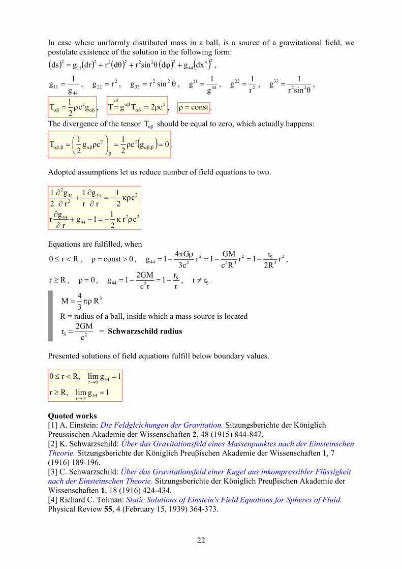
5 BLACK HOLE WITH MAXIMAL ATI-GRAVITY HALO

• Black hole with maximal anti-gravity halo Black hole with maximal anti-gravity halo we will call homogeneous ball with mass (M)

and radius (R), for which

m

kg101.3466

G

c

R

M 272

×≈= .

Spatial radius of a black hole with maximal anti-gravity halo is equal to half of Schwarzschild

radius. Area of outside black hole with maximal anti-gravity halo consist of two layers, in

first ( SS rr r5.0 <≤ ) anti-gravity occures and in second ( Srr > ) – gravity. Thickness of this

anti-gravity shell is equal to spatial radius of black hole with maximal anti-gravity halo.

Inside of anti-gravity layer acceleration is directed from the center of mass source, and inside

of gravity layer – towards the center

Inside of anti-gravity layer acceleration is directed from

the center of a mass source and it grows to the border

with gravity layer. Then acceleration changes direction,

and its absolute value decreases together with a growth

of distance from the center.

This model can be called layer model: anti-gravity –

gravity.

First time model of black hole with maximal anti-gravity halo was proposed by me in 2005 on

the V Forum of Unconventional Inventions, Constructions and Ideas in Wrocław on the

occasion of the 100th anniversary of Einstein's formulation of special theory of relativity. This

Forum was organized by Janusz Zagórski.

27

6 GRAVITATIOAL FIELD ISIDE MASS SOURCE

• Spacetime metric inside mass source

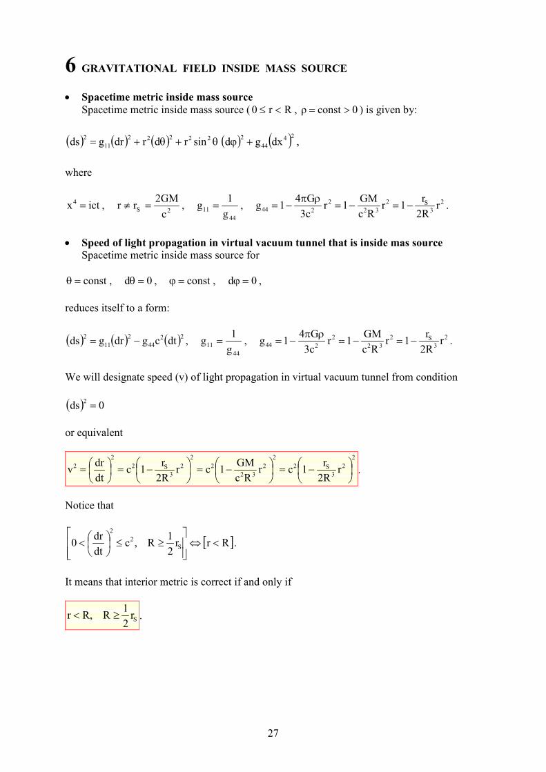
Spacetime metric inside mass source ( Rr0 <≤ , 0constρ >= ) is given by:

( ) ( ) ( ) ( ) ( )24

44

222222

11

2dxgd sinrdrdrgds +ϕθ+θ+= ,

where

ictx4 = , 2S

c

GM2rr =≠ ,

44

11g

1g = , 2

3

S2

32

2

244 r2R

r1r

Rc

GM1r

3c

G41g −=−=

ρπ−= .

• Speed of light propagation in virtual vacuum tunnel that is inside mas source Spacetime metric inside mass source for

const=θ , 0d =θ , const=ϕ , 0d =ϕ ,

reduces itself to a form:

( ) ( ) ( )22

44

2

11

2dtcgdrgds −= ,

44

11g

1g = , 2

3

S2

32

2

244 r2R

r1r

Rc

GM1r

3c

G41g −=−=

ρπ−= .

We will designate speed (v) of light propagation in virtual vacuum tunnel from condition

( ) 0ds2 =

or equivalent

2

2

3

S2

2

2

32

2

2

2

3

S2

2

2 r2R

r1cr

Rc

GM1cr

2R

r1c

dt

drv

−=

−=

−=

= .

Notice that

[ ]Rrr2

1R ,c

dt

dr0 S

2

2

<⇔

≥≤

< .

It means that interior metric is correct if and only if

Sr2

1R R,r ≥< .

28

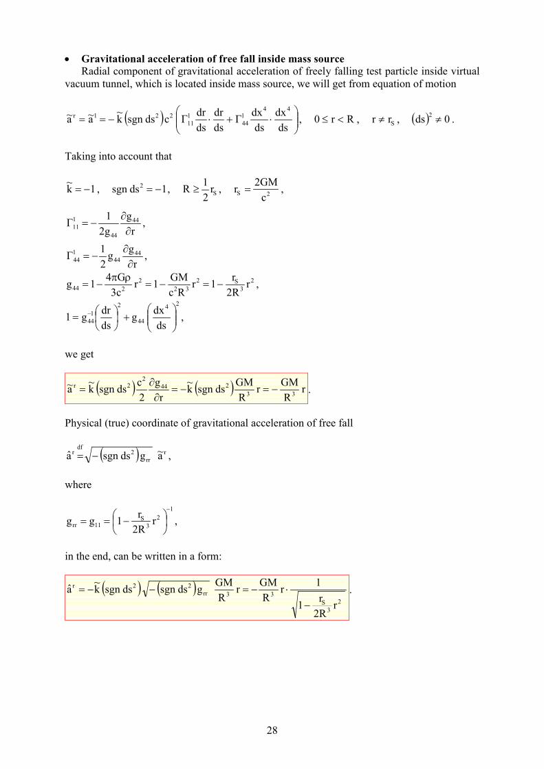
• Gravitational acceleration of free fall inside mass source Radial component of gravitational acceleration of freely falling test particle inside virtual

vacuum tunnel, which is located inside mass source, we will get from equation of motion

( )

⋅+⋅−==

ds

dx

ds

dxΓ

ds

dr

ds

drΓ c ds sgn k

~ a~a~

441

44

1

11

221r , Rr0 <≤ , Srr ≠ , ( ) 0ds2 ≠ .

Taking into account that

1k~

−= , 1dssgn 2 −= , Sr2

1R ≥ ,

2Sc

2GMr = ,

r

g

2g

1Γ 44

44

1

11 ∂∂

−= ,

r

gg

2

1Γ 44

44

1

44 ∂∂

−= ,

2

3

S2

32

2

244 r2R

r1r

Rc

GM1r

3c

G41g −=−=

ρπ−= ,

24

44

2

1

44ds

dx g

ds

drg1

+

= − ,

we get

( ) ( ) r R

GM r

R

GM dssgn k

~

r

g

2

c dssgn k

~a~

33

244

22r −=−=

∂∂

= .

Physical (true) coordinate of gravitational acceleration of free fall

( ) r

rr

2df

r a~ g dssgn a −= ,

where

1

2

3

S11rr r

2R

r1gg

−

−== ,

in the end, can be written in a form:

( ) ( ) r

2R

r1

1r

R

GMr

R

GM g dssgn dssgn k

~a

2

3

S

33rr

22r

−

⋅−=−−= .

29

7 GRAVITATIOAL FIELD ISIDE BLACK HOLE WITH MAXIMAL ATI-

GRAVITY HALO

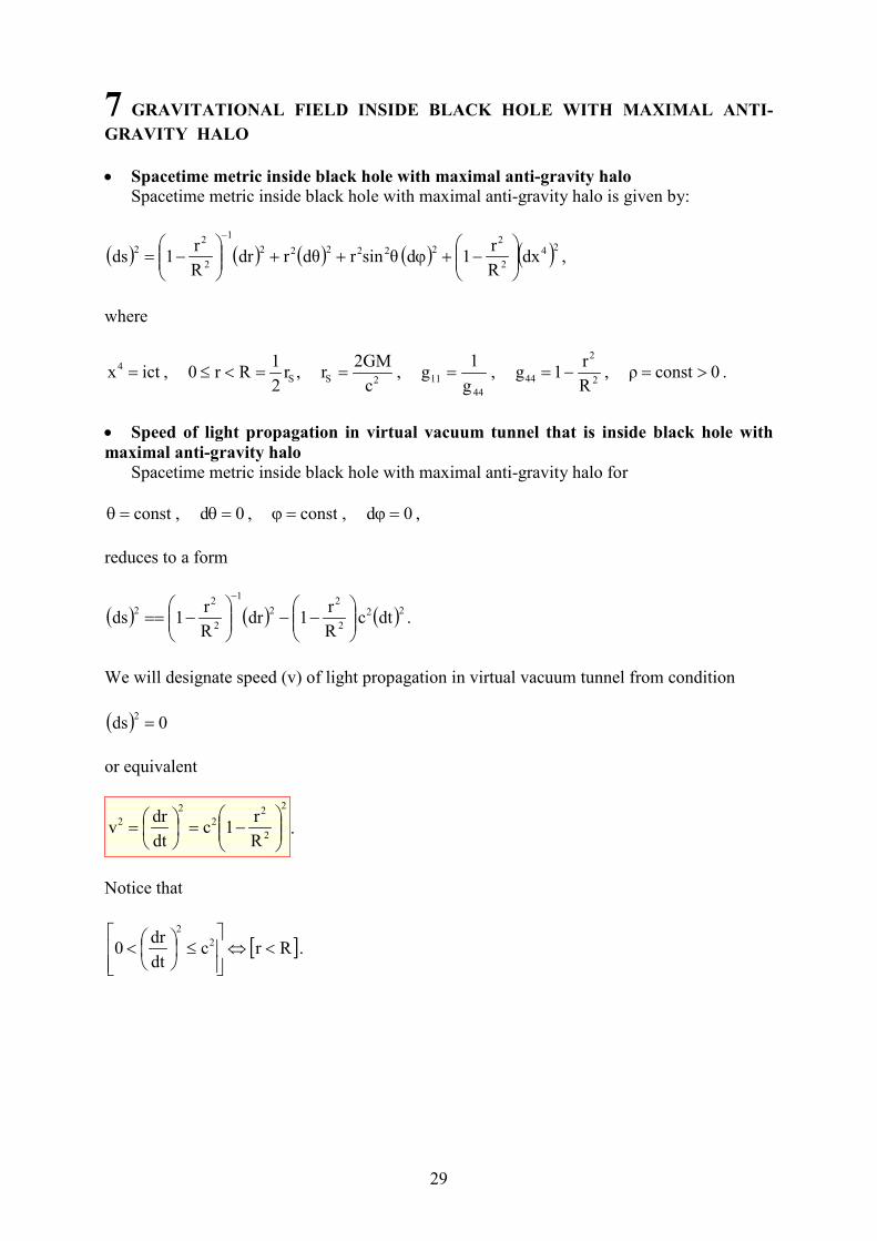
• Spacetime metric inside black hole with maximal anti-gravity halo Spacetime metric inside black hole with maximal anti-gravity halo is given by:

( ) ( ) ( ) ( ) ( )24

2

2222222

1

2

22

dxR

r1d θsinrdθrdr

R

r1ds

−+ϕ++

−=

−

,

where

ictx4 = , Sr2

1Rr0 =<≤ ,

2Sc

GM2r = ,

44

11g

1g = ,

2

2

44R

r1g −= , 0constρ >= .

• Speed of light propagation in virtual vacuum tunnel that is inside black hole with

maximal anti-gravity halo Spacetime metric inside black hole with maximal anti-gravity halo for

const=θ , 0d =θ , const=ϕ , 0d =ϕ ,

reduces to a form

( ) ( ) ( )22

2

22

1

2

22

dtc R

r1dr

R

r1ds

−−

−==

−

.

We will designate speed (v) of light propagation in virtual vacuum tunnel from condition

( ) 0ds2 =

or equivalent

2

2

22

2

2

R

r1c

dt

drv

−=

= .

Notice that

[ ]Rrcdt

dr0 2

2

<⇔

≤

< .

30

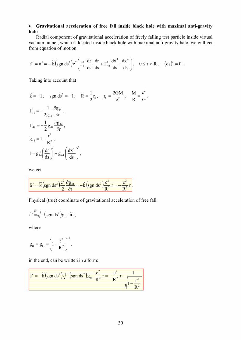
• Gravitational acceleration of free fall inside black hole with maximal anti-gravity

halo Radial component of gravitational acceleration of freely falling test particle inside virtual

vacuum tunnel, which is located inside black hole with maximal anti-gravity halo, we will get

from equation of motion

( )

⋅+⋅−==

ds

dx

ds

dxΓ

ds

dr

ds

drΓ c ds sgn k

~ a~a~

441

44

1

11

221r , Rr0 <≤ , ( ) 0ds2 ≠ .

Taking into account that

1k~

−= , 1dssgn 2 −= , Sr2

1R = ,

2Sc

2GMr = ,

G

c

R

M2

= ,

r

g

2g

1Γ 44

44

1

11 ∂∂

−= ,

r

gg

2

1Γ 44

44

1

44 ∂∂

−= ,

2

2

44R

r1g −= ,

24

44

2

1

44ds

dx g

ds

drg1

+

= − ,

we get

( ) ( ) r R

c r

R

c dssgn k

~

r

g

2

c dssgn k

~a~

2

2

2

2244

22r −=−=

∂∂

= .

Physical (true) coordinate of gravitational acceleration of free fall

( ) r

rr

2df

r a~ g dssgn a −= ,

where

1

2

2

11rrR

r1gg

−

−== ,

in the end, can be written in a form:

( ) ( )

R

r1

1r

R

cr

R

c g dssgn dssgn k

~a

2

22

2

2

2

rr

22r

−

⋅−=−−= .

31

8 GRAPHIC AALYSIS OF THE FULL SOLUTIO

• Charts that show how time-time component of metric tensor and physical (true)

coordinate of gravitational acceleration of free fall depends on the distance from the

center of black hole with maximal anti-gravity halo We will make those charts for case, where spatial radius of black hole is half of Schwarz-

schild radius

2Sc

GMr

2

1R == ,

which is for black hole with maximal anti-gravity halo.

Time-time component of metric tensor and physical (true) coordinate of gravitational

acceleration of free fall, in three distance intervals from the center of blach hole, are given by

below relations.

GRAVITY

Sr2

1r0 <≤ , 0

R

r1g

2

2

44 >

−= ,

R

r1

1r

R

ca

2

22

2r

−

⋅−=

ATI-GRAVITY

SS rrr 2

1<≤ , 0

r

r1g S

44 <

−= ,

1r

r

1

r

GM a

S

2

r

−

⋅+=

GRAVITY

Srr > , 0r

r1g S

44 >

−= ,

r

r1

1

r

GM a

S

2

r

−

⋅−=

1

0r

g44

R = 0.5rS

rS

1

Chart that shows how time-time component of metric tensor depends on the distance from the

center of black hole with maximal anti-gravity halo.

32

1

0r

g44

R = 0.5rS

rS

1

Chart that shows how time-time component of metric tensor depends on the distance from the

center of bkack hole with maximal anti-gravity halo.

ra

2r

GM

0r

ra

2r

GM

R = 0.5rS

rS

Chart of dependence of radial coordinate of physical (true) gravitational acceleration of free

fall on the distance from the center of black hole with maximal anti-gravity halo.

ATTETIOFirst graph is doublet for better clearness on the same page.

From the charts we can see that:

Sr 5.0r0 ⋅<≤ ⇒ gravity

Sr 5.0r ⋅= ⇒ transition from gravity to anti-gravity

SS r rr 5.0 <<⋅ ⇒ anti-gravity

Sr r = ⇒ transition from anti-gravity to gravity

Sr r > ⇒ gravity

Gravity and anti-gravity has layer-like nature.

33

9 FIELD EQUATIOS AD EQUATIOS OF MOTIO

• Equations of motion are contained in field equations How schould one formulate equations of motion, so that non-rescaled radial coordinates

of 4-acceleration could be served with below forms?

( ) ( ) ( ) 0 dssgn 1,k~

R,r0 r, R

GM dssgn k

~r

R

GM

ds

rdc dssgn a~ 2

3

2

32

222

dfr

in <−=<≤−=−==

( ) ( ) ( ) 0dssgn 1,k~

R,r ,r

GM dssgn k

~

r

GM

ds

rdc dssgn a~ 2

2

2

22

222

dfr

ex <+=>=−==

While answering to this question, we will use second of two field equations.

( )1g2r

crG2

r

g

2

c

G4c

2

r

g

r

2

r

g

in

44

2in

44

2

2

in

44

2

in

44

2

−−ρπ−=∂

∂

ρπ⋅−=∂

∂+

∂∂

2

3

S2

32

2

2

in

44 r2R

r1r

Rc

GM1r

3c

G41g −=−=

ρπ−=

rR

GMρrG

3

4

r

g

2

c3

in

44

2

−=π−=∂

∂

( ) ( ) r R

GM dssgn k

~r

R

GM

ds

rdc dssgn a~

3

2

32

222

dfr

in −=−==

( )r

g

2

c dssgn k

~a~

in

44

22r

in ∂∂

=

r

g

2

1

ds

dx

ds

dxΓ

ds

dr

ds

drΓ

in

44

441

44

1

11 ∂∂

−=⋅+⋅

( )

⋅+⋅−=

ds

dx

ds

dxΓ

ds

dr

ds

drΓc dssgn k

~a~

441

44

1

11

22r

in

Analogical consideration for coordinate r

exa~ leads to a conclusion, that equations of motion

should have the form served below:

( ) ( )ds

dx

ds

dx c dssgn k

~

ds

xdc dssgn a~ 22

2

222

df νµαµν

αα ⋅Γ−==

source mass a of inside 1

source mass a of outside 1

−

+=k

~

34

• Equations of motion and field equations in General Relativity, and 2-potential nature

of ewton’s stationary gravitational field Postulated by us, within the frames of General Relativity, equations of motion of free test

particle, leads to a conclusion, that Newton’s stationary gravitational field is a 2-potential

field. We will show it on an example of gravitational field, which source is a mass distributed

homogeneously in a volume of a ball with radius R.

( ) ( ) 0g dssgn ,0dxdxgds ,ds

dx

ds

dx c dssgn k

~ a~

m

F~

2222 ≤≠=Γ+= µννµ

µν

νµαµν

αα

0F~

=α

rx1 = , θ=2x , ϕ=3x , ictx 4 =

( ) ( ) ( ) ( ) ( )24

44

222222

11

2dxgd θsinrdθrdrgds +ϕ++=

44

11g

1g = , 2

22 rg = , θ= 22

33 sinrg

r

g

2

1

ds

dx

ds

dxΓ

ds

dr

ds

drΓ 44

441

44

1

11 ∂∂

−=⋅+⋅

( )r

g

2

c dssgn k

~a~ 44

22r

∂∂

=

r

ina , r

exa = radial acceleration respectively inside and outside of a ball

in

44g , ex

44g = metric tensor components respectively inside and outside of a ball

2

3

S2

32

2

2

in

44 r2R

r1r

Rc

GM1r

3c

G41g −=−=

ρπ−= , Rr0 <≤ , 0constρ >=

r

r1

rc

2GM1g S

2

ex

44 −=−= , Rr ≥ , Rr ≥ , 0ρ =

( ) ( ) Rr0 r, R

GMdssgn k

~

r

g

2

c dssgn k

~a~

3

2in

44

22r

in <≤−=∂

∂=

( ) ( ) Rr ,r

GM dssgn k

~

r

g

2

c dssgn k

~a~

2

2ex

44

22r

ex ≥=∂

∂=

Srr >> , 22 cv << , 2S

c

2GMr =

2

2r

dt

rd a = , 1dssgn 2 −= ,

ball shomogeneou of nsidei 1

ball shomogeneou of utside 1k~

−

+=

o

Rr0 r, R

GM

r

g

2

c k

~a

3

in

44

2r

in <≤−=∂

∂−=

Rr ,r

GM

r

g

2

c k

~a

2

ex

44

2r

ex ≥−=∂

∂−=

35

By substitution in last two equations

2

in

in

44c

21g

ϕ+= ,

2

ex

ex

44c

21g

ϕ+= ,

where ( inϕ ) and ( exϕ ) are potentials of gravitational field respectively inside and outside of a

ball, we will get

Now lets serve definition of potentials ( inϕ ) and ( exϕ ) that corresponds with standard defini-

tion of gravitational potential.

r

GMdr a

r2R

GMdr a

Rr

r

ex

dfex

2

3

Rr

0

r

in

dfin

−=−=ϕ

−==ϕ

∫

∫∞

≥

<

We will serve field equations inside mass source, in a form convienient for further con-

templation.

( ) ρG4c

21g

r

2

r

g

r

2

ρG4c

2

r

g

r

2

r

g

2

in

442

in

44

2

in

44

2

in

44

2

π⋅−=−+∂

∂

π⋅−=∂

∂+

∂∂

2

in

in

44c

21g

ϕ+=

ρG4r

2

r r

2

ρG4r r

2

r

in

2

in

in

2

in2

π−=ϕ+∂

ϕ∂

π−=∂

ϕ∂+

∂

ϕ∂

First of those equations is a Poisson’s equation for potential ( inϕ ) in spherical coordinate

system. From classical Poisson’s equation it differs only in sign of right side. Then, from both

equations it appears that

in

22

in2

r

2

r ϕ=

∂

ϕ∂

rR

GM

rr k

~a

3

inin

r

in −=∂

ϕ∂=

∂

ϕ∂−= , Rr0 <≤ , 2

3

in r2R

GM−=ϕ , 0 lim in

0r=ϕ

→

2

exex

r

exr

GM

r

r k

~a −=

∂

ϕ∂−=

∂

ϕ∂−= , Rr ≥ ,

r

GMex −=ϕ , 0 lim ex

r=ϕ

∞→

Poisson’s equation for potential inϕ

36

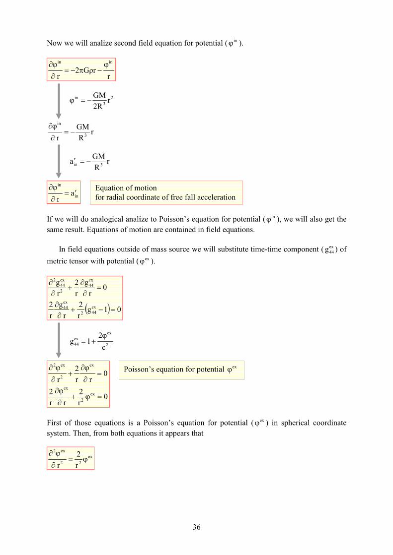
Now we will analize second field equation for potential ( inϕ ).

rρrG2

r

inin ϕ−π−=

∂

ϕ∂

2

3

in r2R

GM−=ϕ

rR

MG

r 3

in

−=∂

ϕ∂

rR

GMa

3

r

in −=

r

in

in

ar

=∂

ϕ∂

If we will do analogical analize to Poisson’s equation for potential ( inϕ ), we will also get the

same result. Equations of motion are contained in field equations.

In field equations outside of mass source we will substitute time-time component ( ex

44g ) of

metric tensor with potential ( exϕ ).

( ) 01gr

2

r

g

r

2

0r

g

r

2

r

g

ex

442

ex

44

ex

44

2

ex

44

2

=−+∂

∂

=∂

∂+

∂∂

2

ex

ex

44c

21g

ϕ+=

0r

2

r r

2

0r r

2

r

ex

2

ex

ex

2

ex2

=ϕ+∂

ϕ∂

=∂

ϕ∂+

∂

ϕ∂

First of those equations is a Poisson’s equation for potential ( exϕ ) in spherical coordinate

system. Then, from both equations it appears that

ex

22

ex2

r

2

r ϕ=

∂

ϕ∂

Equation of motion

for radial coordinate of free fall acceleration

Poisson’s equation for potential exϕ

37

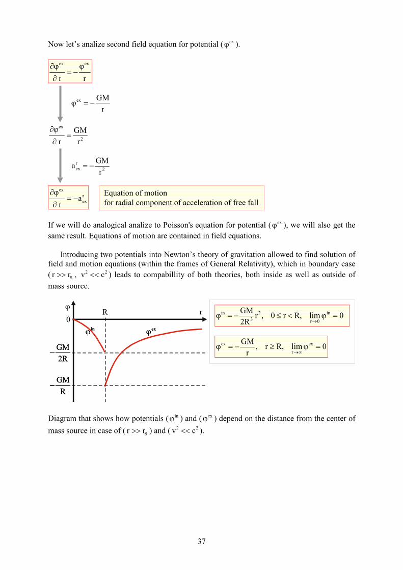
Now let’s analize second field equation for potential ( exϕ ).

rr

exex ϕ−=

∂

ϕ∂

r

GMex −=ϕ

2

ex

r

GM

r =

∂

ϕ∂

2

r

exr

GMa −=

r

ex

ex

ar

−=∂

ϕ∂

If we will do analogical analize to Poisson's equation for potential ( exϕ ), we will also get the

same result. Equations of motion are contained in field equations.

Introducing two potentials into Newton’s theory of gravitation allowed to find solution of

field and motion equations (within the frames of General Relativity), which in boundary case

( Srr >> , 22 cv << ) leads to compabillity of both theories, both inside as well as outside of

mass source.

2R

GM−

R

GM−

inϕ exϕ

rR0

ϕ

2R

GM−

R

GM−

inϕ exϕ

Diagram that shows how potentials ( inϕ ) and ( exϕ ) depend on the distance from the center of

mass source in case of ( Srr >> ) and ( 22 cv << ).

Equation of motion

for radial component of acceleration of free fall

0 lim R,r0,r2R

GM in

0r

2

3

in =ϕ<≤−=ϕ→

0 lim R,r ,r

GM ex

r

ex =ϕ≥−=ϕ∞→

38

2R

GM−

R

GM−

inϕ exϕ

rR0

ϕ

2R

GM−

R

GM−

inϕ exϕ

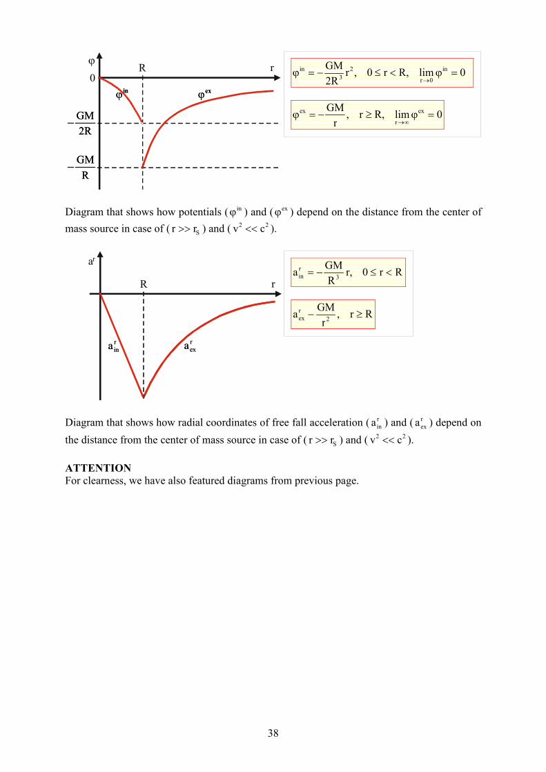
Diagram that shows how potentials ( inϕ ) and ( exϕ ) depend on the distance from the center of

mass source in case of ( Srr >> ) and ( 22 cv << ).

r

inar

exa

rR

r

inar

exa

ar

Diagram that shows how radial coordinates of free fall acceleration ( r

ina ) and ( r

exa ) depend on

the distance from the center of mass source in case of ( Srr >> ) and ( 22 cv << ).

ATTETIOFor clearness, we have also featured diagrams from previous page.

Rr0 r, R

GMa

3

r

in <≤−=

Rr ,r

GM a

2

r

ex ≥−

0 lim R,r0,r2R

GM in

0r

2

3

in =ϕ<≤−=ϕ→

0 lim R,r ,r

GM ex

r

ex =ϕ≥−=ϕ∞→

39

10 EW TEST OF GEERAL RELATIVITY

• The proposition of the experiment How to show in Earth conditions, 2-potential nature of gravitational field and also prove

the existence of black holes with anti-gravity halo? In this purpose we have to measure ratio

of distance passed by light to the time of flight, in a vertically positioned vacuum cylinder,

right under and right above the surface of Earth (of the sea level). If the difference of squares

of those measurements will be equal to the square of escape speed, then it will prove exis-

tence of black holes with anti-gravity halo. This experiment would be a new test of General

Theory of Relativity.

Below we will justify purpose of this experiment:

?dt

dr

dt

dr2

ex

2

in

=

−

indt

dr

i

exdt

dr

– ratio of path travelled by the light to the time of travel

measured respectively right under and right over Eartt surface

2

2

3

S2

2

in

r2R

r1c

dt

dr

−=

2

S2

2

ex r

r1c

dt

dr

−=

Rr ≈

2S

c

GM2r =

1R

rS <<

c2dt

dr

dt

dr

exin

≈

+

2

s

km91.7

R

GM

=

s

m103

s

m102.99792458c 88 ⋅≈⋅=

R

2GM

dt

dr

dt

dr2

ex

2

in

≅

−

s

m0.208

cR

GM

dt

dr

dt

dr

exin

≅≅

−

40

rS

0.5rS

0.5rS

GRAVITY

ANTI-GRAVITY

GRAVITY

11 BLACK HOLE MODEL OF OUR UIVERSE

• Our Universe as a black hole with maximal anti-gravity halo

In the center of black hole, gravitational acceleration of

free particle is equal to zero which corresponds with

Gauss law. Later, absolute value of acceleration grows

together with growth of distance from the center. In

anti-gravity layer, gravitational acceleration is pointed

from the center of mass source and it grows to the

gravity-layer bordeline. Then, acceleration turns direc-

tion, and its absolute value decreases with growth of

distance from the center.

This model can be called „layer model

gravity-anti-gravity-gravity

Our Universe can be treated as a gigantic, homogeneous Black Hole. It is isolated from the

rest of universe with a space area where anti-gravity occures. Our galaxy together with Solar

system and Earth (which in cosmological scales can be treated merely as a point) should be

located near the center of Black Hole. Once again let’s remind that in the center of black hole,

gravitational acceleration of free particle, leaving out local gravitational fields, is equal to ze-

ro. In other words: Black Hole is not generating gravitational field in its center.

• Radius of Our Universe Below, let’s estimate radius of Our Universe, assuming that, its average density is the

same as density (np) of protons in every cubic meter.

2Sc

GMr

2

1R ==

3πρR3

4M =

ρ

1

G4

3cR

2

⋅π

=

s

m103

s

m10 2.99792458c 88 ⋅≈⋅= ,

2

311

2

311

skg

m106.7

skg

m106.6742G

⋅⋅≈

⋅⋅= −−

3

27

pm

kg101.67n −⋅⋅≈ρ

pn = average amount of protons in every cubic meter

kg1067262171.1m 27

p

−⋅= = proton mass

light year m100.95 16⋅≈

yearslight 10 n

19.501m10

n

19R 9

p

26

p

⋅⋅≈⋅≈

41

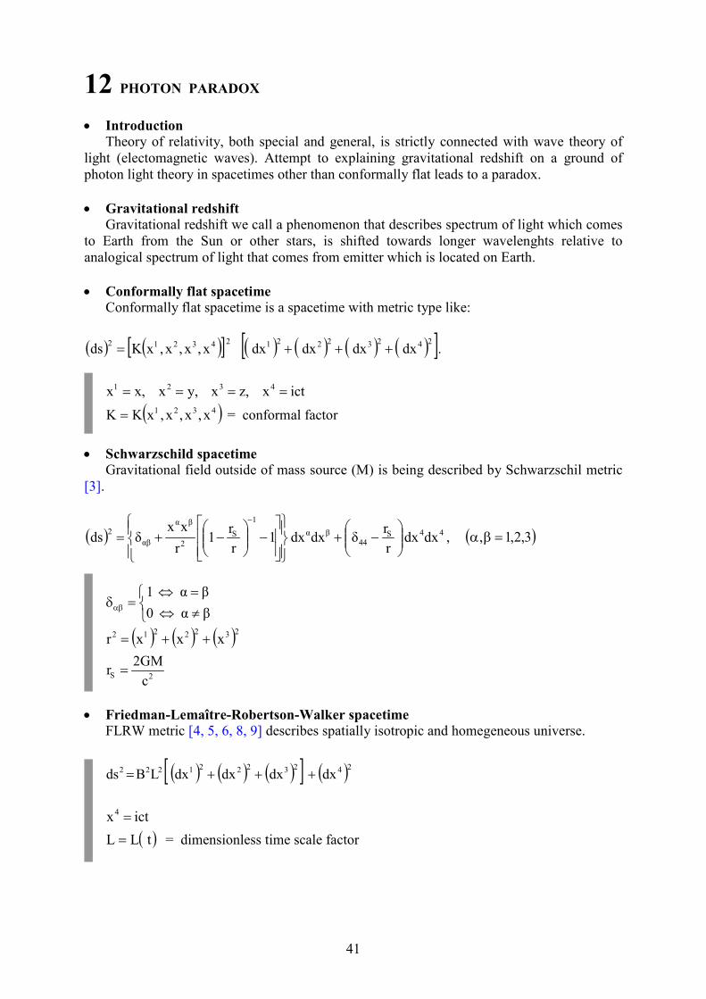
12 PHOTO PARADOX

• Introduction Theory of relativity, both special and general, is strictly connected with wave theory of

light (electomagnetic waves). Attempt to explaining gravitational redshift on a ground of

photon light theory in spacetimes other than conformally flat leads to a paradox.

• Gravitational redshift Gravitational redshift we call a phenomenon that describes spectrum of light which comes

to Earth from the Sun or other stars, is shifted towards longer wavelenghts relative to

analogical spectrum of light that comes from emitter which is located on Earth.

• Conformally flat spacetime Conformally flat spacetime is a spacetime with metric type like:

( ) ( )[ ] ( ) ( ) ( ) ( )[ ]242322212 43212dx dx dx dx x,x,x,xKds +++= .

ict xz, xy, xx,x 4321 ====

( ) x,x,x,xKK 4321= = conformal factor

• Schwarzschild spacetime Gravitational field outside of mass source (M) is being described by Schwarzschil metric

[3].

( ) 44S44

βα

1

S

2

βα

αβ

2dxdx

r

rδdxdx 1

r

r1

r

xxδds

−+

−

−+=

−

, ( )3,2,1, =βα

≠⇔

=⇔=δαβ

βα 0

βα 1

( ) ( ) ( )2322212 xxxr ++=

2Sc

GM2r =

• Friedman-Lemaître-Robertson-Walker spacetime FLRW metric [4, 5, 6, 8, 9] describes spatially isotropic and homegeneous universe.

( ) ( ) ( )[ ] ( )24232221222 dx dxdxdx LBds +++=

ictx4 =

( )t LL = = dimensionless time scale factor

42

2

41

2

2

41

22

22

41

kr1

1

a

r1

1

aL

rL1

1B

+=

+=

+=

( ) ( ) ( )2322212 xxxr ++=

2a

1k = , 1 ,0 ,1

a

1sgn ksgn

2+−==

2a = square of non-rescaled constant radius of space curavutre

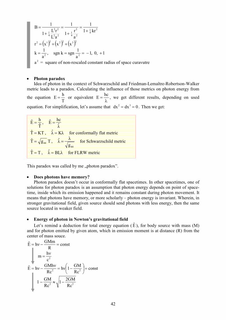
• Photon paradox Idea of photon in the context of Schwarzschild and Friedman-Lemaître-Robertson-Walker

metric leads to a paradox. Calculating the influence of those metrics on photon energy from

the equation T

hE = or equivalent

λ=

hcE , we get different results, depending on used

equation. For simplification, let’s assume that . 0dxdx 32 == Then we get:

This paradox was called by me „photon paradox”.

• Does photons have memory? Photon paradox doesn’t occur in conformally flat spacetimes. In other spacetimes, one of

solutions for photon paradox is an assumption that photon energy depends on point of space-

time, inside which its emission happened and it remains constant during photon movement. It

means that photons have memory, or more scholarly – photon energy is invariant. Wherein, in

stronger gravitational field, given source should send photons with less energy, then the same

source located in weaker field.

• Energy of photon in ewton’s gravitational field

Let’s remind a deduction for total energy equation ( E ), for body source with mass (M)

and for photon emitted by given atom, which in emission moment is at distance (R) from the

center of mass souce.

constR

GMmhνE =−=

2c

hm

ν=

constRc

GM1hν

Rc

GMhνhνE

22=

−=−=

22 cR

GM21

cR

GM−≈−1

T

hE = ,

λ

hcE =

KTT = , Kλλ = for conformally flat metric

T gT 44= , 44g

λλ = for Schwarzschild metric

TT = , BLλλ = for FLRW metric

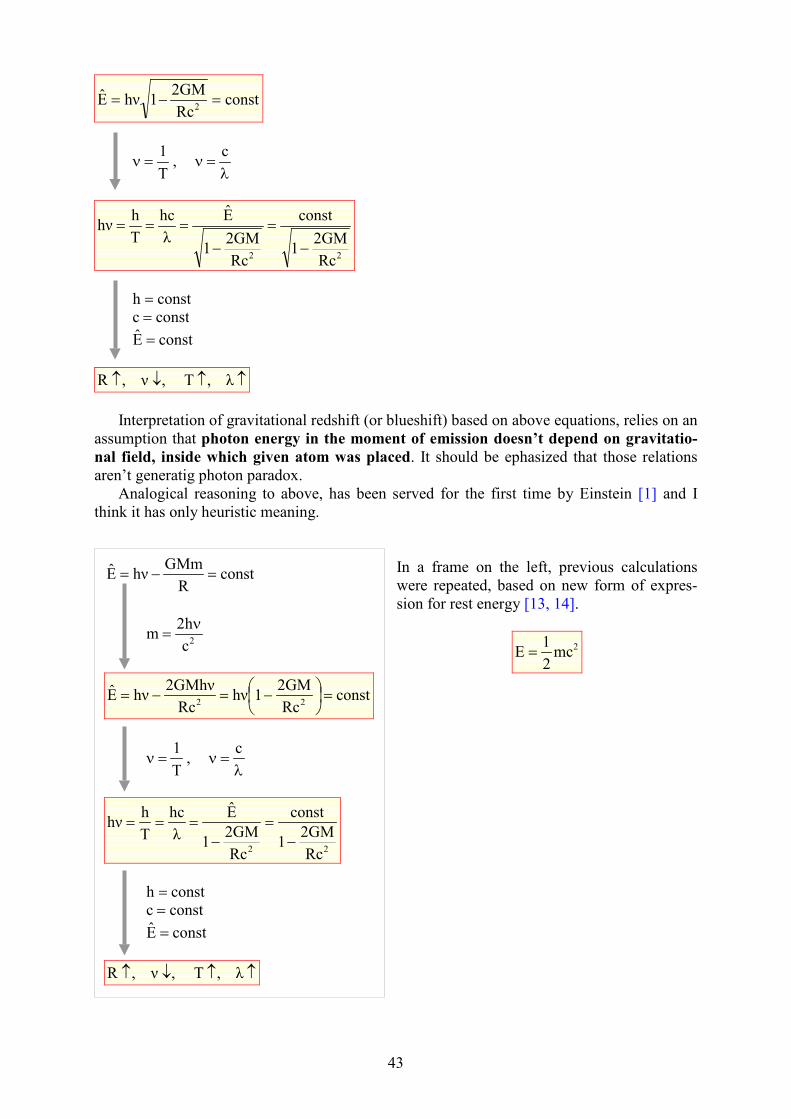
43

constRc

2GM1hνE

2=−=

T

1=ν ,

λ=ν

c

22 Rc

2GM1

const

Rc

2GM1

E

λ

hc

T

hhν

−

=

−

===

consth = constc = constE =

↑↑↓↑ λ ,T ,ν ,R

Interpretation of gravitational redshift (or blueshift) based on above equations, relies on an

assumption that photon energy in the moment of emission doesn’t depend on gravitatio-

nal field, inside which given atom was placed. It should be ephasized that those relations

aren’t generatig photon paradox.

Analogical reasoning to above, has been served for the first time by Einstein [1] and I

think it has only heuristic meaning.

In a frame on the left, previous calculations

were repeated, based on new form of expres-

sion for rest energy [13, 14].

2mc2

1E =

constR

GMmhνE =−=

2c

h2m

ν=

constRc

2GM1hν

Rc

2GMhνhνE

22=

−=−=

T

1=ν ,

λ=ν

c

22 Rc

2GM1

const

Rc

2GM1

E

λ

hc

T

hhν

−=

−===

consth = constc = constE =

↑↑↓↑ λ ,T ,ν ,R

44

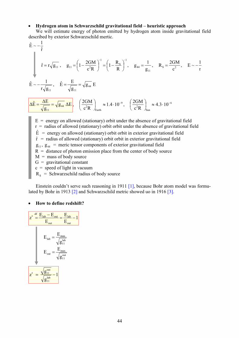
• Hydrogen atom in Schwarzschild gravitational field – heuristic approach We will estimate energy of photon emitted by hydrogen atom inside gravitational field

described by exterior Schwarzschild mertic.

r

1~E −

11grr = ,

1

S

1

211R

R1

Rc

2GM1g

−−

−=

−= , 11

44g

1g = ,

2Sc

GM2R = ,

r

1~E −

11gr

1~E − , E g

g

E E 44

11

==

∆E gg

∆EE∆ 44

11

== , 9

Earth

2101.4

Rc

2GM −⋅≈

, 6

2104.3

Rc

2GM −⋅≈

Sun

E = energy on allowed (stationary) orbit under the absence of gravitational field

r = radius of allowed (stationary) orbit orbit under the absence of gravitational field

E = energy on allowed (stationary) orbit orbit in exterior gravitational field

r = radius of allowed (stationary) orbit orbit in exterior gravitational field

11g , 44g = meric tensor components of exterior gravitational field

R = distance of photon emission place from the center of body source

M = mass of body source

G = gravitational constant

c = speed of light in vacuum

SR = Schwarzschild radius of body source

Einstein couldn’t serve such reasoning in 1911 [1], because Bohr atom model was formu-

lated by Bohr in 1913 [2] and Schwarzschild metric showed uo in 1916 [3].

• How to define redshift?

1E

E

E

EE z

out

lab

out

outlabdf

−=−

=∗

lab

11

maxlab

g

EE =

out

11

maxout

g

EE =

1g

g z

lab

11

out

11 −=∗

45

labE = photon energy emitted from a source that is in laboratory

outE = photon energy emitted from a source that is outside laboratory

maxE = photon energy emitted from a source in the absence of gravitational field

lab

11g = component of metric tensor in laboratory in a place of photon detectionout

11g = component of metric tensor outside of laboratory in a place of photon emission

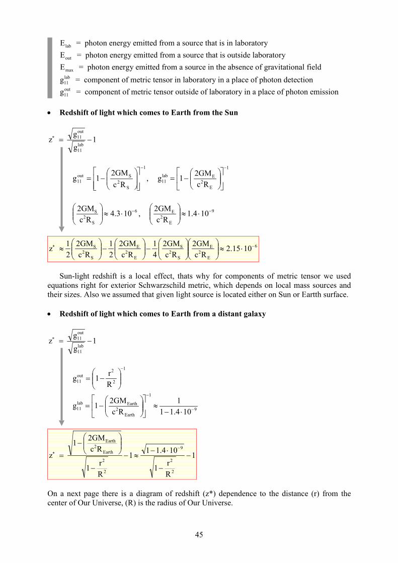
• Redshift of light which comes to Earth from the Sun

1g

g z

lab

11

out

11 −=∗

1

S

2

Sout

11Rc

2GM1g

−

−= ,

1

E

2

Elab

11Rc

2GM1g

−

−=

6

S

2

S 104.3Rc

2GM −⋅≈

, 9

E

2

E 101.4Rc

2GM −⋅≈

6

E

2

E

S

2

S

E

2

E

S

2

S 1015.2Rc

2GM

Rc

2GM

4

1

Rc

2GM

2

1

Rc

2GM

2

1 z −∗ ⋅≈

−

−

≈

Sun-light redshift is a local effect, thats why for components of metric tensor we used

equations right for exterior Schwarzschild metric, which depends on local mass sources and

their sizes. Also we assumed that given light source is located either on Sun or Eartth surface.

• Redshift of light which comes to Earth from a distant galaxy

1g

g z

lab

11

out

11 −=∗

1

2

2out

11R

r1g

−

−=

9

1

Earth

2

Earthlab

11104.11

1

Rc

2GM1g −

−

⋅−≈

−=

1

R

r1

104.111

R

r1

Rc

2GM1

z

2

2

9

2

2

Earth

2

Earth

−

−

⋅−≈−

−

−

=−

∗

On a next page there is a diagram of redshift (z*) dependence to the distance (r) from the

center of Our Universe, (R) is the radius of Our Universe.

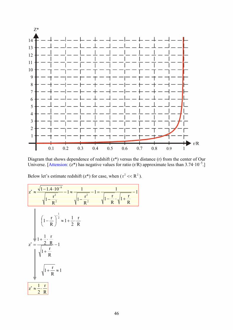
46

0.1 0.2 0.3 0.4 0.5 0.6 0.7 0.8 0.9 1

1

2

3

4

5

6

7

8

9

10

11

12

13

14

Z*

r/R

Diagram that shows dependence of redshift (z*) versus the distance (r) from the center of Our

Universe. [Attension: (z*) has negative values for ratio (r/R) approximate less than 3.74·10–5

.]

Below let’s estimate redshift (z*) for case, when ( 22 Rr << ).

1

R

r1

R

r1

11

R

r1

11

R

r1

104.11 z

2

2

2

2

9

−

+⋅−

=−

−

≈−

−

⋅−≈

−∗

R

r

2

11

R

r1

2

1

⋅+≈

−

−

1

R

r1

R

r

2

11

z −

+

⋅+=∗

1R

r1 ≈+

R

r

2

1 z ⋅≈∗

47

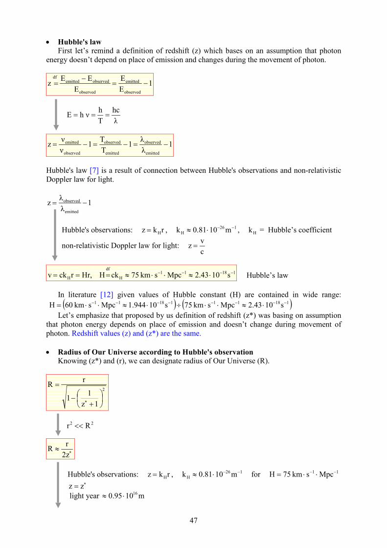
• Hubble's law First let’s remind a definition of redshift (z) which bases on an assumption that photon

energy doesn’t depend on place of emission and changes during the movement of photon.

1E

E

E

EE z

observed

emitted

observed

observedemitteddf

−=−

=

λ

hc

T

hνh E ===

1λ

λ1

T

T1

ν

ν z

emitted

observed

emitted

observed

observed

emitted −=−=−=

Hubble's law [7] is a result of connection between Hubble's observations and non-relativistic

Doppler law for light.

1λ

λ z

emitted

observed −=

Hubble's observations: rk z H= , 162

H m100.81k −−⋅≈ , Hk = Hubble’s coefficient

non-relativistic Doppler law for light: c

v z =

11811

H

df

H s102.43Mpcskm 75ckH Hr,rck v −−−− ⋅≈⋅⋅≈=== Hubble’s law

In literature [12] given values of Hubble constant (H) are contained in wide range:

( ) ( )1181111811 s102.43Mpcskm 57s101.944Mpcskm 06H −−−−−−−− ⋅≈⋅⋅÷⋅≈⋅⋅= Let’s emphasize that proposed by us definition of redshift (z*) was basing on assumption

that photon energy depends on place of emission and doesn’t change during movement of

photon. Redshift values (z) and (z*) are the same.

• Radius of Our Universe according to Hubble's observation Knowing (z*) and (r), we can designate radius of Our Universe (R).

2

1z

11

rR

+

−

=

∗

22 Rr <<

∗≈2z

rR

Hubble's observations: rk z H= , 162

H m100.81k −−⋅≈ for 11 Mpcskm 57H −− ⋅⋅=

∗= zz

light year m100.95 16⋅≈

48

yearslight billion 6.31m106.02k

1R 26

H

≈⋅≈≈

• Average density of Our Universe according to Hubble's observation Now let’s calculate average density of Our Universe, using estimated above radius value

of Our Universe and equation from page 40.

ρ

1

G4

3cR

2

⋅π

=

G

H3

G

k3c

R

1

G4

3cρ

22

H

2

2

2

π=

π≈⋅

π=

m106.0RR 26

H ⋅≈= = radius of Our Universe for 11 Mpcskm 57H −− ⋅⋅=

Hρ=ρ = density of Our Universe for 11 Mpcskm 57H −− ⋅⋅=

327

F mkg1097.4ρ −⋅≈ that is almost 3 protons per every cubic meter

Fρ = density of Friedman Universe according to [11] for 11 Mpcskm 57H −− ⋅⋅= and

47.0=Ω

327

H mkg1059.48ρ −− ⋅⋅≈ that is almost 51 protons/m3

02.17ρ

ρ

F

H ≈

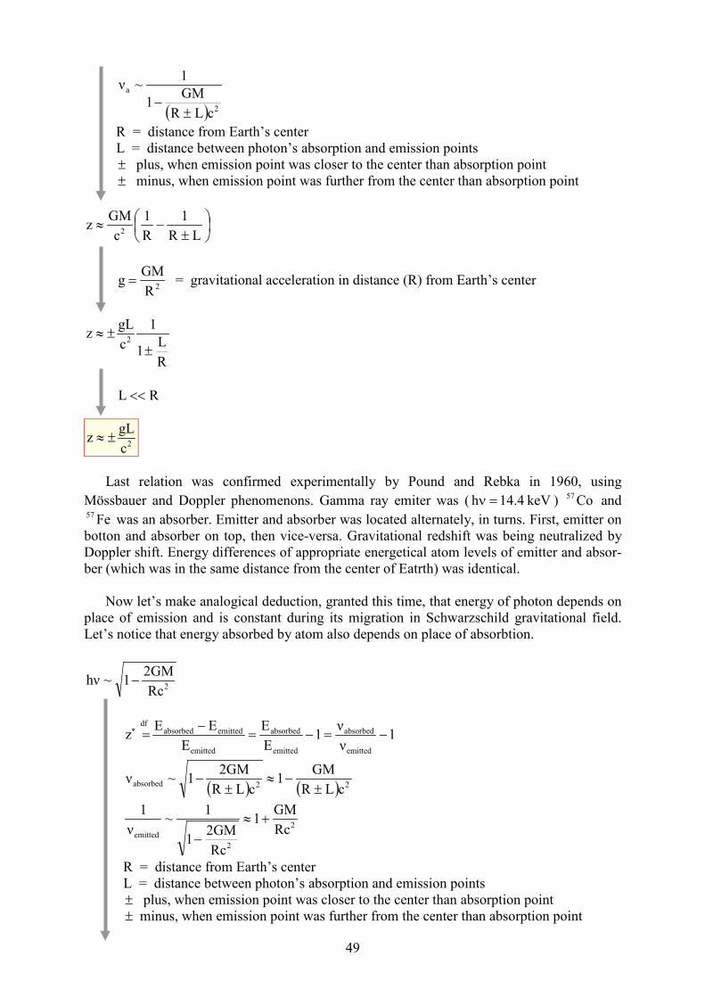
• Constancy of photon energy and Pound-Rebka experiment The purpose of Pound-Rebka experiment [10] was to prove a hypothesis, that photon

energy doesn’t depend on place of emission and changes during movement in Newton’s

gravitational field. Therefore result from this hyphothesis is also: energy absorbed by atom

doesn’t depend on place of absorption.

2Rc

GM1

1~hν

−

1ν

ν z

absorbed

emitteddf

−=

2

2

eRc

GM1

Rc

GM1

1~ν +≈

−

For Hubble’s constant 11 Mpcskm 57H −− ⋅⋅= and density parameter 47.0=Ω density of

Black Hole Universe is over 17 times bigger than density of Friedman Universe.

Our model doesn’t require us to assume the existence of dark energy.

This density is 8 times bigger than critical density

of Friedman Universe.

49

( ) 2

a

cLR

GM1

1~ν

±−

R = distance from Earth’s center

L = distance between photon’s absorption and emission points

± plus, when emission point was closer to the center than absorption point

± minus, when emission point was further from the center than absorption point

±

−≈LR

1

R

1

c

GMz

2

2R

GMg = = gravitational acceleration in distance (R) from Earth’s center

R

L1

1

c

gLz

2

±±≈

RL <<

2c

gLz ±≈

Last relation was confirmed experimentally by Pound and Rebka in 1960, using

Mössbauer and Doppler phenomenons. Gamma ray emiter was ( keV 14.4h =ν ) Co57 and

Fe57 was an absorber. Emitter and absorber was located alternately, in turns. First, emitter on

botton and absorber on top, then vice-versa. Gravitational redshift was being neutralized by

Doppler shift. Energy differences of appropriate energetical atom levels of emitter and absor-

ber (which was in the same distance from the center of Eatrth) was identical.

Now let’s make analogical deduction, granted this time, that energy of photon depends on

place of emission and is constant during its migration in Schwarzschild gravitational field.

Let’s notice that energy absorbed by atom also depends on place of absorbtion.

2Rc

2GM1~hν −

1ν

ν1

E

E

E

EE z

emitted

absorbed

emitted

absorbed

emitted

emittedabsorbeddf

−=−=−

=∗

( ) ( ) 22absorbed

cLR

GM1

cLR

2GM1~ν

±−≈

±−

2

2

emitted Rc

GM1

Rc

2GM1

1~

ν

1+≈

−

R = distance from Earth’s center

L = distance between photon’s absorption and emission points

± plus, when emission point was closer to the center than absorption point

± minus, when emission point was further from the center than absorption point

50

±

−≈∗

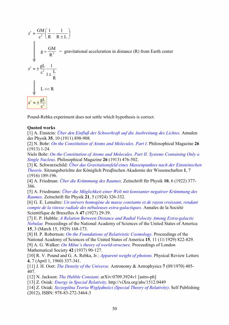
LR

1

R

1

c

GMz

2

2R

GMg = = gravitational acceleration in distance (R) from Earth center

R

L1

1

c

gLz

2

±±≈∗

RL <<

2c

gLz ±≈∗

Pound-Rebka experiment does not settle which hypothesis is correct.

Quoted works[1] A. Einstein: Über den Einfluß der Schwerkraft auf die Ausbreitung des Lichtes. Annalen

der Physik 35, 10 (1911) 898-908.

[2] N. Bohr: On the Constitution of Atoms and Molecules. Part I. Philosophical Magazine 26

(1913) 1-24.

Niels Bohr: On the Constitution of Atoms and Molecules. Part II. Systems Containing Only aSingle 7ucleus. Philosophical Magazine 26 (1913) 476-502.

[3] K. Schwarzschild: Über das Gravitationsfeld eines Massenpunktes nach der EinsteinschenTheorie. Sitzungsberichte der Königlich Preuβischen Akademie der Wissenschaften 1, 7

(1916) 189-196.

[4] A. Friedman: Über die Krümmung des Raumes. Zeitschrift für Physik 10, 6 (1922) 377-

386.

[5] A. Friedmann: Über die Möglichkeit einer Welt mit konstanter negativer Krümmung desRaumes. Zeitschrift für Physik 21, 5 (1924) 326-332.

[6] G. E. Lemaître: Un univers homogène de masse constante et de rayon croissant, rendantcompte de la vitesse radiale des nébuleuses extra-galactiques. Annales de la Société

Scientifique de Bruxelles A 47 (1927) 29-39.

[7] E. P. Hubble: A Relation Between Distance and Radial Velocity Among Extra-galactic7ebulae. Proceedings of the National Academy of Sciences of the United States of America

15, 3 (March 15, 1929) 168-173.

[8] H. P. Robertson: On the Foundations of Relativistic Cosmology. Proceedings of the

National Academy of Sciences of the United States of America 15, 11 (11/1929) 822-829.

[9] A. G. Walker: On Milne’s theory of world-structure. Proceedings of London

Mathematical Society 42 (1937) 90-127.

[10] R. V. Pound and G. A. Rebka, Jr.: Apparent weight of photons. Physical Review Letters

4, 7 (April 1, 1960) 337-341.

[11] J. H. Oort: The Density of the Universe. Astronomy & Astrophysics 7 (09/1970) 405-

407.

[12] N. Jackson: The Hubble Constant. arXiv:0709.3924v1 [astro-ph]

[13] Z. Osiak: Energy in Special Relativity. http://viXra.org/abs/1512.0449

[14] Z. Osiak: Szczególna Teoria Względności (Special Theory of Relativity). Self Publishing

(2012), ISBN: 978-83-272-3464-3

51

13 EARTH GRAVITATIOAL FIELD AD UIVERSE GRAVITATIOAL

FIELD

• Influence of gravitational field on space and time distances Gravitational fields studied by us can be clearly characterized by time-time component of

metric tensor.

In big distances from the center of Our Universe, spacetime metric

( )Universe

2

2

Universe44R

r1g

−=

has different form than locally near Earth

( )Earth

SEarth44

r

r1 g

−= .

From above equations results, that:

1. In cosmological scale: the further from Earth, the stronger gravitational field is. Locally

near Earth we observe opposite situation.

2. Space distance between two closely placed events is the greater, the stronger gravitational

field is.

( ) ( ) ↑⇒↓ 2

Earth11 dr g r ( ) ( ) ↑⇒↑ 2

Universe11 drg r ( ) ( ) 1

4411 gg −

=

This phenomenon can be called „gravitational dilatation of space distance”.

3. Time distance between two closely placed events is the lower, the stronger gravitational

field is.

( ) ( ) ↓⇒↓ 2

Earth44 cdt g r ( ) ( ) ↓⇒↑ 2

Universe44 cdtg r

This phenomenon can be called „gravitational dilatation of time distance”.

• Local properties of redshift Let’s designate the distance (r0) from the center of Our Universe, which is needed for

given light source that is emitting photons with the same energy as identical source located on

Earth surface. In this purpose we will equate time-time componets of metric tensors that

characterize accordingly: Universe and Earth gravitational fields.

E

E

S

2

U

2

0

R

r1

R

r1 −=−

E

Sr = Schwarzschild radius for Earth

ER = radius of Earth

UR = radius of Our Universe

52

U

E

E

S0 R

R

rr ⋅=

5

E

E

S 1074.3R

r −⋅≈ , m106.0R 26

U ⋅≈ , light year m1095.0 16⋅≈

yearslight 236300yearslight 10363.2m10245.2r 521

0 =⋅≈⋅≈

In distance (r0) from the center of Our Universe, time-time component of metric tensor is

equal to analogical component on Earth surface.

• Conclusions1. In a distance from the center of Earth, approximately equal to (r0) redshift (z*) measured in

regard to Our Planet changes sign from negative to positive.

2. Light that comes to Earth from Our Galaxy, which radius is around 50000 ly, and its

thickness around 12000 ly, should be shifted towards violet in regard to the light emitted on

the surface of Earth. Wherein negative value of reshift (z*) should depend on the direction of

observation.

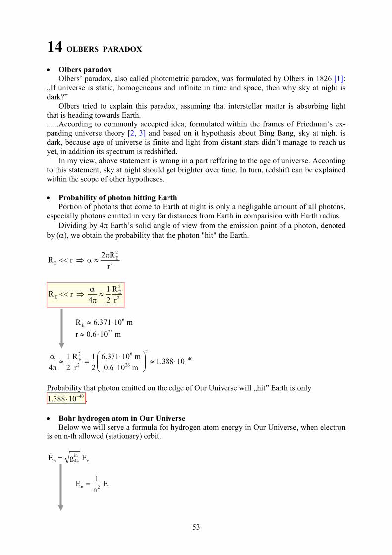
53

14 OLBERS PARADOX

• Olbers paradox Olbers’ paradox, also called photometric paradox, was formulated by Olbers in 1826 [1]:

„If universe is static, homogeneous and infinite in time and space, then why sky at night is

dark?”

Olbers tried to explain this paradox, assuming that interstellar matter is absorbing light

that is heading towards Earth.

......According to commonly accepted idea, formulated within the frames of Friedman’s ex-

panding universe theory [2, 3] and based on it hypothesis about Bing Bang, sky at night is

dark, because age of universe is finite and light from distant stars didn’t manage to reach us

yet, in addition its spectrum is redshifted.

In my view, above statement is wrong in a part reffering to the age of universe. According

to this statement, sky at night should get brighter over time. In turn, redshift can be explained

within the scope of other hypotheses.

• Probability of photon hitting Earth Portion of photons that come to Earth at night is only a negligable amount of all photons,

especially photons emitted in very far distances from Earth in comparision with Earth radius.

Dividing by 4π Earth’s solid angle of view from the emission point of a photon, denoted

by (α), we obtain the probability that the photon "hit" the Earth.

2

2

EE

r

R2 r R

π≈α⇒<<

2

2

EE

r

R

2

1

4 r R ≈

πα

⇒<<

m 10371.6R 6

E ⋅≈

m 106.0r 26⋅≈

40

2

26

6

2

2

E 10388.1m 106.0

m 10371.6

2

1

r

R

2

1

4

−⋅≈

⋅⋅

=≈π

α

Probability that photon emitted on the edge of Our Universe will „hit” Earth is only4010388.1 −⋅ .

• Bohr hydrogen atom in Our Universe Below we will serve a formula for hydrogen atom energy in Our Universe, when electron

is on n-th allowed (stationary) orbit.

n

in

44n E gE =

12n E n

1E =

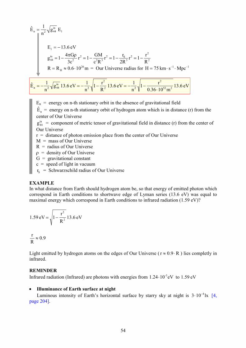
54

1

in

442n E gn

1E =

eV 13.6 E1 −=

2

22

3

S2

32

2

2

in

44R

r1r

2R

r1r

Rc

GM1r

3c

G41g −=−=−=

ρπ−=

m106.0RR 26

H ⋅≈= = Our Universe radius for 11 Mpcskm 57H −− ⋅⋅=

eV 13.6 m100.36

r1

n

1eV 13.6

R

r1

n

1eV 13.6 g

n

1E

252

2

22

2

2

in

442n ⋅−−=−−=−=

En = energy on n-th stationary orbit in the absence of gravitational field

nE = energy on n-th stationary orbit of hydrogen atom which is in distance (r) from the

center of Our Universein

44g = component of metric tensor of gravitational field in distance (r) from the center of

Our Universe

r = distance of photon emission place from the center of Our Universe

M = mass of Our Universe

R = radius of Our Universe

ρ = density of Our Universe

G = gravitational constant

c = speed of light in vacuum

Sr = Schwarzschild radius of Our Universe

EXAMPLEIn what distance from Earth should hydrogen atom be, so that energy of emitted photon which

correspond in Earth conditions to shortwave edge of Lyman series (13.6 eV) was equal to

maximal energy which correspond in Earth conditions to infrared radiation (1.59 eV)?

eV 13.6 R

r1 eV 1.59

2

2

−=

9.0R

r≈

Light emitted by hydrogen atoms on the edges of Our Universe ( R0.9r ⋅≈ ) lies completly in

infrared.

REMIDER

Infrared radiation (Infrared) are photons with energies from eV10 24.1 -3⋅ to eV 59.1

• Illuminance of Earth surface at night

Luminous intensity of Earth’s horizontal surface by starry sky at night is lx103 4−⋅ [4,

page 204].

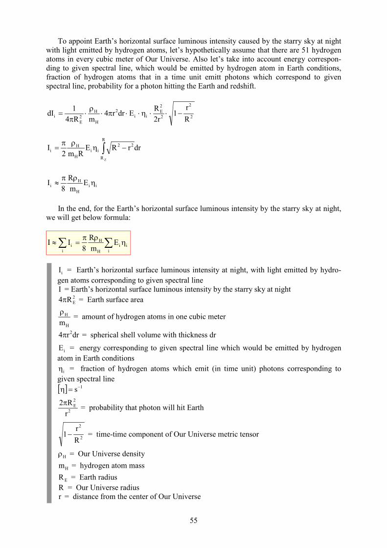
55

To appoint Earth’s horizontal surface luminous intensity caused by the starry sky at night

with light emitted by hydrogen atoms, let’s hypothetically assume that there are 51 hydrogen

atoms in every cubic meter of Our Universe. Also let’s take into account energy correspon-

ding to given spectral line, which would be emitted by hydrogen atom in Earth conditions,

fraction of hydrogen atoms that in a time unit emitt photons which correspond to given

spectral line, probability for a photon hitting the Earth and redshift.

2

2

2

2

Eii

2

H

H

2

E

iR

r1

2r

REdrr4

mR4

1dI −⋅⋅η⋅⋅π⋅

ρ⋅

π=

∫ −ηρπ

=R

R

22

ii

H

Hi

Z

drrRERm2

I

ii

H

Hi E

m

RI η

ρ8π

≈

In the end, for the Earth’s horizontal surface luminous intensity by the starry sky at night,

we will get below formula:

∑∑ ηρ

8π

=≈i

ii

H

H

i

i Em

RII

iI = Earth’s horizontal surface luminous intensity at night, with light emitted by hydro-

gen atoms corresponding to given spectral line

I = Earth’s horizontal surface luminous intensity by the starry sky at night2

ER4π = Earth surface area

H

H

m

ρ = amount of hydrogen atoms in one cubic meter

drr4 2π = spherical shell volume with thickness dr

iE = energy corresponding to given spectral line which would be emitted by hydrogen

atom in Earth conditions

iη = fraction of hydrogen atoms which emit (in time unit) photons corresponding to

given spectral line

[ ] 1s−=η

2

2

E

r

R2π = probability that photon will hit Earth

2

2

R

r1− = time-time component of Our Universe metric tensor

Hρ = Our Universe density

Hm = hydrogen atom mass

ER = Earth radius

R = Our Universe radius

r = distance from the center of Our Universe

56

Quoted works[1] H. W. M. Olbers: Über die Durchsichtigkeit des Weltraums. Berliner astronomisches

Jahrbuch für das Jahr 1826.

[2] A. Friedman: Über die Krümmung des Raumes. Zeitschrift für Physik 10, 6 (1922) 377-

386.

[3] A. Friedmann: Über die Möglichkeit einer Welt mit konstanter negativer Krümmung desRaumes. Zeitschrift für Physik 21, 5 (1924) 326-332.

[4] Szczepan Szczeniowski: Fizyka doświadczalna. Część IV. Opyka. (Experimental physics.Part IV. Optics.) PWN, Warszawa 1963.

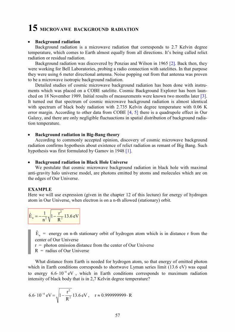
57

15 MICROVAWE BACKGROUD RADIATIO

• Background radiation Background radiation is a microwave radiation that corresponds to 2.7 Kelvin degree

temperature, which comes to Earth almost equally from all directions. It’s being called relict

radiation or residual radiation.

Background radiation was discovered by Penzias and Wilson in 1965 [2]. Back then, they

were working for Bell Laboratories, probing a radio connection with satelittes. In that purpose

they were using 6 meter directional antenna. Noise popping out from that antenna was proven

to be a microwave isotropic background radiation.

Detailed studies of cosmic microwave background radiation has been done with instru-

ments which was placed on a COBE satelitte. Cosmic Background Explorer has been laun-

ched on 18 November 1989. Initial results of measurements were known two months later [3].

It turned out that spectrum of cosmic microwave background radiation is almost identical

with spectrum of black body radiation with 2.735 Kelvin degree temperature with 0.06 K

error margin. According to other data from COBE [4, 5] there is a quadrupole effect in Our

Galaxy, and there are only negligible fluctuactions in spatial distribution of background radia-

tion temperature.

• Background radiation in Big-Bang theory According to commonly accepted opinion, discovery of cosmic microwave background

radiation confirms hypothesis about existence of relict radiation as remant of Big Bang. Such

hypothesis was first formulated by Gamov in 1948 [1].

• Background radiation in Black Hole Universe We postulate that cosmic microwave background radiation in black hole with maximal

anti-gravity halo universe model, are photons emitted by atoms and molecules which are on

the edges of Our Universe.

EXAMPLEHere we will use expression (given in the chapter 12 of this lecture) for energy of hydrogen

atom in Our Universe, when electron is on a n-th allowed (stationary) orbit.

eV 13.6 R

r1

n

1E

2

2

2n −−=

nE = energy on n-th stationary orbit of hydrogen atom which is in distance r from the

center of Our Universe

r = photon emission distance from the center of Our Universe

R = radius of Our Universe

What distance from Earth is needed for hydrogen atom, so that energy of emitted photon

which in Earth conditions corresponds to shortwave Lyman series limit (13.6 eV) was equal

to energy eV 10 6.6 4−⋅ , which in Earth conditions corresponds to maximum radiation

intensity of black body that is in 2,7 Kelvin degree temperature?

eV 13.6 R

r1 eV 10 6.6

2

2

4 −=⋅ − , R999999999.0r ⋅≈

58

REMIDIG

Microwaves correspond to photons with energies from eV1014.4 6−⋅ to eV1024.1 3−⋅ .

Quoted works[1] G. Gamow: The Evolution of the Universe. Nature 162, 4122 (October 30, 1948) 680-682.

[2] A. A. Penzias and R. W. Wilson: A Measurement of Excess Antenna Temperature at 4080MHz. Astrophysical Journal 142 (07/1965) 419-421.

[3] COBE Group: J. C. Mather and his co-workers: A Preliminary Measurements of theCosmic Microwave Background Spectrum by the Cosmic Background Explorer (COBE)Satellite. Astrophysical Journal Letters 354 (May 10, 1990) L37-L40.

[4] COBE Group: G. F. Smoot and his co-workers: First results of the COBE satellitemeasurement of the anisotropy of the cosmic microwave background radiation. Advances in

Space Research 11, 2 (1991) 193-205.

[5] COBE Group: G. F. Smoot and his co-workers: Structure in the COBE differentialmicrowave radiometer first-year maps. Astrophysical Journal 396, 1 (September 1, 1992) L1-

L5.

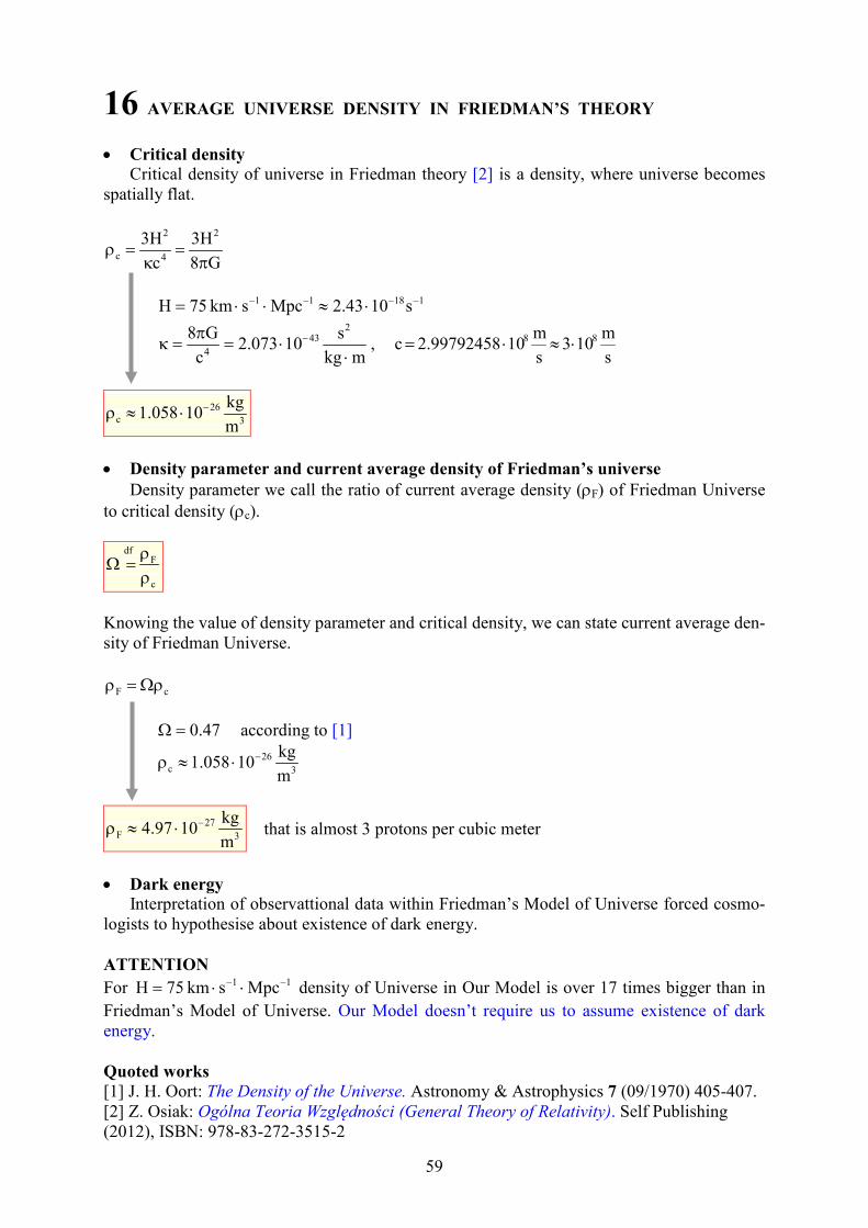
59

16 AVERAGE UIVERSE DESITY I FRIEDMA’S THEORY

• Critical density Critical density of universe in Friedman theory [2] is a density, where universe becomes

spatially flat.

G8

3H

c

3H 2

4

2

c π=

κ=ρ

11811 s102.43Mpcskm 57H −−−− ⋅≈⋅⋅=

mkg

s10073.2

c

G8 243

4 ⋅⋅=

π=κ − ,

s

m103

s

m10 2.99792458c 88 ⋅≈⋅=

3

26

cm

kg10058.1 −⋅≈ρ

• Density parameter and current average density of Friedman’s universe

Density parameter we call the ratio of current average density (ρF) of Friedman Universe

to critical density (ρc).

c

Fdf

ρρ

=Ω

Knowing the value of density parameter and critical density, we can state current average den-

sity of Friedman Universe.

cF Ωρ=ρ

47.0=Ω according to [1]

3

26

cm

kg10058.1 −⋅≈ρ

3

27

Fm

kg1097.4 −⋅≈ρ that is almost 3 protons per cubic meter

• Dark energy Interpretation of observattional data within Friedman’s Model of Universe forced cosmo-

logists to hypothesise about existence of dark energy.

ATTETIO

For 11 Mpcskm 57H −− ⋅⋅= density of Universe in Our Model is over 17 times bigger than in

Friedman’s Model of Universe. Our Model doesn’t require us to assume existence of dark

energy.

Quoted works[1] J. H. Oort: The Density of the Universe. Astronomy & Astrophysics 7 (09/1970) 405-407.

[2] Z. Osiak: Ogólna Teoria Względności (General Theory of Relativity). Self Publishing

(2012), ISBN: 978-83-272-3515-2

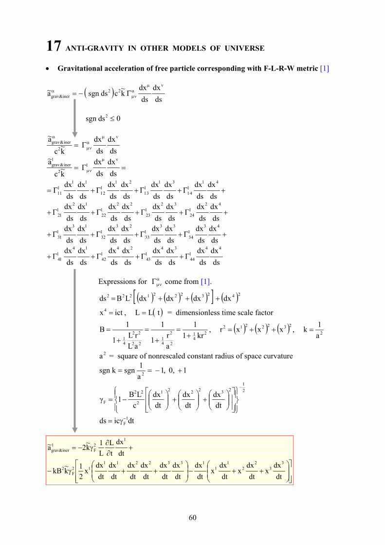
60

17 ATI-GRAVITY I OTHER MODELS OF UIVERSE

• Gravitational acceleration of free particle corresponding with F-L-R-W metric [1]

( )ds

dx

ds

dxk~

c dssgn a~ 22

&inergrav

νµαµν

α Γ −=

0dssgn 2 ≤

ds

dx

ds

dx

k~

c

a~

2

iner&grav

νµαµν

α

Γ =

=Γ =νµ

1µν

1

ds

dx

ds

dx

k~

c

a~

2

iner&grav

+Γ+Γ+Γ+Γ=41

114

31113

21112

11111

ds

dx

ds

dx

ds

dx

ds

dx

ds

dx

ds

dx

ds

dx

ds

dx

+Γ+Γ+Γ+Γ+42

124

32123

22122

12121

ds

dx

ds

dx

ds

dx

ds

dx

ds

dx

ds

dx

ds

dx

ds

dx

+Γ+Γ+Γ+Γ+43

134

33133

23132

13131

ds

dx

ds

dx

ds

dx

ds

dx

ds

dx

ds

dx

ds

dx

ds

dx

ds

dx

ds

dx

ds

dx

ds

dx

ds

dx

ds

dx

ds

dx

ds

dx 44144

34143

24142

14141 Γ+Γ+Γ+Γ+

Expressions for αµνΓ come from [1].

( ) ( ) ( )[ ] ( )24232221222 dx dxdxdx LBds +++=

ictx4 = , ( )t LL = = dimensionless time scale factor

2

41

2

2

41

22

22

41

kr1

1

a

r1

1

aL

rL1

1B

+=

+=

+= , ( ) ( ) ( )2322212 xxxr ++= ,

2a

1k =

2a = square of nonrescaled constant radius of space curvature

1 ,0 ,1 a

1sgn ksgn

2+−==

2

1

23

22

21

2

22

Fdt

dx

dt

dx

dt

dx

c

LB1γ

−

+

+

−=

dticds 1

F

−γ=

++−

++γ−

+∂∂

γ−=

dt

dxx

dt

dxx

dt

dxx

dt

dx

dt

dx

dt

dx

dt

dx

dt

dx

dt

dx

dt

dxx

2

1k~

kB

dt

dx

t

L

L

1 k

~2a~

3

3

2

2

1

1

1332211

12

F

2

1

2

F

1

&inergrav

61

Now let’s determine physical component of gravitational acceleration of free particle in spa-

cetime with F-L-R-W metric.

αα = &inergrav11&inergrav a~ ga~

22

11 LBg =

αα = iner&graviner&grav a~ BLa~

++−

++γ−

+∂∂

γ−=

dt

dxx

dt

dxx

dt

dxx

dt

dx

dt

dx

dt

dx

dt

dx

dt

dx

dt

dx

dt

dxx

2

1k~

LkB

dt

dx

t

LB k

~2a~

3

3

2

2

1

1

1332211

12

F

3

1

2

F

1

&inergrav

In case of spatially flat spacetime (k = 0):

1k~

,0t

L ,

dt

dx

t

L k

~2a~ 2

F

1

2

F

1

iner&grav +=>∂∂

γ∂∂

γ−=

Let’s notice, that

0a~ 0dt

dx1

iner&grav

1

<⇒> 0a~ 0dt

dx1

iner&grav

1

>⇒<

From the relation between signs of velocity components and gravitational acceleration of free

particle, emerges that occurrance of gravity or anti-gravity depends on the velocity direction

of test particle in spatially flat Friedman Universe.

• Gravitational acceleration of free particle corresponding with metric of simple modelof expanding spacetime [1]

( )ds

dx

ds

dxk~

c dssgn a~ 22

&inergrav

νµαµν

α Γ −=

0dssgn 2 ≤

ds

dx

ds

dx

k~

c

a~

2

iner&grav

νµαµν

α

Γ =

=Γ =νµ

1µν

1

ds

dx

ds

dx

k~

c

a~

2

&inergrav

+Γ+Γ+Γ+Γ=41

114

31113

21112

11111

ds

dx

ds

dx

ds

dx

ds

dx

ds

dx

ds

dx

ds

dx

ds

dx

+Γ+Γ+Γ+Γ+42

124

32123

22122

12121

ds

dx

ds

dx

ds

dx

ds

dx

ds

dx

ds

dx

ds

dx

ds

dx

62

+Γ+Γ+Γ+Γ+43

134

33133

23132

13131

ds

dx

ds

dx

ds

dx

ds

dx

ds

dx

ds

dx

ds

dx

ds

dx

ds

dx

ds

dx

ds

dx

ds

dx

ds

dx

ds

dx

ds

dx

ds

dx 44144

34143

24142

14141 Γ+Γ+Γ+Γ+

Expressions for αµνΓ come from [1].

( ) ( ) ( ) ( )[ ] dxdxdxdx Lds2423222122 +++=

ictx4 = , ( )t LL = = dimensionless time scale factor

2

1

23

22

21

2 dt

dx

dt

dx

dt

dx

c

11γ

−

+

+

−= , dticLds 1−γ=

dt

dx

t

L

L

1 k

~2a~

1

3

21

iner&grav ∂∂

γ−=

Let’s now determine physical component of gravitational acceleration of free particle in spa-

cetime with metric that represents a metric of a simple expanding spacetime model.

αα = &inergrav11&inergrav a~ ga~

2

11 Lg =

αα = iner&graviner&grav a~ La~

1k~

,0t

L

L

1 ,

dt

dx

t

L

L

1 k

~2a~

2

2

1

2

21

iner&grav +=>∂∂

γ∂∂

γ−=

Let’s notice, that

0a~ 0dt

dx1

iner&grav

1

<⇒> 0a~ 0dt

dx1

iner&grav

1

>⇒<

From the relation between signs of velocity components and gravitational acceleration of free

particle, emerges that occurrance of gravity or anti-gravity depends on the velocity direction

of test particle in spacetime with metric that represents a metric of a simple model of expan-

ding spacetime.

Quoted works[1] Z. Osiak: Ogólna Teoria Względności (General Theory of Relativity). Self Publishing

(2012), ISBN: 978-83-272-3515-2

63

18 OUR UIVERSE AS A EISTEI’S SPACE

• Other form of field equations – Our Universe as an Einstein’s space

−κ= αβαβαβ Tg2

1TR ,

mkg

s102.073

c

G8 243

4 ⋅⋅=

π=κ −

0gggggggggggg 433442243223411431132112 ============

44

11g

1g = , 2

22 rg = , θsinrg 22

33 =

2ρcg

2

1 T αααα = ,

2df

ρ2TgT c==∑4

1=ααα

αα,

2cg2

1Tg

2

1T ρ−=− αααααα

0RRRRRRRRRRRR 433442243223411431132112 ============

∂

∂+

∂∂

=2

44

2

44

44

11r

g

2

1

r

g

r

1

g

1R

r

grg1R 44

4422 ∂∂

++−=

∂∂

++−=r

grg 1 θsinR 44

44

2

33

∂

∂+

∂∂

=2

44

2

444444

r

g

2

1

r

g

r

1gR

( )ν≠µ=νµα=κρ−= µναααα ;4,3,2,1,, ,0 R ,gc R 2

21

Spacetime described by above equations, in which every component of Ricci tensor is pro-

portional to adequate component of metric tensor is an Einstein’s space [1]. So spacetime of

Our Universe is an Einstein’s space.

ATTETIOAll mixed components of Ricci tensor are always equal to zero. Set of remaining equations

can be reduced only to two independent variables.

2222

1111

κρ−=

κρ−=

gc R

gc R

2

21

2

21

⇒

2244

44

2

2

44

2

44

cr2

1

r

grg1

c2

1

r

g

2

1

r

g

r

1

ρκ−=∂

∂++−

κρ−=∂

∂+

∂∂

Quoted works[1] А. З. Петров: Пространства Эйнштейна. Физматгиз, Москва 1961.

There is an English translation of the above book:

A. Z. Petrov: Einstein Spaces. Pergamon Press, Oxford 1969.

64

0t

=∂∂E

inin gradk~

ϕ−=E

Gauss law:

ρπ−= G4 div inE

α+α=α graddivdiv AAA

ϕ∆=ϕ∇=ϕ 2grad div

2

2

2

2

2

2

zyx ∂∂

+∂∂

+∂∂

=∆

∆ = Laplace operator

laplacian

19 ASSUMPTIOS

• Main postulates of General Relativity General Theory of Relativity (General Relativity) studies conclusions that emerge from

assumptions:

1. Maximum speed of signals propagation is the same in every frame of reference.

2. Definitions of physical quantities and physics equations can be formulated in a way so that

their overall forms are the same in all frames of reference.

3. Spacetime metric depends on density distribution of source masses.

4. Inertial mass is equal to gravitational mass.

• 2-potential nature of stationary gravitational field Stationary gravitational field is a 2-potential field:

~

−

+=

source mass a of inside 1

source mass a of outside 1k

• Poisson’s equation and 2-potential nature of stationary gravitational field

• Signes of right sides of Poisson’s and Einstein’s equations and boundary conditions In Newton's theory of gravity, boundary conditions for the gravitational potentials

0 lim R,r

0 lim R,r0

ex

r

in

0r

=ϕ≥

=ϕ<≤

∞→

→

in spherical coordinates correspond to the following forms of Poisson’s equation

0t

=∂∂E

, 0rot =E

0grad rot =ϕ

ininin gradkgrad ϕ−=ϕ=~ E , Rr0 <≤ , 0 lim in

0r=ϕ

→

exexex gradkgrad ϕ−=ϕ−=~ E , Rr ≥ , 0 lim ex

r=ϕ

∞→

⇒

Poisson’s equation

ρπ−=ρπ=ϕ∆ G4Gk~

4in

In empty space, outside of a mass source, right side of

Poisson’s equation is equal to zero.

Laplace’s equation

0ex =ϕ∆

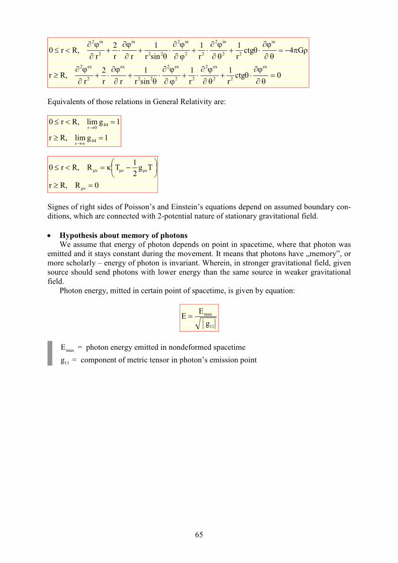
65

0

ctgr

1

r

1

sinr

1

r r

2

r R,r

ρG4

ctgr

1

r

1

sinr

1

r r

2

r R,r0

ex

22

ex2

22

ex2

22

ex

2

ex2

in

22

in2

22

in2

22

in

2

in2

=θ∂

ϕ∂⋅θ+

θ∂

ϕ∂⋅+

ϕ∂

ϕ∂⋅

θ+

∂

ϕ∂⋅+

∂

ϕ∂≥

π−=θ∂

ϕ∂⋅θ+

θ∂

ϕ∂⋅+

ϕ∂

ϕ∂⋅

θ+

∂

ϕ∂⋅+

∂

ϕ∂<≤

Equivalents of those relations in General Relativity are:

1g lim R,r

1g lim R,r0

44r

440r

=≥

=<≤

∞→

→

0R R,r

Tg2

1TκR R,r0

µν

µνµνµν

=≥

−=<≤

Signes of right sides of Poisson’s and Einstein’s equations depend on assumed boundary con-

ditions, which are connected with 2-potential nature of stationary gravitational field.

• Hypothesis about memory of photons We assume that energy of photon depends on point in spacetime, where that photon was

emitted and it stays constant during the movement. It means that photons have „memory”, or

more scholarly – energy of photon is invariant. Wherein, in stronger gravitational field, given

source should send photons with lower energy than the same source in weaker gravitational

field.

Photon energy, mitted in certain point of spacetime, is given by equation:

11

max

g

EE =

maxE = photon energy emitted in nondeformed spacetime

11g = component of metric tensor in photon’s emission point

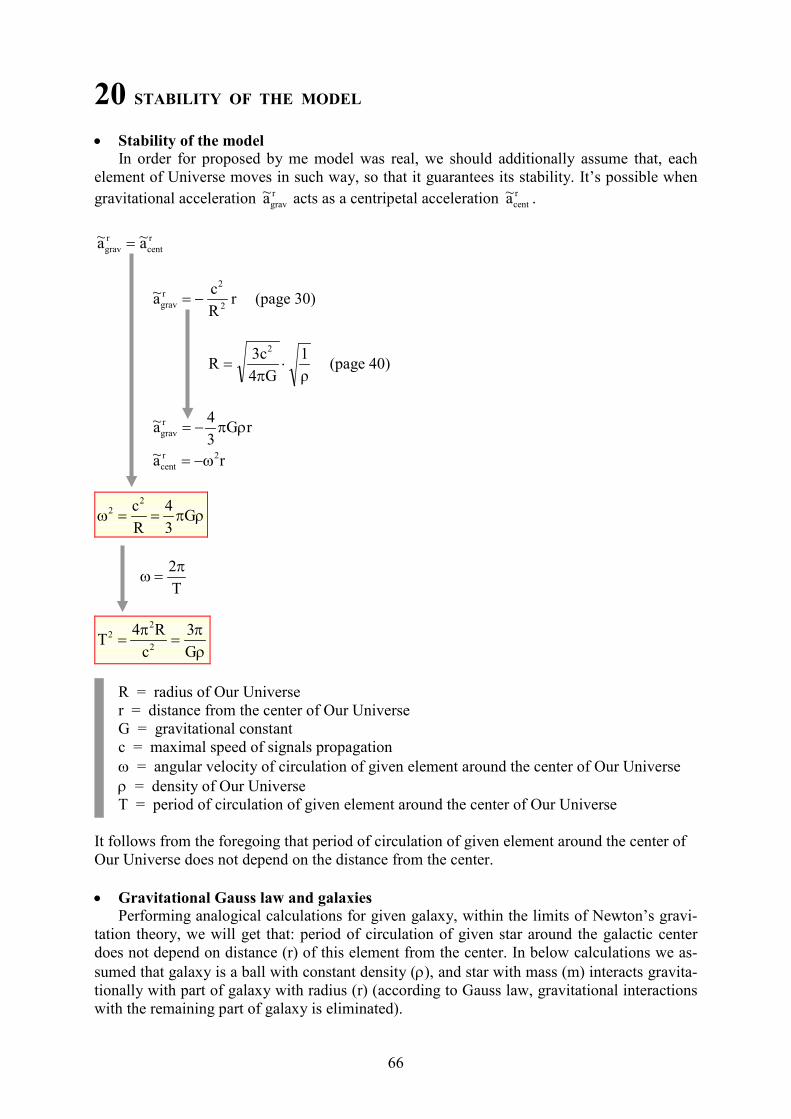
66

20 STABILITY OF THE MODEL

• Stability of the model In order for proposed by me model was real, we should additionally assume that, each

element of Universe moves in such way, so that it guarantees its stability. It’s possible when

gravitational acceleration r

grava~ acts as a centripetal acceleration r

centa~ .

r

cent

r

grav a~a~ =

r R

c a~

2

2r

grav −= (page 30)

ρ

1

G4

3cR

2

⋅π

= (page 40)

rG3

4a~ r

grav ρπ−=

ra~ 2r

cent ω−=

ρπ==ω G3

4

R

c22

T

2π=ω

ρπ

=π

=G

3

c

R4T

2

22

R = radius of Our Universe

r = distance from the center of Our Universe

G = gravitational constant

c = maximal speed of signals propagation

ω = angular velocity of circulation of given element around the center of Our Universe

ρ = density of Our Universe

T = period of circulation of given element around the center of Our Universe

It follows from the foregoing that period of circulation of given element around the center of

Our Universe does not depend on the distance from the center.

• Gravitational Gauss law and galaxies Performing analogical calculations for given galaxy, within the limits of Newton’s gravi-

tation theory, we will get that: period of circulation of given star around the galactic center

does not depend on distance (r) of this element from the center. In below calculations we as-

sumed that galaxy is a ball with constant density (ρ), and star with mass (m) interacts gravita-

tionally with part of galaxy with radius (r) (according to Gauss law, gravitational interactions

with the remaining part of galaxy is eliminated).

67

The force of gravity gravF act as centripetal force centF .

centgrav FF =

2grav

r

GMmF = (Newton’s gravity force)

ρπ= 3r3

4M

Gmr3

4Fgrav π=

rmF 2

cent ω= (centripetal force)

ρπ=ω G3

42

T

2π=ω

ρπ

=G

3T2

R = radius of galaxy

r = distance from the galaxy center

M = part of galaxy mass with radius r

m = mass of given star

ρ = galaxy density

G = gravitational constant

ω = angular velocity of circulation of given star around the galactic center

T = period of circulation of given star around the galactic center

68

21 MAI RESULTS

• Hypothesis about existence of anti-gravity Quadratic differential form of spacetime can be interpreted as square of spacetime distan-

ces of two points, called „events”, that are located very close to each other in spacetime. Spa-

cetime distance between two events is not a magnitude that can be directly measured, because

we don’t have „4 dimensional rulers”. Also, depending on the sign of the quadratic differen-

tial form of spacetime, spacetime distances can be imaginary or real.

• Black hole with maximal anti-gravity halo It has been shown that exterior (vacuum) solution of gravitational field equations, which

has been served by Schwarzschild in 1916, hides anti-gravity. Spatial radius of black hole

with maximal anti-gravity halo is equal to half of Schwarzschild radius. Space outside of the

black hole with maximal anti-gravity halo consists of two layers, in first ( SS rr r5.0 <≤ ) anti-

gravity occures, in second ( Srr > ) – gravity. Thickness of anti-gravity layer is equal to the

spatial radius of black hole with maximal anti-gravity layer. Inside this anti-gavity layer, ac-

celeration is pointed away from the center of mass source, in gravitational part – to the center.

• Hypothesis about 2-potential nature of stationary gravitational field Acceptance of hypothesis about 2-potential nature of stationary gravitational field made it

possible to find interior solution for field equations that correspond with gravitational Gauss

law and also made it possible to accomplish a modification of field equations.

• Field equations contain equations of motion Has been justified that equations of motion of free test particle are contained in gravitatio-

nal field equations (that is in spacetime metric equations).

• Black Hole model of Our Universe Our Universe can be treated as a gigantic homogeneous black hole with spatial radius

equal to half of Schwarzschild radius. It is isolated from the rest of universe with an area of

spacetime where anti-gravity occurres.

Our Galaxy, together with Solar system and Earth, which in cosmological scales can be

viewed only as a small point, should be located near the center of Black Hole Universe. Let’s

emphasize again, that in the center of black hole, gravitational acceleration of free test partic-

le, ignoring local gravitational fields, is equal to zero. In other words: black hole is not crea-

ting gravitational field in its center.

The gravitational field is stronger, the space is more stretched. For Earth observer, the

local space with increasing distance from Earth is becoming less stretched. In cosmic scale we

have different situation: the further away from the Earth, the space is more stretched.

Sign change (from negative to positive) of quadratic differential form of spacetime means

transition from gravity to anti-gravity.

GRAVITY0ds2 ⇔<GRAVITY-ANTI0ds2 ⇔>

69

• Size of Our Universe

For 11 Mpcskm 57H −− ⋅⋅= radius of Our Universe has value:

years ightl 10 6.31m106.0R 926 ⋅≈⋅≈ In a distance from the center of Earth approximate equal to:

yearslight 236300yearslight 10363.2m10245.2r 521

0 =⋅≈⋅≈

redshift measured in regard to our planet, changes its sign from negative to positive.

Light that comes to Earth from Our Galaxy (which radius is around 50,000 light years and

thickness is around 12,000 light years) should be shifted towards violet in regard to light that

is emitted on Earth surface. Wherein negative value of redshift should depend on direction of

observation.

• Density of Our Universe

For 11 Mpcskm 57H −− ⋅⋅= density of Universe in Our Model is over 17 times bigger than

in Friedman Universe Model and is: 327 mkg1059.48ρ −− ⋅⋅= , that almost 51 protons per cu-

bic meter.

ATTETIOOur Model doesn’t require assumption about existence of dark energy.

• Photon paradox Commonly accepted assumption, that photon energy doesn’t depend on place of emis-

sion, leads to a paradox. In spacetimes other than conformally flat, length and oscillation pe-

riod of electromagnetic wave modelled by photon depends in different way on respective

components of metric tensor. However photon energy depends on length or period in analogi-

cal way (that is inversely proportional).

• Hypothesis about memory of photons Within the model of Our Universe as a black hole with maximum anti-gravity halo, hypo-

thesis about memory of photons explains:

1. photon paradox,

2. Olbers’ photometric paradox,

3. redshift dependence on the distance from Earth:

A. nonlinear growth of redshift for big distances from Earth,

B. existence of distance from Earth, where redshift changes its sign from negative to positi-

ve,

4. origin of cosmic microwave background radiation,

5. why hypothesis about existence of dark energy is unnecessary.

ATTETIOIt should be highlighted that Pound-Rebka experiment doesn’t exlude hypothesis about me-

mory of photons.

• Our Universe is an Einstein’s space It has been shown that field equations which are modelling Our Universe and black hole

with maximum anti-gravity halo can be brought to a form which describe so called Einstein’s

space.

• Anti-gravity in other cosmological models From the relation between signs of components of velocity and gravitational acceleration

of free test particle emerges that occurance of gravity or anti-gravity depends on the direction

of velocity of test particle in spatiallly flat Friedman Universe as well as in spacetime with

metric of a simple expanding spacetime model [1].

70

• ew tests of General Relativity To show in Earth conditions, existence of a black holes with anti-gravity halo and also 2-

potential nature of gravitational field, we need to measure ratio of distance passed by light to

the time of flight, in a vertically positioned vacuum cylinder, right under and right above the

surface of Earth (of the sea level). If the difference of squares of those measurements will be

equal to the square of escape speed, then it will prove existence of black holes with anti-gravi-

ty halo. This experiment would be a new test of General Theory of Relativity.

If Our Universe is a black hole with anti-gravity halo, then in the distance from the center

of Earth approximately equal to 236,000 light years redshift measured in regard to Our Planet

changes its sign from negative to positive. Light that comes to Earth from Our Galaxy (radius

of Milky Way is around 50,000 light years and its thickness is around 12,000 light years)

should be shifted towards violet in regard to light that is emitted on Earth. Wherein negative

value of redshift should depend on direction of observation

Quoted works[1] Z. Osiak: Ogólna Teoria Względności (General Theory of Relativity). Self Publishing

(2012), ISBN: 978-83-272-3515-2

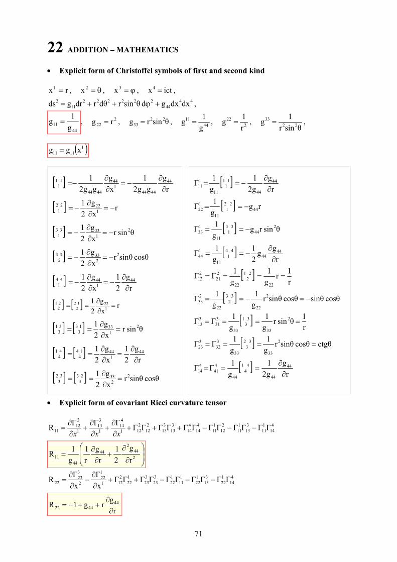
71

22 ADDITIO – MATHEMATICS

• Explicit form of Christoffel symbols of first and second kind

rx1 = , θ=2x , ϕ=3x , ictx4 = ,

44

44

222222

11

2 dxdxgd θsinrdθrdrgds +ϕ++= ,

44

11g

1g = , 2

22 rg = , θsinrg 22

33 = , 44

11

g

1g = ,

2

22

r

1g = ,

θsinr

1g

22

33 = ,

( )1

1111 xgg =

• Explicit form of covariant Ricci curvature tensor

4

14

1

11

3

13

1

11

2

12

1

11

4

14

4

14

3

13

3

13

2

12

2

121

4

14

1

3

13

1

2

1211R ΓΓ−ΓΓ−ΓΓ−ΓΓ+ΓΓ+ΓΓ+

∂Γ∂

+∂Γ∂

+∂Γ∂

=xxx

∂

∂+

∂∂

=2

44

2

44

44

11r

g

2

1

r

g

r

1

g

1R

4

14

1

22

3

13

1

22

1

11

1

22

3

23

3

23

1

22

2

121

1

22

2

3

2322

x

Γ

x

ΓR ΓΓ−ΓΓ−ΓΓ−ΓΓ+ΓΓ+

∂∂

−∂∂

=

r

grg1R 44

4422 ∂∂

++−=

[ ]r

g

g2

1

g

1 44

44

1 1

1

11

1

11 ∂∂

−==Γ

[ ] rg g

144

2 2

1

11

1

22 −==Γ

[ ] θsinr g g

1 2

44

3 3

1

11

1

33 −==Γ

[ ]r

gg

2

1

g

1 4444

4 4

1

11

1

44 ∂∂

−==Γ

[ ]r

1r

g

1

g

1

22

2 1

2

22

2

21

2

12 ===Γ=Γ

[ ] cosθ sinθcosθ sinθrg

1

g

1 2

22

3 3

2

22

2

33 −=−==Γ

[ ]r

1θsinr

g

1

g

1 2

33

3 1

3

33

3

31

3

13 ===Γ=Γ

[ ] ctgθcosθ sinθrg

1

g

1 2

33

3 2

3

33

3

32

3

23 ===Γ=Γ

[ ]r

g

2g

1

g

1 44

44

4 1

4

44

4

41

4

14 ∂∂

==Γ=Γ

[ ]r

g

gg2

1

x

g

gg2

1 44

4444

1

44

4444

1 1

1 ∂∂

−=∂∂

−=

[ ] rx

g

2

1

1

222 2

1 −=∂∂

−=

[ ] θsinr x

g

2

1 2

1

333 3

1 −=∂∂

−=

[ ] cosθ sinθrx

g

2

1 2

2

333 3

2 −=∂∂

−=

[ ]r

g

2

1

x

g

2

1 44

1

444 4

1 ∂∂

−=∂∂

−=

[ ] [ ] rx

g

2

1

1

221 2

2

2 1

2 =∂∂

==

[ ] [ ] θsinr x

g

2

1 2

1

331 3

3

3 1

3 =∂∂

==

[ ] [ ]r

g

2

1

x

g

2

1 44

1

441 4

4

4 1

4 ∂∂

=∂∂

==

[ ] [ ] cosθ sinθrx

g

2

1 2

2

332 3

3

3 2

3 =∂∂

==

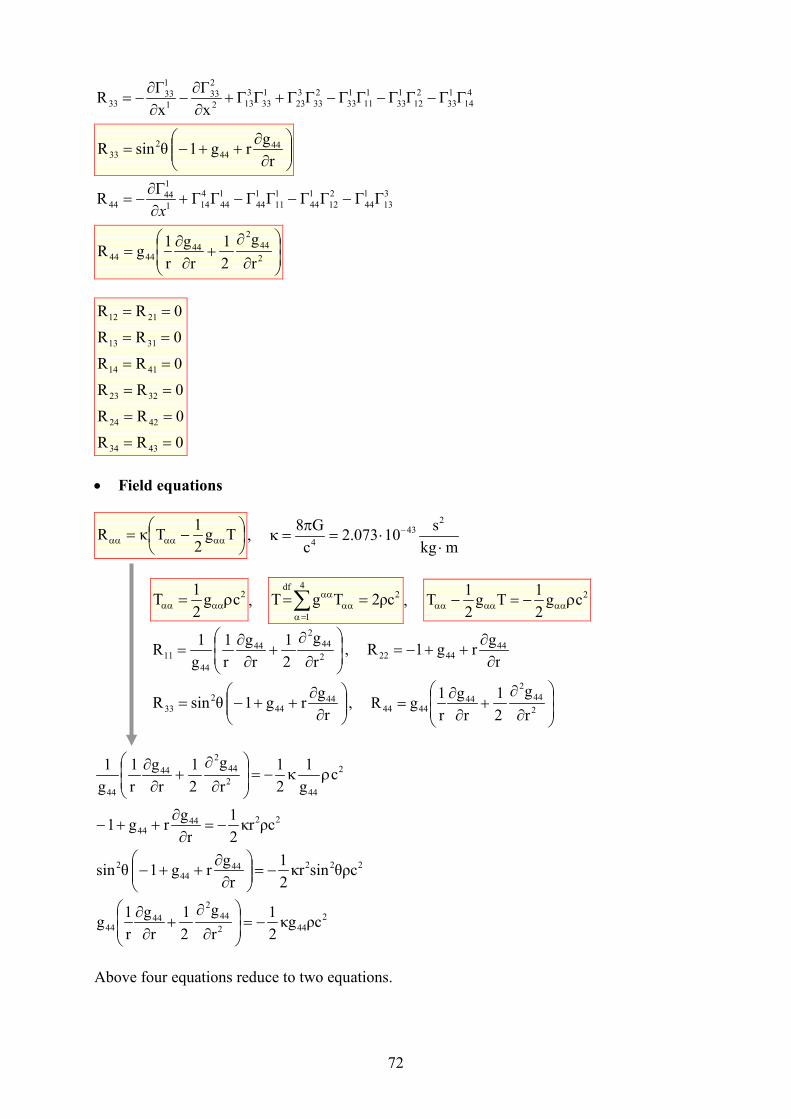
72

4

14

1

33

2

12

1

33

1

11

1

33

2

33

3

23

1

33

3

132

2

33

1

1

3333

x

Γ

x

ΓR ΓΓ−ΓΓ−ΓΓ−ΓΓ+ΓΓ+

∂∂

−∂∂

−=

∂∂

++−=r

grg 1 θsinR 44

44

2

33

3

13

1

44

2

12

1

44

1

11

1

44

1

44

4

141

1

4444 ΓΓΓΓΓΓΓΓR −−−+

∂Γ∂

−=x

∂

∂+

∂∂

=2

44

2

444444

r

g

2

1

r

g

r

1gR

0RR

0RR

0RR

0RR

0RR

0RR

4334

4224

3223

4114

3113

2112

==

==

==

==

==

==

• Field equations

−= αααααα Tg2

1TκR ,

mkg

s10073.2

c

G8 243

4 ⋅⋅=

π=κ −

2cg

2

1T ρ= αααα ,

2df

ρ2TgT c==∑4

1=ααα

αα,

2cg2

1Tg

2

1T ρ−=− αααααα

∂

∂+

∂∂

=2

44

2

44

44

11r

g

2

1

r

g

r

1

g

1R ,

r

grg1R 44

4422 ∂∂

++−=

∂∂

++−=r

grg 1 θsinR 44

44

2

33 ,

∂

∂+

∂∂

=2

44

2

444444

r

g

2

1

r

g

r

1gR

2

44

2

44

2

44

44

cg

1

2

1

r

g

2

1

r

g

r

1

g

1ρκ−=

∂

∂+

∂∂

224444 ρcκr

2

1

r

grg1 −=

∂∂

++−

2224444

2 θρcsinκr2

1

r

grg 1 θsin −=

∂∂

++−

2

442

44

2

4444 ρcκg

2

1

r

g

2

1

r

g

r

1g −=

∂

∂+

∂∂

Above four equations reduce to two equations.

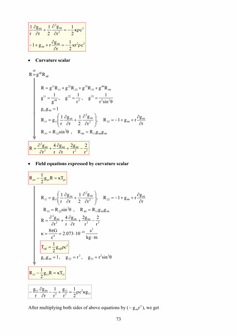
73

224444

2

2

44

2

44

cr2

1

r

grg1

c2

1

r

g

2

1

r

g

r

1

ρκ−=∂

∂++−

κρ−=∂

∂+

∂∂

• Curvature scalar

αβ

αβdf

RgR =

44

44

33

33

22

22

11

11 RgRgRgRgR +++=

44

11

g

1g = ,

2

22

r

1g = ,

θsinr

1g

22

33 =

1gg 4411 =

∂

∂+

∂∂

=2

44

2

441111

r

g

2

1

r

g

r

1gR ,

r

grg1R 44

4422 ∂∂

++−=

sinRR 2

2233 θ= , 44441144 ggRR =

22

4444

2

44

2

r

2

r

2g

r

g

r

4

r

gR −+

∂∂

+∂

∂=

• Field equations expressed by curvature scalar

µνµνµν κTRg2

1R =−

∂

∂+

∂∂

=2

44

2

441111

r

g

2

1

r

g

r

1gR ,

r

grg1R 44

4422 ∂∂

++−=

sinRR 2

2233 θ= , 44441144 ggRR =

22

4444

2

44

2

r

2

r

2g

r

g

r

4

r

gR −+

∂∂

+∂

∂=

mkg

s10073.2

c

G8 243

4 ⋅⋅=

π=κ −

2ρcg

2

1T αβαβ =

1gg 4411 = , 2

22 rg = , θsinrg 22

33 =

111111 κTRg2

1R =−

112

11

2

4411 gc2

1

r

g

r

1

r

g

r

gκρ=+−

∂∂

− 2

After multiplying both sides of above equations by ( 2

44rg− ), we get

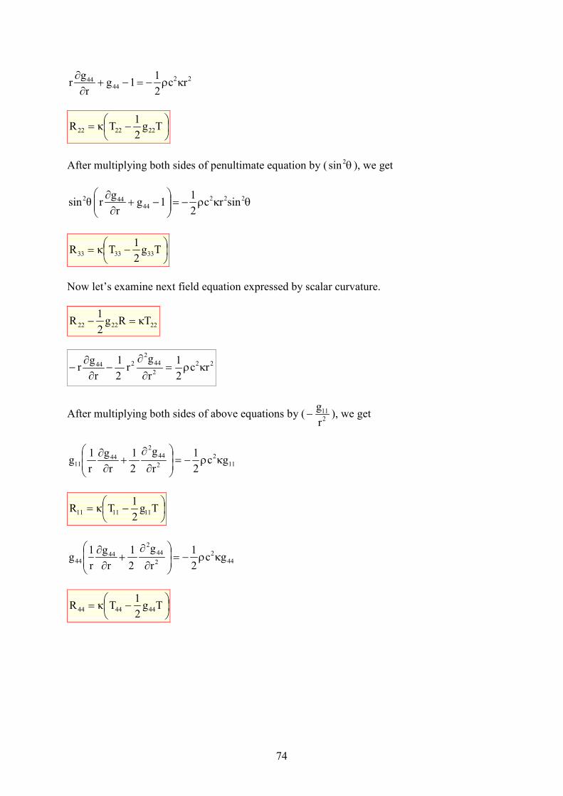
74

22κρ−=−+∂

∂rc

2

11g

r

gr 44

44

−= 222222 Tg2

1TκR

After multiplying both sides of penultimate equation by ( θ2sin ), we get

θκρ−=

−+

∂∂ 222

44442 sinrc

2

11g

r

gr θsin

−= 333333 Tg2

1TκR

Now let’s examine next field equation expressed by scalar curvature.

222222 κTRg2

1R =−

22

2

44

2

244 rc2

1

r

gr

2

1

r

gr κρ=

∂

∂−

∂∂

−

After multiplying both sides of above equations by (2

11

r

g− ), we get

11

2

2

44

2

4411 gc

2

1

r

g

2

1

r

g

r

1g κρ−=

∂

∂+

∂∂

−= 111111 Tg2

1TκR

44

2

2

44

2

4444 gc

2

1

r

g

2

1

r

g

r

1g κρ−=

∂

∂+

∂∂

−= 444444 Tg2

1TκR

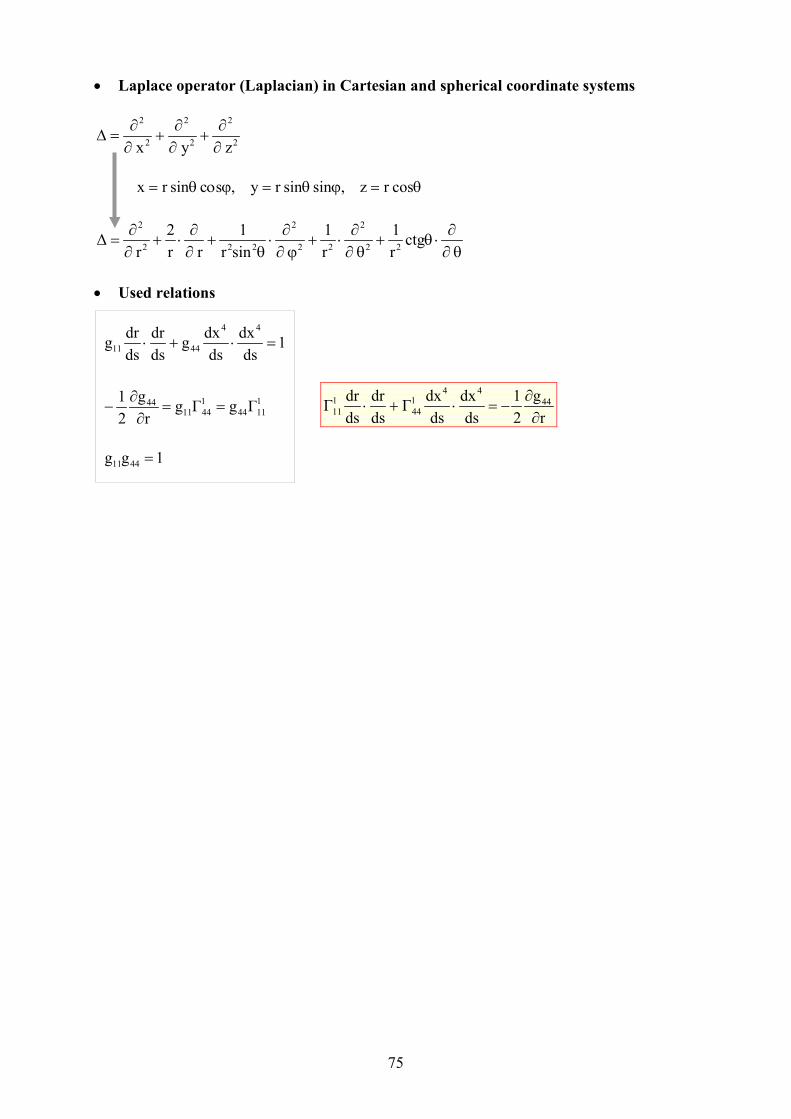
75

• Laplace operator (Laplacian) in Cartesian and spherical coordinate systems

2

2

2

2

2

2

z y x ∂∂

+∂∂

+∂∂

=∆

θ=ϕ θ=ϕο θ= cosr z ,sinsinr y ,scsinr x

θ∂∂

⋅θ+θ∂

∂⋅+

ϕ∂∂

⋅θ

+∂∂

⋅+∂∂

=

ctgr

1

r

1

sinr

1

r r

2

r ∆

22

2

22

2

222

2

• Used relations

1ds

dx

ds

dxg

ds

dr

ds

drg

44

4411 =⋅+⋅

1

1144

1

441144 ΓgΓgr

g

2

1==

∂∂

− r

g

2

1

ds

dx

ds

dxΓ

ds

dr

ds

drΓ 44

441

44

1

11 ∂∂

−=⋅+⋅

1gg 4411 =

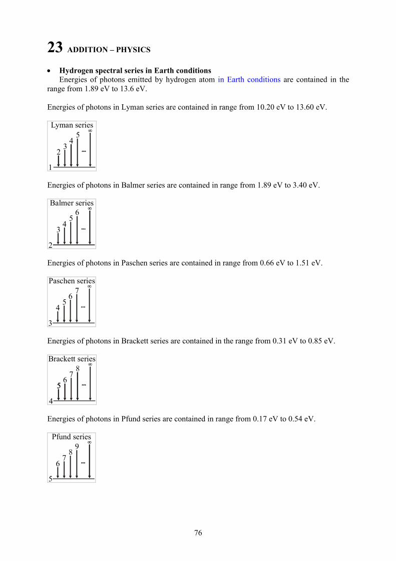
76

23 ADDITIO – PHYSICS

• Hydrogen spectral series in Earth conditions Energies of photons emitted by hydrogen atom in Earth conditions are contained in the

range from 1.89 eV to 13.6 eV.

Energies of photons in Lyman series are contained in range from 10.20 eV to 13.60 eV.

∞

1

23

45

Lyman series

Energies of photons in Balmer series are contained in range from 1.89 eV to 3.40 eV.

∞Balmer series

4

2

3

56

Energies of photons in Paschen series are contained in range from 0.66 eV to 1.51 eV.

∞

3

45

67

Paschen series

Energies of photons in Brackett series are contained in the range from 0.31 eV to 0.85 eV.

∞

4

556

7

Brackett series

Energies of photons in Pfund series are contained in range from 0.17 eV to 0.54 eV.

∞

5

67

9

Pfund series

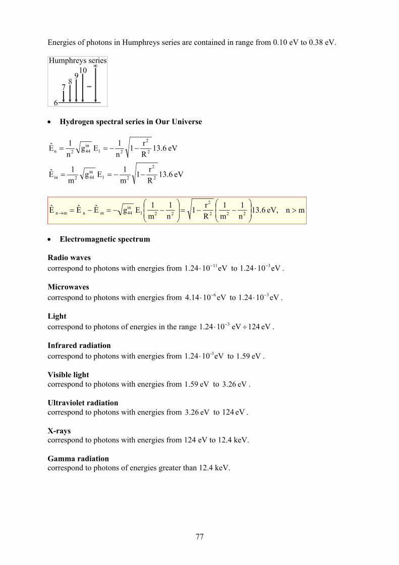
77

Energies of photons in Humphreys series are contained in range from 0.10 eV to 0.38 eV.

∞

6

7

910

Humphreys series

• Hydrogen spectral series in Our Universe

eV 13.6 R

r1

n

1E g

n

1E

2

2

21

in

442n −−==

eV 13.6 R

r1

m

1E g

m

1E

2

2

21

in

442m −−==

mn eV, 13.6 n

1

m

1

R

r1

n

1

m

1E gEEE

222

2

221

in

44m n mn >

−−=

−−=−=→

• Electromagnetic spectrum

Radio waves

correspond to photons with energies from eV1024.1 11−⋅ to eV1024.1 3−⋅ .

Microwaves

correspond to photons with energies from eV1014.4 6−⋅ to eV1024.1 3−⋅ .

Light

correspond to photons of energies in the range Ve 124Ve 1024.1 3 ÷⋅ − .

Infrared radiation

correspond to photons with energies from eV10 24.1 -3⋅ to eV 59.1 .

Visible light

correspond to photons with energies from eV 59.1 to eV 26.3 .

Ultraviolet radiation

correspond to photons with energies from eV 26.3 to eV 241 .

X-rayscorrespond to photons with energies from 124 eV to 12.4 keV.

Gamma radiationcorrespond to photons of energies greater than 12.4 keV.

78

• Choosen concepts, constants and units

Speed of light in vacuum

s

m103

s

m102.99792458c 88 ⋅≈⋅=

Planck’s constant

seV10 4.13566743sJ106.6260693h 1534 ⋅⋅=⋅⋅= −−

Gravitational constant

2

311

2

311

skg

m106.7

skg

m106.6742G

⋅⋅≈

⋅⋅= −−

Einstein’s constant

mkg

s10073.2

c

G8 243

4 ⋅⋅=

π=κ −

Light year (ly), distance passed by light in vacuum during average sun year

m109.5m109.460536ly 1 1515 ⋅≈⋅=

m103.0861pc 16⋅=

s103.1561year 7⋅=

Mass of proton

kg1067262171.1m 27

p

−⋅=

Mass of the Earth

kg106kg105.9736MM 2424

E ⋅≈⋅== ⊕

Mass of the Sun

kg102kg101.9891M 3030

S ⋅≈⋅=

Hubble’s constant unit

s

1100.324

Mpcs

km 19−⋅=⋅

Critical density of Universe in Friedman’s models expresssed by Hubble’s constant (H) and

gravitational constant (G)

G8

3H

c

3H 2

4

2

c π=

κ=ρ

Average radius of the Sun

m100.696R 9

S ⋅=

79

Average radius of the Earth

m106.371R 6

E ⋅=

Radius of Bohr hydrogen atom

m10830.52917720R 10

B

−⋅=

J101.60217653eV 1 19−⋅=

1272

mkg1032.0G4

3c −⋅⋅≈π

, mkg10125.33c

G4 127

2⋅⋅≈

π −−

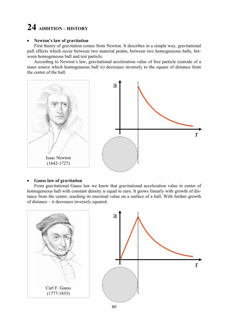
80

24 ADDITIO – HISTORY

• ewton’s law of gravitation First theory of gravitation comes from Newton. It describes in a simple way, gravitational

pull effects which occur between two material points, between two homogeneous balls, bet-

ween homogeneous ball and test particle.

According to Newton’s law, gravitational acceleration value of free particle (outside of a

mass source which homogeneous ball is) decreases inversely to the square of distance from

the center of the ball.

• Gauss law of gravitation From gravitational Gauss law we know that gravitational acceleration value in center of

homogeneous ball with constant density is equal to zero. It grows linearly with growth of dis-

tance from the center, reaching its maximal value on a surface of a ball. With further growth

of distance – it decreases inversely squared.

Isaac Newton

(1642-1727)

Carl F. Gauss

(1777-1855)

81

• Einstein’s General Theory of Relativity General Theory of Relativity (General Relativity) explains gravity as a result of deforma-

tion of spacetime, which depends on density distribution of source masses. The free test parti-

cles move in space along the tracks, which correspond to geodetic lines in spacetime. General

Relativity forces us to revise, inter alia, concepts such as gravitational forces, the forces of

inertia and inertial frames.

General Relativity was finally formulated by Einstein on

25 November 1915. This theory bases on four postulates:

1. Maximum speed of signals propagation is the same in

every frame of reference.

2. Definitions of physical quantities and physics equations

can be formulated in a way so that their overall forms are

the same in all frames of reference.

3. Spacetime metic depends on density distribution of

source masses.

4. Inertial mass is equal to gravitational mass.

• External (vacuum) Schwarzschild solution

Precise external (vacuum) solution for gravitational field

equations was served by Schwarzschild in 1916:

r

r1

g

1g S

11

44 −== , Rr ≥

M = mass of a homogeneous ball with constant density

R = radius of a ball

2S

c

2GMr = = Schwarzschild radius

Anti-gravity is hidden in this solution.

It is easy to see that, for Srr > sign of quadratic differen-

tial form of spacetime

( ) ( ) ( )24

44

2

11

2dxgdrgds +=

is negative, and for Srr < this sign is positive.

Carl Schwarzschild

(1873-1916)

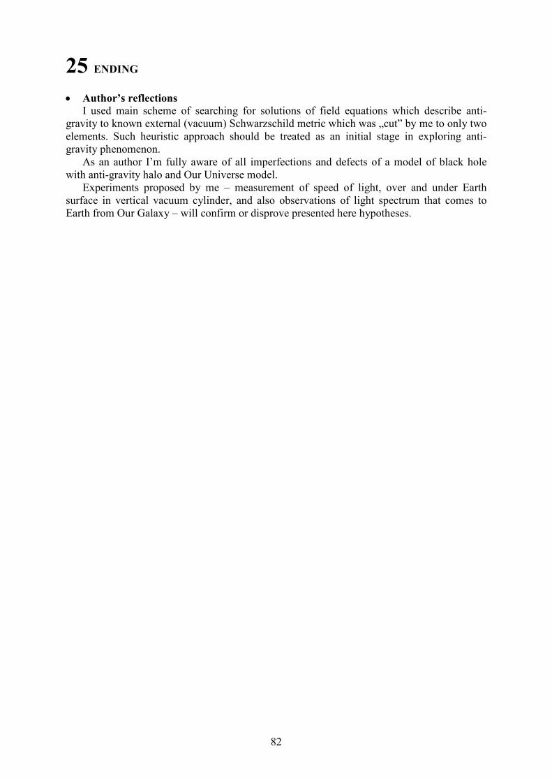
82

25 EDIG

• Author’s reflections I used main scheme of searching for solutions of field equations which describe anti-

gravity to known external (vacuum) Schwarzschild metric which was „cut” by me to only two

elements. Such heuristic approach should be treated as an initial stage in exploring anti-

gravity phenomenon.

As an author I’m fully aware of all imperfections and defects of a model of black hole

with anti-gravity halo and Our Universe model.

Experiments proposed by me – measurement of speed of light, over and under Earth

surface in vertical vacuum cylinder, and also observations of light spectrum that comes to

Earth from Our Galaxy – will confirm or disprove presented here hypotheses.

83

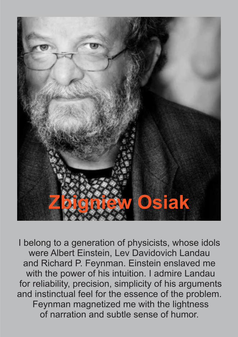
Zbigniew Osiak

I belong to a generation of physicists, whose idolswere Albert Einstein, Lev Davidovich Landau

and Richard P. Feynman. Einstein enslaved mewith the power of his intuition. I admire Landau

for reliability, precision, simplicity of his argumentsand instinctual feel for the essence of the problem.

Feynman magnetized me with the lightnessof narration and subtle sense of humor.