ANT COMMUNITIES OF FLORIDA’S UPLAND ECOSYSTEMS: ECOLOGY AND

SAMPLING

By

JOSHUA R. KING

A DISSERTATION PRESENTED TO THE GRADUATE SCHOOL OF THE UNIVERSITY OF FLORIDA IN PARTIAL FULFILLMENT

OF THE REQUIREMENTS FOR THE DEGREE OF DOCTOR OF PHILOSOPHY

UNIVERSITY OF FLORIDA

2004

Copyright 2004

by

Joshua R. King

To my wife. Thank you for teaching me what is truly important in life.

ACKNOWLEDGMENTS

I would like to thank my committee members John Capinera, Mark Deyrup,

Robert McSorley, Sanford Porter, and Kenneth Portier for reading the dissertation and

providing sound advice on the politics of academia, statistics, publishing, teaching, and

the pursuit of biological knowledge. Their contributions have all aided in my

development as a scientist, collaborator, and colleague; for that I am grateful. In

particular I would like to thank my advisor, Sanford Porter. None of this work could

have been accomplished without the support, laboratory space, equipment, and

encouragement he provided.

I am grateful to Lloyd Davis for teaching me to be a better collector and observer

of the natural world. A man who has forgotten more entomology than I will ever know,

he has impressed on me that a broad entomological knowledge is the best context within

which to build an understanding of ants. I am indebted to Mark Deyrup for showing me

that it is possible to know how to identify everything, and that I must not forget that

sampling and theory can never replace collecting and natural history. Thanks go to Lloyd

Morrison for sharing ideas, insight on being a better scientist, surfing, and Frisbee. I

thank Sanford Porter and Walter Tschinkel for sharing ideas and showing me the

importance of a mechanistic, experimental approach to studying ants. I also thank Walter

Tschinkel and his lab group for sharing ideas and being patient while I finished.

I thank Lloyd Davis and Mark Deyrup for assisting with and verifying species

identifications. I am also grateful for myrmecological advice from Stefan Cover, without

iv

which the project would not have been as successful. I thank the Archbold Biological

Station and Mark Deyrup for laboratory space and accommodation during part of this

work. I thank the University of Florida, the Florida Department of Environmental

Protection’s State Parks Division, and the U.S. National Forest Service for permission to

perform sampling in the Katherine Ordway Biological Preserve, San Felasco Hammock

State Park, and Osceola National Forest, respectively. Voucher specimens from this

project have been donated to Harvard’s Museum of Comparative Zoology and the

Archbold Biological Station. I thank the University of Florida for financial support

during part of my graduate studies in the form of a University of Florida Alumni

Fellowship. I also thank Walter Tschinkel for financial support during the completion of

the dissertation.

I sincerely thank my mother, Pamela Snow, for instilling in me a love of

scholarship, the natural world, and writing. I am also indebted to her for teaching me

patience and the desire to always be optimistic and forward-moving, no matter how rough

the going gets or how daunting the task. I am indebted to my wife, Kari, for teaching me

to be more disciplined. I am also grateful to my wife for emotional support and for

sharing her life with me. Without these things I would not have been able to complete

the dissertation. Finally, I thank my daughter Maizie for showing me what a joy life can

be.

v

TABLE OF CONTENTS page ACKNOWLEDGMENTS ................................................................................................. iv

LIST OF TABLES........................................................................................................... viii

LIST OF FIGURES ........................................................................................................... ix

ABSTRACT.........................................................................................................................x

CHAPTER 1 INTRODUCTION ........................................................................................................1

2 ASSEMBLY RULES FOR INSECTS AT LOCAL AND REGIONAL SCALES: ABUNDANCE, DIVERSITY, AND BIOMASS OF ANTS IN FLORIDA’S UPLAND ECOSYTEMS .............................................................................................4

Introduction...................................................................................................................4 Study Area and Methods ..............................................................................................8

Upland Ecosystems ...............................................................................................8 Inventory Design .................................................................................................12 Analysis ...............................................................................................................14

Results.........................................................................................................................22 Species Richness .................................................................................................22 Abundance and Biomass .....................................................................................22 Behavioral Dominance ........................................................................................27 Species Co-occurrence ........................................................................................28 Introduced Species...............................................................................................29

Discussion...................................................................................................................30 Taxocene Attributes.............................................................................................30 Biogeography, Synthesis, and Applications........................................................50

3 EVALUATION OF SAMPLING METHODS AND SPECIES RICHNESS

ESTIMATORS FOR ANTS IN UPLAND ECOSYSTEMS IN FLORIDA..............78

Introduction.................................................................................................................78 Methods ......................................................................................................................83

Study Area ...........................................................................................................83 Sampling..............................................................................................................83

vi

Analysis ...............................................................................................................85 Results.........................................................................................................................90

Observed and Estimated Species Richness .........................................................90 Rarity ...................................................................................................................92 Complementarity of Ecosystems.........................................................................92 Effectiveness of Sampling Methods....................................................................93

Discussion...................................................................................................................95 Inventory Completeness ......................................................................................95 Performance of Species Richness Estimators......................................................97 Rarity ...................................................................................................................98 Efficiency of Sampling Methods.......................................................................100

4 CONCLUSION.........................................................................................................113

LIST OF REFERENCES.................................................................................................116

BIOGRAPHICAL SKETCH ...........................................................................................132

vii

LIST OF TABLES

Table page 2-1 Species list ................................................................................................................59

2-2 Species richness, slope (m), and R2 values for fitted lines .......................................63

2-3 Five most abundant species ......................................................................................64

2-4 Co-occurrence patterns of ants .................................................................................65

2-5 Body size overlap patterns of ants............................................................................66

2-6 Ant species turnover .................................................................................................67

3-1 Species richness estimates and measures of inventory completeness ....................105

3-2 Mean percent faunal complementarity among ecosystems ....................................106

3-3 Percent faunal complementarity of sample methods. .............................................107

viii

LIST OF FIGURES

Figure page 2-1 Map of Florida ..........................................................................................................68

2-2 Rarefaction curves for ecosystems ...........................................................................69

2-3 Relationship between species occurrences and body mass ......................................70

2-4 Relationship between species richness and body mass ............................................71

2-5 Relationship between species richness and species occurrences..............................72

2-6 Rank abundance distributions...................................................................................73

2-7 Abundance and biomass of ants ...............................................................................74

2-8 Abundance, occurrence, and biomass of common species.......................................75

2-9 Baits occupied and occurrences of species...............................................................76

2-10 Native and introduced species richness per ecosystem ............................................77

3-1 Species richness, uniques, and estimated richness .................................................108

3-2 Efficiency of individual and combined sample methods........................................109

3-3 Similarity of ant species as a function of distance..................................................110

3-4 Total time and unique species by different methods ..............................................111

3-5 Relationship between site richness and method richness .......................................112

ix

Abstract of Dissertation Presented to the Graduate School of the University of Florida in Partial Fulfillment of the Requirements for the Degree of Doctor of Philosophy

ANT COMMUNITIES OF FLORIDA’S UPLAND ECOSYSTEMS: ECOLOGY AND

SAMPLING

By

Joshua R. King

December, 2004

Chair: Sanford Porter Major Department: Entomology and Nematology

The empirical relationships among species richness, relative abundance, and body

size in different habitats and at local and regional scales may help to elucidate the factors

responsible for existing patterns of community structure. Accurately measuring these

relationships among invertebrates requires a robust sampling methodology. I used

structured inventory to thoroughly sample ant communities in five upland ecosystems in

north-central Florida using pitfall traps, litter extraction, baits, and hand collecting. I

evaluated the efficiency of a variety of methods for sampling ant species richness and

relative abundance (pitfall traps, litter extraction, baits, and hand collecting). I also

evaluated the performance of four species richness estimators.

A total of 37,961 ants of 94 species were captured, identified, and weighed to

determine biomass. Results showed that Florida’s ground-dwelling ant communities (1)

are numerically dominated by a few, common, generalist southeastern and eastern

species; (2) exhibit a unimodal relationship among species richness, number of species

x

occurrences, and body mass of workers; (3) have the greatest proportion of biomass of

foraging workers among a few species with the largest individual workers; (4) have

random species co-occurrence patterns and nonrandom patterns of size variance across

ecosystems; and (5) are apparently not strongly impacted by introduced species in

relatively undisturbed native ecosystems.

Sampling captured ~66% of the regional fauna and ~70 to 90% of species within

the ecosystems studied. For sampling species richness, combinations of sampling

methods were much more effective than individual methods. Nonparametric estimators

performed better than lognormal fitting, or Michaelis-Menten curve extrapolation.

However, none of the estimators were stable and their estimates should be viewed with

trepidation.

A general rule of resource division (e.g., overlapping niches), together with similar

minimum populations sizes adequately determines the relationship between species

richness and abundance. The way that the impact of introduced ant species is assessed is

evaluated and alternative assessments are proposed. The Ants of the Leaf Litter (ALL)

protocol is recommended for thoroughly sampling ant assemblages in temperate and

subtropical ecosystems.

xi

CHAPTER 1 INTRODUCTION

There is evidence that, at continental and regional scales, patterns of ant diversity

conform to the energy limitation hypothesis (sensu Rosenzweig and Abramsky 1993)

across temperate and tropical regions (Kaspari et al. 2000a, b). At continental scales, net

primary productivity (NPP), mean monthly temperature, and seasonality have been

shown to account for variation in ant abundance (Kaspari 2001). This evidence has

important implications for exploring how environmental conditions determine the

distribution, abundance, and diversity of ants, insects, and ectotherms in general at a

variety of scales. In spite of this evidence, and the obvious importance of these

organisms in ecosystem function and the maintenance of global biodiversity, there are

surprisingly few comprehensive studies documenting their abundance, biomass, and

diversity in relation to environmental change at a variety of scales.

Habitat modification, exotic species invasions, and climatic shifts are threats to

insect biodiversity at all scales. Yet understanding the depth and breadth of impacts or

predicting the eventual outcome of these phenomena remains a largely conjectural

endeavor. We know little about distribution, abundance, and species richness patterns for

many insects and we know less about the mechanisms underlying the patterns. Much of

the problem is a result of ineffective sampling methods and/or undersampling (Longino

and Colwell 1997, Fisher 1999a). It is practical (and logical) to integrate the examination

of patterns of biodiversity and community structure of natural communities with an

assessment of sampling methods.

1

2

Among insects, ants are unique because of their ubiquity, abundance, and

importance in ecosystem functioning in nearly every terrestrial environment. Ants and

other social insects, such as termites, often account for the majority of animal biomass in

ecosystems (Hölldobler and Wilson 1990). As such, ants deserve consideration as a

keystone taxon for their role in the flow of energy through ecosystems. Ants are among

the principal animal motivators for ecosystem processes such as nutrient cycling, soil

turnover, and aeration (Hölldobler and Wilson 1990). Additionally, in most ecosystems

they are the primary predators and scavengers of insects, and in some ecosystems they

are the principle herbivores and granivores (Davidson et al. 2003). Finally, there is

evidence that ants may play a central role in the dispersal and success of numerous plant

species (Hölldobler and Wilson 1990).

For most ant species, colony founding (a colonization event) is claustral. This

means that a single, reproductive female, after mating, finds a suitable nesting site, seals

herself in and rears her first generation of workers from her own energy reserves. While

a vast majority of queens are killed prior to establishing a nest chamber (by predators or

desiccation), success for those that do manage to survive then becomes dependent on

suitable environmental conditions for brood development. Through time, natural

selection will strongly favor foundresses that select sites with conditions that allow

maximum energy harvest with minimal metabolic costs (Kaspari et al. 2000b). For ants

(ectotherms), this process supposes a balancing act where, over time, those species that

best exploit the relationship between temperature and metabolic costs in a given

ecological niche will be more productive and dominate that niche. At larger scales,

regions that support conditions better suited to the maximization of the temperature-

3

metabolic cost relationship will support a greater abundance of ants (Kaspari et al.

2000b). The majority of ant species are thermophilic and low temperature is the primary

abiotic stress affecting community structure (Andersen 1995). In this context it is

realistic to test hypotheses that ant assemblages are structured by a dynamic interaction of

these factors at smaller scales.

The increasing frequency of introductions and associated economic costs of exotic

ants in North America and throughout the world warrants a closer examination of their

distribution and abundance at local and regional scales and in a variety of habitats.

Exotic ants are becoming more widespread and are often correlated with reductions in the

biodiversity of insects, small vertebrates, and plants, and with negative impacts on human

society (Holway et al. 2002). Among the 147 known exotic ants recorded outside of their

native regions (McGlynn 1999), Solenopsis invicta, commonly referred to as the red

imported fire ant, is of particular interest due to its common negative interaction with

humans (Lofgren 1986, Vinson 1994), our inability to slow its spread in the U.S., and its

range expansion into the Caribbean, New Zealand, and Australia.

The ant fauna of Florida includes 218 species, 52 of which are classified as exotic

(Deyrup 2003). The regional distribution of most species is well known and has been

studied for decades (Deyrup 2003). Within the state, highly disturbed areas (e.g.

agricultural and urban landscapes) are dominated by invasive, exotic species (particularly

S. invicta, Deyrup et al. 2000). Much less is known about the species richness, relative

abundance, and biomass of native and exotic ant species in upland habitats and the

mechanisms that may determine these patterns. For these reasons, Florida provided the

ideal setting for investigating these relationships.

CHAPTER 2 ASSEMBLY RULES FOR INSECTS AT LOCAL AND REGIONAL SCALES:

ABUNDANCE, DIVERSITY, AND BIOMASS OF ANTS IN FLORIDA’S UPLAND ECOSYTEMS

Introduction

Insects represent one of the most functionally important and the most diverse taxon

among terrestrial animals. Improving our understanding of insect community ecology

would contribute significantly to a better comprehension of patterns of terrestrial

biodiversity and the processes which generate it (Wilson 1987). Determining the factors

responsible for these patterns requires information on how individual insects interact with

their environment (abiotic and biotic). The body size (biomass) of an individual is

correlated with metabolism, reproductive rate, and diet, among many other biologically

important characteristics (Peters 1983, Calder 1984). Body size, species richness, and

relative abundance are also interdependent (Peters 1983, Morse et al. 1988, Siemann et

al. 1996). Thus, body size provides a link between the biology of individual organisms

and the ecology of populations and ecosystems (Calder 1984, Brown et al. 2004).

Species richness is a function of immigration and extinction (MacArthur and

Wilson 1967). The rates of immigration and extinction are dependent on abundance and

body size (Pimm et al. 1988, Ricklefs and Schluter 1993, Siemann et al. 1996, 1999).

Species interactions (e.g., competition) occur most frequently among species similar in

size and ecology (Brown and Wilson 1956). Body size variation is limited by phylogeny

(Maurer et al. 1992, Brown et al. 1993). Consequently, species richness should be at

least partly dependent on the number of individuals within a group of interacting, related

4

5

species (Kaspari et al. 2003), although the nature of this relationship may vary across

taxonomic levels (e.g., class, order, family, genus) (Siemann et al. 1996, 1999, Kaspari

2001).

Over time, the selective force of species interactions can result in adaptive shift

(e.g., character displacement), which also contributes to local and regional diversity

(Brown and Wilson 1956). Examining relationships among body size, species richness,

and relative abundance within monophyletic assemblages of interacting taxa within a

given area (taxocenes, Hutchinson 1978) is therefore, of particular interest. Many

previous studies have focused on higher taxonomic levels (i.e., class, order) (Janzen

1973, Morse et al. 1988, Bassett and Kitching 1991, Stork and Blackburn 1993, Siemann

et al. 1996, 1999). However, examining these relationships across lower taxonomic

levels (i.e., family, genus, species) may more clearly reveal how factors such as abiotic

conditions, trophic biology, biogeographic history, and interspecific competition have

determined ecological and evolutionary diversification at local and regional scales (Lack

1947, Brown et al. 1993, Ricklefs and Schluter 1993). For observational studies (natural

experiments), examining monophyletic lineages reduces some of the ecological and

evolutionary variability found within species assemblages. This approach facilitates the

derivation of general rules (if they exist) that govern the way species assemblages come

together. These assembly rules are a product of species interacting with each other and

with their environment, and culminate in the extinction and evolution of species

(Diamond 1975, Brown and Maurer 1987, Gotelli and McCabe 2002). Assembly rules

that are consistent across a wide range of taxonomic levels (from species to class) and

6

body sizes may indicate what the most important factors determining patterns of body

size, species richness, and abundance within natural communities.

Among insects, ants (Hymenoptera: Formicidae) are an important group for

ecological study. Ants are nearly ubiquitous, functionally important, speciose, and

among the most abundant organisms in tropical, subtropical, and some temperate

terrestrial ecosystems (Hölldobler and Wilson 1990, Tobin 1994, Wilson 2003). They

exert significant influence on the biotic and abiotic features of the ecosystems they

occupy, and are among the most studied terrestrial invertebrate taxa (Hölldobler and

Wilson 1990, Folgarait 1998). Sampling techniques are well established (Agosti et al.

2000a). Specimens can be identified to the species level for most North American

species, particularly in Florida (Creighton 1950, Deyrup 2003). The structure of ant

assemblages has been shown to change predictably in response to shifts in vegetation and

soil (Majer 1983, Andersen 1991, Bestelmeyer and Wiens 1996, King et al. 1998).

Accordingly, ants have been used to monitor the environmental impacts of large-scale,

anthropogenic disturbance and subsequent ecosystem recovery (Andersen 1990, 1993).

Additionally, introduced ant species are widely distributed and warrant monitoring

because some have been documented to impact native faunas, ecosystems, and human

societies where they occur (Adams 1986, Lofgren 1986, McGlynn 1999, Holway et al.

2002).

Studies of ant assemblages using diverse methods and extensive sampling to

examine ecological patterns showed that species richness, abundance, and body size

reflect assembly rules determined at least partly by interspecific competition,

temperature, and energy availability (productivity) at regional and geographic scales

7

(Kaspari et al. 2000a, b, 2003, 2004, Kaspari 2001, Gotelli and Ellison 2002a, b). For ant

assemblages, intra- and interspecific competition at small scales has been the most

studied form of species interactions (Davidson 1977, Vepsäläinen and Pisarski 1982,

Morrison 2000) and is widely assumed to be the most important factor in determining

assembly rules (Hölldobler and Wilson 1990). Temperature, moisture, and ground cover

have also been used to explain structure in assemblages from local to continental scales

(Levings and Windsor 1984, Andersen 1995, 1997b, Morrison 1998, Kaspari et al.

2000b). For ants (and insects in general), species interactions, body size, biogeographical

history, and trophic biology are also important in determining assembly rules. Ant

assemblages (like all taxocenes) have numerous, measurable characteristics or ‘axes’

along which taxon attributes can be ordinated and used to determine their role in

determining assembly rules (Whittaker 1975). Characteristics include species richness,

relative abundance, body size, species turnover, behavioral dominance, total biomass,

spatiotemporal distribution, and trophic biology (Colwell and Coddington 1994, Krebs

1994). These characteristics can be quantified by sampling and are, accordingly, subject

to the bias of individual sampling methods (Bestelmeyer et al. 2000).

A large sampling effort and the use of a variety of methods is the most effective

approach to sampling ants at local scales, and permits separation of sampling effects from

ecological effects (Longino and Colwell 1997). Reduced sampling efforts limit the scope

of the study to a small subset of the fauna (Longino and Colwell 1997), which may or

may not actually be interacting. Such results cannot be said to be representative of

patterns within entire assemblages (Chapter 3). A more comprehensive approach to

8

sampling and analyzing structure in ant assemblages is required to reveal the underlying

factors responsible for assembly rules at local and regional scales.

Here I report a study of the ants of the upland habitats of Florida at local and

regional scales. My work represents one of the most comprehensive ecological studies of

a regional ant fauna. I used an intensive sampling design to generate data for a

comprehensive analysis of structure within ant assemblages. In so doing, I sought to

determine the general assembly rules of the ants of this region. I measured species

richness, relative abundance, monopolization of baits, relative biomass of foraging

workers, species co-occurrence patterns, size ratios of species, and species turnover

among ecosystems. I also determined the distribution and abundance of introduced ant

species in native ecosystems. Florida has the highest number of introduced ant species in

North America, and the impact of these species on native fauna is poorly understood

(Deyrup et al. 2000). Finally, I evaluated results in the context of current conservation

and pest management priorities relevant to ants in native upland ecosystems in Florida.

Study Area and Methods

Upland Ecosystems

Florida is ecologically unique because its geographic features create a productive

and humid environment anomalous to a latitudinal range globally characterized by

deserts (Myers and Ewel 1990a). Of particular interest is the high level of endemism

among native plants and animals, despite the low relief of the region (Hubbell 1960) and

its broad connection to southeastern North America. Upland ecosystems in north-central

Florida are representative of native terrestrial ecosystems elsewhere in the southeastern

coastal plain, and also include ecosystems unique to the state (Myers and Ewel 1990a).

These ecosystems represent a productivity gradient ranging from closed canopy

9

hardwood forests to completely open herbaceous savannah. Historically, peninsular and

continental upland ecosystems were probably distributed as a mosaic of different plant

communities determined by geographic factors such as soil types and water-drainage

patterns, modified by natural disturbance events such as fire and hurricanes (Webb 1990).

Many of these plant communities now occur as more or less isolated patches of various

sizes, surrounded by a matrix of roads and agricultural and urban development (Myers

and Ewel 1990b). Anthropogenic disturbance in the form of road building, fire

suppression, logging, and introduced species invasions have impacted almost all of the

remaining upland ecosystems to some degree.

Ants were surveyed in four localities in north and central Florida on the inland

region stretching from Columbia County in the north, south into Highlands County along

the Lake Wales Ridge (Fig. 2-1). Using the ecosystem criteria of Myers and Ewel

(1990a), I sampled in the four most common, widespread natural upland ecosystem types

in Florida: (1) temperate hardwood forests at the San Felasco Hammock State Park, (2)

pine flatwoods at the Osceola National Forest, (3) high pine at the Katherine Ordway

Biological Preserve, and (4) Florida scrub at the Archbold Biological Station. I also

included a fifth category of a disturbed ecosystem, consisting of cleared field habitats.

The localities were selected as representative of some of the least-disturbed remaining

native upland ecosystems in peninsular Florida. Localites were selected that contained

sufficient contiguous, relatively homogeneous areas of each plant community to

accommodate three, large (180 m) linear transects separated by at least 100 m from roads,

fences, or edges (e.g., park boundaries or ecotones). Within localities, transects were

separated by at least 1 km with the exception of two transects in San Felasco Hammock

10

State park that were within 200 m of each other. The principal purpose of the sampling

design was to produce a relatively complete species list and associated abundance data

for a representative example of each upland ecosystem in the region, and of the region as

a whole. When possible, localities were chosen where previous, thorough ant inventories

had been performed (e.g., Deyrup and Trager 1986), to facilitate an evaluation of

inventory completeness (Chapter 3).

Hardwood hammock. Temperate hardwood forests, frequently called hammocks,

are not extensive in Florida. Hammocks are often associated with mesic, sandy,

organically rich soils in riparian zones, and with the regions between high pine forests

and wet prairies (Platt and Schwartz 1990). Hammocks in north Florida contain the

largest numbers of tree and shrub species per unit area in the continental U.S., and have

an extremely diverse overstory and understory structure relative to other temperate

forests (Platt and Schwartz 1990). Structurally, these forests typically have a closed

canopy, a diverse understory, and a deep layer of leaf litter.

Pine flatwoods. Throughout recent history, the most common and widespread

upland habitat in Florida has been pine flatwoods. These forests are associated with flat

topography, and poorly drained, acidic, sandy soil (Laessle 1942, Abrahamson and

Hartnett 1990). They are structurally characterized by an open overstory of pines (Pinus

palustris Mill. and P. elliottii Engelm.) and a dense understory layer [the dominant

species include Serenoa repens (W. Bartram) Small, Ilex glabra (L.) A. Gray, Lyonia

lucida (Lam.) K. Koch, Aristida beyrichiana Trin. & Rupr., and other herbs] (Laessle

1942, Abrahamson and Hartnett 1990).

11

High pine. High pine are savannah-like ecosystems occurring on rolling

topography and well-drained, sandy soil (Abrahamson et al. 1984, Myers 1990). Tree

species composition is a mixture of pine (P. palustris, P. elliottii) and oak (particularly

turkey oak, Quercus laevis Walter) (Abrahamson et al. 1984, Myers 1990). The structure

of high pine communities is characterized by an open canopy of pine and hardwoods, an

open understory of mixed hardwood species, and a sparse-to-dense herbaceous ground

cover (A. beyrichiana) (Abrahamson et al. 1984, Myers 1990). A small number of

species endemic to Florida and the southeastern coastal plain are associated with high

pine (Myers 1990).

Florida scrub. In the eastern U.S., Florida scrub forests (henceforth, scrub)

ecosystems occur almost exclusively in Florida and are structurally characterized by a

sparse overstory of pines, a dense understory of stunted hardwoods and shrubs, and very

sparse herbaceous ground cover (Myers 1990). These densely vegetated, stunted forest

ecosystems are associated with xeric conditions and well-drained, sandy soil

(Abrahamson et al. 1984). The most common species of pine are P. clausa or P. elliottii.

The shrub understory is dominated by xerophytic oaks (e.g., Q. geminata Small, Q.

myrtifolia Willd., and Q. chapmanii Sarg.), shrubs [e.g., L. ferruginea (Walter)], or

rosemary (Ceratiola ericoides Michx.) (Abrahamson et al. 1984). Most of Florida’s

endemic plant and animal species in upland ecosystems are associated with scrub

ecosystems (Myers 1990).

Fields. For the purposes of my study, previously cleared (> 20 years ago),

ungrazed fields were chosen to represent disturbed conditions. These ecosystems can be

found throughout the central inland ridges of north and central Florida, and were chosen

12

because they are a major component of land acquisition and rehabilitation projects in the

state (Jue et al. 2001). Structurally, fields are characterized by an absence of trees and a

moderate to dense herbaceous ground cover. Floristically, the fields sampled were

composed primarily of introduced grass species, native grasses, and a few, scattered

shrubs.

Caveats. The primary limitation on locality selection was that, with the exception

of field habitats, ecosystem types could not be replicated in each locality. These

limitations are imposed by the current distribution of relatively undisturbed native upland

ecosystems in Florida. Sites were replicated within ecosystems at each locality. But, the

historical biogeography of upland ecosystems of the central inland ridge of the peninsula

is different from ecosystems along the eastern and western coasts, south Florida, the

panhandle, and the southeastern coastal plain (Myers and Ewel 1990a). Consequently,

some species assemblage characteristics will vary within the same type of ecosystem in

different localities throughout the region (e.g., the species composition of pine

flatwoods). Nevertheless, the relative differences in assemblage characteristics (e.g.

species richness and abundance) I report among ecosystems are consistent with ant

surveys (Van Pelt 1956, 1958, Deyrup and Trager 1986, Lubertazzi and Tschinkel 2003)

previously conducted elsewhere in the region.

Inventory Design

Sampling was performed from June to September 2001. This sampling period was

chosen because it typically includes the warmest and wettest months of the year, and thus

is the period of maximum ant activity in Florida. Seasonal variability of ant assemblages

was not addressed. Sampling was performed at least 72 h after (and never included)

rainfall events to minimize the impact of higher ant activity immediately following

13

rainfall during warm months (J.R. King pers. obs.). Four methods were used to capture

ground-dwelling ants: baiting, pitfall trapping, leaf litter extraction with Berlese funnels,

and standardized hand collecting.

Three study sites were chosen within each of the five selected ecosystems for a

total of fifteen study sites. Within each site, a starting point was selected, and a transect

was laid out in a randomly chosen direction. Transects consisted of 3 separate sampling

lines. One line of 36 pitfall traps and one line of 36 litter samples were first placed

parallel to one another and separated by 10 m (Fisher 1996, 1998, 1999b, 2002). Along

each line samples were placed at 5 m intervals (180 m total). The third line of 36 baits

was placed between the pitfall and litter extraction lines, with baits placed every 5 m,

corresponding to the placement of each pitfall and litter extraction sample. The bait

transect was placed (and the baits operated) after pitfall and litter samples had been taken.

Pitfall traps were 85-mm-long plastic vials with 30 mm internal diameter. Traps

were filled to a depth of approximately 15 mm with propylene-glycol antifreeze, and

operated for 3 days. Litter samples were taken immediately after setting pitfall traps.

Each sample was obtained by collecting all surface material and the first ~ 1 cm of soil

within two 0.25 m2 quadrats. The two samples were pooled; larger objects (e.g., logs)

were macerated with a machete, and the pooled samples were sifted through a sieve with

1 cm grid size. Sifted litter was placed in covered metal 32-cm-diameter Berlese funnels,

under 40 watt light bulbs. The funnels were operated until the samples were dry (~ 48 to

72 h). Baits were 12 × 75 mm test tubes with a piece (2 g) of hot dog (Oscar Mayer®

beef franks, Northfield, Illinois) inserted ~ 2 cm into the tube. At each sampling point, a

small spot was cleared of any litter and the bait tube was placed directly on the ground (to

14

speed discovery and access), and shaded with one half of a Styrofoam plate. The baits

were operated for 0.5 h, collected, and the ends plugged with small cotton balls to prevent

the ants from escaping. Throughout the operation of baits, brief observations of the

behavior of ants were made at haphazardly selected baits. Hand collecting consisted of

searching vegetation, logs, and leaf litter, and breaking open twigs for 2 h in the

immediate vicinity of each site.

Analysis

The inventory design permitted the analysis of assemblages at local (three replicate

transects within each ecosystem) and regional (all data combined) scales. For all

analyses, only records for worker ants were included, as the presence of queens or males

in samples is not necessarily indicative of an established colony (Fisher 1999a).

Specimens were sorted and species were identified by J.R. King. Species that could not

be definitively identified by workers alone (e.g., separating some species requires

associated queens) were identified as “near” (sp. nr.) the most similar species description.

The relative productivity (net aboveground productivity) of ecosystems was

estimated from studies of hardwood hammock (Lugo et al. 1978, Megonigal et al. 1997),

pine flatwoods (Golkin and Ewel 1984, Gholz et al. 1991), high pine (Mitchell et al.

1999), scrub (Schmalzer and Hinkle 1996, Schortemeyer et al. 2000), and old field

(Odum 1960) conducted in Florida or the southeastern United States. Among the

localities studied here, the relative differences in net aboveground productivity among

ecosystems are primarily a result of differences in soil characteristics (e.g., moisture

retention, nutrient availability), and not of differences in latitude and rainfall (i.e.,

insolation, temperature, and annual precipitation differ little among localities, J.R. King

unpublished data). Using these data as an estimate for net aboveground productivity in

15

each of the ecosystems sampled in this study, a gradient of relative productivity was

approximated where hardwood hammock (~ 1500 g.m-2.yr-1) > pine flatwoods (~ 900

g.m-2.yr-1) > scrub (~ 500 g.m-2.yr-1) > high pine (~ 400 g.m-2.yr-1) > field (~ 300 g.m-2.yr-

1).

Species richness. Species richness was examined within ecosystems using

rarefaction curves generated by random re-orderings (50 times) of samples using the

program EstimateS (Colwell 2000). To compare richness between ecosystems, curves

were generated from pooled data that included all methods used at each site. For

comparisons among ecosystems, samples from all methods at each of the three replicate

sites per ecosystem were pooled. I compared sample-based rarefaction curves with the

observed number of species plotted on the ordinate against species occurrences

(presence/absence data) plotted on the abscissa, to assess differences in species richness

between and among curves representing sites and ecosystems (Colwell and Coddington

1994, Gotelli and Colwell 2001). Species occurrences (rather than numbers of

individuals) were used to examine species richness because ants are social and therefore

spatially clumped. This problem is exacerbated by sampling techniques that aggregate

individuals (baits) or capture entire colonies (litter samples). Additionally, hand

collecting is only useful for producing presence/absence records (Bestelmeyer et al.

2000). Species density (the total number of species captured per unit area, Gotelli and

Colwell 2001) was also compared across ecosystems.

Abundance and biomass. I used two measures to assess abundance per species:

the total number of individuals, and the number of occurrences in both pitfall and litter

samples. The number of individuals provides an estimate of the numerical abundance of

16

foraging workers and cumulative biomass (a multiple of species abundance). Species

occurrences provide a measure of spatial abundance (i.e., the number of times a species

occurs per unit area). Analyses based on species occurrences also permits comparisons

among datasets generated with different sampling methods. For ants (and other social

insects), using multiple sampling techniques to evaluate species occurrences, numerical

abundance, and biomass of foraging workers provides clearer resolution of the different

dimensions of ant species abundance.

Abundance of individual workers and total worker biomass for pitfall and litter

samples were totaled for each site, and then averaged within ecosystems. Relative

abundance and relative biomass of each species were also calculated within ecosystems.

Only the 76 ground-dwelling species sampled by pitfall or litter extraction were included

in this part of the analysis, as arboreal species were not adequately sampled by methods

used. As subterranean fauna were generally well-represented in pitfall and litter

sampling (values were compared with relative abundance in subterranean baits, J.R. King

unpublished data), they were included in analyses.

Total foraging worker biomass was computed by multiplying the abundance of

workers by their average dry mass (mg). The dry mass values of workers should be

considered approximations as they do not account for variation (e.g., changes in seasonal

fat content, worker polymorphism) within species. For Pheidole species I used only the

mass of minor workers as majors were uncommon in samples. There were 23 species for

which weights were not taken because they were mounted as vouchers. For these

species, the biomass of a similarly sized species in the same genus was rounded to the

nearest fraction (tenth, hundredth, thousandth) of a milligram and used as an

17

approximation. The direction and magnitude of rounding was determined by taking

relative body size measurements using Weber’s length (Brown 1953). This approach

provides an approximation of unknown biomass similar to other approaches (e.g.,

regressive body length/biomass relationships, Rogers et al. 1976, Kaspari and Weiser

1999). A majority of species without measured weights were rare (appearing in < 1% of

samples) and had little impact on total biomass estimates. The rounded values were also

applied in the assignment of species size categories and the size ratio analysis.

To facilitate comparisons of ant assemblages with entire insect communities, I

generally followed Siemann and colleagues’ (1999) approach to analyzing relationships

among abundance, body size, and species richness at local (ecosystem) and regional (all

data combined) scales. Species occurrences were pooled within ecosystems. To evaluate

relationships among species richness, body size, and abundance at local and regional

scales, species number, species occurrences, and individual abundances were log10

transformed and summed within log2 individual worker biomass classes. My analyses of

body size, abundance, and species richness within and among ecosystems required only

that measures of abundance and species richness be relative (Maurer and Brown 1988,

Siemann et al. 1996, 1999), although the completeness of the inventory suggests that

these measures are relatively accurate as well (Chapter 3). These values were then

plotted against the number of species occurrences and the number of species. A

modified, nonparametric smoothing procedure was used to fit regressions through these

points to validate the use of the arbitrarily selected log2 size class intervals (Maurer and

Brown 1988, Siemann et al. 1999). The method fits a curve to the relationship between

the number of species or the number of species occurrences and biomass by summing

18

them within a fixed width interval (1.0 unit in log2 scale) that is moved in increments (0.1

in log2 scale) through the entire range of body sizes (Maurer and Brown 1988, Siemann

1999).

Ordinary least-squares regressions were used on log10 (henceforth, log) transformed

data to test the dependence of species richness on the number of species occurrences and

on the total biomass (abundance × mean worker biomass) summed within log2 body mass

classes at local and regional scales. At the regional scale, species occurrence data were

ranked and plotted as log species occurrence versus log rank within log2 body mass

classes. This distribution was then visually compared with geometric, lognormal, and

broken-stick distributions. All regressions were ordinary least-squares regressions.

Throughout, significance is assessed at the P ≤ 0.05 level.

Behavioral dominance. Behavioral dominance at baits was used in combination

with combined pitfall and litter sample occurrences to compare spatial occurrence with

behavioral dominance. Dominance was determined by the percentage of baits occupied

per species. Percent of baits occupied was then plotted with the percent occurrence in

pitfall and litter samples for all species to compare patterns of behavioral and spatial

dominance. Only species appearing in baits were used in this analysis. For some

ecosystems the total percentage of baits occupied by all species exceeded 100% due to

occasional co-occurrence of species at baits.

Species co-occurrence. Species co-occurrence patterns were examined to test

whether upland Florida ant communities are non-random assemblages (against a null

hypothesis that they are randomly assembled) following Gotelli and Ellison’s (2002b)

analytical approach. I used combined occurrence data from pitfalls and litter samples for

19

each transect for all analyses (for all analyses using either pitfall or litter sample data

separately produced nearly identical results). I analyzed co-occurrence patterns at both

the local (ecosystem) and regional (all sites combined) scales. Only ground-dwelling

species sampled by pitfall or litter extraction were included in these analyses (a regional

source pool of 76 species). The regional-scale data were organized as a species (rows, n

= 76) by sites (columns, n = 15) presence-absence matrix. The local scale data were

organized as a species (rows) by sample (combined pitfall and litter sample, n = 36)

presence-absence matrix. C-scores (Stone and Roberts 1990) were calculated as a metric

for co-occurrence within the matrices. Larger C-scores indicate fewer pairwise species

co-occurrences and a competitively structured assemblage should have scores greater

than expected by chance (Gotelli and Entsminger 2001). I compared the observed C-

score to a histogram of 10,000 C-scores that were generated from randomly constructed

null assemblages and determined the exact tail probability for the observed value based

on the null model histogram (Gotelli and Ellison 2002b). I analyzed each site occurrence

matrix using three null models that use row and column constraints to test a variety of

ecological scenarios: fixed-fixed, fixed-equiprobable, and weighted-fixed (detailed in

Gotelli and Ellison 2002b). In the fixed-fixed null model the row and column sums are

preserved in the null community so that the number of species and species occurrences

are the same as the observed community. In the fixed-equiprobable null model only the

row sums are fixed and the columns (= sample points) are equiprobable. In the weighted-

fixed null model the column totals are fixed but the frequency of each species is

proportional to the total number of occurrences in pitfall and litter samples within a site.

As the fixed-equiprobable model treats all sites as equiprobable (a biologically unrealistic

20

assumption at the regional scale where sites are different ecosystems), I analyzed the

regional scale matrix using only the fixed-fixed and weighted-fixed models.

To test that body size ratios showed constant ratios I plotted mean worker ant

biomass on a log scale and calculated the difference between adjacent species. I then

calculated the variance in these segment lengths ( , sensu Gotelli and Ellison 2002b) as

an index of constancy in body size ratios. The observed segment lengths were compared

to a histogram of 5,000 segment lengths that were generated from randomly constructed

null assemblages and determined the exact tail probability for the observed value based

on the null model histogram (Gotelli and Ellison 2002b). A low value of relative to a

randomly assembled community is indicative of competitive structuring. I used four null

models to evaluate size ratios within sites: uniform, equiprobable source pool,

occurrence-weighted source pool, and abundance weighted source pool (detailed in

Gotelli and Ellison 2002b). The uniform null model uses the largest and smallest species

in the assemblage to fix the endpoints of the distribution; the remainder (n -2) species are

chosen from a random, (log) uniform distribution within those limits. In the equiprobable

source pool null model species are drawn randomly and equiprobably from the list of

species compiled for the ecosystem. Once a species is drawn it cannot be drawn again.

This model constrains possible body sizes at the local scale to the range of body sizes

from the ecosystem as a whole. In the occurrence-weighted source pool null model

species are also randomly drawn from the ecosystem species list, however, the relative

probability a species is drawn is proportional to the number of sites (n = 3) in which it

occurred. The abundance-weighted source pool is identical to the occurrence-weighted

null model except the relative probabilities are calculated using the total number of

2slσ

2slσ

21

occurrences in combined pitfall and litter extraction samples in ecosystems. I used only

the uniform model at the regional scale. Species co-occurrence patterns and size ratios

were examined using the program Ecosim (Gotelli and Entsminger 2001).

Species turnover (beta diversity) and the number of shared species were calculated

on a per ecosystem basis to examine the pairwise differences in the amount of species

turnover among ecosystems. Species turnover was assessed using Harrison and

colleagues’ (1992) beta-2, a measure of the amount by which regional species richness

exceeds the maximum species richness attained locally; beta-2 = (S/amax) – 1, where S =

the total number of species sampled from all sites, amax = maximum value of alpha-

diversity. For the purpose of my study I calculated beta-2 by grouping sites by

ecosystem to calculate all pairwise turnover values among ecosystems.

Introduced species. The relationship among introduced ant species, native ants,

and non-ant arthropods was assessed across ecosystems. Species richness of native and

introduced ant species was determined from all sampling methods and analyses of ant

abundances used only data from pitfall and litter extraction samples. Non-ant arthropods

from pitfall and litter extraction samples were identified to morpho-species within

families on a per sample basis (i.e., morpho-species were not compared among samples)

– a highly conservative estimate of species richness per sample point. This was done to

generate a relative sample-point estimate of non-ant arthropod species richness which

could be averaged within sites and compared across ecosystems (Porter and Savignano

1990).

22

Results

Species Richness

Structured, quantitative inventory methods captured 37,961 individual ants

representing 94 species from 31 genera (Table 2-1). The richest genera sampled were

Solenopsis (10 species), Pheidole (7 species), Camponotus (6 species), Paratrechina (6

species), and Pyramica (6 species). Three narrowly endemic species (Dorymyrmex

elegans, Paratrechina phantasma, Pheidole adrianoi) were sampled in high pine and

scrub (Table 2-1). These species are typically associated with deep sandy ridges along

the central peninsula of Florida. Twelve species were arboreal and 9 were subterranean.

Species density was significantly different among ecosystems (ANOVA: F = 4.93,

df = 1,4, P = 0.02) with transects in high pine sites having, on average, the most species

(35 ± 7; mean ± 1 sd) followed by scrub (29 ± 3), pine flatwoods (27 ± 6), hammock (21

± 4), and field sites (20 ± 4), respectively. Sample-based rarefaction curves for pooled

ecosystem data showed that sampling in high pine ecosystems captured the most species

while sampling in hammock sites captured the fewest species (Fig. 2-2). The shape of

the curves also revealed that sampling in high pine sites accumulated species much more

quickly than in the other ecosystems, while species accumulated most slowly in

hardwood hammock. Sampling in scrub and pine flatwoods produced similar numbers of

species and similarly shaped rarefaction curves. The field rarefaction curve approached

an asymptote much more quickly than the other curves.

Abundance and Biomass

The smallest species included Brachymyrmex sp. nov., B. depilis, and the two

smallest Solenopsis (Diplorhoptrum) species, S. tennesseensis and S. tonsa (Table 2-1).

The largest species were Camponotus castaneus and C. socius. At the regional scale, the

23

relationships among individual worker biomass, species occurrences, and number of

species revealed that small to intermediate sized species were most abundant (Fig. 2-3)

and speciose (Fig. 2-4). A similar pattern was seen across all ecosystems. Among

intermediate biomass classes, the most abundant (occurrences and numerical abundance)

species were from the genera Pheidole, Solenopsis (Diplorhoptrum), and Paratrechina,

respectively. The most abundant, large species were Odontomachus brunneus and C.

floridanus.

At the regional scale (all data combined) and among all ecosystems, the

relationship between species richness and body mass was unimodal (sensu stricto), as

was the relationship between abundance and body mass, although there was a distinct

second “hump” that included species with the largest workers. With each species plotted

separately (Fig. 2-3, small filled circles), the log of species occurrences was unrelated to

the log of biomass at the regional scale and among all ecosystems when fitted with linear,

polynomial, or power functions (R2 < 0.01 for all models).

At the regional scale, log transformed species richness (Si) was related to the

number of species occurrences (Oi) as a linear function Si = 0.39Oi – 0.05 (R2 = 0.75, P <

0.01), where i = log2 body mass classes (Fig. 2-5). This relationship is, therefore,

represented by the power function Si = 0.89Oi0.39 for untransformed data. The pattern

was only slightly different among ecosystems (Fig. 2-5), as the linear relationship for

hardwood hammock (Si = 0.65Oi0.36, R2 = 0.82, P < 0.01), pine flatwoods (Si = 1.0Oi

0.32,

R2 = 0.60, P = 0.01), and scrub (Si = 1.01Oi0.32, R2 = 0.57, P = 0.02) exhibited shallower

slopes. In contrast, the linear relationship in field (Si = 0.81Oi0.42, R2 = 0.81, P < 0.01)

and high pine (Si = 0.66Oi0.5, R2 = 0.63, P = 0.01) ecosystems exhibited steeper slopes. In

24

sum, these results indicate a relatively consistent, significant, relationship between

abundance and species richness.

In a multiple regression, the log of species richness (Si) was significantly positively

correlated with the log of species occurrences (Oi) and uncorrelated with the log of body

mass at the regional scale [log(Si) = 0.01 + 0.35log(Oi) – 0.04log(body mass) (overall

regression R2 = 0.76, P < 0.01; body mass, P = 0.66; Oi, P = 0.03)]. A similar, but less

robust pattern was seen at local scales where log(Si) was positively correlated with

log(Oi) (P < 0.05, hardwood hammock, field; P < 0.10 pine flatwoods, scrub, high pine)

and uncorrelated with the log of body mass (P > 0.2, field; P > 0.40, all other

ecosystems). Log(Oi) was unrelated to the log of body mass at the regional scale, within

ecosystems, and across phylogenetic divisions (subfamily, genera, species) at both scales

(R2 < 0.10, P > 0.10, all comparisons). Log(Si) was unrelated to the log of total biomass

(abundance × mean worker biomass) in log2 biomass classes (R2 < 0.20, P > 0.30,

regional and all ecosystems). A similar result was attained using occurrence × mean

worker biomass as the independent variable.

At both the regional scale and within ecosystems, the rank distribution of species

occurrences within individual body mass classes were all of the form: Ar,i = A1,i/rm (Table

2-2), where Ar,i is the number of occurrences of the rth most frequently occurring species

in the ith body mass class and m is a positive constant describing how much more

frequently occurring a species is compared to the next most frequently occurring species

(Siemann et al. 1999). Plotted as the log of the number of species occurrences versus the

log of species rank, these distributions were approximately parallel decreasing lines with

m (slope), on average, equal to 2.11 at the regional scale and ranging from 1.60 to 2.95

25

among ecosystems (Fig. 2-6, Table 2-2). By comparison, broken-stick, lognormal, and

geometric distributions were, on average, less linear when similarly plotted (Fig. 2-6

inset, open circles). At the regional scale, species richness within body mass classes was

related to the number of individuals, and the slope of the body mass class species

occurrence relationship (m) as log(Si) = 0.5log(Oi) – 0.13m – 0.02 (R2 = 0.87, P < 0.05

for overall regression and each term). In a multiple regression that included log(Oi), m,

and log(body mass), log(Si) did not depend significantly on body mass (P = 0.10).

Among ecosystems species richness did not depend significantly on m or body size and

only depended significantly on the number of species occurrences in pine flatwoods and

field ecosystems (P < 0.05).

The total number of individuals sampled (in pitfall and litter samples) was

significantly different among ecosystems (ANOVA: F = 7.63, df = 1,4, P < 0.01). The

total biomass of workers was also significantly different among ecosystems (ANOVA: F

= 4.61, df = 1,4, P = 0.02). Sampling in hardwood hammock, on average, produced the

most individuals while field sites produced the fewest (Fig. 2-7). Patterns of biomass

were similar to species abundance patterns, although scrub, on average, supported the

lowest biomass of foraging workers. These patterns indicate that the abundance and

biomass of ants generally decreased as ecosystem productivity decreased.

Some of the most abundant species were habitat generalists, occurring in three or

more ecosystems. The five most abundant species that occurred in all ecosystems were

also habitat generalists commonly found throughout the southeastern U.S. (Table 2-3).

The most common species in each ecosystem included mostly dietary generalists (e.g., P.

dentata) and a few specialists (e.g., Strumigenys louisianae, Fig. 2-8). The most

26

abundant and frequently occurring species were similar across ecosystems, although the

relative abundance of individual species often changed from ecosystem to ecosystem

(Fig. 2-8). The ratio of numerical abundance to species occurrences was consistent

among species as well. For example, across ecosystems Hypoponera opacior, P.

dentigula, and Odontomachus species typically had a higher mean percent of species

occurrences than numerical abundance. This pattern is indicative of species that are

common in samples (i.e., per unit area) but not particularly numerically abundant where

they occur. In contrast, species such as S. geminata, and Paratrechina species were, on

average, relatively numerically abundant but had very few occurrences, indicating a

pattern of localized, high abundance where they occurred (Fig. 2-8). Hardwood

hammock, scrub, and pine flatwoods ecosystems had a relatively uneven abundance and

occurrence patterns as the majority of individuals were concentrated within the most

common species. In contrast, field and high pine ecosystems had a more even

distribution of abundance among all species.

Among the ten most common species within ecosystems the mean biomass of

individual workers spanned 2.7 orders of magnitude difference, ranging from the very

smallest species (S. tennesseensis = 0.008 mg) to the largest (C. socius = 5.900 mg)

(Table 2-1). Across ecosystems the greatest proportion of total foraging worker biomass

was represented by species with the largest individual workers (Fig. 2-8). In hardwood

hammock, pine flatwoods, scrub, and high pine the greatest proportion of mean forager

biomass for individual species was represented by O. brunneus, O. relictus, C. floridanus,

or Pogonomyrmex badius, regardless of their mean relative abundance or occurrence. In

27

fields S. geminata, S. invicta, and Odontomachus species were the most abundant and

massive species.

Behavioral Dominance

In total, 40 species were captured in baits. Across all samples, a regression

revealed that species occurrences in baits (B) was positively correlated with the total

number of occurrences in pitfalls and litter samples, although the relationship was not

strong (PL) (B = 2.45 + 0.215PL, R2 = 0.38, P < 0.01). Across all ecosystems mass-

recruiting species were the most abundant and dominant species at baits. Opportunistic

species in the genera Paratrechina and Dorymyrmex (except for D. bureni) occurred in a

small number of baits in relatively low numbers. A small group of species (Formica

pallidefulva, Odontomachus species, Pogonomyrmex badius) appeared in many baits,

although mostly as individuals. The most dominant and abundant genus at baits was

Pheidole. Among all sites, P. dentata occupied the most baits and was, on average, the

most common species at baits in hardwood hammock, pine flatwoods, and scrub

ecosystems (Fig. 2-9). The number of baits occupied by P. dentata was significantly

different among ecosystems (ANOVA: F = 21.35, df = 1,4, P < 0.01) with the least

number of baits occupied, on average, in field and high pine ecosystems. In hardwood

hammock and scrub, P. dentata was particularly dominant, occupying an average of 55%

and 60% of baits, respectively. In more open field and high pine ecosystems, the

dolichoderine species D. bureni and Forelius pruinosus and the myrmicine S. geminata

were dominant.

Within ecosystems, baits captured 25 species in high pine, 15 species in pine

flatwoods and fields, 9 species in scrub, and 7 species in hardwood hammock. In total,

species at baits were among the most commonly occurring species within sites (Fig. 2-9,

28

Totals). The least diverse ecosystems as measured by baits were characterized by a

relatively disproportionate dominance of baits by one or two species (P. dentata in

hardwood hammock, P. dentata and P. floridana in scrub). Typically, within ecosystems

the mean percent of baits a species occupied was greater than (although proportional to)

the mean percent of occurrences within ecosystems (Fig. 2-9). Solenopsis sp. nr.

carolinensis, P. dentigula, and P. badius were notable exceptions to this pattern as the

mean percent of baits they occupied was less than the mean percent of occurrences in

pitfall and litter samples.

Species Co-occurrence

At the regional scale upland ant assemblages had significantly less co-occurrence

than expected by chance (large C-scores) for both the fixed-fixed and the weighted-fixed

model (C-score > expected, P < 0.01, P = 0.01, respectively). In contrast, at the local

scale species co-occurrence appeared random (Table 2-4). A small number of

assemblages showed significant negative deviation (evidence of aggregation). In

hardwood hammock, the analysis resulted in rejection of the weighted-fixed null model

in the lower tail (a significant pattern of aggregation), even after Bonferonni correction.

Separate analyses of dominant and subordinate species (as measured by baits) were

nearly identical to those seen for entire assemblages: there was little evidence of non-

randomness of species co-occurrences.

At the regional scale, body size overlap patterns appeared non-random with respect

to a uniform draw of species ( < expected, P < 0.01). At the local scale there was

some evidence for non-random variance in segment length among species biomasses

(Table 2-5). The simple uniform model was significantly negative (evidence of even

2slσ

29

spacing of body mass) in all ecosystems. After Bonferonni correction, however, the

uniform model was only significantly negative in the high pine and scrub ecosystems. In

contrast, the patterns of body size overlap appeared random when analyzed using

equiprobable, occurrence weights, and abundance weights null models.

Across all ecosystems, pairwise turnover among ecosystems was not large. Field

ecosystems had the most pairwise turnover with other ecosystems (Table 2-6). Species

turnover was greatest between field and hardwood hammock followed by field and pine

flatwoods. The lowest turnover and the highest number of shared species was between

high pine and field and high pine and hardwood hammock. Overall, hardwood hammock

shared the least number of species with other ecosystems while scrub and high pine

shared the most between them.

Introduced Species

Fourteen introduced species were captured across all ecosystems. Introduced ants

were neither speciose (Table 2-1) nor abundant (Fig. 2-8) within ecosystems. Only two

species, P. moerens and S. invicta, monopolized a large portion of baits where they

occurred, although neither were dominant species as measured by percent of baits

occupied or percent of occurrences in samples (Fig. 2-9). A regression revealed no

significant relationship between the average number of native species and the average

number of introduced species within ecosystems [log(native ant species) = 1.38 –

0.27log(introduced ant species), R2 = 0.69, P = 0.08], although ecosystems with greater

numbers of introduced species supported fewer native species. Similarly, the abundance

of exotic species was unrelated to the abundance of native species and their abundance

[log(native ant species) = 2.81 + 0.2log(introduced ant species), R2 < 0.01, P = 0.86]. In

contrast, the number of native ant species was significantly negatively related to the

30

abundance of introduced ant species [log(native ant species) = 1.39 – 0.08log(introduced

ant abundance), R2 = 0.38, P = 0.01].

The average number of introduced species was not significantly different among

ecosystems (ANOVA: F = 2.35, df = 1,4, P = 0.13). This suggests that total introduced

species richness was not strongly associated with any of the major ecological

characteristics shared among ecosystems (Fig. 2-10). Native ant species richness

followed a “hump-shaped” pattern when ordered by habitat productivity, with the lowest

number of species appearing in hammock and field ecosystems and the highest number of

species occurring in open-canopy, native ecosystems.

Introduced ant species had no clear relationship with the species richness of co-

occurring non-ant arthropods. After log transformation, the average morpho-species

richness of non-ant arthropods did not significantly depend on the abundance of

introduced ant species in ecosystems [log(morphospecies) = 1.05 – 0.07log(abundance

of introduced ant species), R2 = 0.20, P = 0.44]. Similarly, the relationship between the

abundance of native ants and non-ant arthropod morpho-species richness was not

significant [log(morphospecies) = 0.36log(abundance of native ant species) - 0.07, R2 =

0.51, P = 0.17].

Discussion

Taxocene Attributes

Species richness. The ants of Florida are one of the more thoroughly surveyed

arthropod faunae in the temperate and tropical zones (Van Pelt 1956, 1958, Deyrup and

Trager 1986, Deyrup et al. 2000, Lubertazzi and Tschinkel 2003, Deyrup 2003, M.

Deyrup, L. Davis, S. Cover, J.R. King unpublished data). As a consequence, the species

richness patterns shown here can be evaluated in the context of the species occurrence

31

patterns of the known ant fauna. Intensive sampling in 15 sites (less than 5 hectares

actually sampled) captured approximately 43% of the 218 species known from the state

(> 11 million hectares) (Deyrup 2003). If species only occurring in upland habitats

within the geographic range of the study sites are considered (excluding species with

coastal, extreme southern, and western distribution, and limited ranges) – estimated at

142 species – sampling captured approximately 66% of the fauna (Deyrup 2003). If only

species with known occurrences in ecosystems coinciding with sampled localities (a less

conservative estimate) are considered, sampling captured between 70 – 90% of species

occurring within ecosystems at individual localities (M. Deyrup, L. Davis, unpublished

data). Additionally, the slopes of the rarefaction curves for ecosystems are all decreasing

(Fig. 2-2), indicating that, at the local scale, a large majority of species occurring within

the spatial bounds of the transects were sampled. A suite of species richness estimators

support these conclusions (Chapter 3). In sum, this indicates that sampling captured a

large majority of the species within localities and is representative of the actual patterns

of species richness of the ants of upland habitats at both a regional and local scale.

Species richness patterns across ecosystems at the regional scale followed a “hump-

shaped” pattern when ordered by ecosystem productivity (Fig. 2-10) consistent with

samples drawn from a full range of productivity or disturbance (Rosenzweig and

Abramsky 1993). This pattern has been seen most frequently in communities of sessile

organisms such as plants and intertidal invertebrates at local and regional scales (Paine

1974, Huston 1994). Among mobile, terrestrial animals ants are among the few groups

shown to have repeatedly followed this species richness pattern across gradients of stress

and disturbance (Andersen 1997a). Across a gradient of productivity, the humped shape

32

is predicted to appear when species numbers are limited by stress or frequent disturbance

in unfavorable (unproductive) localities or by competitive exclusion in favorable

(productive) localities (Huston 1994). Species richness should be highest in favorable

localities where competitive exclusion is reduced by infrequent disturbance events or

mildly stressful conditions (Rosenzweig and Abramsky 1993, Huston 1994). Ants are

often described as a thermophilic taxon because their diversity is often highest in open,

warmer habitats at the regional scale (Andersen 1995, 1997a).

In Florida, relatively undisturbed (anthropogenically), open ecosystems supported

the highest number of ant species while closed canopy hardwood forest and previously

disturbed field sites supported the lowest (Fig. 2-2). This is generally consistent with the

patterns predicted by the dynamic equilibrium model of Huston (1979), expanded

particularly for ants by Andersen (1995, 1997a), where low temperatures, disturbance,

and competitive displacement by dominant species are the primary factors expected to

limit ant species richness. Closed canopy hardwood hammocks are cooler than the more

open, pyrophytic ecosystems and the ant fauna is largely limited to species associated

with (adapted to) shady mesic forest in southeastern and eastern temperate U.S. In

contrast, the warmer, open pine flatwoods, scrub, and high pine ecosystems support a

mixture of xeric- and mesic-adapted species. The specific habitat associations of

endemic species also contribute to increases in species richness in pine flatwoods, scrub

forest, and high pine ecosystems. For example, Temnothorax palustris is restricted to

pine flatwoods in northern Florida and P. adrianoi and D. elegans are restricted to high

pine and scrub in northern and central Florida. Fields support a mixture of native and

introduced species that are generally associated with disturbed habitats and include a

33

number of species that are considered competitively dominant (e.g., S. invicta) (Deyrup

and Trager 1986, Deyrup et al. 2000).

Abundance and biomass. Although the efficiency of different sampling methods

are affected by habitat factors such as litter depth and ground cover, a combination of

sampling methods can, nevertheless, provide a representative measure of abundance

patterns (Longino and Colwell 1997). Similar to sample-based patterns of species

richness, patterns of relative abundance can be compared with previous studies that report

relative abundance in a variety of ecosystems. Although previous workers often

employed different collecting methods and were surveying different sites, my results

were consistent with their results for similar ecosystems (Van Pelt 1956, Deyrup and

Trager 1986, Lubertazzi and Tschinkel 2003). For example, previously reported

abundant species (e.g., P. dentata, H. opacior, S. carolinensis, C. floridanus, O.

brunneus) and rare species (e.g., Pyramica and Proceratium species) were also common

and rare in my samples (Van Pelt 1956, Deyrup and Trager 1986, Lubertazzi and

Tschinkel 2003). The congruity of abundance patterns among multiple sampling

techniques employed across seasons and decades by a number of different workers

suggests that the abundance of individuals within species that I report, although not

entirely free of sampling effects (Chapter 3), are representative of existing patterns across

local and regional scales.

The most common and abundant species in upland ecosystems of Florida, P.

dentata and S. carolinensis (Table 2-3, Fig. 2-8), are widespread throughout the

southeastern coastal plain (Creighton 1950, Thompson 1989, Wilson 2003). P. dentata is

a conspicuous, ground-dwelling species frequently associated with woodland ecosystems

34

across the southern U.S., including Florida (Creighton 1953, Wilson 2003). Among

Florida’s native Pheidole species, P. dentata has relatively large individual worker size.

In contrast, S. carolinensis is a subterranean species of the Diplorhoptrum subgenus

commonly referred to as thief ants for their habit of consuming the brood of other species

of ants (Thompson 1989). In general, Diplorhoptrum workers are among the smallest

individuals relative to other temperate ant species and are probably among the smallest

individuals for all ants (Kaspari and Weiser 1999).

Species richness and number of species occurrences had unimodal (sensu stricto),

right-skewed relationships with body size at the regional and local scale (Figs. 2-3 and 2-

4). These regional and local relationships among body size, species richness, and

abundance were similar to previously documented patterns for entire arthropod

communities at local scales (Root 1973, Morse et al. 1988, Bassett and Kitching 1991,

Siemann et al. 1996, 1999). These patterns are also similar to those documented for

North American birds (Maurer and Brown 1988), mammals (Brown and Nicoletto 1991),

and lacustrine zoobenthos (Strayer 1986). At the local scale, these patterns differed

slightly from ecosystem to ecosystem. Within all distributions there was a suggestion of

multimodality with the strongest pattern emerging as a distinctly separate second “hump”

that included the largest species in each ecosystem. There was a conspicuous gap in the

distribution between very large species and small and medium species. Further

examination of the species in the second “hump” reveals that three genera,

Odontomachus, Pogonomyrmex, and Camponotus from three subfamilies (Ponerinae,

Myrmicinae, and Formicinae, respectively) comprise this part of the distribution.

35

Similarly, all of the log2 biomass classes along the distribution included species from

different genera and subfamilies.

The sample of ant species captured in this study is representative of the entire range

of body sizes that exist in the Florida ant fauna (Deyrup 2003, J.R. King and S.D. Porter,

unpublished data). Specifically, the largest (C. socius) and smallest species (S.

tennesseensis) define the minimum and maximum mean biomass of individual workers

known from the state and additional sampling will not produce larger or smaller species.

In a broader context, these species are among the largest and smallest body masses for

ants in general (Kaspari and Weiser 1999). In sum, this suggests that constraints to

worker size at the regional scale are largely determined by the evolutionary history of

higher taxonomic levels of the taxocene (e.g., Family or Subfamily) (Maurer et al. 1992,

Ricklefs and Schluter 1993). At the local scale, there are further constraints on body

sizes within ecosystems due primarily to differences in habitat that determine abiotic

conditions (e.g., temperature and moisture availability) (Maurer et al. 1992, Kaspari et al.

2000a, b, Kaspari 2001). However, these constraints apparently do not limit species with

workers of a particular body size from the regional pool of species from occupying a

given ecosystem. Rather, differences in ecosystems are reflected primarily in species

composition and the relative abundance of individual species. Undoubtedly this study

presents only a “snapshot” of the dynamic process of immigration and extinction at the

local scale, and the consistency of species richness and occurrence patterns within

biomass classes across ecosystems is also influenced by the overlap of a number of

generalist species (Table 2-3). Yet, these patterns are also impacted by a pattern of

regular spacing of body sizes (Table 2-5) suggesting that the influence of competitive

36

exclusion between ecologically similar species is also expressed across ecosystems and at

the regional scale.

These results are fit by models that predict unimodal species richness patterns

resulting from evolutionary deviation from an optimal size where metabolic efficiency

and reproductive output are maximized (Hutchinson and MacArthur 1959, Dial and

Marzluff 1988, Maurer et al. 1992, Brown et al. 1993, Marquet et al. 1995). The

expression of these models is best seen at the regional scale where the cumulative effects

of local immigration and extinction events over time contribute to the regional pool of

species and provide the genetic source pool for evolutionary change (i.e., character

displacement, Brown and Wilson 1956) driven by competition (indicated here),

predation, and parasitism at local scales (MacArthur and Wilson 1967, Brown and

Nicoletto 1991, Ricklefs and Schluter 1993, Kaspari 2001).

The relationship of species richness (Si) and the number of species occurrences (Oi)

in body mass classes of ants at the regional scale, where Si ~ Oi0.4 (Fig. 2-5), was similar

to the relationship of species richness to the number of individuals (Ii) sampled in entire

temperate arthropod communities, where Si ~ Ii0.5 (Siemann et al. 1999). Species

richness was significantly dependent on individuals and not on body size or total biomass

within log2 biomass classes. At local scales, the relationship was similar, although less

robust. At both scales, this suggests a strong relationship between population density and

extinction risk, where more abundant species are more likely to persist for longer periods

in a given habitat (Preston 1962, Pimm et al. 1988, Rosenzweig 1995).

At the local scale, the relationship between species richness and number of species

occurrences was more variable (Fig. 2-5). Among native ecosystems, the least

37

productive, xeric ecosystems (high pine and scrub) supported the lowest abundance and

biomass of ants and the highest species richness (Figs. 2-7 and 2-10). In contrast, the

most productive ecosystem, hardwood hammock, supported the greatest abundance and

biomass of ants and the lowest species richness. This pattern fits with previously

documented patterns for ants where the abundance of ants in general is best predicted by

net primary productivity (Kaspari et al. 2000a, b), while abundance at lower taxonomic

levels (e.g., genera and species) is much more variable and depends upon temperature

and the abiotic adaptations of the species present in the regional pool (Kaspari 2001).

At regional and local scales, species occurrence distributions in biomass classes

generally had the form Ar,i = A1,i/rm previously documented for entire arthropod

communities (Root, 1973, Morse et al. 1988, Bassett and Kitching 1991, Siemann et al.

1996, 1999). These distributions are qualitatively most similar to, although steeper than,

MacArthur’s (1957) ‘overlapping niches,’ (i.e., the “broken-stick” model) (Siemann et al.

1999) – a biological expression of a uniform distribution (May 1975, Magurran 1988).

These distributions suggest that the abundance of each species is independently

determined and approximates a community with weak interspecific competition

(Siemann et al. 1999), a hypothesis supported here by species co-occurrence patterns and

regular spacing of body sizes (Tables 2-4 and 2-5). This distribution is expected when

ecologically homogenous group of species randomly divide a fixed amount of some

governing resource (MacArthur 1957, May 1975). Suitable nest site availability has been

demonstrated to be a limiting factor for a number of species and may be a primary factor

in determining these distributions within body size classes (Hölldobler and Wilson 1990).

38

Following Siemann et al. (1999), if the abundance of size classes are of the form,

Ar,i = A1,i/rm, the distribution of resources within a size class is approximately the same for

different size classes (i.e., the same slope, m), size classes have the same minimum

population size for persistence, and resource division is inequitable or size classes are

similar in species richness, then the species richness and number of individuals within

size classes within the community should be related as Si ~ Oi1/m (see Siemann et al. 1999,

Appendix, for proof). A similar relationship can be determined using Preston’s (1962)

and MacArthur and Wilson’s (1967) species-area relationships if individuals are assumed

to roughly approximate to area (May 1975, 1978). Slopes of the species occurrence

distributions for the regional dataset predict Si ~ Oi0.48 and I observed Si ~ Oi

0.39 (Table 2-

2, Figs. 2-5 and 2-6). Approximately similar relationships were also observed among

ecosystems where hardwood hammock (slope predicted = 0.34; observed = 0.29) and

pine flatwoods (0.37; 0.31) were shallower and scrub (0.56; 0.33), high pine (0.63; 0.42),

and field (0.55; 0.33) were steeper. At the regional scale, the slope of the species

occurrence distribution (m) and the number of individuals in a biomass class accounted

for 87% of the variability in species richness. This relationship was not significant at

local scales, however, suggesting that abundance-species richness relationships within

size classes are impacted at local scales by factors that alter the rate at which species are

accrued within habitats. Interspecific competition (Maurer et al. 1992), temperature

preference, and trophic status (Kaspari 2001) may all contribute to local scale abundance

species richness relationships within body size classes.

The distribution of species in biomass categories suggests that the greatest

allocation of energy use is within the largest species, and not equally spread among all

39

body sizes (Figs. 2-3, 2-8, Maurer and Brown 1988). How exactly these resources are

allocated is unclear, as even among the largest species dietary habits are diverse. For

example, C. socius and C. floridanus are omnivorous species that probably rely on a

combination of scavenging, predation, and root and leaf-feeding homopteran tending to

satisfy colony energy requirements. In contrast, Odontomachus species are probably

primarily predacious, relying mostly on arthropod prey to satisfy colony energy

requirements, although they may also tend homopterans (Brown 1976, Fowler 1980).

Without colony biomass totals or colony counts, it is difficult to assess the actual energy

budget per unit area of any individual species. However, a fraction of the energy flow

through the native ant communities sampled is undoubtedly partitioned among the most

abundant and massive species C. floridanus, O. brunneus, and O. relictus. These species

are orders of magnitude more massive than other species, abundant, and their colonies

may range from a few hundred individuals (Odontomachus species) to more than 1000

individuals (C. floridanus).

Behavioral dominance. A range of foraging strategies (e.g., “extirpators,”

“opportunists,” and “insinuators,” following Wilson 1971) were represented by species

occurring in baits. A small number of mass-recruiting (extirpator), highly aggressive

species occupied the most baits (Fig. 2-9). These included most Pheidole species, S.

geminata, S. invicta, and F. pruinosus. Opportunistic species and solitary foraging

species that were often first to baits and easily displaced by mass-recruiting species (J.R.

King pers. obs.) were also common, including P. faisonensis, O. brunneus, and F.

pallidefulva. Species such as S. carolinensis, P. metallescens, and Cardiocondyla species

often behaved as “insinuators,” foraging individually or in small numbers even in the

40

presence of mass recruiting species. Species were also fluid in their behavioral strategy –

opportunistic or insinuator species occasionally achieved mass recruitment and the ability

to exclude extirpator species (and vice versa). Pheidole dentata was clearly the most

dominant species at baits across all ecosystems (Fig. 2-9), particularly in the sites with

considerable canopy coverage (hardwood hammock and scrub) or dense, shrubby ground

cover (pine flatwoods). In more open sites the dolichoderines F. pruinosus and D. bureni

were dominant with the myrmicines P. metallescens, S. geminata, and S. invicta also

occupying a large number of baits. The highest species richness of ants in baits, pitfall,

and litter samples occurred in open sites where dolichoderines controlled a majority of

baits. These patterns of behavioral dominance and species richness at baits generally fit

into a functional group scheme previously used to classify North American ant

communities at a biogeographical scale (Andersen 1997b). In this model, behaviorally

dominant dolichoderines (e.g., Forelius species) and some myrmicine species (e.g., the

hot climate specialist fire ants of the genus Solenopsis) are expected to achieve their

highest species richness, abundance, and biomass in open, warm habitats; thus

significantly impacting the distribution and abundance of other species (Andersen 1992,

1995, 1997b). Further examination (see below) of relative abundance and species

richness patterns, however, suggests that the validity of this functional group approach to

categorizing ant community structure is questionable for the ant communities of Florida.

A few mass-recruiting species (P. dentata, F. pruinosus, S. geminata, D. bureni)

were consistently dominant at baits across ecosystems and were accompanied by a

number of subordinate species that occupied fewer baits and had lower abundance at

baits. However, these results apparently only reflect “dominance hierarchies” at baits,

41

which are not reflected in regional or local patterns of species richness, relative

abundance, and co-occurrence. This is exemplified by the few large, most dominant

species at baits. In particular, P. dentata, the most abundant species in baits and one of

the most common species in pitfall and litter samples, is behaviorally submissive to, and

frequently displaced by, native and non-native fire ants (S. geminata and S. invicta) at

baits (J.R. King pers. obs.). In sites where P. dentata and fire ants co-occur (high pine

and fields), the relative occurrence of P. dentata in baits is proportional to their relative

abundance in pitfall and litter samples (Figs. 2-8 and 2-9). In these sites, fire ants occupy

a disproportionate number of baits relative to their occurrence. In sites where fire ants do

not occur, P. dentata occupies a disproportionate number of baits relative to its

occurrences in pitfall and litter samples and displays a decided advantage over other

species in occupying and defending baits. Yet in neither case do these species have the

highest biomass or abundance in any of the sites nor do null-model analyses of local

patterns of species co-occurrence (Table 2-4) suggest that the presence of P. dentata

influences the occurrence patterns of other species. Other species do not seem to

influence P. dentata, either.

Similarly, the presence of the “dominant” dolichoderine F. pruinosus apparently

does not suppress either the abundance or the biomass of other species. To the contrary,

this species achieves its highest abundance and biomass in high pine (where it is the most

dominant species at baits), yet there are several “subordinate” species that are more

abundant and appear to have a greater foraging biomass. Specifically, the abundance and

biomass of species such as P. floridana, S. carolinensis, and O. brunneus, which

appeared in relatively fewer baits than F. pruinosus, are generally more abundant and are

42

clearly among the most important species in this ecosystem. Furthermore, the highest

biomass of ants occurs in the ecosystems with the greatest canopy and ground cover.

These results contrast with other community studies where the dominance of mass-

recruiting species at baits is reflected in community wide patterns of relative abundance

and the greatest biomass of ants occurs in relatively open habitats (e.g., Andersen and

Patel 1994). While it is tempting to ascribe these patterns to a competitively “weak”

fauna with an absence of functional dominance (Andersen 1997b), an alternative

hypothesis may be that for the ant fauna of upland habitats in Florida (and perhaps for

other ant assemblages – see Morrison 1996, Floren and Linsenmair 2000, Ribas and

Schoereder 2002) factors such as habitat selection by foundresses, abiotic conditions,

historical factors, and stochastic events at local and regional scales diminish the impact of

behaviorally dominant species on entire communities beyond very small scales. The lack

of dominance by native and non-native fire ants in open habitats (one of the most

behaviorally dominant group of species worldwide, Morrison 1996, Holway et al. 2002)

provides support for this hypothesis.

Species co-occurrence. Null model analyses of patterns of species co-occurrence

and size ratios permits an evaluation of the community assembly patterns specific to

theoretical predictions about the impact of interspecific competition on community

structure (Wilson 1999, Gotelli and Ellison 2002b). Locally, in communities structured

by interspecific competition species should co-occur less often than expected by chance

among communities and those species that do co-occur within communities should differ

in body size or morphology to reduce overlap in resource utilization (Elton 1946, Brown

and Wilson 1956, Hutchinson 1959). While negative associations (limited co-

43

occurrence) can be caused by competitive interaction, other mechanisms such as habitat

preference (i.e., “habitat checkerboards”) or historical, biogeographical influences

(“historical checkerboards”) can also create the appearance of reduced species co-

occurrence (Gotelli and McCabe 2002). At the regional scale there was evidence that

species co-occurred less than expected by chance. In contrast, at the local scale species

co-occurrence patterns were random or tended toward aggregation (Table 2-4), even

when co-occurrence patterns among dominant, mass recruiting species were examined

separately. At the regional scale, ecosystem segregation is a probable explanation for

non-random patterns as a number of species are closely associated with certain habitats.

This pattern is exemplified by the eastern temperate species that occurred only in

hardwood hammock (e.g., Myrmecina americana), narrowly endemic species that

occurred only in scrub and high pine (e.g., P. adrianoi), and exotic species that occurred

only in fields (e.g., Cardiocondyla nuda). Local scale patterns suggest that interspecific

competition, particularly the influence of behaviorally dominant species, does not

organize entire communities. These patterns are very similar to those documented for

New England ant assemblages in forests and adjacent bogs where regional scale co-

occurrence patterns were non-random and local scale co-occurrence patterns were

random (Gotelli and Ellison 2002b). Sampling effects may have affected the outcome of

analyses (e.g., pitfall samples may reflect the patterns of foraging workers, not colonies,

(Gotelli and Ellison 2002b). However, the use of litter sampling techniques (which often

sampled entire colonies or colony fragments) and occurrence-based data increase the

likelihood that these patterns are representative of actual co-occurrence patterns.

44

While dominant, mass-recruiting species are clearly segregated and exclude

subordinate species at baits (Fig. 2-9), the evidence from null model analyses suggest that

community-wide patterns do not reflect these patterns (Tables 2-4 and 2-5). This finding

is surprising as the impact of competitively dominant species (typically as measured by

baits) on subordinate species is hypothesized to be an important biotic influence on ant

community structure at local scales (Hölldobler and Wilson 1990). However, studies of

interspecific competition accompanied by thorough sampling and/or null model analyses

of community composition (Simberloff 1983, Gotelli and Ellison 2002b), suggest that

other factors are more important in determining assembly rules.

Regularity (non-randomness or overdispersion) of nests arrays has provided some

of the strongest evidence for intra- and interspecific competition, accounting for both

exploitative and interference competition, among ants at local scales (Levings and

Traniello 1981, Levings and Franks 1982, Ryti and Case 1984, 1986, Hölldobler and

Wilson 1990). In the cases outlined by these authors the least confounded (i.e., verifiable

colony locations and separate colonies) examples of nest overdispersion occur most

clearly between either nests of the same species, ecologically similar species, or among a

few omnivorous, territorial species with large colonies and mass-recruiting foraging

strategies (extirpators).

The size of the foraging territory of many species is poorly known, which certainly

impacts the interpretation of nest spacing and the factors responsible for these patterns

(Hölldobler and Wilson 1990). Local factors such as food or nest site availability also

impact the patterns of nest overdispersion (Herbers 1989). The under-appreciated

complexity of behavioral strategies employed by foragers may contribute to competitive

45

interactions in ways that are still not clearly understood (Hölldobler and Lumsden 1980,

Levings and Traniello 1981). Together, these factors suggest that the impact of

interspecific competition on creating regular patterns in species co-occurrence, while

demonstrable for ecologically similar species and at very small scales, is probably

mediated within communities (and at larger scales) by foraging behavior, abiotic

limitations, and stochastic patterns in nest founding events (Herbers 1989, Ribas and

Schoereder 2002). The impact of behaviorally dominant species is similarly mediated.

To properly evaluate the role of interference and exploitative competition by behaviorally

dominant species, any regularity detected in species co-occurrence patterns should

include some consideration of scale and the historical influences on co-occurring species.

The few studies that have used body size of foraging workers to delineate structure

in ant assemblages have revealed that species of similar sizes with similar dietary

requirements rarely co-occur (Davidson 1978, Whitford 1978, Chew and Chew 1980,

Chew and DeVita 1980). Mechanistic evaluation of competitive interactions among

ecologically similar species has demonstrated that competitive exclusion is a factor

limiting species co-occurrence (Morrison 2000). Such studies highlight the influence of

interspecific competition among similar species and illustrate a probable pathway of

habitat segregation and, eventually, character displacement (Brown and Wilson 1956)

among closely related species. Analyses of pairwise interactions among other insect taxa

have also shown that competition is apparent between similar species even in relatively

“open” (i.e., with many empty niches) phytophagous insect communities (Denno et al.

1995, Price 1997). At the regional scale body size overlap was evenly spaced among ant

species. Similarly, at the local scale the simple uniform model provided the best

46

evidence for reduced body size overlap among ants in all of the upland ecosystems (Table

2-5). The uniform model also provided the best evidence that body size ratios showed

constant spacing among ants of bogs in New England (Gotelli and Ellison 2002b).

Testing with equiprobable, occurrence and abundance source pool null models at local

scales revealed random variance in body size ratios. These analyses differ in the

constraints imposed by the source pool of species used to build the null models (Gotelli

and Ellison 2002b). Among the species I considered, however, the use of the uniform

null model is validated by the low probability that larger or smaller species would have

been captured in any given ecosystem.

Constant spacing of body sizes provides some evidence that competition among

similar species is an important factor in determining the local body size distributions

among ants in upland ecosystems (Figs. 2-3 and 2-6) (Brown and Nicoletto 1991). This

seems to be true even for more recently assembled faunas such as those in fields which

include a number of introduced species (Fig. 2-3). Separation between similar species

may be most important in harsh environments such as scrub and high pine where xeric

conditions probably limit the success of immigrants and reduce the abundance of colonies

for species that become established (Fig. 2-7).

Competitive exclusion between similar species that have historically co-occurred

and the limited distribution of introduced species outside disturbed habitats may

contribute to patterns of habitat selectivity (“habitat checkerboards”) among species that

are reflected in regional co-occurrence patterns (Table 2-4). At the regional scale, it is

less clear what may cause constant spacing of body sizes. Evolutionary divergence from

an ancestral (optimal) body size, local extinction and immigration events, and abiotic

47

factors contribute to these patterns (Hutchinson and MacArthur 1959, Maurer et al. 1992,

Brown et al. 1993, Ricklefs and Schluter 1993). Competitive exclusion between similar

species at the local scale may only be reflected at the regional scale over long time

periods and the lack of introduced species in native ecosystems suggest that the majority

of the species in these ecosystems may have co-existed for long periods. The highest

species turnover was seen between the most different habitats (e.g., mesic ecosystems

versus xeric ecosystems or closed canopy forest versus fields). This pattern is the result

of differing species composition in different ecosystems (Table 2-6). This pattern

provides support for the influence of local patterns on regional scale patterns which may

be reflected in body size ratios at both scales (Brown and Nicolletto 1991).

Introduced species. Introduced ants are important insect pests because they

frequently interact negatively with humans by threatening both economic interests and

public health (Adams 1986, Lofgren 1986, Holway et al. 2002). Some of the most

conspicuous invasive species (e.g., L. humile and S. invicta) have also been described as

serious threats to native flora and fauna, particularly ecologically similar native ant

species (Porter and Savignano 1990, McGlynn 1999, Holway et al. 2002). However,

there is little information on the distribution and relative abundance of introduced ant

species in undisturbed native ecosystems (Holway et al. 2002).

Although introduced ant species occur in large numbers in Florida (52, the largest

number among U.S. states, Deyrup et al. 2000), my results suggest that, at present, their

abundance (Fig. 2-8) and species richness (Fig. 2-10) are very low in relatively

undisturbed native upland ecosystems. Furthermore, there is no clear evidence

suggesting that they are negatively impacting native ants and arthropods in native

48

woodland ecosystems. Among the 14 species captured, P. moerens is the most abundant

and widespread (Table 2-1, Fig. 2-8). Probably a relatively recent addition to the ant

fauna (ca. 1970’s, Deyrup et al. 2000), P. moerens is most similar in size and habits to P.

dentigula and P. floridana among native species. My results show that there is no

evidence that either native species is being displaced in the habitats where they co-occur.

Pheidole moerens warrants future monitoring and further study. The next most abundant

and widespread introduced species, Cyphomyrmex rimosus, is a fungus growing species

that is most similar in size and habits to the native species Trachymyrmex septentrionalis,

and C. minutus (a “dubious” native – see Deyrup et al. 2000). Again, there is no

evidence that these native species are adversely affected by the presence of C. rimosus,

and documented differences in food preferences (T. septentrionalis) or body size (C.

minutus) would likely account for the apparent lack of impact. The remainder of the

introduced species sampled in native ecosystems occurred at very low abundances and

are also probably not impacting native species to a measurable degree.

The apparently limited success of introduced ant species in relatively undisturbed

upland woodland ecosystems, while promising from a conservation standpoint, must be

placed in the context of historic and ongoing anthropogenic disturbance in the form of

habitat alteration throughout Florida and the southeastern coastal plain. Relatively

undisturbed woodland ecosystems are scattered across the region and limited in size and

proximity to other natural areas (Myers and Ewel 1990a, Jue et al. 2001). In contrast,

disturbed ecosystems, particularly urban environments, pasture, and roadsides, are

widespread and abundant. These areas comprise the surrounding matrix in which natural

areas occur. Heavily disturbed ecosystems are typically repositories of introduced ant

49

species, frequently where many species first become established and abundant (Tschinkel

1987, Suarez et al. 1998, Deyrup et al. 2000, Holway et al. 2002). A majority of the

introduced ant species in Florida thrive only in open, disturbed environments (Deyrup et

al. 2000). My results reflected a similar pattern as the greatest number of species and

abundance of introduced species occurred in fields (Table 2-1 and Fig. 2-10). Scrub

forest supported nearly as many species, although they were not nearly as abundant

(Table 2-1 and Fig. 2-8). The warm climate and “island-like” geography and biota of

southern Florida support a much greater diversity of introduced species than northern

Florida (Deyrup et al. 2000). The proximity of the southern limits of scrub ecosystems to

southern Florida may account for the greater number of species occurring in scrub

(Deyrup et al. 2000).

Among all of the introduced species captured, the absence of the fire ant, S. invicta,

from native ecosystems warrants further consideration. More than any other introduced

species in the southeastern U.S., S. invicta has earned a reputation as an invasive species

capable of negatively impacting a vast array of native invertebrate and vertebrate fauna

and plants in addition to a broad variety of ant species (Vinson 1994, Holway et al.

2002). This reputation has been earned with little support from research in relatively

undisturbed, native ecosystems. Beyond the bounds of my survey there are a few

localities where S. invicta does occur at low densities in natural habitats, although the

majority of these habitats are generally open, marginal habitats, such as floodplains and

pond margins with very moist, clayey soils (Lubertazzi and Tschinkel 2003, J.R. King

pers. obs.).

50

Most commonly, however, the occurrence of S. invicta in natural areas is closely

associated with vegetation clearing and (recent or past) soil disturbance in open habitats

with high water tables (moist soils) throughout most of the year (Tschinkel 1988, J.R.

King pers. obs.). This pattern of distribution, and the absence of this species from a

majority of undisturbed natural areas, supports previous biological characterizations of S.

invicta as a “weedy” species associated with open, disturbed habitats and roadsides

(Tschinkel 1987, 1988). This characterization emphasizes the importance of this species

as an economic and public health pest, as populations will be concentrated primarily in

man-modified areas (Adams 1986, Lofgren 1986). It also indicates that the negative

impact of S. invicta on native flora and fauna will probably be greatest in semi-natural

areas such as improved pasture or forest plantations which often support a variety of

native species and may act as corridors between natural areas (Deyrup et al. 2000).

Biogeography, Synthesis, and Applications

Biogeography. The biogeography of Florida’s ant fauna has been well described

by Mark Deyrup (Deyrup and Trager 1986, Deyrup et al. 2000, Deyrup 2003). Briefly

summarized, the ant fauna of Florida includes geographically diverse faunal groupings.

These include widespread eastern or Nearctic species, southeastern North American

species, West Indian and southern Florida species, widespread western species, and a

large number (52) of introduced species originating from both the Old and New World

tropics. Through most of its history, Florida has existed as a peninsula (Webb 1990).

The northern peninsula and panhandle of Florida are essentially contiguous with the

eastern and Appalachian regions and represent the southernmost reaches of the flora and

fauna of these regions. The overlap of species in the genera Aphaenogaster,

51

Crematogaster, Camponotus, Temnothorax, Pheidole, Pyramica, and Solenopsis is

particularly conspicuous.

Moving southward through the peninsula, annual temperatures climb slightly as the

climate shifts from southern temperate to subtropical. Similarly, older ecosystems (e.g.,

mixed hardwood forests, pine flatwoods, and high pine), contiguous with eastern,

southeastern, and Appalachian ecosystems of the continental southeastern U.S. give way

to less diverse, younger south Florida ecosystems (e.g., sawgrass prairie), creating

depauperate habitat “islands.” The panhandle and northern base of the peninsula share a

similar fauna with the southeastern U.S. North to south along the peninsula, the number

of native species diminishes as Nearctic and some southeastern species reach their range

limits, while West Indian and introduced species become increasingly important.

The xeric, fire adapted scrub and high pine ecosystems of north and central Florida

support the most endemic ant species. These communities are similar to many of the fire

adapted ecosystems of the southeastern coastal plain (and nearly as old), but tend to be

drier and hotter (Myers 1990). They are probably remnants of interglacial intervals when

drier conditions expanded the size of the peninsula and the xeric, western savanna-like

floral elements expanded along the Gulf of Mexico (Webb 1990). Many examples of

these ecosystems along the central peninsular ridge have probably also been isolated at

one point as the coastline and water table of peninsular Florida shifted throughout the

Pleistocene (Hubbell 1960). Accordingly, these ecosystems support a greater number of

floral and faunal endemics than the rest of the coastal plain (Hubbell 1960). Among ants,

5 species are endemic to these ecosystems in Florida (Dorymyrmex elegans, D.

flavopectus, Paratrechina phantasma, P. littoralis, and Odontomachus relictus). Three

52

additional species (D. bossutus, P. wojciki, P. adrianoi) have ranges extending into

Georgia and Alabama. All of these species, with the exception of O. relictus, are closely

associated with (adapted to) bare, sandy areas in the xeric high pine and scrub

ecosystems.

The abundance and dominance of a few southeastern species closely associated

with mesic hardwood forest ecosystems may be related to the presence of these forests

throughout much of Florida’s terrestrial history. Fossil records suggest that mesic

hardwood forest is the oldest and most persistent floral association within the state (Webb

1990). Nearly as old are the scrub and high pine communities, which have undergone

considerable expansions and contractions at least as early as the late Pliocene (Webb

1990). The close association of the most dominant species (e.g., P. dentata) with cooler,

closed canopy forest and pine flatwoods and its high abundance in these habitats suggests

that this species is particularly well adapted to these ecosystems. The presence of P.

dentata in all of the other ecosystems (but in considerably lower numbers) and the

extreme variation of this species throughout its range (possibly even a complex of sibling

species, Wilson 2003) suggest that this species is an example of a forest-dwelling species

radiating into more open, warmer, and xeric habitats. A similar pattern can be seen

among other dominant southeastern species such as O. brunneus, C. floridanus, and H.

opacior.

Generally, forest-adapted species are not excluded from warmer, woodland

habitats, rather they occur in these ecosystems in lower abundances, capitalizing on the

availability of moist microsites (e.g., stump holes) that retain moisture. In contrast, many

open habitat and xeric adapted species (e.g., Dorymyrmex species, Forelius species., C.

53

socius) do not occur in ecosystems with a closed canopy. These patterns suggest that

ecological dominance of forest-dwelling ant species on the southeastern coastal plain

may be linked to the ability of these species to penetrate relatively open, warmer

ecosystems. Among these dominant species there is currently no obvious set of

biological characteristics that permit this success (e.g., diet, colony size, etc.). Rather

these species seem to benefit primarily from large, persistent populations in a relatively

stable habitat which have probably provided a steady source of colonizing species of

more open habitats over long periods of time (Wilson 1959, 1961).

Synthesis. Social insects, particularly ants and termites, often comprise a majority

of the animal biomass in tropical, subtropical, and some warm temperate ecosystems. To

maintain such a large biomass relative to other animals, these taxa must sequester a large

portion of the available energy. For ants, trophic biology and sociality probably both

contribute to their ability to do so. There is evidence that the large biomass of ants may

be a function of their role as primary consumers (Tennant and Porter 1991, Tobin 1994,

Davidson et al. 2003), although most species are probably best classified as omnivorous

as insect prey and carrion are undoubtedly a component of most species diets. The

current higher classification of ants (Bolton 2003, Saux et al. 2004) supports the

hypothesis that primary consumption is a derived characteristic. The ability to exploit

energy at lower trophic levels may have contributed to the evolution of larger colonies,

higher activity levels, and greater abundance seen in many of the most abundant and

diverse subfamilies (e.g., Myrmicinae, Dolichoderinae, Formicinae, Tobin 1994).

Ultimately, productivity is the principle constraint on ant abundance from geographic

(Kaspari et al. 2001a) to regional and local scales. Independent of body size, species

54

richness is a positive, allometric function of abundance, however, the biological

constraints imposed by phylogeny probably determines the nature of the relationship

(Peters 1983). At local scales, for the family Formicidae the relationship is Si ~ Oi0.4

while Siemann et al. 1999 report a power function of 0.5 for the class Insecta.

Physiological limitations may be the most important factor constraining local

species richness. Because both temperature and body size determine metabolic rate,

these factors can be expected to be the primary factors determining population growth

and ultimately, fitness under different conditions (Savage et al. 2004). For ants,

temperature limitation may be particularly important. Generally, optimal temperatures

for physiological processes in ants are little different from those of other insects and fall

within the relatively high range of 30 – 40 ºC (Wagner et al. 1984). However, a number

of ant species have been shown to have relatively high lower temperature limits for

growth, oviposition, and development (> 20 ºC, Porter 1988 and references therein). For

social insects, the evolution of sociality has permitted greater efficiency in

thermoregulation which acts as a buffer against temperature limitation (Wilson 1971).

Among social Hymenoptera, ants do not achieve the thermoregulatory efficiency of other

groups such as honeybees due to their lack of wings and the limitations of the substrates

upon which they build their nests (i.e., soil, litter, trees, Wilson 1971). At the nest

founding stage and without the aid of workers or nest architecture to facilitate

thermoregulation, low temperatures may be profoundly limiting for many species in

regions outside the tropics.

Temperature, while perhaps the most important factor, is not the only factor

determining ant abundance and diversity. Moisture and disturbance (e.g., flooding,

55

extremely xeric conditions, land clearing, pesticide application) can be more limiting than

temperature at their extremes when productivity is decreased. Similarly, a lack of

suitable nesting sites (e.g., beetle galleries in live pine trees for C. ashmeadi, deep sandy

soil for P. badius) may also limit local species richness and abundance. The constraints

on species richness I discuss here are similar to those outlined by Andersen (1995).

However, I would suggest that the apparent ability of large, behaviorally dominant

species (as measured by baits) to suppress species richness (or even functional group

richness) is not the primary driving force responsible for assembly rules – it may often

simply be a covariate of local site conditions.

Interspecific competition among ants occurs most frequently among similar (size,

morphology, life history) species. Within these constraints, the unimodal pattern of

species diversity should appear at local and regional scales with the peak of diversity

occurring at intermediate productivity levels. The mechanism supporting this model is

niche specialization which results in differences in the ranking of relative fitness across

niches (trophic, size) and the rates of production of different niches (Levene 1953, Rees

et al. 2000). The absence of a dependent relationship between abundance and body size

at local and regional scales further suggests that metabolic properties are not the only

factors constraining abundance and species richness. Locally, the availability of suitable

nest sites, predation of queens at the nest founding stage, and food availability may be

more limiting to some body sizes. The absence of a clear relationship (e.g., the negative

allometric exponent – 0.75, from the energetic equivalence rule, Damuth 1981) between

abundance and body size is probably a result of the scale and taxonomic level of the

analysis. Locally, among closely related species and genera of a similar size, body size

56

may explain only a small portion of many ecological processes (Tilman et al. 2004). At

geographic scales and across a larger range of body sizes where species traits and

environmental conditions (e.g., moisture, productivity) are more closely correlated the

link between body size and abundance may be more important (Tilman et al. 2004).

The results of my study permit derivation of the following five assembly rules for

ant assemblages in upland ecosystems in Florida. First, regardless of body size or

phylogeny and across a gradient of productivity, species richness (Si) is dependent on the

number of species occurrences (Oi) at the regional scale, where within body mass classes,

Si ~ Oi0.4. Second, for the regional pool of species, habitat is the primary restraint to the

abundance and distribution of species; while interspecific competition among species of

similar sizes results in constant spacing of body sizes among co-occurring species at local

scales. Third, ecosystem productivity determines the total abundance of ants at local

scales. Fourth, species richness at local scales is determined by the abundance and

physiological tolerances of the species in the regional species pool. Fifth, the regional

species pool is determined by biogeographic history and the immigration and extinction

of species.

Applications. The results of my study have several applications to existing

entomological and ecological problems. First, my results provide a baseline of species

occurrence and abundance patterns in relatively undisturbed natural areas useful in

shaping current and future conservation efforts in the state of Florida. In particular, the

relative abundance of narrowly endemic ant (invertebrate) species in scrub and high pine

ecosystems provide a benchmark for comparison with more degraded areas and may aid

in the selection new areas designated for protective status. In this regard there may be

57

potential for some endemic species to be used as indicators of relatively undisturbed

upland habitat. Generally, the narrowly endemic species in my study seem to occur at

relatively lower densities than more common species, suggesting lower likelihood of

extinction, given adequate habitat availability (Pimm et al. 1988).

Equally important is resolution of the question: what is the impact of introduced ant

species in relatively undisturbed woodland ecosystems in Florida? My results suggest

that introduced species have not had great impact on native species in natural woodland

areas. Furthermore, it seems that (not surprisingly) introduced species are constrained by

many of the same assembly rules as native species. Based on these results, recent

reviews (Holway et al. 2002), large scale biogeographic surveys (Deyrup et al. 2000,

Kaspari et al. 2003), and long-term research on the impacts of S. invicta (Morrison 2002),

I would make the following suggestions to establish a more rigorous process for

evaluating the impact of introduced ants. A priority is to experimentally separate the

impact of introduced species from the impact of disturbance and abiotic conditions on

invertebrates and native ants. More data are also needed on the long-term impacts of

introduced species and whether or not certain habitats are even accessible to many

introduced species (can viable populations become established and persist?). Without

such data, and because the current distribution of most introduced ant species is limited to

disturbed, species-poor habitats, it is often conjecture to suggest that the presence of

introduced species is the primary factor suppressing native ant populations where they

occur or that any detected effects are permanent (e.g., Gotelli and Arnett 2000). Results

from this study and mechanistic studies on competitive interaction (Morrison 2000)

suggest that the impact of introduced species on co-occurring, ecologically similar

58

species (e.g., S. invicta’s impact on S. geminata) should be of principle concern. Limited

sampling designs that provide data on only a small number of species can not be

extrapolated to communities as a whole (e.g., Sanders et al. 2003). Similarly, results

obtained from sampling in disturbed and open habitats should not be extrapolated to

natural woodland areas (e.g., Porter and Savignano 1990).

The relatively small impact of introduced species I observed provides an impetus

for protecting these upland areas from factors that clearly increase the relative abundance

and impact of introduced species. In particular, road-building, habitat modification (e.g.,

clearing), and soil-disturbance are all events that will likely contribute to the invasion

process (Deyrup et al. 2000, Holway et al. 2002).

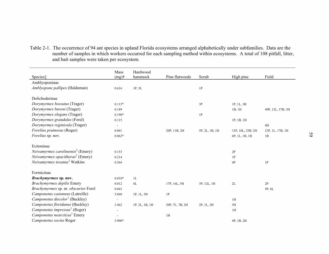
Table 2-1. The occurrence of 94 ant species in upland Florida ecosystems arranged alphabetically under subfamilies. Data are the number of samples in which workers occurred for each sampling method within ecosystems. A total of 108 pitfall, litter, and bait samples were taken per ecosystem.

Species‡ Mass (mg)†

Hardwood hammock Pine flatwoods Scrub High pine Field

Amblyoponinae Amblyopone pallipes (Haldeman) 0.616

1P, 5L 1P Dolichoderinae Dorymyrmex bossutus (Trager) 0.115* 3P 1P, 1L, 3BDorymyrmex bureni (Trager) 0.189 1B, 1H 49P, 12L, 37B, 3H Dorymyrmex elegans (Trager) 0.190* 1PDorymyrmex grandulus (Forel) 0.115 1P, 1B, 1HDorymyrmex reginicula (Trager) - 4H Forelius pruinosus (Roger) 0.061 20P, 11B, 2H 5P, 2L, 1B, 1H 31P, 10L, 25B, 2H 23P, 1L, 17B, 1H Forelius sp. nov. 0.062* 6P, 1L, 1B, 1H 1B Ecitoninae Neivamyrmex carolinensis2 (Emery) 0.153 2PNeivamyrmex opacithorax2 (Emery) 0.214 1PNeivamyrmex texanus2 Watkins 0.564 4P 1P Formicinae Brachymyrmex sp. nov. 0.010* 1LBrachymyrmex depilis Emery 0.012 4L 17P, 16L, 5H 3P, 12L, 1H 2L 2P Brachymyrmex sp. nr. obscurior Forel 0.043 5P, 6LCamponotus castaneus (Latreille) 5.860 1P, 1L, 3H 1P Camponotus discolor1 (Buckley) - 1H Camponotus floridanus (Buckley) 3.462 1P, 2L, 1B, 1H 20P, 7L, 7B, 2H 2P, 1L, 2H 5H Camponotus impressus1 (Roger) - 1H Camponotus nearcticus1 Emery - 1H Camponotus socius Roger 5.900* 4P, 1B, 2H

59

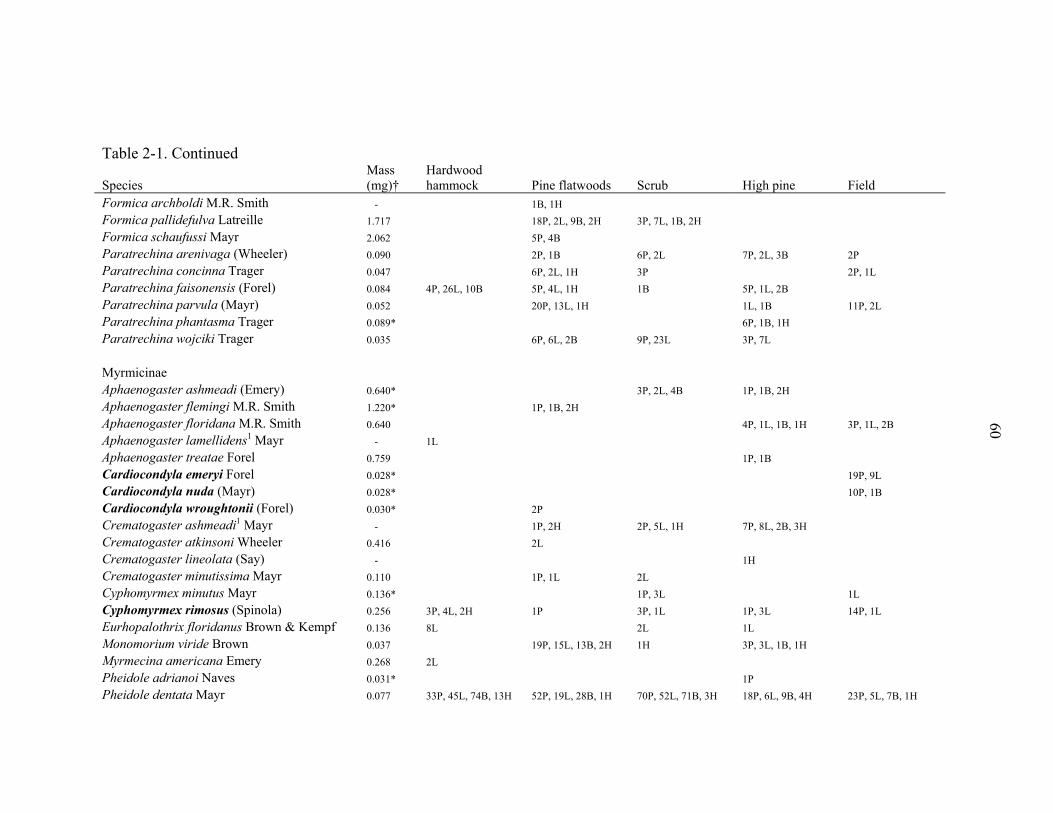
60

Table 2-1. Continued

Species Mass (mg)†

Hardwood hammock Pine flatwoods Scrub High pine Field

Formica archboldi M.R. Smith - 1B, 1H Formica pallidefulva Latreille 1.717 18P, 2L, 9B, 2H 3P, 7L, 1B, 2H Formica schaufussi Mayr 2.062

5P, 4BParatrechina arenivaga (Wheeler) 0.090 2P, 1B 6P, 2L 7P, 2L, 3B 2P Paratrechina concinna Trager 0.047 6P, 2L, 1H 3P 2P, 1L Paratrechina faisonensis (Forel) 0.084 4P, 26L, 10B 5P, 4L, 1H 1B 5P, 1L, 2B Paratrechina parvula (Mayr) 0.052 20P, 13L, 1H 1L, 1B 11P, 2L Paratrechina phantasma Trager 0.089* 6P, 1B, 1HParatrechina wojciki Trager 0.035 6P, 6L, 2B 9P, 23L 3P, 7L Myrmicinae Aphaenogaster ashmeadi (Emery) 0.640* 3P, 2L, 4B 1P, 1B, 2H Aphaenogaster flemingi M.R. Smith 1.220* 1P, 1B, 2H Aphaenogaster floridana M.R. Smith 0.640 4P, 1L, 1B, 1H 3P, 1L, 2B Aphaenogaster lamellidens1 Mayr - 1L Aphaenogaster treatae Forel 0.759 1P, 1BCardiocondyla emeryi Forel 0.028* 19P, 9LCardiocondyla nuda (Mayr) 0.028* 10P, 1BCardiocondyla wroughtonii (Forel) 0.030* 2PCrematogaster ashmeadi1 Mayr - 1P, 2H 2P, 5L, 1H 7P, 8L, 2B, 3H Crematogaster atkinsoni Wheeler 0.416 2LCrematogaster lineolata (Say) - 1H Crematogaster minutissima Mayr 0.110 1P, 1L 2LCyphomyrmex minutus Mayr 0.136* 1P, 3L 1LCyphomyrmex rimosus (Spinola) 0.256 3P, 4L, 2H 1P 3P, 1L 1P, 3L 14P, 1L Eurhopalothrix floridanus Brown & Kempf 0.136 8L 2L 1LMonomorium viride Brown 0.037 19P, 15L, 13B, 2H 1H 3P, 3L, 1B, 1H Myrmecina americana Emery 0.268 2LPheidole adrianoi Naves 0.031* 1PPheidole dentata Mayr 0.077 33P, 45L, 74B, 13H 52P, 19L, 28B, 1H 70P, 52L, 71B, 3H 18P, 6L, 9B, 4H 23P, 5L, 7B, 1H

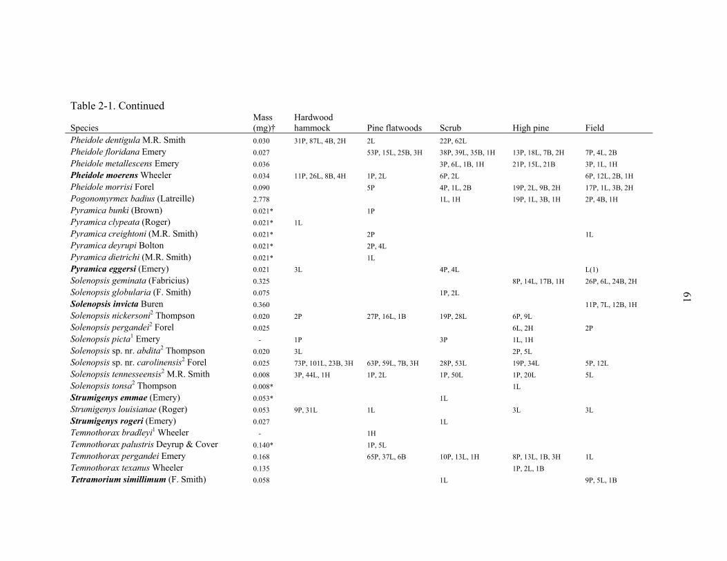
61

Table 2-1. Continued

Species Mass (mg)†

Hardwood hammock Pine flatwoods Scrub High pine Field

Pheidole dentigula M.R. Smith 0.030 31P, 87L, 4B, 2H 2L 22P, 62L Pheidole floridana Emery 0.027 53P, 15L, 25B, 3H 38P, 39L, 35B, 1H 13P, 18L, 7B, 2H 7P, 4L, 2B Pheidole metallescens Emery 0.036 3P, 6L, 1B, 1H 21P, 15L, 21B 3P, 1L, 1H Pheidole moerens Wheeler 0.034 11P, 26L, 8B, 4H 1P, 2L 6P, 2L 6P, 12L, 2B, 1H Pheidole morrisi Forel 0.090 5P 4P, 1L, 2B 19P, 2L, 9B, 2H 17P, 1L, 3B, 2H Pogonomyrmex badius (Latreille) 2.778 1L, 1H 19P, 1L, 3B, 1H 2P, 4B, 1H Pyramica bunki (Brown) 0.021*

1PPyramica clypeata (Roger) 0.021* 1LPyramica creightoni (M.R. Smith) 0.021* 2P 1LPyramica deyrupi Bolton 0.021* 2P, 4LPyramica dietrichi (M.R. Smith) 0.021* 1LPyramica eggersi (Emery) 0.021 3L 4P, 4L L(1)Solenopsis geminata (Fabricius) 0.325 8P, 14L, 17B, 1H 26P, 6L, 24B, 2H Solenopsis globularia (F. Smith) 0.075 1P, 2LSolenopsis invicta Buren 0.360 11P, 7L, 12B, 1HSolenopsis nickersoni2 Thompson 0.020 2P 27P, 16L, 1B 19P, 28L 6P, 9L Solenopsis pergandei2 Forel 0.025 6L, 2H 2PSolenopsis picta1 Emery - 1P 3P 1L, 1H Solenopsis sp. nr. abdita2 Thompson 0.020 3L 2P, 5LSolenopsis sp. nr. carolinensis2 Forel 0.025 73P, 101L, 23B, 3H 63P, 59L, 7B, 3H 28P, 53L 19P, 34L 5P, 12L Solenopsis tennesseensis2 M.R. Smith 0.008 3P, 44L, 1H 1P, 2L 1P, 50L 1P, 20L 5L Solenopsis tonsa2 Thompson 0.008* 1LStrumigenys emmae (Emery) 0.053* 1LStrumigenys louisianae (Roger) 0.053 9P, 31L 1L 3L 3LStrumigenys rogeri (Emery) 0.027 1LTemnothorax bradleyi1 Wheeler - 1H Temnothorax palustris Deyrup & Cover 0.140* 1P, 5LTemnothorax pergandei Emery 0.168 65P, 37L, 6B 10P, 13L, 1H 8P, 13L, 1B, 3H 1L Temnothorax texanus Wheeler 0.135 1P, 2L, 1BTetramorium simillimum (F. Smith) 0.058 1L 9P, 5L, 1B

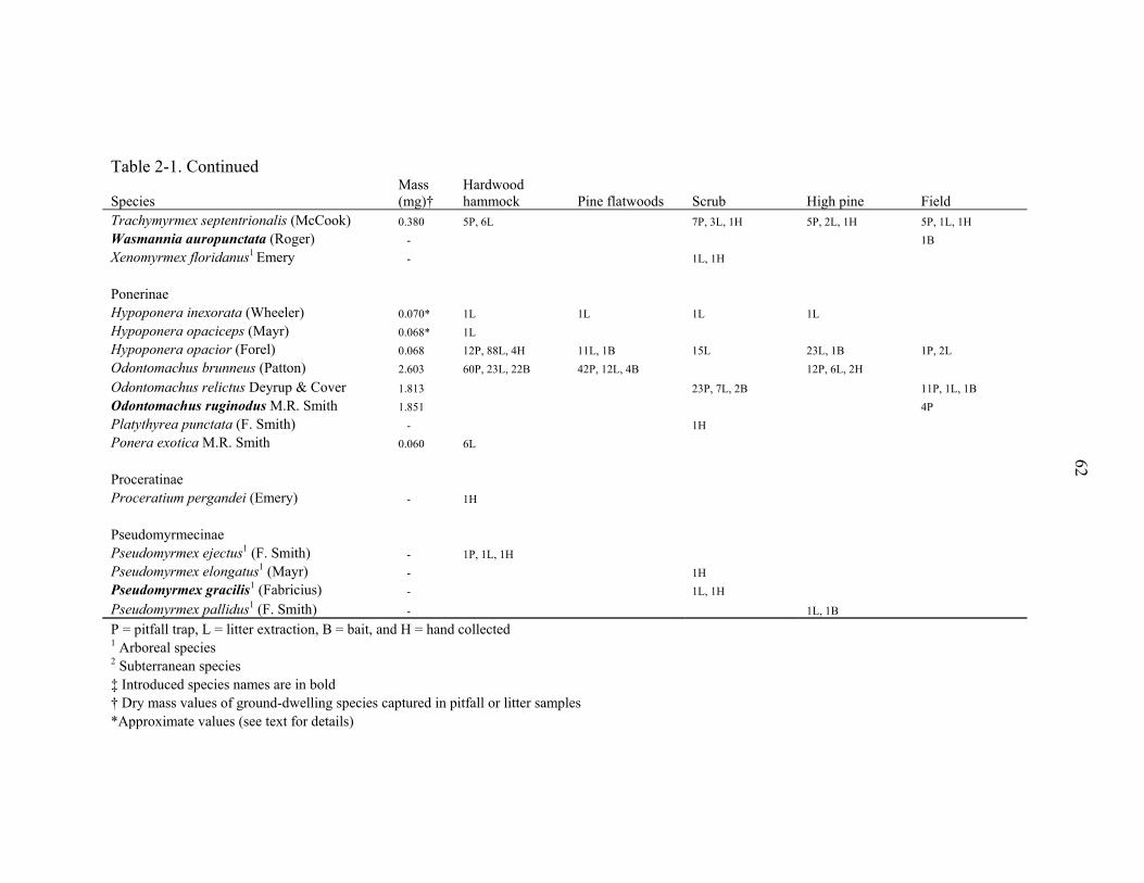
62

Table 2-1. Continued

Species Mass (mg)†

Hardwood hammock Pine flatwoods Scrub High pine Field

Trachymyrmex septentrionalis (McCook) 0.380 5P, 6L 7P, 3L, 1H 5P, 2L, 1H 5P, 1L, 1H Wasmannia auropunctata (Roger) - 1B Xenomyrmex floridanus1 Emery - 1L, 1H

Ponerinae Hypoponera inexorata (Wheeler) 0.070* 1L 1L 1L 1LHypoponera opaciceps (Mayr) 0.068* 1LHypoponera opacior (Forel) 0.068 12P, 88L, 4H 11L, 1B 15L 23L, 1B 1P, 2L Odontomachus brunneus (Patton) 2.603 60P, 23L, 22B 42P, 12L, 4B 12P, 6L, 2H Odontomachus relictus Deyrup & Cover 1.813 23P, 7L, 2B 11P, 1L, 1B Odontomachus ruginodus M.R. Smith 1.851 4PPlatythyrea punctata (F. Smith) - 1H Ponera exotica M.R. Smith 0.060 6L Proceratinae Proceratium pergandei (Emery) - 1H Pseudomyrmecinae Pseudomyrmex ejectus1 (F. Smith) - 1P, 1L, 1H Pseudomyrmex elongatus1 (Mayr) - 1H Pseudomyrmex gracilis1 (Fabricius) - 1L, 1H

Pseudomyrmex pallidus1 (F. Smith) - 1L, 1B

P = pitfall trap, L = litter extraction, B = bait, and H = hand collected 1 Arboreal species

2 Subterranean species ‡ Introduced species names are in bold † Dry mass values of ground-dwelling species captured in pitfall or litter samples *Approximate values (see text for details)

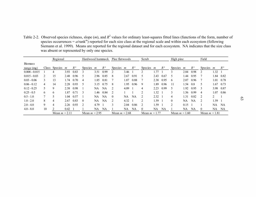
Table 2-2. Observed species richness, slope (m), and R2 values for ordinary least-squares fitted lines (functions of the form, number of species occurrences = a/rankm) reported for each size class at the regional scale and within each ecosystem (following Siemann et al. 1999). Means are reported for the regional dataset and for each ecosystem. NA indicates that the size class was absent or represented by only one species.

Regional Hardwood hammock Pine flatwoods Scrub High pine FieldBiomass range (mg) Class Species m R ² Species m R ² Species m R ² Species m R ² Species m R ² Species m R ²0.008 - 0.015 1 4 3.93 0.83 3 3.51 0.99 2 3.46 1 2 1.77 1 3 2.84 0.98 2 1.32 10.015 - 0.03 2 15 2.48 0.96 5 2.96 0.85 8 2.67 0.91 5 2.43 0.67 5 1.44 0.95 7 1.84 0.820.03 - 0.06 3 13 1.74 0.70 4 1.85 0.81 7 1.87 0.88 7 2.38 0.95 6 2.07 0.96 7 1.01 0.780.06 - 0.12 4 14 2.28 0.93 5 3.15 0.75 8 1.95 0.96 9 1.89 0.96 11 1.54 0.8 5 1.67 0.730.12 - 0.25 5 9 2.38 0.98 1 NA NA 2 4.09 1 4 2.23 0.99 5 1.92 0.95 3 3.98 0.870.25 - 0.5 6 6 1.87 0.71 3 1.46 0.84 2 1 1 2 1.32 1 3 1.56 0.99 4 1.07 0.860.5 - 1.0 7 5 1.04 0.57 1 NA NA 0 NA NA 2 2.32 1 4 1.31 0.82 2 2 11.0 - 2.0 8 4 2.67 0.83 0 NA NA 2 4.32 1 2 1.59 1 0 NA NA 2 1.59 12.0 - 4.0 9 4 2.26 0.93 2 4.79 1 3 2.04 0.86 2 1.59 1 2 0.15 1 1 NA NA4.0 - 8.0 10 2 0.42 1 1 NA NA 1 NA NA 0 NA NA 1 NA NA 0 NA NA

Mean m = 2.11 Mean m = 2.95 Mean m = 2.68 Mean m = 1.77 Mean m = 1.60 Mean m = 1.81

63

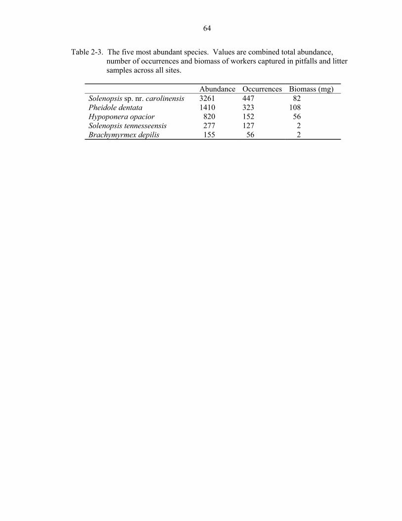
64

Table 2-3. The five most abundant species. Values are combined total abundance, number of occurrences and biomass of workers captured in pitfalls and litter samples across all sites.

Abundance Occurrences Biomass (mg) Solenopsis sp. nr. carolinensis 3261 447 82 Pheidole dentata 1410 323 108 Hypoponera opacior 820 152 56 Solenopsis tennesseensis 277 127 2 Brachymyrmex depilis 155 56 2

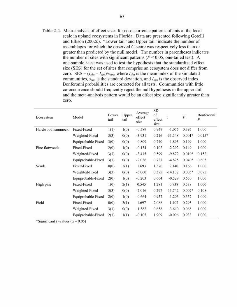
65

Table 2-4. Meta-analysis of effect sizes for co-occurrence patterns of ants at the local scale in upland ecosystems in Florida. Data are presented following Gotelli and Ellison (2002b). “Lower tail” and Upper tail” indicate the number of assemblages for which the observed C-score was respectively less than or greater than predicted by the null model. The number in parentheses indicates the number of sites with significant patterns (P < 0.05, one-tailed test). A one-sample t-test was used to test the hypothesis that the standardized effect size (SES) for the set of sites that comprise an ecosystem does not differ from zero. SES = (Iobs – Isim)/ssim, where Isim is the mean index of the simulated communities, ssim is the standard deviation, and Iobs is the observed index. Bonferonni probabilities are corrected for all tests. Communities with little co-occurrence should frequently reject the null hypothesis in the upper tail, and the meta-analysis pattern would be an effect size significantly greater than zero.

Ecosystem Model Lower tail

Upper tail

Average effect size

SD of effect size

t P Bonferonni P

Hardwood hammock Fixed-Fixed 1(1) 1(0) -0.589 0.949 -1.075 0.395 1.000 Weighted-Fixed 3(3) 0(0) -3.931 0.216 -31.548 0.001* 0.015* Equiprobable-Fixed 3(0) 0(0) -0.809 0.740 -1.893 0.199 1.000 Pine flatwoods Fixed-Fixed 2(0) 1(0) -0.134 0.102 -2.292 0.149 1.000 Weighted-Fixed 3(3) 0(0) -3.415 0.599 -9.872 0.010* 0.152 Equiprobable-Fixed 3(1) 0(0) -2.026 0.727 -4.825 0.040* 0.605 Scrub Fixed-Fixed 0(0) 3(1) 1.693 1.370 2.140 0.166 1.000 Weighted-Fixed 3(3) 0(0) -3.060 0.375 -14.132 0.005* 0.075 Equiprobable-Fixed 2(0) 1(0) -0.203 0.664 -0.529 0.650 1.000 High pine Fixed-Fixed 1(0) 2(1) 0.545 1.281 0.738 0.538 1.000 Weighted-Fixed 3(3) 0(0) -2.016 0.297 -11.742 0.007* 0.108 Equiprobable-Fixed 2(0) 1(0) -0.664 0.957 -1.203 0.352 1.000 Field Fixed-Fixed 0(0) 3(1) 1.697 2.088 1.407 0.295 1.000 Weighted-Fixed 3(1) 0(0) -1.382 0.658 -3.640 0.068 1.000 Equiprobable-Fixed 2(1) 1(1) -0.105 1.909 -0.096 0.933 1.000 *Significant P-values (α = 0.05)

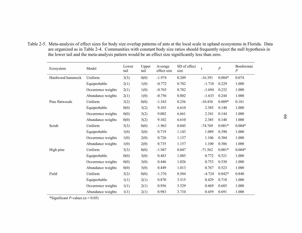
Table 2-5. Meta-analysis of effect sizes for body size overlap patterns of ants at the local scale in upland ecosystems in Florida. Data are organized as in Table 2-4. Communities with constant body size ratios should frequently reject the null hypothesis in the lower tail and the meta-analysis pattern would be an effect size significantly less than zero.

66

Ecosystem Model Lower tail

Upper tail

Average effect size

SD of effect size t P Bonferonni

P

Hardwood hammock Uniform 3(3) 0(0) -1.974 0.209 -16.391 0.004* 0.074 Equiprobable 2(1) 1(0) -0.772 0.782 -1.710 0.229 1.000 Occurrence weights 2(1) 1(0) -0.765 0.782 -1.694 0.232 1.000 Abundance weights 2(1) 1(0) -0.756 0.802 -1.633 0.244 1.000 Pine flatwoods Uniform 3(2) 0(0) -1.543 0.256 -10.436 0.009* 0.181 Equiprobable 0(0) 3(2) 9.103 6.610 2.385 0.140 1.000 Occurrence weights 0(0) 3(2) 9.002 6.661 2.341 0.144 1.000 Abundance weights 0(0) 3(2) 9.102 6.610 2.385 0.140 1.000 Scrub

Uniform 3(3) 0(0) -1.963 0.045 -74.769 0.001* 0.004* Equiprobable 1(0) 2(0) 0.719 1.143 1.089 0.390 1.000 Occurrence weights 1(0) 2(0) 0.726 1.137 1.106 0.384 1.000 Abundance weights 1(0) 2(0) 0.735 1.157 1.100 0.386 1.000 High pine Uniform 3(3) 0(0) -1.947 0.047 -71.562 0.001* 0.004* Equiprobable 0(0) 3(0) 0.483 1.085 0.772 0.521 1.000 Occurrence weights 0(0) 3(0) 0.446 1.026 0.753 0.530 1.000 Abundance weights 0(0) 3(0) 0.449 1.013 0.767 0.523 1.000 Field Uniform 3(2) 0(0) -1.376 0.504 -4.724 0.042* 0.840 Equiprobable 1(1) 2(1) 0.870 3.515 0.429 0.710 1.000 Occurrence weights 1(1) 2(1) 0.956 3.529 0.469 0.685 1.000 Abundance weights 1(1) 2(1) 0.983 3.710 0.459 0.691 1.000 *Significant P-values (α = 0.05)

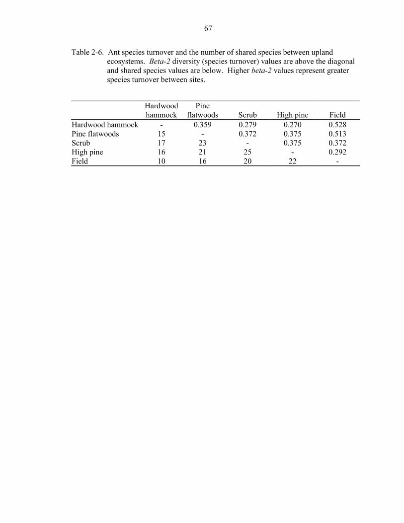
67

Table 2-6. Ant species turnover and the number of shared species between upland ecosystems. Beta-2 diversity (species turnover) values are above the diagonal and shared species values are below. Higher beta-2 values represent greater species turnover between sites.

Hardwood hammock

Pine flatwoods Scrub High pine Field

Hardwood hammock - 0.359 0.279 0.270 0.528 Pine flatwoods 15 - 0.372 0.375 0.513 Scrub 17 23 - 0.375 0.372 High pine 16 21 25 - 0.292 Field 10 16 20 22 -

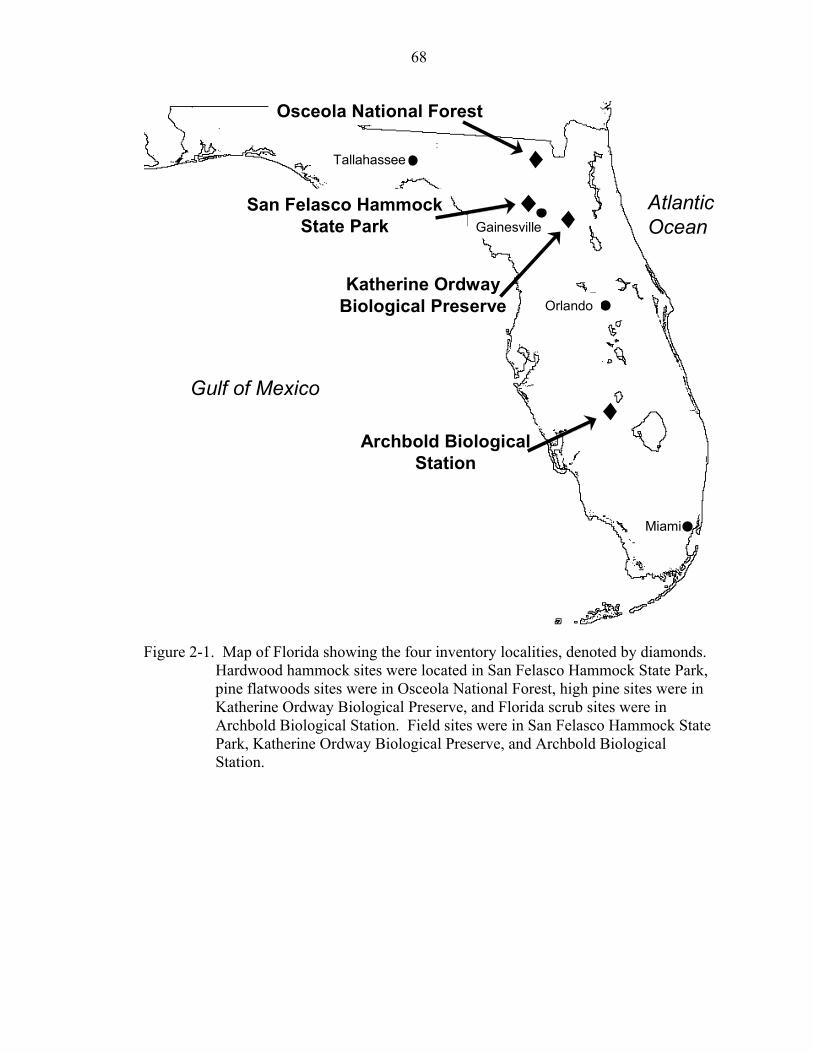
68

Tallahassee

Gainesville

Miami

AtlanticOcean

Gulf of Mexico

Osceola National Forest

Katherine OrdwayBiological Preserve

San Felasco HammockState Park

Archbold BiologicalStation

Orlando

Tallahassee

Gainesville

Miami

AtlanticOcean

Gulf of Mexico

Osceola National Forest

Katherine OrdwayBiological Preserve

San Felasco HammockState Park

Archbold BiologicalStation

Orlando

Figure 2-1. Map of Florida showing the four inventory localities, denoted by diamonds.

Hardwood hammock sites were located in San Felasco Hammock State Park, pine flatwoods sites were in Osceola National Forest, high pine sites were in Katherine Ordway Biological Preserve, and Florida scrub sites were in Archbold Biological Station. Field sites were in San Felasco Hammock State Park, Katherine Ordway Biological Preserve, and Archbold Biological Station.

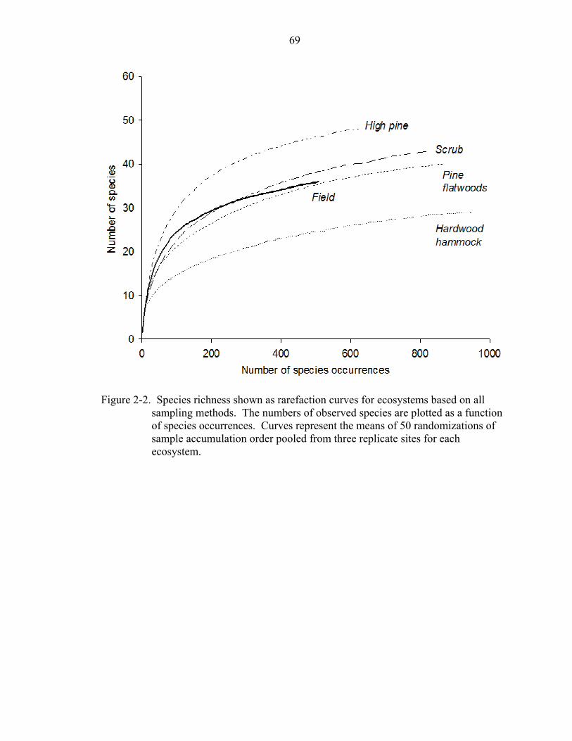
69

Figure 2-2. Species richness shown as rarefaction curves for ecosystems based on all

sampling methods. The numbers of observed species are plotted as a function of species occurrences. Curves represent the means of 50 randomizations of sample accumulation order pooled from three replicate sites for each ecosystem.

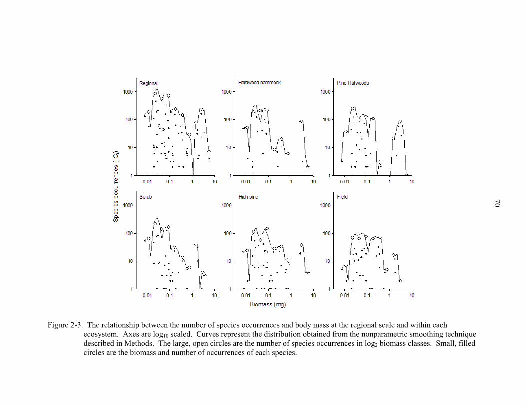
70

Figure 2-3. The relationship between the number of species occurrences and body mass at the regional scale and within each

ecosystem. Axes are log10 scaled. Curves represent the distribution obtained from the nonparametric smoothing technique described in Methods. The large, open circles are the number of species occurrences in log2 biomass classes. Small, filled circles are the biomass and number of occurrences of each species.

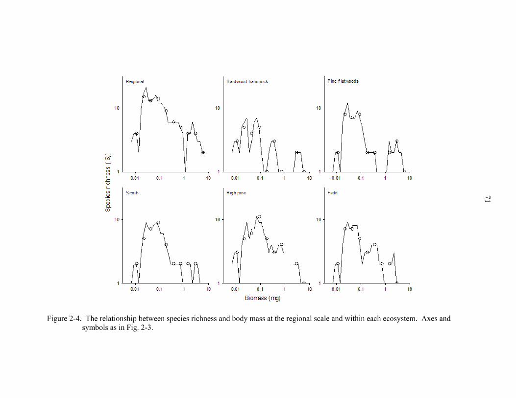
71

Figure 2-4. The relationship between species richness and body mass at the regional scale and within each ecosystem. Axes and

symbols as in Fig. 2-3.

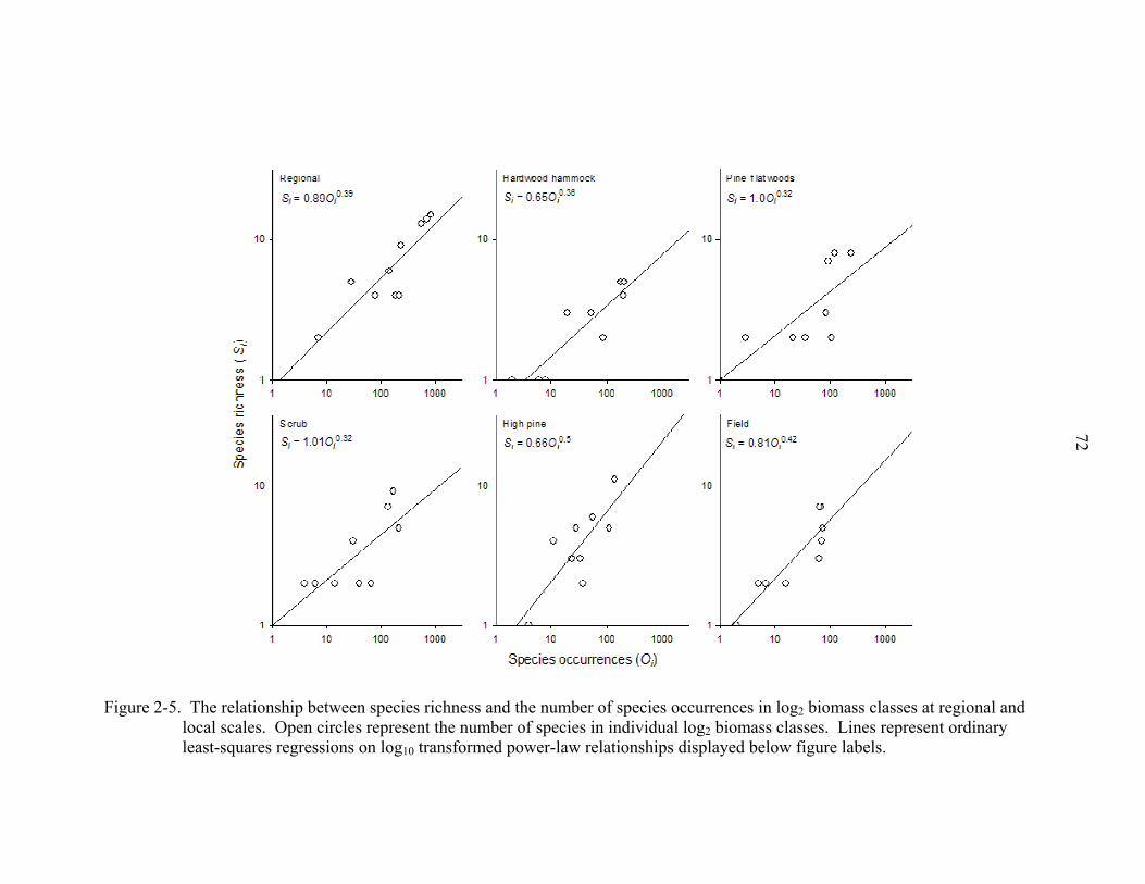
72

Figure 2-5. The relationship between species richness and the number of species occurrences in log2 biomass classes at regional and

local scales. Open circles represent the number of species in individual log2 biomass classes. Lines represent ordinary least-squares regressions on log10 transformed power-law relationships displayed below figure labels.

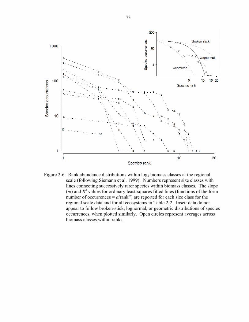
73

Figure 2-6. Rank abundance distributions within log2 biomass classes at the regional

scale (following Siemann et al. 1999). Numbers represent size classes with lines connecting successively rarer species within biomass classes. The slope (m) and R2 values for ordinary least-squares fitted lines (functions of the form number of occurrences = a/rankm) are reported for each size class for the regional scale data and for all ecosystems in Table 2-2. Inset: data do not appear to follow broken-stick, lognormal, or geometric distributions of species occurrences, when plotted similarly. Open circles represent averages across biomass classes within ranks.

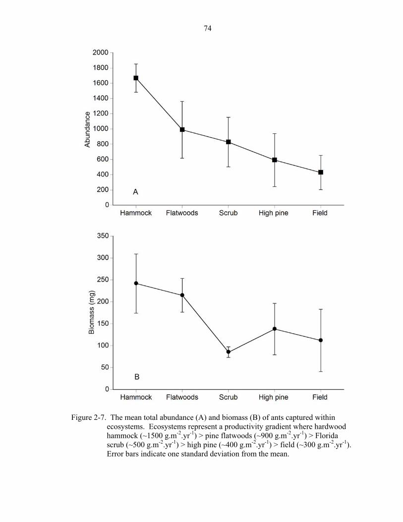
74

Figure 2-7. The mean total abundance (A) and biomass (B) of ants captured within

ecosystems. Ecosystems represent a productivity gradient where hardwood hammock (~1500 g.m-2.yr-1) > pine flatwoods (~900 g.m-2.yr-1) > Florida scrub (~500 g.m-2.yr-1) > high pine (~400 g.m-2.yr-1) > field (~300 g.m-2.yr-1). Error bars indicate one standard deviation from the mean.

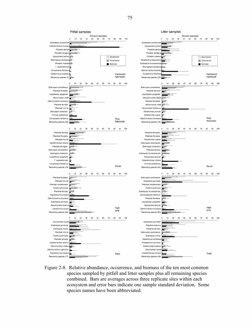
75

Figure 2-8. Relative abundance, occurrence, and biomass of the ten most common

species sampled by pitfall and litter samples plus all remaining species combined. Bars are averages across three replicate sites within each ecosystem and error bars indicate one sample standard deviation. Some species names have been abbreviated.

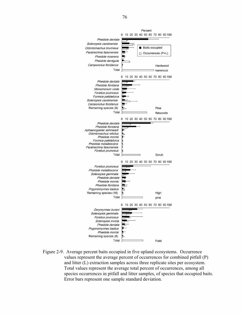
76

Figure 2-9. Average percent baits occupied in five upland ecosystems. Occurrence

values represent the average percent of occurrences for combined pitfall (P) and litter (L) extraction samples across three replicate sites per ecosystem. Total values represent the average total percent of occurrences, among all species occurrences in pitfall and litter samples, of species that occupied baits. Error bars represent one sample standard deviation.

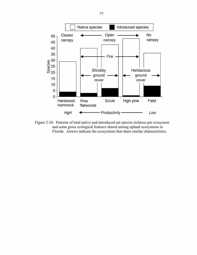
77

Figure 2-10. Patterns of total native and introduced ant species richness per ecosystem

and some gross ecological features shared among upland ecosystems in Florida. Arrows indicate the ecosystems that share similar characteristics.

CHAPTER 3 EVALUATION OF SAMPLING METHODS AND SPECIES RICHNESS ESTIMATORS FOR ANTS IN UPLAND ECOSYSTEMS IN FLORIDA

Introduction

Biological inventory is a fundamental component of natural science. Inventories

provide the foundation for improving the applied pursuits of sustainable resource

management, conservation biology, and pest management (Price and Waldbauer 1994,

New 1998). Appreciation of the importance of biological inventory and the value of

biodiversity has steadily grown in the last two decades as the potential impact of the

biodiversity crisis has been recognized (Wilson 1988, Raven and Wilson 1992). For

many terrestrial vertebrates and some plants, intensive local or regional sampling can be

expected to produce a comprehensive inventory when integrated with existing

information such as the taxon-based work of systematists (Eldredge 1992). However, for

the vast majority of terrestrial organisms, particularly hyperdiverse groups such as

arthropods, a relatively comprehensive inventory is difficult to achieve except at very

small scales or in isolated regions with depauperate faunas (e.g., small oceanic islands,

Disney 1986).

The goal of most arthropod inventories commonly falls into one of two categories:

strict inventory or community characterization (sensu Longino and Colwell 1997). Strict

inventory generates a relatively comprehensive species list for a discrete spatiotemporal

unit, which requires species-level identification of samples (Longino and Colwell 1997).

Comparisons with other spatiotemporal units are not necessarily desirable. Traditionally,

78

79

strict inventories have been carried out by systematists and museum collectors. In

contrast, community characterization uses structured sampling (i.e., randomization and

repetition) to permit statistical separation of different spatiotemporal units. This is done

for the purposes of ranking units according to the goals of conservation or pest

management (Cochran 1963, Longino and Colwell 1997). Unit ranking may not require

sample identifications to the species level because the primary concern is the relative

abundances of focal taxa and how they change across space or time (Colwell and

Coddington 1994, Oliver and Beattie 1996). Normally, community characterization is

carried out using one or a few sampling techniques and comprehensive species lists are

neither necessary nor feasible (Disney 1986, Longino and Colwell 1997). Community

characterization has most often been used by entomologists, ecologists, and conservation

biologists.

Recently, analytical advances focused on examining arthropod ecology have

converged with a growing emphasis on including arthropods in rapid biodiversity surveys

for conservation purposes (Wilson 1988, Coddington et al. 1991, Kim 1993, Colwell and

Coddington 1994, Kremen 1992, 1994, Kremen et al. 1993, Silva and Coddington 1996,

Longino and Colwell 1997, New 1998, Fisher 1999a, Anderson and Ashe 2000, Gotelli

and Colwell 2001, Sørensen et al. 2002). Accordingly, a number of taxon-specific,

structured inventory techniques have been introduced which utilize a variety of sampling

methods that combine the “species hunting” techniques of systematists with the more

quantitative methods of ecologists (Coddington et al. 1991, Longino and Colwell 1997,

Fisher 1999a). This approach serves as a practical, short-term alternative to long-term,

comprehensive surveys (e.g., Deyrup and Trager 1986, Lawton et al. 1998) for assessing

80

local arthropod diversity. By design, this methodology combines the quantitative

approach of community characterization with the objectives of strict inventory. It

permits analyses of inventory completeness and an assessment of the costs and benefits

of methods when used individually and in combination (Longino and Colwell 1997,

Fisher 1999a, Delabie et al. 2000).

To assess inventory methods, an account of species captured per sampling method

as well as per unit area or time is necessary to evaluate effectiveness. Species

accumulation curves are an effective method for evaluating the efficiency of various

inventory techniques for sampling species richness (Clench 1979, Soberón and Llorente

1993, Colwell and Coddington 1994). A species accumulation curve is a plot of the

cumulative number of species discovered within a defined area (and/or time) as a

function of some measure of effort. Curves can be constructed to measure either species

density (the number of species per unit area) or species richness (the number of species

per individual, Gotelli and Colwell 2001). Species accumulation curves are similar to

rarefaction curves (sensu Gotelli and Colwell 2001) which are produced by randomly and

repeatedly re-sampling a pool of individuals or samples and plotting the number of

species represented by increasing numbers of individuals. In fact, rarefaction curves can

be viewed as the statistical expectation of a corresponding species accumulation curve

when samples are repeatedly reordered (Gotelli and Colwell 2001).

When the actual number of species in an area is unknown (as is typically the case

for arthropods) the shape of a rarefaction curve can be used to estimate how completely

an area has been sampled and how efficiently different methods have captured species in

that area (Colwell and Coddington 1994, Longino and Colwell 1997, Fisher 1999a). A

81

curve that approaches an asymptote after a large sampling effort is representative of a

decrease in species accrual – a measure of sampling completeness (Colwell and

Coddington 1994, Longino and Colwell 1997, Gotelli and Colwell 2001). Sampling

completeness can be further evaluated by comparing curve asymptotes with values

determined by species richness estimators or by observed species richness from well-

sampled localities. When used in combination with a structured inventory, rarefaction

curves are intended to permit quantitative analyses of species richness for comparison

between methods or between sites. Additionally, subsamples can be evaluated within the

context of the entire data set to determine the relative efficiency of method combinations

and changes in design (e.g., the effect of increasing distance between samples) (Fisher

1999a).

Among arthropods, ants (Hymenoptera: Formicidae) have been a focal group for

development of structured inventory protocols and novel techniques for analyzing data

generated from structured inventory. Ants are an appropriate group for testing the

effectiveness of new methods. They are diverse, abundant, and nearly ubiquitous. They

influence the biotic and abiotic processes of the ecosystems where they occur. A

majority of species nest in fixed positions, largely ensuring that species dwell where they

are sampled. They are among the most studied terrestrial invertebrate taxa and have been

used to monitor environmental impact and ecosystem recovery (Andersen 1990, 1993,

Hölldobler and Wilson 1990, Folgarait 1998). Numerous, established sampling

techniques are available, representing a range of costs and yields (Bestelmeyer et al.

2000). Furthermore, structured inventory techniques and biodiversity data analyses have

been established for inventorying and estimating ant species richness in tropical

82

rainforest ecosystems (Longino and Colwell 1997, Fisher 1996, 1998, 1999a, b, 2002,

Agosti et al. 2000a, b, Longino et al. 2002). Much less is known about the performance

of structured inventory methods to capture ants in subtropical and temperate ecosystems.

Similarly, the performance of species richness estimators remains largely untested on

data drawn from temperate or subtropical ant communities. The biodiversity crisis is not

confined to the tropics (Platnick1992) and neither are the goals of conservation biology

and ecology. Accordingly, improving structured inventory methods and species richness

estimation for ants and arthropods in a variety of ecosystems is warranted.

In this study, I evaluated the efficiency of a structured inventory of ants in northern

and central Florida. In so doing, I compared the efficiency of four individual sampling

methods and the performance of three species richness estimation techniques. The ant

fauna of Florida has been thoroughly surveyed in the past 50 years throughout the state

(Van Pelt 1956, 1958, Deyrup and Trager 1986, Deyrup et al. 2000, Lubertazzi and

Tschinkel 2003, M. Deyrup, L. Davis, Z. Prusak, S. Cover, J.R. King unpublished data).

As a result, there is a clear record of distribution and habitat association for a majority of

species (Deyrup 2003). Consequently, this study presented a unique opportunity to

compare inventory results and species richness estimations with approximate species

richness values expected at local and regional scales. In evaluating sampling methods my

objectives were to compare: (1) the number of ant species captured by baits, pitfalls,

litter-extraction, and hand-collecting methods (and combinations thereof) in five different

ecosystems, (2) the complementarity of sampling methods, and (3) the relative costs (in

time) of sampling methods. These objectives permit an analysis of the efficiency of

sampling methods in the context of facilitating conservation or land-planning decisions

83

that require comparable estimates of species richness and endemism (Coddington et al.

1991, Platnick 1992).

Methods

Study Area

A detailed description of the ecosystems sampled and the methods used in this

study can be found in Chapter 2. Briefly, this study was carried out in three sites in each

of five different ecosystems (a total of 15 study sites) in north and central Florida.

Sampling was performed in temperate hardwood forests in the San Felasco Hammock

State Park, pine flatwoods in the Osceola National Forest, high pine in the Katherine

Ordway Biological Preserve, and Florida scrub forest in the Archbold Biological Station.

The plant community descriptions of Myers and Ewel (1990a) were used as a basis for

ecosystem selection. These sites were selected a priori as they contain some of the

remaining relatively undisturbed native upland ecosystems in Florida. I also sampled a

non-native ecosystem, consisting of converted (previously cleared) fields, to represent

moderately disturbed habitat. A field was sampled in an area adjacent to natural areas at

San Felasco Hammock State Park, the Katherine Ordway Biological Preserve, and the

Archbold Biological Station. The ecosystems sampled represent a gradient of upland

plant communities that include closed-canopy, hardwood forests, open-canopy pine and

oak woodland, and completely open, herbaceous savannah.

Sampling

Ants were sampled from June through September, 2001 using baits, pitfall traps,

leaf-litter extraction with Berlese funnels, and hand collecting. A total of 36 pitfall traps

and 36 litter samples were placed separately at 5m intervals (180 m, total) in two parallel

lines separated by 10 m (Fisher 1996, 1998, 1999b, 2002). A transect of 36 baits was

84

placed between the pitfall and litter extraction lines with each bait corresponding to

pitfall and litter extraction samples. Pitfall traps were 85 mm long plastic vials with 30

mm internal diameter partially filled with ~ 15 mm of propylene-glycol antifreeze. Traps

were buried with the open end flush with the surface of the ground and operated for 3

days. Two 0.25 m2 litter samples were taken after setting pitfall traps at each litter sample

point. Litter samples were obtained by collecting all surface material and the first ~ 1 cm

of soil within quadrats. The two samples were pooled, larger objects (e.g., logs)

macerated with a machete, and sifted through a sieve with 1 cm grid size. Sifted litter was

placed in covered metal 32 cm diameter Berlese funnels under 40 watt light bulbs. The

funnels were operated until the samples were dry (~ 48 to 72 h). Baits were 12 ×75 mm

test tubes with a piece (~ 2 g) of hot dog (Oscar Meyer® beef franks, Northfield, Illinois)

inserted ~ 2 cm into the tube. At each sampling point, a small spot was cleared of any

litter and the bait tube was placed directly on the ground (to speed discovery and access),

and shaded with one half of a Styrofoam plate. The baits were operated for 0.5 h,

collected, and the ends plugged with small cotton balls to prevent the ants from escaping.

Hand collecting consisted of systematically searching vegetation, tree trunks, logs, and

small twigs for 2 h per site. Hand collecting was performed within and immediately

adjacent to (~ 5 to 10 m) sites. Time records were kept for each step of the sampling and

sorting process to estimate costs. Time costs included installation, operation, and

collecting of samples, traps and baits, and time spent processing and identifying

specimens. For the sake of technical consistency, and with the exception of one high

pine site, all sampling was performed by J.R. King. Similarly, all ants, from all samples,

were sorted, counted and identified to species by J.R. King.

85

Analysis

All records used in this study were based on the worker caste as their presence

provides evidence of an established colony (Fisher 1999a, Longino et al. 2002). The

purpose of the sampling design was to produce a representative, relatively complete

species list for each ecosystem type. Therefore, data for the three sites sampled within

each ecosystem type were pooled and converted to a species-by-sample incidence

(presence-absence) matrix (Longino 2000, Longino et al. 2002). A regional data set was

also generated by pooling all of the data into a single species by sample incidence matrix.

The relative abundance of individuals is an important measure when considering species

richness (Gotelli and Colwell 2001). For ants, however, the sampled abundance of

foraging workers is not comparable to individuals of other animals. The sociality of ants

can often lead to extreme clumping of individuals within samples (particularly litter

samples, which may include entire colonies) which may skew species richness

comparisons and species/abundance relationships (Gotelli and Colwell 2001). To remedy

this, species occurrences (incidence data) were used in place of the abundance of

individuals when evaluating species-based abundance measures (Longino 2000, Fisher

and Robertson 2002, Longino et al. 2002).

Sample-based rarefaction curves were used to compare total species richness within

ecosystems and for the regional data set. Total species richness captured by each method

in each ecosystem was similarly evaluated. Rarefaction curves were generated by

random re-orderings (50 times) of samples using the program EstimateS (Colwell 2000).

I compared these sample-based rarefaction curves with the observed number of species

plotted on the y-axis (ordinate) against species occurrences (presence/absence data)

plotted on the x-axis (abscissa) to assess differences in species richness between and

86

among curves representing ecosystems and methods (Colwell and Coddington 1994,

Gotelli and Colwell 2001).

Species richness was estimated in three ways for each ecosystem and for the

regional data set: (1) by fitting a lognormal distribution, (2) by extrapolating rarefaction

curves, and (3) by using nonparametric estimators. For the parametric model fitting, the

sample data from each site were fitted to the lognormal distribution using the method of

Preston (1948). In this method, the sample data were fitted to the lognormal

distribution, , where S(R) is the number of species in the R)(0

22

)( RaeSRS −= th octave, S0 is

the number of species in the modal octave, and a is a parameter related to the width of the

distribution. Parameters of the lognormal were estimated using a modified version of

Ludwig and Reynolds (1988) method. Octaves were assigned to abundance classes

(observed) and parameters S0 and a were estimated using nonlinear curve fitting (proc

nlin, Newton’s estimation method and least squares fitting, SAS release 8.02, 2000;

Longino et al. 2002). Species richness was estimated by calculating the total area under

the fitted curve, including the portion of the curve hidden behind the “veil line”

(Magurran 1988).

Projection of the rarefaction curves for the regional data set was accomplished

using sample-based rarefaction plots (Soberón and Llorente 1993, Gotelli and Colwell

2001). Patterns seen in the rarefaction curves generated for individual ecosystems were

similar to those of the regional data set and were not displayed. The smoothed curves

were created by averaging repeated, random reorderings (50 times) of the samples with

the mean number of species occurences from each sample computed in succession

(Colwell and Coddington 1994, Gotelli and Colwell 2001). The smoothed curves were

87

then projected by fitting the asymptotic Michaelis-Menten equation, nBnS

nS+

= max)( ,

where S(n) is the number of species, n is the number of samples, and Smax and B are fitted

constants (Colwell and Coddington 1994). Following Raaijmaker (1987), maximum

likelihood estimators for parameters (Smax and B) were determined for the Eadie-Hofstee

transformation of the equation (Colwell and Coddington 1994, Longino et al. 2002).

I also used two nonparametric methods to estimate species richness for comparison

with the rarefaction curves. A jacknife (henceforth Jack2) estimator

−−

−−

+=)1()2(32( 2

nnnM

nnLSS obs , where L = the number of species in one sample, M =

the number of species that occur in two samples, and n = the number of samples

(Burnham and Overton 1978, 1979). An incidence-based coverage estimator (ICE),

21infice

iceice

rfreqice C

QCSSS γ++= , where Sfreq = number of frequent species (found in more

than 10 samples), Sinfr = number infrequent species (found in less than 10 samples), Cice =

sample incidence coverage estimator, Q1 = frequency of uniques, and = estimated

coefficient of variation of the Q

2iceγ

i for infrequent species (Lee and Chao 1994). These

estimators were chosen as they have been shown to reliably provide intermediate (ICE)

and upper (Jack2) level species richness estimates relative to observed species richness

and other nonparametric estimators in biological inventories (Colwell and Coddington

1994, Chazdon et al. 1998, Sørensen et al. 2002).

All species richness estimates were compared with total species richness values

generated for each ecosystem and the region from previous collection records. These

records included published (Van Pelt 1956, 1958, Deyrup and Trager 1986, Lubertazzi

88

and Tschinkel 2003) and unpublished inventories (Van Pelt 1947, Prusak 1997) and

personal collection data sets (J.R. King, L. Davis, M. Deyrup). Amassed over more than

50 years, these collections represent a relatively comprehensive species occurrence data

set for several localities and the region as a whole. Using these data, a minimum species

richness value was determined for the regional data set by including all of the species

with collection records coinciding with the study area (north-central Florida in the region

stretching from Columbia and Baker Counties southward along the central ridge of the

peninsula to the end of the Lake Wales Ridge in Highlands County). At the scale of the

ecosystem, the minimum species richness estimate was determined from collection

records by determining the highest number of species previously captured by an

approximately similar sampling effort (many samples taken using multiple methods) and

size of study area (e.g. the hardwood hammock within San Felasco Hammock State Park)

used in my study. These values are approximations and represent a minimum.

Nevertheless, the extensive sampling effort (amassed by both systematists and ecologists

utilizing a variety of collecting methods over a long period of time) applied to this region

ensures that these are accurate minimum estimates. Similarly, collection records were

used to assess the observed rarity of species collected in this study. Species that were

unique to either the study as a whole (uniques) or to individual sampling methods were

compared to collection records to determine whether the rarity of these species was a

product of insufficient (or inappropriate) sampling or if they were truly rare.

To assess complementarity among methods, I used a measure that describes the

proportion of all species in two sites that occurs in only one, or the other of both (Colwell

and Coddington 1994). Pairwise complementarity or distinctness values were calculated

89

using the Marczewski-Steinhaus (M-S) distance: jbajbaCMS −+

−+=

2 , where a = the

number of species at site A, b = the number of species at site B, and j = the number of

species common to both. Methods were compared within ecosystems and for the

regional data set. To further analyze the sampling efficiency of quantitative methods,

litter and pitfall data were examined within sites to determine the impact of spatial

separation among sample points on the similarity of species sampled. Within sites,

faunal similarity among samples along each transect was determined using the Jaccard

index: jba

jJ −+

=S (the compliment of the M-S distance). The similarity of samples

for all pairwise combinations of sample points (5 m to 35 m apart) along each transect

was plotted against increasingly larger distances along each site transect to determine the

homogeneity of samples at (Fisher 1999a). These were averaged among sites within each

ecosystem. Comparisons beyond 150 m were excluded from the analysis because there

were increasingly fewer replicates to generate means (e.g., there is only one pairwise

comparison of samples 175 m apart).

I examined the time costs of individual methods. Time costs included time spent in

the field collecting samples and in the laboratory sorting and identifying specimens.

Laboratory hours were spent on tasks that required previous, rigorous scientific training

(e.g., sorting and identifying specimens to the species level). Field hours were an account

of time spent on tasks that did not require specialized training (e.g., laying out pitfalls,

sifting litter). Although the time required to accomplish these tasks would undoubtedly

vary among different workers, a comprehensive account of time costs per method

provides an estimate of the amount of time required to reproduce similar results under

90

similar conditions. The time cost per method would remain consistent relative to the time

costs for the other methods even if, for example, multiple workers were utilizing the same

methods.

Finally, the effectiveness of quantitative methods for predicting total site species

richness was determined. Ordinary least-squared regressions were used to determine the

relationship between total species richness and species richness per method for baits,

pitfalls, and litter samples within sites.

Results

The inventory captured 37,961 individual ants representing 94 species from 31

genera. A total of 3774 species occurrences were distributed among 1732 samples.

Three species [Dorymyrmex elegans (Trager), Paratrechina phantasma Trager, and

Pheidole adrianoi Naves] which are endemic to deep sandy ridges in Georgia and along

the central peninsula of Florida were sampled in high pine and scrub. Twelve arboreal

species and 8 subterranean species were also captured. A species list and detailed

discussion of the relative abundance, body size, and ecology of individual species

captured in this study can be found in Chapter 2.

Observed and Estimated Species Richness

Observed species richness varied among ecosystems. The most species were

captured in high pine and scrub ecosystems while fewer species were captured in pine

flatwoods, field, and hardwood hammock ecosystems, respectively (Table 3-1, observed

species). The species captured included 82 ground-dwelling species (including 8

subterranean species) and 12 arboreal species. At the regional scale, the 94 species

sampled included 20 uniques and 10 duplicates (Fig. 3-1). The sample-based rarefaction

curve of observed species richness approached but did not reach an asymptote. Two-

91

thirds of the species were captured within the first ~ 750 species occurrences. Beyond

750 species occurrences the addition of species was considerably diminished.

The method of lognormal curve fitting to estimate species richness consistently

predicted species richness levels at or only slightly above the observed richness (Fig. 3-1

and Table 3-1). All other richness estimators generally did not stabilize with increasing

sampling effort. As sample size increased, so too did the estimates (Fig. 3-1). Estimators

also consistently predicted widely separated results relative to each other. Projecting the

Michaelis-Menten curve produced estimates at or, most frequently, below observed

species richness. The MMMeans estimate also increased steadily with sample size with

no evidence of leveling off (Fig. 3-1). The ICE consistently predicted species richness

greater than the observed species richness but less than Jack2 estimates. Both ICE and

Jack2 showed some evidence of leveling off between 1500 and 2200 species occurrences,

however, they both became unstable beyond 2200 occurrences, rising steadily with

increasing sample size. Neither uniques nor duplicates showed any sign of decreasing.

Rather, they remained at nearly the same level throughout the majority of the sampling

effort.

The estimates for the completeness of the inventory ranged from 71 to 90% of the

minimum species richness estimates within ecosystems (Table 3-1). Similarly, an

estimated 66% of the total regional fauna was sampled during this study. Within

ecosystems, the ICE and Jack2 estimators were very near the minimum site estimates

predicted from previous survey work. In contrast, MMMeans and lognormal estimates

were little different from observed species richness values. For the regional data set,

92

Jack2 was nearest to the minimum site estimate while all other estimators produced

considerably lower species richness estimates.

Rarity

Uniques accounted for ~ 21% of the total species richness. The 20 uniques

captured in this study included 5 arboreal species (Chapter 2, Table 2-1). All of the

arboreal species captured are common, although not abundant throughout the range of the

study and were poorly sampled by the methods utilized. Similarly, two of the uniques

were subterranean species that are rarely captured, although an alternative sampling

method (subterranean baiting, J.R. King unpublished data) has revealed that one of these

species is common. Five ground-dwelling species among the uniques are frequently

encountered within peninsular Florida although their low abundance here suggests that

they are uncommon in the upland habitats sampled. The remaining eight ground-

dwelling species have not been commonly collected previously, suggesting that these

species are truly uncommon or rare.

Complementarity of Ecosystems

Comparing faunas among different sites revealed that, on average, species

composition was much more similar among sites in the same ecosystem type than among

different ecosystems (Table 3-2). Between different ecosystems the complementarity of

species lists was similar. A similar pattern was also seen among sites of the same

ecosystem with the exception of field sites. Field sites were less similar to one another

than other ecosystems, probably as a result of their geographic separation. The greatest

difference in species composition occurred between pine flatwoods and field sites, while

the least difference was seen between scrub and pine flatwoods sites.

93

Effectiveness of Sampling Methods

Sample-based rarefaction curves for individual methods (Fig. 3-2) revealed that

pitfall and litter samples were nearly identical in the number of species each captured and

both methods captured more species than hand collecting and baiting. This pattern was

consistent within individual ecosystems as well, except for hardwood hammocks (data

not shown). In hardwood hammocks, litter sampling captured a much greater number of

species (26) than pitfalls (17). Baiting was the least productive method for capturing

species richness. The pitfall, litter and combined curves all approached an asymptote

while baiting and hand collecting did not. The combination of quantitative methods

(pitfall, litter, and bait samples) was the most thorough for capturing species richness.

The hand collecting curve shows little evidence for an asymptote at all, indicating a very

rapid increase in species per individual collected and no evidence of an asymptote. The

lack of an asymptote suggests that too little time was spent hand-collecting per site. The

rapid accrual of species by hand collecting and the lack of an asymptote suggest that

collecting in this manner is the most efficient method for maximizing species richness.

However, this is a methodological artifact, because duplicate collections were generally

avoided. Consequently, time, rather than species occurrences, is a better ordinate for

assessing the effectiveness of this method.

Litter and pitfall samples were the most similar in species composition among all

sampling methods (Table 3-2). Baits and litter samples were the least similar in species

composition. Overall, the fauna captured by hand collecting was the least similar in

species composition to any of the other collecting methods. Litter extraction sampling

was particularly useful for capturing cryptic species living in rotting wood and in leaf

litter. Pitfall samples were most effective at capturing highly active, surface foraging

94

species. Hand collecting captured a number of arboreal species that were not captured by

other methods.

Within ecosystems the similarity of samples along 180 m linear transects varied

slightly between nearby and distant samples (Fig. 3-3). Field sites exhibited the most

dissimilarity between nearby and distant sites with a steady decrease in the similarity of

species composition per sample as a function of increasing distance. Sample

autocorrelation differed among ecosystems and methods with hardwood hammock

samples exhibiting greater similarity among samples, on average, than other ecosystems

– particularly among litter samples. Pine flatwoods and scrub ecosystems were most

similar in the degree of sample autocorrelation while hardwood hammock and high pine

were the least similar. With the possible exception of fields, the impact of ecosystem

type seems to be a greater determinant of sample autocorrelation than distance between

samples.

Litter samples required the most time to collect, sort, and process, followed by

pitfalls, baits and hand collected samples, respectively (Fig. 3-4). Baits commonly

produced very large numbers of individuals of the same species, particularly mass

recruiting species such as P. dentata Mayr and Solenopsis invicta Buren. Litter sampling

often captured entire colonies or colony fragments of multiple species, also resulting in

large numbers of individuals. Pitfall samples and hand collecting tended to produce more

species per individual sampled. There were 8 species captured only in pitfall samples, 13

species captured only in litter samples, 8 species captured only by hand collecting, and 1

species captured only by baiting (Fig. 3-4).

95

Pitfall species richness predicted a majority of total site species richness (Fig. 3-5;

total = 3.58 + 1.29pitfall, R2 = 0.69, P < 0.01). Litter species richness accounted for

slightly less of the variability in total species richness (total = 7.47 + 1.04litter, R2 = 0.61,

P < 0.01) and while bait species richness predicted a minority of total site species

richness (total = 15.98 + 1.29bait, R2 = 0.46, P = 0.01) across all sites.

Discussion

The results of this study demonstrate the effectiveness of a structured inventory

approach for effectively sampling temperate or subtropical arthropod communities. They

provide guidance for organizing sampling projects undertaken elsewhere at either local or

regional scales. They also provide guidance for the selection of sampling methods based

upon the characteristics of the ecosystems where sampling is to take place. Additionally,

this study reveals the potential value of structured inventory for use in land-management

and conservation applications where rapidly attained, relatively accurate estimates of

arthropod species richness and relative abundance at local and regional scales are of

critical value. The results presented here, in combination with results from similar

studies undertaken in tropical rainforest (Fisher 1996, 1998, 1999a,b, 2002, Agosti et al.

2000a, b), support the use of a structured inventory protocol for ants that is adaptable to a

majority of temperate, tropical, and subtropical ecosystems.

Inventory Completeness

There are 218 ant species currently known from the entire state of Florida, 142 of

which are known to occur within the region of this study (Deyrup 2003). It is less clear

how many species might dwell within a given upland ecosystem in the state, although

previous inventories provide reasonable estimates (Table 3-1). At the regional scale,

approximately 66% of the ant fauna was captured. Within the ecosystems sampled,

96

approximately 70 to 90% of the ant fauna was captured. At the local (ecosystem) scale,

this level of inventory completeness is equal to or better than similar studies conducted in

tropical rainforest (Longino and Colwell 1997, Fisher 1999a, Agosti et al. a, b). There

are no comparable studies of structured inventory for capturing the ant species richness of

a regional fauna, although intensive sampling in temperate and subtropical localities has

captured similar levels of species richness (Talbot 1975, Deyrup and Trager 1986).

Among similar, thorough inventories of ant species richness, regardless of scale, the

sampling effort put forth in this study was comparable in the total number of samples

taken (Talbot 1975, Deyrup and Trager 1986, Fisher 1996, 1998, 1999a,b, 2002, Longino

and Colwell 1997).

In spite of the relative success of this study it still cannot be described as

comprehensive – undoubtedly species were missed at local and regional scales. At both

scales, the shortcomings of the sampling methods and the spatial limitations of the

sample design were largely responsible for the underestimates, not the sampling effort

(the number of samples, Longino and Colwell 1997). Sampling additional sites or using

different methods would capture more species. Nevertheless, the structured inventory

protocol utilized here provided a sufficiently thorough sample of local and regional ant

species to permit an accurate comparison of the complementarity, relative abundance,

and total species richness of different areas. Traditionally, invertebrates have been

excluded from natural area inventories due to the difficulty of rapidly obtaining accurate

estimates of local and regional species richness. This approach has been adopted in spite

of their importance in ecosystem functioning and their contribution to total local and

regional biodiversity. The results presented here and for tropical ant inventories (Fisher

97

1996, 1998, 1999a,b, 2002, Longino and Colwell 1997) suggest that structured inventory

can provide sufficiently accurate measures of ant diversity to include them in natural area

inventories in temperate, subtropical, and tropical regions. Similar results have been

obtained using structured inventory to capture spiders (Coddington et al. 1991, Silva and

Coddington 1996, Dobyns 1997, Toti et al. 2000, Sørensen et al. 2002). Accordingly,

structured inventory of arthropods should be adopted as a primary component of future

natural area inventories.

Performance of Species Richness Estimators

Whether evaluated for individual ecosystems or for the regional (combined) data

set, the four species richness estimators differed considerably among each other. They

produced a wide range of estimates and generally did not stabilize as sample numbers

increased (Fig. 3-1). Instability of coverage-based estimators, curve extrapolation, and

the lognormal model generally seems to be the rule rather than the exception regardless

of the origin of the data set (Chazdon et al. 1998, Toti et al. 2000, Longino et al. 2002,

Sørensen et al. 2002). This trend suggests that species richness estimates calculated with

these estimators should be interpreted as approximations of minimum species richness. If

used at larger scales, they are probably even less reliable. Lognormal and MMMeans

estimates were at or slightly below observed species richness. The ICE estimator

predicted higher numbers of species than either lognormal or MMMeans and Jack2

consistently predicted the highest number of species. Only ICE estimates showed any

evidence of stability for the regional data set. Within ecosystems both ICE and Jack2

estimates were very near to minimum species estimates. Despite the instability of both

estimators these results suggest that using both Jack2 and ICE in combination may be

useful for predicting a minimum value of local species richness. The consistency of the

98

relative difference between the two suggests that they are estimating the same value (Toti

et al. 2000). If so, Jack2 and ICE may be potentially representative of upper and lower

boundaries of minimum species richness.

The poor performance of the lognormal and MMMeans estimators was only

surprising if their previous performance in other intensive inventories was considered

(Toti et al. 2000, Longino et al. 2002). The data were poorly fit by lognormal and

asymptotic functions (Chapter 2) and as such, the estimators were inappropriate for the

data set. The use of these estimators should be closely evaluated based on their fit to data

and the number of rare species in the data set (Longino et al. 2002). The lognormal in

particular may be problematical due to the necessity of fitting a continuous distribution to

discrete data, the variability of estimates resulting from the selection of different intervals

of abundance categories, and the lack of fit to some data sets (Colwell and Coddington

1994). The lognormal model should not be assumed to fit the abundance distribution of

species (Lambshead and Platt 1985, Hughes 1986), particularly for temperate and

subtropical invertebrate assemblages (Siemann et al. 1999). The contrast in abundance

distributions seen between New World ant assemblages in the tropics (Longino et al.

2002) and the temperate/subtropical region (Chapter 2) is surprising. The intensity of

both inventories and their apparent success in providing an accurate measure of species

richness and relative abundance suggests that real differences may exist in the relative

abundance distributions of ant species in these regions.

Rarity

In contrast to many tropical insect inventories, rare species did not account for a

majority of the species captured (Chapter 2, Table 1). Among unique species, a majority

were rare due to methodological edge effects (sensu Longino et al. 2002), range

99

limitations, or small populations within the sampled area (i.e., they are known to be

common elsewhere within the region). Arboreal species and some of the subterranean

species were under-sampled due to the limitations of the sampling design. Of 20 unique

species, only eight species could be considered truly rare when compared with their

known distributions. These results are similar to other comprehensive temperate,

subtropical, and tropical ant inventories where truly rare species comprise a minority of

species (Van Pelt 1956, 1958, Talbot 1975, Deyrup and Trager 1986, Longino et al.

2002). The occurrence of only a small number of truly rare species (apparently range

restricted and numerically uncommon) within a given region seems to be a persistent

pattern among ants as revealed by intensive inventory efforts (Longino et al. 2002). This

pattern of rarity in ants contributes to the stability and success of species richness

estimators, particularly nonparametric estimators, as their calculation is dependent on the

number of rare species (Colwell and Coddington 1994, Chazdon et al. 1998, Longino et

al. 2002). It is unclear at this time, however, how changes in the relative proportion of

rare species from data set to data set is ultimately expressed in the stability and success of

the estimators.

Among the uniques, one species (P. adrianoi) is also endemic to the sandy upland

ridges of Florida and Georgia. My results suggest that this species contrasts with other

southeastern coastal plain endemics in that it appears to persist at lower population

densities throughout its range; although more intensive sampling may change this

perception. Species such as O. relictus Deyrup and Cover and D. elegans have smaller

ranges but appear to be more abundant where they occur. These narrowly endemic

species that do appear to be rare, therefore, warrant close monitoring and careful

100

consideration of conservation strategies (Rabinowitz 1981, Rabinowitz et al. 1986, Meffe

and Carroll 1997).

Efficiency of Sampling Methods

The completeness of the structured inventory demonstrates the effectiveness of the

combined methods for accurately sampling the species richness and relative abundance of

ants in upland ecosystems in Florida. Individual methods were much less effective than

combined methods at capturing total species richness (Fig. 3-2). The combined

quantitative methods (pitfalls, litter samples, baits) also provided an accurate measure of

the relative abundance of ground-dwelling species (Chapter 2). Both measures are

crucial components for accurately measuring and comparing biodiversity among different

areas or times (Gotelli and Colwell 2001). Relative to other thorough sampling projects,

such as long-term, strict inventories (e.g., Deyrup and Trager 1986), a structured

inventory is a faster approach to capturing a large majority of local species richness.

However, I do not suggest that structured inventory is a replacement for long-term

taxonomic inventories if time allows. These results and those of other structured

inventories reveal that, regardless where the sampling occurs, the fastest way to

thoroughly sample a given area is to use a variety of sampling methods and take a large

number of samples (and in so doing, capture a large number of individuals) (Longino and

Colwell 1997, Majer 1997, Fisher 1999a, Longino et al. 2002). This is not new

information, but the increasing number of rapidly generated, thorough inventories from a

variety of regions and habitats serve as an important reminder of a simple truth of

invertebrate sampling that bears repeating: a large sampling effort is required to

accurately measure the biodiversity of invertebrates. A caveat is that the application of

individual methods may be adequate in certain habitats, for use in sampling projects that

101

do not require thorough inventories, or if an extremely large number of samples are

applied.

Different ecosystems and individual methods generated complementary species

lists (Tables 3-2 and 3-3). Additionally, the spacing of samples at or above 5 m had little

or no effect on the similarity of samples (Fig. 3-3) within ecosystems. These results

suggest that samples spaced 5 m or further apart may be considered independent.

Similarity among samples was more dependent upon the ecosystem where sampling

occurred. These results emphasize the differences among ecosystems and the sampling

bias of individual sampling methods. Hardwood hammock and scrub ecosystems have

closed canopies and a deep layer of litter. Pine flatwoods, high pine, and field

ecosystems are increasingly open with a decreasing amount of litter. Accordingly, the

ant fauna of hardwood hammocks is, for example, rich in cryptic species that nest in

rotten wood and leaf litter relative to high pine ecosystems which have much less litter.

Pitfalls and litter samples produced species lists that were the most similar among

sampling methods (Table 3-3). The underlying reason for the small difference seen

between the two methods was the number of unique species captured by litter sampling in

hardwood hammock. In all of the other ecosystems pitfalls were equal to or better than

litter sampling. In combination with studies conducted in tropical forests where litter

sampling was superior to pitfall sampling (Fisher 1999a), these results provide further

support for the application of the Ants of the Leaf Litter (ALL) protocol in a wide variety

of ecosystems for generating estimates of species richness (Agosti et al. 2000a). The

standardized ALL protocol emphasizes pitfall and litter sampling in addition to hand

collecting to generate accurate estimates of local ant biodiversity. The protocol is

102

quantitative and flexible enough to permit its application in a variety of habitats. The

deficiencies of individual methods in a given habitat are compensated for by the

performance of other methods. For example, in habitats with a well-developed leaf litter,

the inadequacy of pitfalls will be overcome by the superiority of litter sampling

techniques and the flexibility of hand collecting (Melbourne 1999).

Despite the obvious advantages of applying multiple sampling methods to generate

a structured inventory, the expertise and time required to execute an inventory often

precludes this approach to sampling invertebrates (Burbidge 1991). Individual sampling

methods are, therefore, often applied to generate a community characterization (sensu

Longino and Colwell 1997). The inadequacies of individual sampling methods suggest

that their unaccompanied application requires additional consideration. Among the

methods applied in this study baits were the least effective at producing estimates of

biodiversity and unique species (Figs. 3-4 and 3-5). In spite of the relatively small

amount of time required to sort and identify species collected in baits, the limited amount

of information they produced diminished their value as a biodiversity sampling

technique. In contrast, hand collecting was the most efficient method for capturing

species richness and was an effective method for producing unique species. The

rarefaction curve was not approaching an asymptote, suggesting a much greater potential

for capturing species richness if more time were spent hand collecting in each site (Fig. 3-

2). However, the success of hand collecting is dependent primarily on the experience of

the collector (Longino et al. 2002, Sørensen et al. 2002) – more experienced collectors

will collect more species quickly. Hand collecting is also not quantitative, so relative

abundance cannot be reliably estimated.

103

Both pitfall and litter extraction sampling were most closely correlated with total

sites species richness (Fig. 3-5) and provided relative abundance data. They also

captured a number of unique species (Fig. 3-4). But, pitfall sampling and leaf litter

extraction were costly, requiring the most time to sort and identify specimens and the use

of specialized equipment (i.e., Berlese funnels). Pitfall samples required slightly less

time to sort and identify specimens and, with the exception of hardwood hammock sites,

were equal or better than litter sampling for upland ecosystems in Florida. Although

pitfall samples tend to under-sample cryptic species and arboreal species (Majer 1997)

and do not perform as well as litter extraction sampling in ecosystems with a well

developed litter layer (Fisher 1999a, Melbourne 1999), their greater efficiency suggests

that pitfalls are the best choice for an individual sampling method in a majority of warm

temperate and subtropical upland ecosystems (i.e., those without a deep layer of litter).

Pitfall traps can be made even more effective if they are operated for longer periods and

more traps of larger diameter are used (Abensperg-Traun and Steven 1995, Majer 1997).

Despite the cost savings of individual methods, structured inventory should be

adopted for a broader array of invertebrate studies. Although it is a central tenet of

ecological methodology (e.g., Southwood and Henderson 2000), the impact of

methodological bias on experimental and sampling design in the study of invertebrate

assemblages is often a neglected point of discussion. Before a design that utilizes a

single sampling method is initiated it should be considered that the effect of treatments

may be either obscured or falsified by sampling bias if species richness and relative

abundance are the variables of interest (Melbourne 1999). Sampling bias should be of

particular concern in studies where community-level affects are assessed by sampling

104

assemblages of invertebrates at local scales. More specifically, studies intended to

explore complex ecological processes, such as the factors determining assembly rules,

require accurate measurement of species richness and relative abundance and must

account for sampling bias. Ideally, this accounting should be done a posteriori, and

consider the results of previous inventories, whenever possible.

Structured inventories stand in contrast with single-species time-series population

studies, land management programs, or regional and geographic scale biodiversity

assessment. In these types of studies costly sampling protocols are often unnecessary,

intractable, and undesirable (Andersen 1997a, Andersen et al. 2002). Nevertheless, these

studies would likely benefit from incorporating some of the methods of structured

inventory, such as using multiple sampling techniques. As shown here, structured

inventory provides a relatively efficient approach to capturing a representative sample of

invertebrates at local and regional scales. Consequently, the use of structured inventory

(e.g., the ALL protocol for ants) should be adopted for a broader array of empirical

studies of invertebrate assemblages where accurate assessments of total species richness

and relative abundances are necessary.

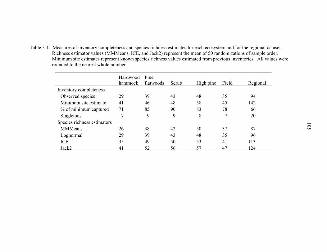
105

Table 3-1. Measures of inventory completeness and species richness estimates for each ecosystem and for the regional dataset. Richness estimator values (MMMeans, ICE, and Jack2) represent the mean of 50 randomizations of sample order. Minimum site estimates represent known species richness values estimated from previous inventories. All values were rounded to the nearest whole number.

Hardwood hammock

Pine flatwoods Scrub High pine Field Regional

Inventory completeness Observed species 29

39 43 48 35 94 Minimum site estimate 41 46 48 58 45 142 % of minimum captured 71 85 90 83 78 66 Singletons 7

9 9 8 7 20

Species richness estimators MMMeans 26 38 42 50 37 87

Lognormal

29 39 43 48 35 96 ICE 35 49 50 53 41 113 Jack2 41 52 56 57 47 124

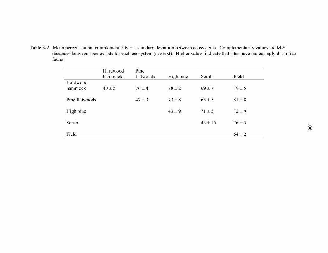
Table 3-2. Mean percent faunal complementarity ± 1 standard deviation between ecosystems. Complementarity values are M-S distances between species lists for each ecosystem (see text). Higher values indicate that sites have increasingly dissimilar fauna.

106

Hardwood hammock

Pine flatwoods High pine Scrub Field

Hardwood hammock 40 ± 5 76 ± 4 78 ± 2 69 ± 8 79 ± 5

Pine flatwoods 47 ± 3 73 ± 8 65 ± 5 81 ± 8

High pine 43 ± 9 71 ± 5 72 ± 9

Scrub 45 ± 15 76 ± 5

Field 64 ± 2

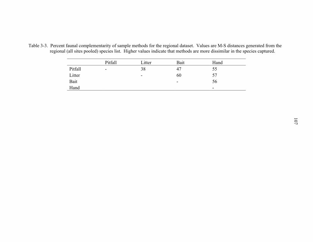
Table 3-3. Percent faunal complementarity of sample methods for the regional dataset. Values are M-S distances generated from the regional (all sites pooled) species list. Higher values indicate that methods are more dissimilar in the species captured.

Pitfall Litter Bait Hand

Pitfall - 38 47 55Litter

- 60 57Bait - 56Hand -

107

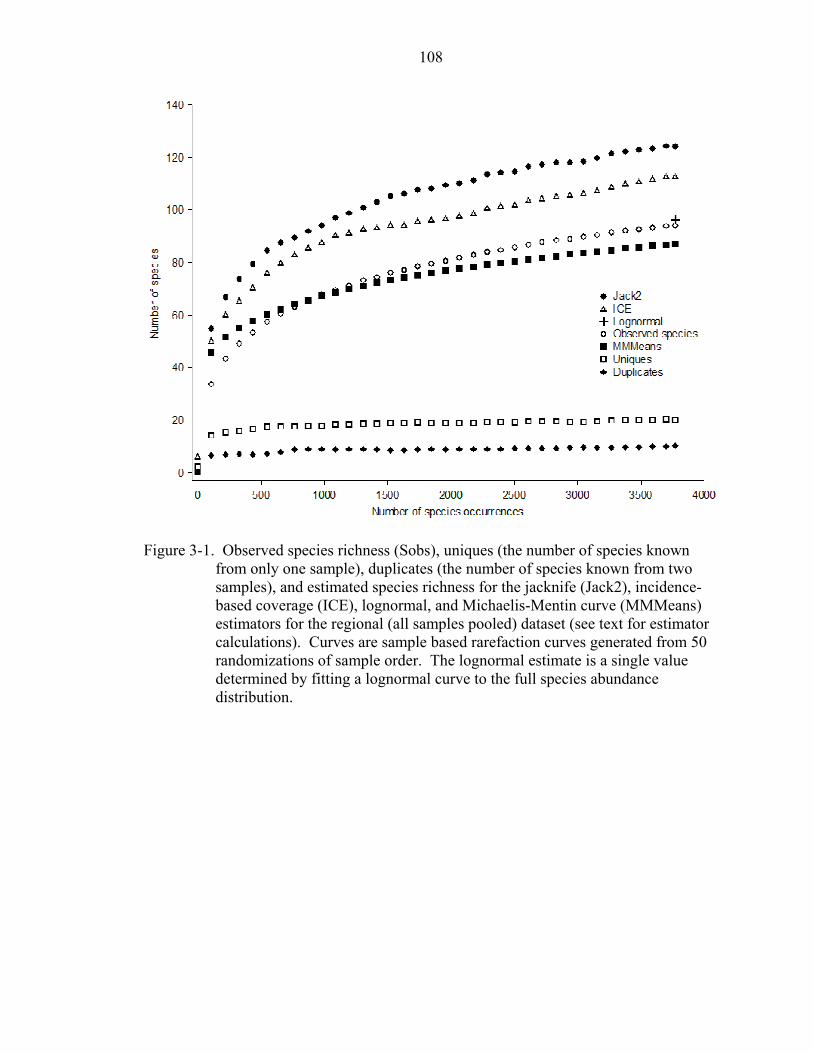
108

Figure 3-1. Observed species richness (Sobs), uniques (the number of species known

from only one sample), duplicates (the number of species known from two samples), and estimated species richness for the jacknife (Jack2), incidence-based coverage (ICE), lognormal, and Michaelis-Mentin curve (MMMeans) estimators for the regional (all samples pooled) dataset (see text for estimator calculations). Curves are sample based rarefaction curves generated from 50 randomizations of sample order. The lognormal estimate is a single value determined by fitting a lognormal curve to the full species abundance distribution.

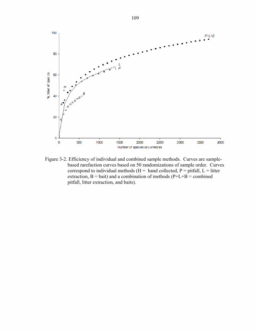
109

Figure 3-2. Efficiency of individual and combined sample methods. Curves are sample-

based rarefaction curves based on 50 randomizations of sample order. Curves correspond to individual methods (H = hand collected, P = pitfall, L = litter extraction, B = bait) and a combination of methods (P+L+B = combined pitfall, litter extraction, and baits).

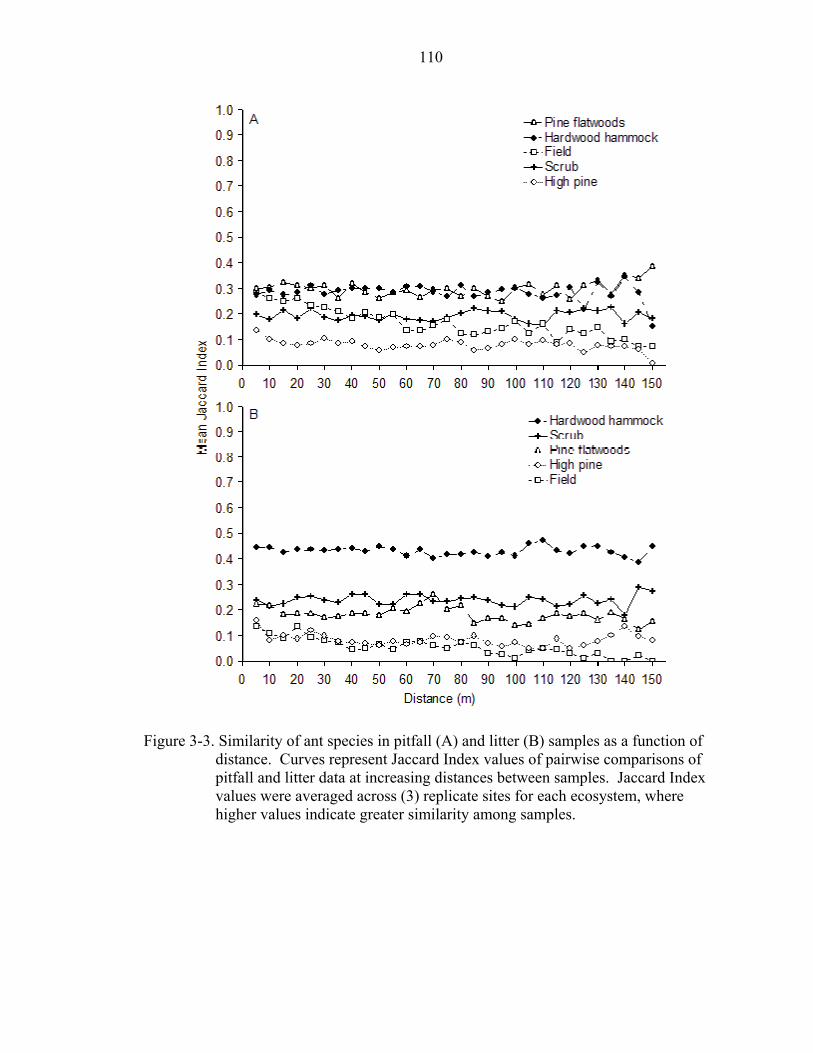
110

Figure 3-3. Similarity of ant species in pitfall (A) and litter (B) samples as a function of

distance. Curves represent Jaccard Index values of pairwise comparisons of pitfall and litter data at increasing distances between samples. Jaccard Index values were averaged across (3) replicate sites for each ecosystem, where higher values indicate greater similarity among samples.

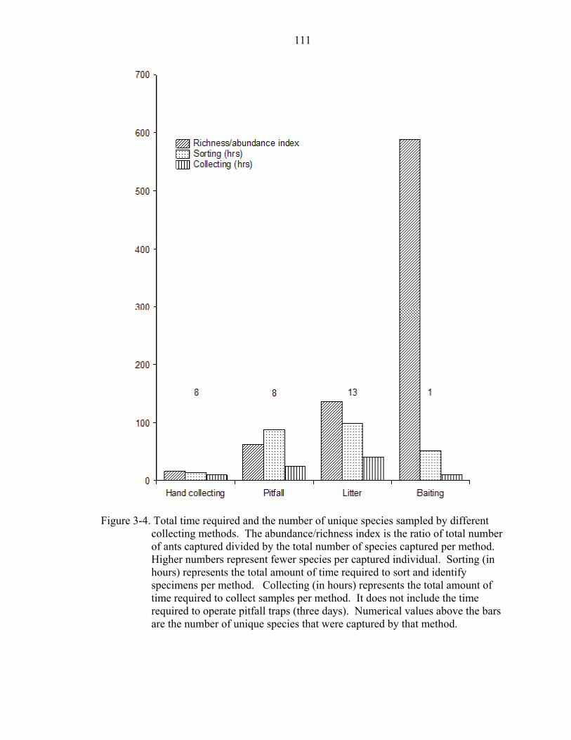
111

Figure 3-4. Total time required and the number of unique species sampled by different

collecting methods. The abundance/richness index is the ratio of total number of ants captured divided by the total number of species captured per method. Higher numbers represent fewer species per captured individual. Sorting (in hours) represents the total amount of time required to sort and identify specimens per method. Collecting (in hours) represents the total amount of time required to collect samples per method. It does not include the time required to operate pitfall traps (three days). Numerical values above the bars are the number of unique species that were captured by that method.

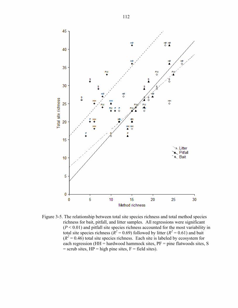
112

Figure 3-5. The relationship between total site species richness and total method species

richness for bait, pitfall, and litter samples. All regressions were significant (P < 0.01) and pitfall site species richness accounted for the most variability in total site species richness (R2 = 0.69) followed by litter (R2 = 0.61) and bait (R2 = 0.46) total site species richness. Each site is labeled by ecosystem for each regression (HH = hardwood hammock sites, PF = pine flatwoods sites, S = scrub sites, HP = high pine sites, F = field sites).

CHAPTER 4 CONCLUSION

Myrmecology is in an exciting phase of its history. Molecular systematics (e.g.

Saux et al. 2004) is providing a much clearer resolution of the phylogeny of ants (Bolton

2003). The fundamental biological processes responsible for ant abundance and diversity

are becoming clearer (Kaspari 2001, Kaspari et al. 2000 a, b, 2003, 2004, Davidson et al.

2003). The natural history of more species is becoming clearer, including a number of

exotic species (e.g. Tschinkel 1993). Finally, sampling methodology is becoming

standardized in a variety of habitats (Agosti et al. 2000a). This study contributes to this

growing field and establishes a data set that is useful for entomologists and

myrmecologists in Florida, the U.S. and the World.

There were three issues that were of principle concern to me throughout my

dissertation research. First, the factors regulating the distribution, diversity, and

abundance of most animals, and insects in particular, are not well understood. This lack

of knowledge leaves a significant gap in our understanding of how terrestrial ecosystems

function and what the immediate and future consequences of environmental change may

be. Empirically-based, quantitative studies of insect community ecology across scales,

although challenging, represent our best chance for quantifying how environmental

change impacts insect communities. These studies should be considered an essential

component of ecosystem research. The first objective of my dissertation research was to

use quantitative, empirically based science to establish the relationship among ant

diversity, abundance, and biomass at local and regional scales. It provides a null model

113

114

for testing alternative hypotheses about other factors structuring insect communities

including competition and resource availability. Additionally, my dissertation research

will serve as a starting point for new research on the role of insects in energy flow and

ecosystem function.

Second, exotic species invasions are among the most important, costly, and

troublesome phenomenon that modern scientists face. Predicting and limiting the spread

of exotic species is predicated on understanding the mechanisms responsible for their

success. Insect invaders are problematical due to our lack of knowledge about the

biology and ecology of most species and their significant impact on ecosystem

functioning. In my study I provided a clearer picture of the distribution, abundance, and

diversity of exotic ant species in native environments in Florida. Results also suggest

that exotic species are constrained by the same factors that constrain native species, and

in some ways may be more ecologically constrained than native species by their apparent

dependence on anthropogenic disturbance to facilitate their spread.

Third, sampling methodology for ants (and insects in general) is by no means

standardized and few data are available to provide guidelines for designing

comprehensive sampling protocol in a variety of habitats outside the tropics. This is a

major impediment to exploring the first and second issues I examined in my dissertation.

The results presented in my dissertation revealed that the sampling issues in temperate

and subtropical ecosystems differ from those in tropical forests, and implementing a

thorough sampling protocol is feasible, if challenging.

Ultimately, the results of my dissertation must be viewed as a starting point. My

study provides one of the most comprehensive examinations of a regional ant fauna, and

115

guidelines for thoroughly sampling warm temperate and subtropical ant assemblages. I

hope that this information will be built upon to further our understanding of ants and

insects. There are numerous questions that remain unanswered, and a number of new

questions have arisen. I am also hopeful that these questions are the beginning of my

personal, career-long cycle of applying the scientific method (observe, hypothesize, test,

analyze, conclude; observe, hypothesize, test, analyze, conclude…). As such, my

dissertation research probably will, at least partially, define my research career.

Regardless, I view this dissertation as a personally fulfilling and successful undertaking if

only because it makes a meaningful contribution to the field of myrmecology.

LIST OF REFERENCES

Abensperg-Traun, M., and D. Steven. 1995. The effects of pitfall trap diameter on ant species richness (Hymenoptera: Formicidae) and species composition of the catch in a semi-arid eucalypt woodland. Australian Journal of Ecology 20: 282-287.

Abrahamson, W.G., and D.C. Hartnett. 1990. Pine flatwoods and dry prairies. Pages 103-149 in Myers, R.L., and J.J. Ewel, editors. Ecosystems of Florida. University of Central Florida Press, Orlando, Florida, USA.

Abrahamson, W.G., A.F. Johnson, J.N. Layne, and P.A. Peroni. 1984. Vegetation of the Archbold Biological Station, Florida: an example of the southern Lake Wales Ridge. Florida Scientist 47: 209-250.

Adams, C.T. 1986. Agricultural and medical impact of the imported fire ants. Pages 48-57 in C.S. Lofgren and R.K. Vander Meer, editors. Fire ants and leaf-cutting ants: biology and management. Westview Press, Boulder, Colorado, USA.

Agosti, D., J.D. Majer, L.E. Alonso, and T.R. Schultz, editors. 2000a. Ants: standard methods for measuring and monitoring biodiversity. Smithsonian Institution Press, Washington D.C., USA.

Agosti, D., J.D. Majer, L.E. Alonso, and T.R. Schultz, editors. 2000b. Sampling ground-dwelling ants: case studies from the world’s rain forests. Curtin University School of Environmental Biology Bulletin No. 18. Perth, Australia.

Andersen, A.N. 1990. The use of ant communities to evaluate change in Australian terrestrial ecosystems: a review and a recipe. Proceedings of the Ecological Society of Australia 16: 347-357.

Andersen, A.N. 1991. Responses of ground-foraging ant communities to three experimental fire regimes in a savanna forest of tropical Australia. Biotropica 23: 575-585.

Andersen, A.N. 1992. Regulation of “momentary” diversity by dominant species in exceptionally rich ant communities of the Australian seasonal tropics. American Naturalist 140: 401-420.

Andersen, A.N. 1993. Ants as indicators of restoration success at a uranium mine in tropical Australia. Restoration Ecology 1: 156-167.

116

117

Andersen, A.N. 1995. A classification of Australian ant communities, based on functional groups which parallel plant life-forms in relation to stress and disturbance. Journal of Biogeography 22: 15-29.

Andersen, A.N. 1997a. Using ants as bioindicators: multiscale issues in ant community ecology. Conservation Ecology 1: 1-8. [Online, URL: <http://www.consecol.org/vol1/iss1/art8>.]

Andersen, A.N. 1997b. Functional groups and patterns of organization in North American ant communities: a comparison with Australia. Journal of Biogeography 24: 433-460.

Andersen, A.N., B.D. Hoffmann, W.J. Müller, and A.D. Griffiths. 2002. Using ants as bioindicators in land management: simplifying assessment of ant community responses. Journal of Applied Ecology 39: 8-17.

Andersen, A.N., and A.D. Patel. 1994. Meat ants as dominant members of Australian ant communities: an experimental test of their influence on the foraging success and forager abundance of other species. Oecologia 98: 15-24.

Anderson, R.S., and J.S. Ashe. 2000. Leaf litter inhabiting beetles as surrogates for establishing priorities for conservation of selected tropical montane cloud forests in Honduras, Central America (Coleoptera; Staphylinidae, Curculionidae). Biodiversity and Conservation 9: 617-653.

Bassett, Y., and R.L. Kitching. 1991. Species number, species abundance and body length of arboreal arthropods associated with an Australian rainforest tree. Ecological Entomology 16: 391-402.

Bestelmeyer, B.T., D. Agosti, L.E. Alonso, C.R.F. Brandão, W.L. Brown Jr., J.H.C. Delabie, and R. Silvestre. 2000. Field techniques for the study of ground-dwelling ants. Pages122-144 in D. Agosti, J.D. Majer, L.E. Alonso, and T.R. Shultz, editors. Ants: standard methods for measuring and monitoring biodiversity. Smithsonian Institution Press, Washington D.C., USA.

Bestelmeyer, B.T., and J.A. Wiens. 1996. The effects of land use on the structure of ground-foraging ant communities in the Argentine chaco. Ecological Applications 6: 1225-1240.

Bolton, B., 2003. Synopsis and Classification of Formicidae. Memoirs of the American Entomological Institute, vol. 71. The American Entomological Institute, Gainesville, Florida, USA.

Brown, J.H., J.F. Gillooly, A.P. Allen, V.M. Savage, and G.B. West. 2004. Toward a metabolic theory of ecology. Ecology 85: 1771–1789.

Brown, J.H., P.A. Marquet, and M.L. Taper. 1993. Evolution of body size: consequences of an energetic definition of fitness. American Naturalist 142: 573-584.

118

Brown, J.H., and B.A. Maurer. 1987. Evolution of species assemblages: effects of energetic constraints and species dynamics on the diversification of the North American avifauna. American Naturalist 130: 1-17.

Brown, J.H., and P.F. Nicoletto. 1991. Spatial scaling of species composition: body masses of North American land mammals. American Naturalist 138: 1478-1512.

Brown, W.L., Jr. 1953. Revisionary studies in the ant tribe Dacetini. American Midland Naturalist 50: 1-137.

Brown, W.L., Jr. 1976. Contributions toward a reclassification of the Formicidae. Part VI. Ponerinae tribe Ponerini, subtribe Odontomachiti. Section A. Introduction, subtribal characters, genus Odontomachus. Studia Entomologica 19: 67-171.

Brown, W.L., Jr., and E.O. Wilson. 1956. Character displacement. Systematic Zoology 5: 49-64.

Burbidge, A.A. 1991. Cost constraints on surveys for nature conservation. Pages 3-6 in C.R. Margules, and M.P. Austin, editors. Nature conservation: cost effective biological surveys and data analysis. CSIRO, Canberra, Australia.

Burnham, K.P., and W.S. Overton. 1978. Estimation of the size of a closed population when capture probabilities vary among animals. Biometrika 65:623-633.

Burnham, K.P., and W.S. Overton. 1979. Robust estimation of population size when capture probabilities vary among animals. Ecology 60:927-936.

Calder, W.A. 1984. Size, function, and life history. Harvard University Press, Cambridge Massachusetts, USA.

Chazdon, R.L., R.K. Colwell, J.S. Denslow, and M.R. Guariguanta. 1998. Statistical methods for estimating species richness of woody regeneration in primary and secondary rain forests of northeastern Costa Rica. Pages 285-309 in F. Dallmeier and J.A. Comiskey, editors. Forest biodiversity research, monitoring, and modeling. Parthenon Publishing Group, Paris, France.

Chew, A.E., and R.M. Chew. 1980. Body size as a determinant of small-scale distributions of ants in evergreen woodland, southeastern Arizona. Insectes Sociaux 27: 189-202.

Chew, R.M., and J. DeVita. 1980. Foraging characteristics of a desert ant assemblage: functional morphology and species separation. Journal of Arid Environments 3: 75-83.

Clench, H.K. 1979. How to make regional lists of butterflies: some thoughts. Journal of the Lepidopterists’ Society 33: 216-231.

119

Cochran, W.G. 1963. Sampling techniques. Second edition. John Wiley & Sons, New York, New York, USA.

Coddington, J.A., C.E. Griswold, D. Silva, E. Peñaranda, and S.F. Larcher. 1991. Designing and testing sampling protocols to estimate biodiversity in tropical ecosystems. Pages 44-60 in E.C. Dudley, editor. The unity of evolutionary biology: proceedings of the fourth international congress of systematic and evolutionary biology. Dioscorides Press, Portland, Oregon, USA.

Colwell, R.K. 2000. EstimateS: statistical estimation of species richness and shared species from samples. Version 6.0. [Online, URL: <http://viceroy.eeb.uconn.edu/estimates>.]

Colwell, R.K., and J.A. Coddington. 1994. Estimating terrestrial biodiversity through extrapolation. Philosophical Transactions of the Royal Society of London, Series B. 345: 101-118.

Creighton, W.S. 1950. The ants of North America. Bulletin of the Museum of Comparative Zoology 104: 1-585.

Damuth, J. 1981. Population density and body size in mammals. Nature 290: 699-700.

Davidson, D.W. 1977. Species diversity and community organization in desert seed-eating ants. Ecology 58: 711-724.

Davidson, D.W. 1978. Size variability in the worker caste of a social insect (Veromessor pergandei Mayr) as a function of the competitive environment. American Naturalist 112: 523-532.

Davidson, D.W., S.C. Cook, R.R. Snelling, and T.H. Chua. 2003. Explaining the abundance of ants in lowland tropical rainforest canopies. Science 300: 969-972.

Delabie, J.H.C., B.L. Fisher, J.D. Majer, and I.W. Wright. 2000. Sampling effort and choice of methods. Pages 145-154 in D. Agosti, J.D. Majer, L.E. Alonso, and T.R. Schultz, editors. Ants: standard methods for measuring and monitoring biodiversity. Smithsonian Institution Press, Washington D.C., USA.

Denno, R.F., M.S. McClure, and J.R. Ott. 1995. Interspecific interactions in phytophagous insects: competition reexamined and resurrected. Annual Review of Entomology 40: 297-331.

Deyrup, M. 2003. An updated list of Florida ants (Hymenoptera: Formicidae). Florida Entomologist 86: 43-48.

Deyrup, M., L. Davis, and S. Cover. 2000. Exotic ants in Florida. Transactions of the American Entomological Society 126: 293-326.

120

Deyrup, M., and J. Trager. 1986. Ants of the Archbold Biological Station, Highlands County, Florida (Hymenoptera: Formicidae). Florida Entomologist 69: 206-228.

Dial, K.P., and J.M. Marzluff. 1988. Are the smallest organisms the most diverse? Ecology 69: 1620-1624.

Diamond, J.M. 1975. Assembly of species communities. Pages 342-444 in M.L. Cody and J.M. Diamond, editors. Ecology and evolution of communities. Harvard University Press, Cambridge, Massachusetts, USA.

Disney, R.H.L. 1986. Assessments using invertebrates: posing the problem. Pages 271-293 in M.B. Usher, editor. Wildlife conservation evaluation. Chapman & Hall, London, UK.

Dobyns, J.R. 1997. Effects of sampling intensity on the collection of spider (Araneae) species and the estimation of spider richness. Environmental Entomology 26: 150-162.

Eldredge, N., editor. 1992. Systematics, ecology, and the biodiversity crisis. Columbia University Press, New York, New York, USA.

Elton, C.S. 1946. Competition and the structure of ecological communities. Journal of Animal Ecology 15: 54-68.

Fisher, B.L. 1996. Ant diversity patterns along an elevational gradient in the Réserve Naturelle Intégrale d’Andringitra, Madagascar. Fieldiana: Zoology 85: 93-108.

Fisher, B.L. 1998. Ant diversity patterns along an elevational gradient in the Réserve Spéciale d’Anjanaharibe-Sud and on the western Masoala Peninsula, Madagascar. Fieldiana: Zoology 90: 39-67.

Fisher, B.L. 1999a. Improving inventory efficiency: a case study of leaf-litter ant diversity in Madagascar. Ecological Applications 9: 714-731.

Fisher, B.L. 1999b. Ant diversity patterns along an elevational gradient in the Réserve Naturelle Intégrale d’Andohahela, Madagascar. Fieldiana: Zoology 94: 129-147.

Fisher, B.L. 2002. Ant diversity patterns along an elevational gradient in the Réserve Spéciale de Manongarivo, Madagascar. Boissiera 59: 311-328.

Fisher, B.L., and H.G. Robertson. 2002. Comparison and origin of forest and grassland ant assemblages in the high plateau of Madagascar (Hymenoptera: Formicidae). Biotropica 34: 155-167.

Floren, A. and K.E. Linsenmair. 2000. Do ant mosaics exist in pristine lowland rain forests? Oecologia 123: 129-137.

121

Folgarait, P.J. 1998. Ant biodiversity and its relationship to ecosystem functioning: a review. Biodiversity and Conservation 7: 1221-1244.

Fowler, H.G. 1980. Populations, prey capture and sharing, and foraging of the Paraguayan Ponerine Odontomachus chelifer Latreille. Journal of Natural History 14: 79-84.

Gholz, H.L., S.A. Vogel, W.P. Cropper, Jr., K. McKelvey, K.C. Ewel, R.O. Teskey, and P.J. Curran. 1991. Dynamics of canopy structure and light interception in Pinus elliottii stands, north Florida. Ecological Monographs 61: 33-51.

Golkin, K.R., and K.C. Ewel. 1984. A computer simulation of the carbon, phosphorus, and hydrologic cycles of a pine flatwoods ecosystem. Ecological Modelling 24: 113-136.

Gotelli, N.J., and A.E. Arnett. 2000. Biogeographic effects of red fire ant invasion. Ecology Letters 3: 257-261.

Gotelli, N.J., and R.K. Colwell. 2001. Quantifying biodiversity: procedures and pitfalls in the measurement and comparison of species richness. Ecology Letters 4: 379-391.

Gotelli, N.J., and A.M. Ellison. 2002a. Biogeography at a regional scale: determinants of ant species density in New England bogs and forests. Ecology 83: 1604-1609.

Gotelli, N.J., and A.M. Ellison. 2002b. Assembly rules for New England ant assemblages. Oikos. 99: 591-599.

Gotelli, N.J., and G.L. Entsminger. 2001. EcoSim: null models software for ecology. Version 7.0. Acquired Intelligence Inc. & Kesey-Bear. [Online, URL: <http://homepages.together.net/~gentsmin/ecosim.htm>.]

Gotelli, N.J., and D.J. McCabe. 2002. Species co-occurrence: a meta-analysis of J.M. Diamond’s assembly rules model. Ecology 83: 2091-2096.

Harrison, S., S.J. Ross, and J.H. Lawton. 1992. Beta diversity on geographic gradients in Britain. Journal of Animal Ecology 61: 151-158.

Herbers, J.M. 1989. Community structure in north temperate ants: temporal and spatial variation. Oecologia 81: 201-211.

Holldöbler, B., and C.J. Lumsden. 1980. Territorial strategies in ants. Science 210: 732-739.

Hölldobler, B., and E.O. Wilson. 1990. The ants. Belknap Press, Cambridge, Massachusetts, USA.

122

Holway, D.A., L. Lach, A.V. Suarez, N.D. Tsutsui, and T.J. Case. 2002. The causes and consequences of ant invasions. Anuual Review of Ecology and Systematics 33: 181-233.

Hubbell, T.H. 1960. Endemism and speciation in relation to Pleistocene changes in Florida and the southeastern coastal plain. Eleventh International Congress of Entomology, Vienna, Austria 1: 466-469.

Hughes, R.G. 1986. Theories and models of species abundance. American Naturalist 128: 879-899.

Huston, M.A. 1979. A general hypothesis of species diversity. American Naturalist 113: 81-101.

Huston, M.A. 1994. Biological diversity: the coexistence of species on changing landscapes. Cambridge University Press, Cambridge, UK.

Hutchinson, G.E. 1959. Homage to Santa Rosalia or why are there so many kinds of animals? American Naturalist 93: 145-159.

Hutchinson, G.E. 1978. An introduction to population ecology. Yale University Press, New Haven, Connecticut, USA.

Hutchinson, G.E., and R.H. MacArthur. 1959. A theoretical ecological model of size distributions among species of animals. American Naturalist 93: 117-125.

Janzen, D.H. 1973. Sweep samples of tropical foliage insects: description of study sites with data on species abundances and size distributions. Ecology 54: 659-686.

Jue, S., C. Kindell, and J. Wojcik. 2001. Florida conservation lands 2001. Florida Natural Areas Inventory, Tallahassee, Florida, USA.

Kaspari, M. 2001. Taxonomic level, trophic biology and the regulation of local abundance. Global Ecology & Biogeography 10: 229-244.

Kaspari, M., L. Alonso, and S. O’Donnell. 2000a. Three energy variables predict ant abundance at a geographical scale. Proceedings of the Royal Society of London, Series B 267: 485-489.

Kaspari, M., S. O’Donnell, and J.R. Kercher. 2000b. Energy, density, and constraints to species richness: ant assemblages along a productivity gradient. American Naturalist 155: 280-293.

Kaspari, M., P.S. Ward, and M. Yuan. 2004. Energy gradients and the geographic distribution of local ant diversity. Oecologia 140: 407-413.

Kaspari, M., and M.D. Weiser. 1999. The size-grain hypothesis and interspecific scaling in ants. Functional Ecology 13: 530-538.

123

Kaspari, M., M. Yuan, L. Alonso. 2003. Spatial grain and the causes of regional diversity gradients in ants. American Naturalist 161: 459-477.

Kim, K.C. 1993. Biodiversity, conservation and inventory: why insects matter. Biodiversity and Conservation 2: 191-214.

King, J.R., A.N. Andersen, and A.D. Cutter. 1998. Ants as bioindicators of habitat disturbance: validation of the functional group model for Australia’s humid tropics. Biodiversity and Conservation 7: 1627-1638.

Krebs, C.J. 1994. Ecology: the experimental analysis of distribution and abundance. HarperCollins College Publishers, New York, New York, USA.

Kremen, C. 1992. Assessing the indicator properties of species assemblages for natural areas monitoring. Ecological Applications 2: 203-217.

Kremen, C. 1994. Biological inventory using target taxa: a case study of the butterflies of Madagascar. Ecological Applications 4: 407-422.

Kremen, C., R.K. Colwell, T.L. Erwin, D.D. Murphy, R.F. Noss, and M.A. Sanjayan. 1993. Terrestrial arthropod assemblages: their use in conservation planning. Conservation Biology 7: 796-808.

Lack, D. 1947. Darwin’s finches. Cambridge University Press, Cambridge, UK.

Laessle, A.M. 1942. The plant communities of the Welaka area with special reference to correlation between soils and vegetational succession. Biological Science Series 4, University of Florida Publication, Gainesville, Florida, USA.

Lambshead, J., and H.M. Platt. 1985. Structural patterns of marine benthic assemblages and their relationships with empirical statistical models. Pages 371-380 in P.E. Gibbs, editor. Proceedings of the 19th European Marine Biology Symposium, Plymouth UK, 1984. Cambridge University Press, Cambridge, UK.

Lawton, J.H., D.E. Bignell, B. Bolton, G.F. Bloemers, P. Eggleton, P.M. Hammond, M. Hodda, R.D. Holt, T.B. Larsen, N.A. Mawdsley, N.E. Stork, D.S. Srivastava, and A.D. Watt. 1998. Biodiversity inventories, indicator taxa and effects of habitat modification in tropical forest. Nature 391: 72-76.

Lee, S.M. and A. Chao. 1994. Estimating population size via sample coverage for closed capture-recapture models. Biometrics 50: 88-97.

Levene, H. 1953. Genetic equilibrium when more than one ecological niche is available. American Naturalist 87: 331-333.

Levings, S.C., and N.R. Franks. Patterns of nest dispersion in a tropical ground ant community. Ecology 63: 338-344.

124

Levings, S.C., and J.F.A. Traniello. 1981. Territoriality, nest dispersion and community structure in ants. Psyche 88: 265-319.

Levings, S.C., and D.M. Windsor. 1984. Litter moisture content as a determinant of litter arthropod distribution and abundance during the dry season on Barro Colorado Island, Panama. Biotropica 16: 125-131.

Lofgren, C.S. 1986. The economic importance and control of imported fire ants in the United States. Pages 227-256 in S.B. Vinson, editor. Economic impact and control of social insects. Praeger, New York, New York, USA.

Longino, J.T. 2000. What to do with the data. Pages 186 – 203 in D. Agosti, J.D. Majer, L.E. Alonso, and T.R. Schultz, editors. Ants: standard methods for measuring and monitoring biodiversity. Smithsonian Institution Press, Washington, D.C., USA.

Longino, J.T., J. Coddington, and R.K. Colwell. 2002. The ant fauna of a tropical rainforest: estimating species richness three different ways. Ecology 83: 689-702.

Longino, J.T., and R.K. Colwell. 1997. Biodiversity assessment using structured inventory: capturing the ant fauna of a tropical rain forest. Ecological Applications 7: 1263-1277.

Lubertazzi D., and W.R. Tschinkel. 2003. Ant community change across a ground vegetation gradient in north Florida's longleaf pine flatwoods. Journal of Insect Science 3:21, 17pp. [Online, url: <http://insectscience.org/3.21>.]

Ludwig, J.A., and J.F. Reynolds. 1988. Statistical ecology: a primer on methods and computing. John Wiley and Sons, New York, New York, USA.

Lugo, A.E., J.F. Gamble, and K.C. Ewel. 1978. Organic matter flows in a mixed-hardwood forest in north central Florida. Pages 790-800. in D. C. Adriano and I. L. Brisbin, Jr., editors. Environmental chemistry and cycling processes. DOE symposium series, CONF-760429.

MacArthur, R.H. 1957. On the relative abundance of bird species. Proceedings of the National Academy of Science, USA 43: 293-295.

MacArthur, R.H., and E.O. Wilson. 1967. The theory of island biogeography. Princeton University Press, Princeton, New Jersey, USA.

Magurran, A.E. 1988. Ecological diversity and its measurement. Princeton University Press, Princeton, New Jersey, USA.

Majer, J.D. 1983. Ants: bio-indicators of minesite rehabilitation, land-use, and land conservation. Environmental Management 7: 375-385.

Majer, J.D. 1997. The use of pitfall traps for sampling ants – a critique. Memoirs of the Museum of Victoria 56: 323-329.

125

Marquet, P.A., S.A. Navarrete, and J.C. Castilla. 1995. Body size, population density, and the energetic equivalence rule. Journal of Animal Ecology 64: 325-332.

Maurer, B.A., and J.H. Brown. 1988. Distribution of energy use and biomass among species of North American terrestrial birds. Ecology 69: 1923-1932.

Maurer, B.A., J.H. Brown, and R.D. Rusler. 1992. The micro and macro in body size evolution. Evolution 46: 939-953.

May, R.M. 1975. Patterns of species abundance and diversity. Pages 81-120 in M.L. Cody and J.M. Diamond, editors. Ecology and evolution of communities. Belknap Press, Cambridge, Massachusetts, USA.

May, R.M. 1978. The dynamics and diversity of insect faunas. Pages 188-204 in L.A. Mound and N. Waloff, editors. Diversity of insect faunas. Blackwell, Oxford, U.K.

McGlynn, T.P. 1999. The worldwide transfer of ants: geographical distribution and ecological invasions. Journal of Biogeography 26: 535-548.

Meffe, G.K., and C.R. Carroll. 1997. Principles of conservation biology. Second edition. Sinauer Associates, Sunderland, Massachusetts, USA.

Megonigal, J.P., W.H. Conner, S. Kroeger, and R.R. Sharitz. 1997. Aboveground production in southeastern floodplain forests: A test of the subsidy-stress hypothesis. Ecology 78:370-384.

Melbourne, B.A. 1999. Bias in the effect of habitat structure on pitfall traps: an experimental evaluation. Australian Journal of Ecology 24: 228-239.

Mitchell, R.J., L.K. Kirkman, S.D. Pecot, C.A. Wilson, B.J. Palik, and L.R. Boring. 1999. Patterns and controls of ecosystem function in longleaf pine – wiregrass savannas. I. Aboveground net primary productivity. Canadian Journal of Forest Research 29: 743-751.

Morrison, L.W. 1996. Community organization in a recently assembled fauna: the case of Polynesian ants. Oecologia 107: 243-256.

Morrison, L.W. 1998. The spatiotemporal dynamics of insular ant metapopulations. Ecology 79: 1135-1146.

Morrison, L.W. 2000. Mechanisms of interspecific competition among an invasive and two native fire ants. Oikos 90: 238-252.

Morrison, L.W. 2002. Long-term impacts of an arthropod-community invasion by the imported fire ant, Solenopsis invicta. Ecology 83: 2337-2345.

126

Morse, D.R., N.E. Stork, and J.H. Lawton. 1988. Species number, species abundance and body length relationships of arboreal beetles in Bornean lowland rain forest trees. Ecological Entomology 13: 25-37.

Myers, R.L. 1990. Scrub and high pine. Pages 150-193 in Myers, R.L., and J.J. Ewel, editors. Ecosystems of Florida. University of Central Florida Press, Orlando, Florida, USA.

Myers, R.L., and J.J. Ewel, editors. 1990a. Ecosystems of Florida. University of Central Florida Press, Orlando, Florida, USA.

Myers, R.L., and J.J. Ewel. 1990b. Problems, prospects, and strategies for conservation. Pages 619-632 in Myers, R.L., and J.J. Ewel, editors. Ecosystems of Florida. University of Central Florida Press, Orlando, Florida, USA.

New, T.R. 1998. Invertebrate surveys for conservation. Oxford University Press, New York, New York, USA.

Odum, E.P. 1960. Organic production and turnover in old field succession. Ecology 41:34-49.

Oliver, I., and A.J. Beattie. 1996. Designing a cost-effective invertebrate survey: a test of methods for rapid assessment of biodiversity. Ecological Applications 6: 594-607.

Paine, R.T. 1974. Intertidal community structure: experimental studies on the relationship between a dominant competitor and its principal predator. Oecologia 15: 93-120.

Peters, R.H. 1983. The ecological implications of body size. Cambridge University Press, Cambridge, U.K.

Pimm, S.L., H.L. Jones, and J. Diamond. 1988. On the risk of extinction. American Naturalist 132: 757-785.

Platnick, N.I. 1992. Patterns of biodiversity. Pages 15-24 in N. Eldredge, editor. Systematics, ecology and the biodiversity crisis. Columbia University Press, New York, New York, USA.

Platt, W.J., and M.W. Schwartz. 1990. Temperate hardwood forests. Pages 194-229 in Myers, R.L., and J.J. Ewel, editors. Ecosystems of Florida. University of Central Florida Press, Orlando, Florida, USA.

Porter, S.D. 1988. Impact of temperature on colony growth and developmental rates of the ant, Solenopsis invicta. Journal of Insect Physiology 34: 1127-1133.

Porter, S.D., and D.A. Savignano. 1990. Invasion of polygyne fire ants decimates native ants and disrupts arthropod community. Ecology 71: 2095-2106.

Preston, F.W. 1948. The commonness and rarity of species. Ecology 29: 254-283.

127

Preston, F.W. 1962. The canonical distribution of commonness and rarity. 1. Ecology 43: 410-432.

Price, P.W. 1997. Insect ecology. John Wiley & Sons, New York, New York, USA.

Price, P.W. and G.P. Waldbauer. 1994. Ecological aspects of pest management. Pages 35-72 in R.L. Metcalf and W.H. Luckmann, editors. Introduction to insect pest management. John Wiley & Sons, New York, New York, USA.

Prusack, Z.A. 1997. Ant fauna in three plant communities within Wekiwa Springs State Park, Florida: assessment of diversity and comparison of collecting methods. Unpublished Master’s thesis. University of Central Florida.

Raaijmakers, J.G.W. 1987. Statistical analysis of the Michaelis-Menten equation. Biometrics 43:793-803.

Rabinowitz, D. 1981. Seven forms of rarity. Pages 205-217 in H. Synge, editor. The biological aspects of rare plant conservation. Wiley, New York, New York, USA.

Rabinowitz, D., S. Cairns, and T. Dillon. 1986. Seven forms of rarity and their frequency in the flora of the British Isles. Pages 182-204 in M. Soulé, editor. Conservation biology, the science of scarcity and diversity. Sinauer Associates, Sunderland, Massachusetts, USA.

Raven, P.H., and E.O. Wilson. 1992. A fifty-year plan for biodiversity surveys. Science 258: 1099-1100.

Rees, K., A. Buckling, G. Bell, and P.B. Rainey. 2000. Diversity peaks at intermediate productivity in a laboratory microcosm. Nature 406: 508-512.

Ribas, C.R. and J.H. Schoereder. 2002. Are all ant mosaics caused by competition? Oecologia 131: 606-611.

Ricklefs, R.E., and D. Schluter, editors. 1993. Species diversity in ecological communities. University of Chicago Press, Chicago, USA.

Rogers, L.E., W.T. Hinds, and R.L. Buschbom. 1976. A general weight vs. length relationship for insects. Annals of the Entomological Society of America 69: 387-389.

Root, R.B. 1973. Organization of a plant-arthropod association in simple and diverse habitats: the fauna of collards (Brassica oleracea). Ecological Monographs 43: 96-124.

Rosenzweig, R.L. 1995. Species diversity in space and time. Cambridge University Press, Cambridge, UK.

128

Rosenzweig, M.L., and Z. Abramsky. 1993. How are diversity and productivity related? Pages 52-65 in R.E. Ricklefs and D. Schluter, editors. Species diversity in ecological communities: historical and geographical perspectives. University of Chicago Press, Chicago, Illinois, USA.

Ryti, R.T., and T.J. Case. 1984. Spatial arrangement and diet overlap between colonies of desert ants. Oecologia 62: 401-404.

Ryti, R.T., and T.J. Case. 1986. Overdispersion of ant colonies: a test of hypotheses. Oecologia 69: 446-453.

Sanders, N.J., N.J. Gotelli, N.E. Heller, and D.M. Gordon. 2003. Community disassembly by an invasive species. Proceedings of the National Academy of Sciences, USA 100: 2474-2477.

Saux, C., B.L. Fisher, and G.S. Spicer. 2004. Dracula ant phylogeny as inferred by nuclear 28S rDNA sequences and implications for ant systematics (Hymenoptera: Formicidae: Amblyoponinae). Molecular Phylogenetics and Evolution 33: 457-468.

Savage, V.M., J.F. Gillooly, J.H. Brown, G.B. West, and E.L. Charnov. 2004. Effects of body size and temperature on population growth. American Naturalist 163: 429-441.

Schmalzer, P.A., and C.R. Hinkle. 1996. Biomass and nutrients in aboveground vegetation and soils of Florida oak-saw palmetto scrub. Castanea 61: 168-193.

Schortemeyer, M., P. Dijkstra, D.W. Johnson, and B.G. Drake. 2000. Effects of elevated atmospheric CO2 concentration on C and N pools and rhizosphere processes in a Florida scrub oak community. Global Change Biology 6: 383-391.

Siemann, E., D. Tilman and J. Haarstad. 1996. Insect species diversity, abundance and body size relationships. Nature 380: 704-706.

Siemann, E., D. Tilman, and J. Haarstad. 1999. Abundance, diversity and body size: patterns from a grassland arthropod community. Journal of Animal Ecology 68: 824-835.

Silva, D., and J.A. Coddington. 1996. Spiders of Pakitza (Madre de Dios) Peru: species richness and notes on community structure. Pages 241-299 in D.E. Wilson, and A. Sandoval, editors. The biodiversity of Pakitza and its environs. Smithsonian Institution, Washington, D.C., USA.

Simberloff, D. 1983. Sizes of coexisting species. Pages 404-430 in D.J. Futuyma and M. Slatkin, editors. Coevolution. Sinaur Associates, Sunderland, Massachusetts, USA.

Soberón, J.M., and J. Llorente. 1993. The use of species accumulation functions for the prediction of species richness. Conservation Biology 7: 480-488.

129

Sørensen, L.L., J.A. Coddington, and N. Scharff. 2002. Inventorying and estimating subcanopy spider diversity using semiquantitative sampling methods in an Afromontane forest. Environmental Entomology 31: 319-330.

Southwood, T.R.E., and P.A. Henderson. 2000. Ecological methods. Blackwell Science, Malden, Massachussetts, USA.

Stone, L., and A. Roberts. 1990. The checkerboard score and species distributions. Oecologia 85: 74-79.

Stork, N.E., and T.M. Blackburn. 1993. Abundance, body size and biomass of arthropods in tropical forest. Oikos 67: 483-489.

Strayer, D. 1986. The size structure of a lacustrine zoobenthic community. Oecologia 69: 513-515.

Suarez, A.V., D.T. Bolger, and T.J. Case. 1998. Effects of fragmentation and invasion on native ant communities in coastal southern California. Ecology 79: 2041-2056.

Talbot, M. 1975. A list of the ants (Hymenoptera: Formicidae) of the Edwin S. George Reserve, Livingston County, Michigan. Great Lakes Entomologist 8: 245-246.

Tennant, L.E., and S.D. Porter. 1991. Comparison of diets of two fire ant species (Hymenoptera: Formicidae): solid and liquid components. Journal of Entomological Science 26: 450-465.

Thompson, C.R. 1989. The thief ants, Solenopsis molesta group, of Florida (Hymenoptera Formicidae). Florida Entomologist 72: 268-283.

Tilman, D, J. HilleRisLambers, S. Harpole, R. Dybzinski, J. Fargione, C. Clark, and C. Lehman. 2004. Does metabolic theory apply to community ecology? It’s a matter of scale. Ecology 85: 1797-1799.

Tobin, J.E. 1994. Ants as primary consumers: diet and abundance in the Formicidae. Pages 279-307 in J.H. Hunt and C.A. Nalepa, editors. Nourishment and evolution in insect societies. Westview Press, Boulder, Colorado, USA.

Toti, D.S., F.A. Coyle, and J.A. Miller. 2000. A structured inventory of Appalachian grass bald and heath bald spider assemblages and a test of species richness estimator performance. Journal of Arachnology 28: 329-345.

Tschinkel, W.R. 1987. The fire ant, Solenopsis invicta, as a successful “weed.” Pages 585-588 in J. Eder and H. Rembold, editors. Chemistry and biology of social insects. Verlag J. Peperny, München, Germany.

Tschinkel, W.R. 1988. Distribution of the fire ants, Solenopsis invicta and S. geminata in northern Florida in relation to habitat and disturbance. Annals of the Entomological Society of America 81: 76-81.

130

Tschinkel, W.R. 1993. Sociometry and sociogenesis of colonies of the fire ant Solenopsis invicta during one annual cycle. Ecological Monographs 63: 425-457.

Van Pelt, A.F. 1947. Ants of the Gainesville region: with special reference to ecology and taxonomy. Unpublished dissertation. University of Florida.

Van Pelt, A.F. 1956. The ecology of the ants of the Welaka Reserve, Florida. American Midland Naturalist 56: 358-387.

Van Pelt, A.F. 1958. The ecology of the ants of the Welaka Reserve, Florida (Hymenoptera: Formicidae). Part II. Annotated list. American Midland Naturalist 59: 1-57.

Vepsäläinen, K., and B. Pisarski. 1982. Assembly of island ant communities. Annales Zoologici Fennici 19: 327-335.

Vinson, S.B. 1994. Impact of the invasion of Solenopsis invicta (Buren) on native food webs. Pages 240-258 in D.F. Williams, editor. Exotic ants: biology, impact, and control of introduced species. Westview Press, San Francisco, USA.

Wagner, T.L., H. Wu, P.J.H. Sharpe, R.M. Schoolfield, and R.N. Coulson. 1984. Modeling insect development rates: a literature review and applications of a biophysical model. Annals of the Entomological Society of America 77: 208-255.

Webb, S.D. 1990. Historical biogeography. Pages 70-100 in Myers, R.L., and J.J. Ewel, editors. Ecosystems of Florida. University of Central Florida Press, Orlando, Florida, USA.

Whitford, W.G. 1978. Structure and seasonal activity of Chihuahua desert ant communities. Insectes Sociaux 25: 79-88.

Whittaker, R.H. 1975. Communities and ecosystems. Second edition. MacMillan, New York, New York, USA.

Wilson, E.O. 1959. Adaptive shift and dispersal in a tropical ant fauna. Evolution 13: 122-144.

Wilson, E.O. 1961. The nature of the taxon cycle in the Melanesian ant fauna. American Naturalist 95: 169-193.

Wilson, E.O. 1971. The insect societies. Belknap Press, Cambridge, Massachusetts, USA.

Wilson, E.O. 1987. The little things that run the world (The importance and conservation of invertebrates). Conservation Biology 1: 344-346.

Wilson, E.O., editor. 1988. Biodiversity. National Academy Press, Washington, D.C., USA.

131

Wilson, E.O. 2003. Pheidole in the New World: a dominant, hyperdiverse ant genus. Harvard University Press, Cambridge, Massachusetts, USA.

Wilson, J.B. 1999. Assembly rules in plant communities. Pages 130-164 in Weiher, E., and P. Keddy, editors. Ecological assembly rules: perspectives, advances, retreats. Cambridge University Press, Cambridge, UK.

BIOGRAPHICAL SKETCH

Joshua R. King was born in 1974 in Bangor, Maine. He earned a B.S. in biology

from Tufts University (Medford, Massachusetts) in 1997. He earned an M.A. in

education from Tufts University in 1998. His hobbies include animal husbandry,

taxidermy, goat roping, and chainsaw juggling. When he is not contemplating the

mysteries of the universe in his mountain lair in Slaviastav, Siberia, he can be found

collecting ants somewhere in Florida.

132