Another CombinatorialOperator in APL

Bob SmithSudley Place Software

Originally Written24 Aug 2016

Updated29 Sep 2016

Table of ContentsIntroductionTwelvefold WayFunction SelectorSyntaxArgumentsLabeled vs. UnlabeledCounting Partitions of a SetCounting Partitions of a NumberThe Twelve AlgorithmsCase 000 Case 00 1 Case 00 2Case 0 1 0 Case 0 11 Case 0 12Case 1 00 Case 1 0 1 Case 1 0 2Case 11 0 Case 111 Case 112

Summary of Related AlgorithmsSimilarities in The FS TableImplementing the AlgorithmsOpen QuestionsComparing Operator v. FunctionFuture WorkConclusionsOnline VersionReferences

IntroductionCounting and generating items is fundamental in mathematics, but hasbeen sorely lacking in APL (notwithstanding !R and L!R); instead we have had to rely upon a patchwork of various library routines.

Moreover, most APL papers on the topic have focused on the

-1-

implementation of the algorithms rather than their organization and syntax mostly because, at the time, there was no unifying concept.

The main purpose of this paper is to present in APL a unified organizing principle to classify and access these algorithms.

A secondary purpose is to shed light on the relationships between the various algorithms through a new perspective provided by Gian-Carlo Rota’s clever way to fit them into a single organizational framework.

The goal of this paper is to describe a single APL primitive to both count and generate various combinatorial arrays: permutations, combinations, compositions, partitions, etc. The unifying (and very APL-like) principle for such a primitive is Gian-Carlo Rota's TwelvefoldWay as described in Richard Stanley's "Enumerative Combinatorics"1, Knuth’s TAOCP, Vol. 4A3, and Wikipedia2 among other references.

Twelvefold WayThe Twelvefold Way consolidates twelve of these algorithms into a single 2×2×3 array based on the simple concept of placing balls into boxes (urns, to you old-timers). The three dimensions of the array can be described as follows:

● The balls may be labeled (or not) {2 ways},● The boxes may be labeled (or not) {2 ways}, and● The # balls allowed in a box may be one of (at most one |

unrestricted | at least one) {3 ways}.

Amazingly, these twelve choices spanning three dimensions knit together within a single concept (balls in boxes) all of the following interesting, fundamental, and previously disparate and disorganized combinatorial algorithms:

-2-

● Permutations● Combinations● Compositions● Partitions of a set● Partitions of a number● Multisets● Tuples

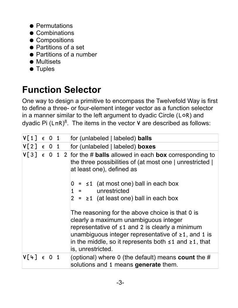
Function SelectorOne way to design a primitive to encompass the Twelvefold Way is firstto define a three- or four-element integer vector as a function selector in a manner similar to the left argument to dyadic Circle (L○R) and dyadic Pi (LπR)8. The items in the vector V are described as follows:

V[1] ∊ 0 1 for (unlabeled | labeled) ballsV[2] ∊ 0 1 for (unlabeled | labeled) boxesV[3] ∊ 0 1 2 for the # balls allowed in each box corresponding to

the three possibilities of (at most one | unrestricted | at least one), defined as

0 = ≤1 (at most one) ball in each box1 = unrestricted2 = ≥1 (at least one) ball in each box

The reasoning for the above choice is that 0 is clearly a maximum unambiguous integer representative of ≤1 and 2 is clearly a minimum unambiguous integer representative of ≥1, and 1 is in the middle, so it represents both ≤1 and ≥1, that is, unrestricted.

V[4] ∊ 0 1 (optional) where 0 (the default) means count the # solutions and 1 means generate them.

-3-

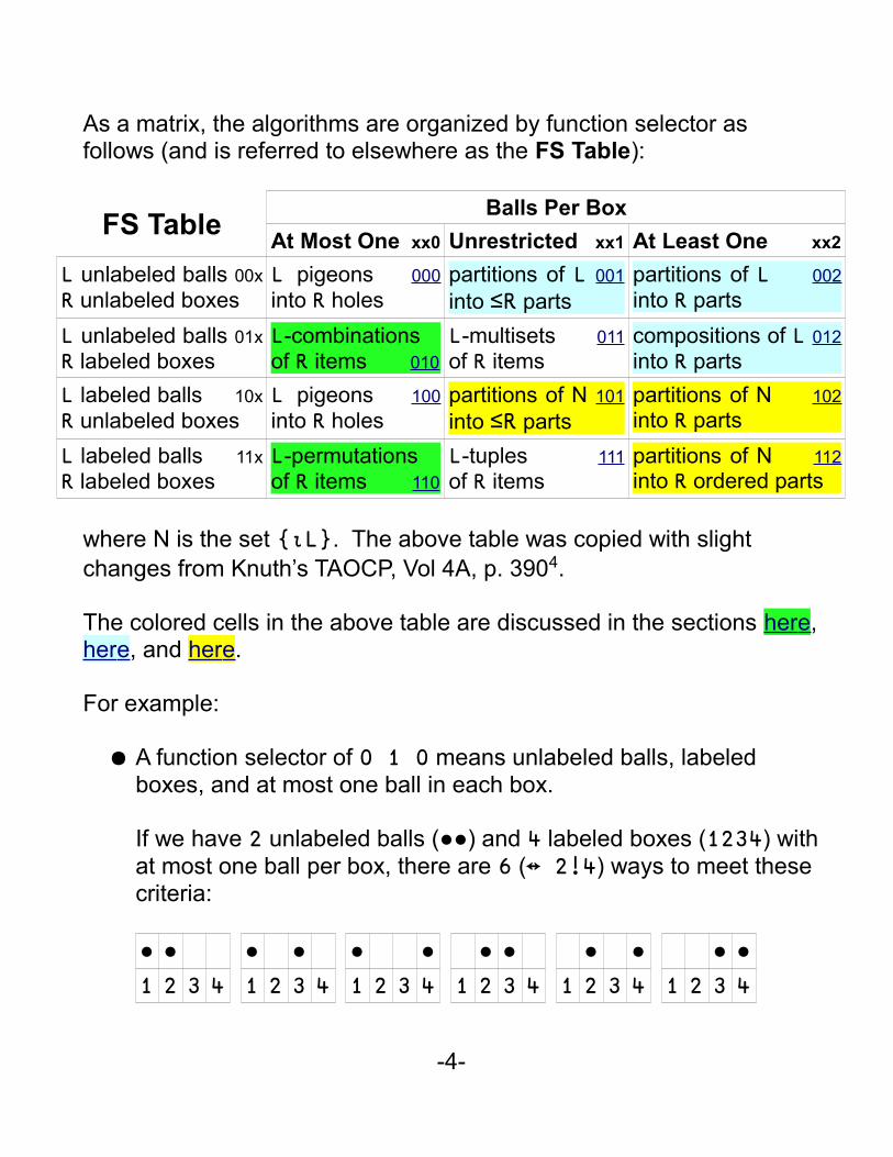
As a matrix, the algorithms are organized by function selector as follows (and is referred to elsewhere as the FS Table):

FS TableBalls Per Box

At Most One xx0 Unrestricted xx1 At Least One xx2

L unlabeled balls 00x

R unlabeled boxesL pigeons 000

into R holespartitions of L 001

into ≤R partspartitions of L 002

into R parts

L unlabeled balls 01x

R labeled boxesL-combinationsof R items 010

L-multisets 011

of R itemscompositions of L 012

into R parts

L labeled balls 10x

R unlabeled boxesL pigeons 100

into R holespartitions of N 101

into ≤R partspartitions of N 102

into R parts

L labeled balls 11x

R labeled boxesL-permutations of R items 110

L-tuples 111

of R itemspartitions of N 112

into R ordered parts

where N is the set {⍳L}. The above table was copied with slight changes from Knuth’s TAOCP, Vol 4A, p. 3904.

The colored cells in the above table are discussed in the sections her e,her e, and her e.

For example:

● A function selector of 0 1 0 means unlabeled balls, labeled boxes, and at most one ball in each box.

If we have 2 unlabeled balls (●●) and 4 labeled boxes (1234) withat most one ball per box, there are 6 (↔ 2!4) ways to meet these criteria:

● ●1 2 3 4

● ●1 2 3 4

● ●1 2 3 4

● ●1 2 3 4

● ●1 2 3 4

● ●1 2 3 4

-4-

from which it is easy to see that these criteria correspond to L combinations of R items (↔ L!R). See case 010 below.

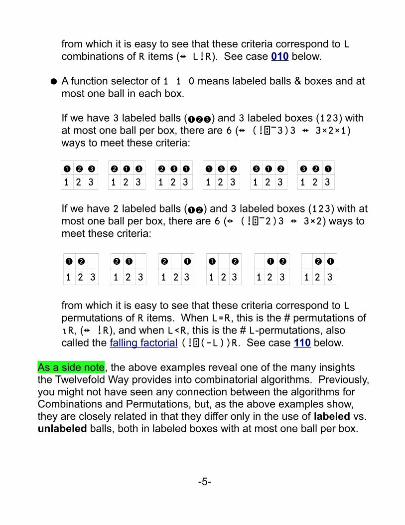
● A function selector of 1 1 0 means labeled balls & boxes and at most one ball in each box.

If we have 3 labeled balls (❶❷❸) and 3 labeled boxes (123) with at most one ball per box, there are 6 (↔ (!⍠¯3)3 ↔ 3×2×1) ways to meet these criteria:

❶ ❷ ❸

1 2 3❷ ❶ ❸

1 2 3❷ ❸ ❶

1 2 3❶ ❸ ❷

1 2 3❸ ❶ ❷

1 2 3❸ ❷ ❶

1 2 3

If we have 2 labeled balls (❶❷) and 3 labeled boxes (123) with at most one ball per box, there are 6 (↔ (!⍠¯2)3 ↔ 3×2) ways to meet these criteria:

❶ ❷

1 2 3

❷ ❶

1 2 3

❷ ❶

1 2 3

❶ ❷

1 2 3

❶ ❷

1 2 3

❷ ❶

1 2 3

from which it is easy to see that these criteria correspond to L permutations of R items. When L=R, this is the # permutations of ⍳R, (↔ !R), and when L<R, this is the # L-permutations, also called the falling factorial (!⍠(-L))R. See case 110 below.

As a side note, the above examples reveal one of the many insights the Twelvefold Way provides into combinatorial algorithms. Previously,you might not have seen any connection between the algorithms for Combinations and Permutations, but, as the above examples show, they are closely related in that they differ only in the use of labeled vs. unlabeled balls, both in labeled boxes with at most one ball per box.

-5-

SyntaxOne way of defining the syntax for such a combinatorial primitive is as a monadic operator (say, the Greek letter lowercase beta β) deriving a dyadic function whose left & right arguments are the # balls & boxes and whose operand is the function selector: L (Vβ) R.

The derived function from the operator is dyadic only and is mixed (i.e.,not scalar). When generating, some of the results are sensitive to ⎕IO,and some generated results may be nested as not all items need be of the same rank and shape.

ArgumentsThe left and right arguments are limited to non-negative integer scalars. Various combinatorial algorithms have been extended to otherdatatypes (e.g., Hypercomplex numbers9), but I’ve chosen not to do that for the initial design.

Labeled vs. UnlabeledBoxes

For most cases, the boxes are the columns of the result. Two or more labeled boxes may hold identical content, but because the boxes are labeled, they are considered distinct. Contrary to the labeled case, unlabeled boxes with identical content are indistinguishable.

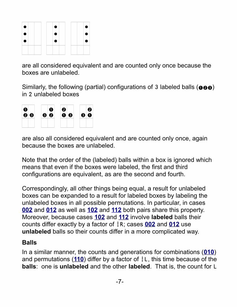
For example, the following (partial) configurations of 3 unlabeled balls (●●●) in 3 unlabeled boxes

-6-

●●●

●●●

●●●

are all considered equivalent and are counted only once because the boxes are unlabeled.

Similarly, the following (partial) configurations of 3 labeled balls (❶❷❸) in 2 unlabeled boxes

❶❷ ❸ ❸

❶❷

❷❶ ❸ ❸

❷❶

are also all considered equivalent and are counted only once, again because the boxes are unlabeled.

Note that the order of the (labeled) balls within a box is ignored which means that even if the boxes were labeled, the first and third configurations are equivalent, as are the second and fourth.

Correspondingly, all other things being equal, a result for unlabeled boxes can be expanded to a result for labeled boxes by labeling the unlabeled boxes in all possible permutations. In particular, in cases 002 and 012 as well as 102 and 112 both pairs share this property. Moreover, because cases 102 and 112 involve labeled balls their counts differ exactly by a factor of !R; cases 002 and 012 use unlabeled balls so their counts differ in a more complicated way.

Balls

In a similar manner, the counts and generations for combinations (010)and permutations (110) differ by a factor of !L, this time because of theballs: one is unlabeled and the other labeled. That is, the count for L

-7-

combinations of R items is

L!R ↔ (!R)÷(!R-L)×!L

and the count for L permutations of R items is

(!⍠(-L)) R ↔ (!R)÷!R-L

Of course, when L=R, the permutation count is the familiar !R.

See the examples above on the differences between labeled and unlabeled balls.

Finally, the generations of the two are related as follows:

a←L (0 1 0 1β) R L combinations of R itemsb←L (1 1 0 1β) L L permutations of L items (L=R)c←L (1 1 0 1β) R L permutations of R items (L<R) c≡,[⎕IO+0 1] a[;b]

Counting Partitions of a SetThe counts in three of the cases below (101, 102, and 112) are dependent on the Stirling numbers of the 2nd kind. They satisfy the following recurrence relation defined on n≥0 and k≥0:

S(0,0) = 1 S(n,k) = k × S(n-1,k) + S(n-1,k-1)

and, for the purposes of this paper, is implemented in the dyadic APL function SN2. These numbers are used in the field of combinatorics and the study of partitions of a set5.

As a side note, as the count for case 102 (the # of partitions of the set

-8-

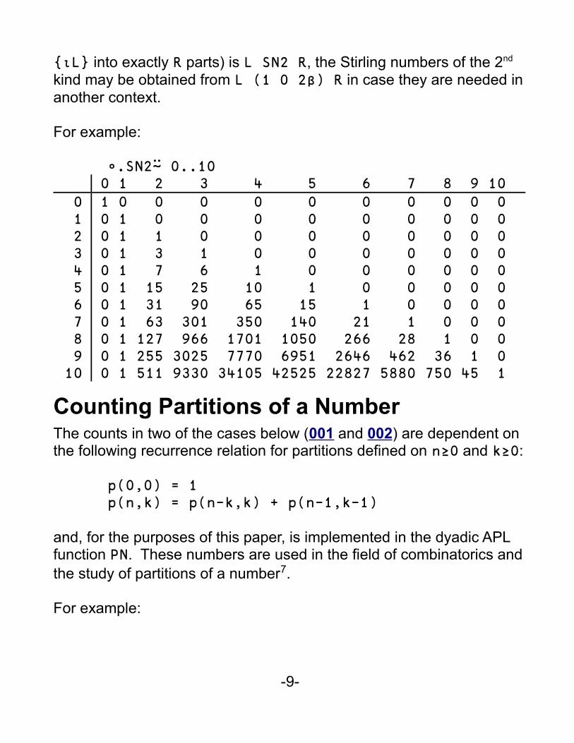
{⍳L} into exactly R parts) is L SN2 R, the Stirling numbers of the 2nd kind may be obtained from L (1 0 2β) R in case they are needed inanother context.

For example:

∘.SN2⍨ 0..10 0 1 2 3 4 5 6 7 8 9 10

0 1 2 3 4 5 6 7 8 9 10

1 0 0 0 0 0 0 0 0 0 0 0 1 0 0 0 0 0 0 0 0 0 0 1 1 0 0 0 0 0 0 0 0 0 1 3 1 0 0 0 0 0 0 0 0 1 7 6 1 0 0 0 0 0 0 0 1 15 25 10 1 0 0 0 0 0 0 1 31 90 65 15 1 0 0 0 0 0 1 63 301 350 140 21 1 0 0 0 0 1 127 966 1701 1050 266 28 1 0 0 0 1 255 3025 7770 6951 2646 462 36 1 0 0 1 511 9330 34105 42525 22827 5880 750 45 1

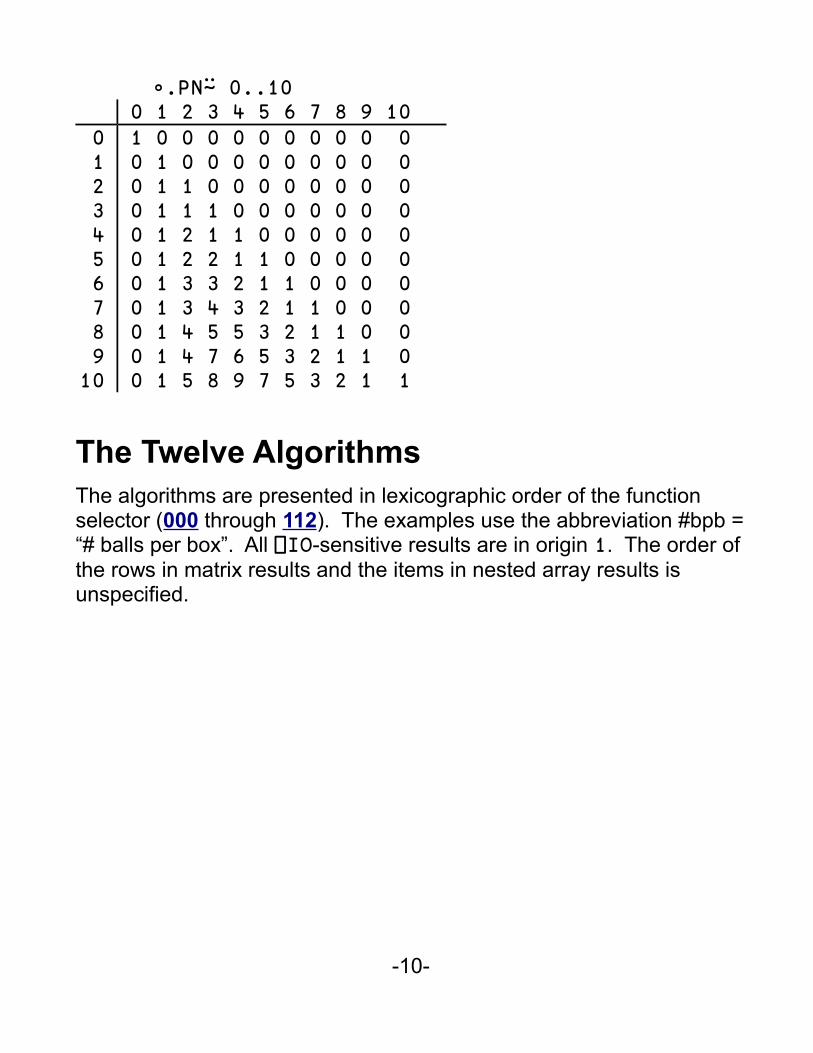
Counting Partitions of a NumberThe counts in two of the cases below (001 and 002) are dependent on the following recurrence relation for partitions defined on n≥0 and k≥0:

p(0,0) = 1 p(n,k) = p(n-k,k) + p(n-1,k-1)

and, for the purposes of this paper, is implemented in the dyadic APL function PN. These numbers are used in the field of combinatorics andthe study of partitions of a number7.

For example:

-9-

∘.PN⍨ 0..10 0 1 2 3 4 5 6 7 8 9 10

0 1 2 3 4 5 6 7 8 9 10

1 0 0 0 0 0 0 0 0 0 0 0 1 0 0 0 0 0 0 0 0 0 0 1 1 0 0 0 0 0 0 0 0 0 1 1 1 0 0 0 0 0 0 0 0 1 2 1 1 0 0 0 0 0 0 0 1 2 2 1 1 0 0 0 0 0 0 1 3 3 2 1 1 0 0 0 0 0 1 3 4 3 2 1 1 0 0 0 0 1 4 5 5 3 2 1 1 0 0 0 1 4 7 6 5 3 2 1 1 0 0 1 5 8 9 7 5 3 2 1 1

The Twelve AlgorithmsThe algorithms are presented in lexicographic order of the function selector (000 through 112). The examples use the abbreviation #bpb =“# balls per box”. All ⎕IO-sensitive results are in origin 1. The order of the rows in matrix results and the items in nested array results is unspecified.

-10-

Case 000: (Back to FS T able)

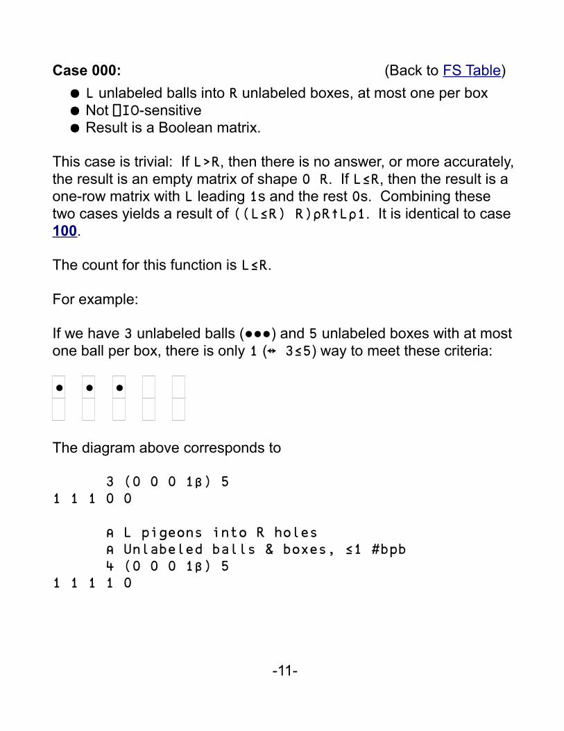
● L unlabeled balls into R unlabeled boxes, at most one per box● Not ⎕IO-sensitive● Result is a Boolean matrix.

This case is trivial: If L>R, then there is no answer, or more accurately,the result is an empty matrix of shape 0 R. If L≤R, then the result is a one-row matrix with L leading 1s and the rest 0s. Combining these two cases yields a result of ((L≤R) R)⍴R↑L⍴1. It is identical to case 100.

The count for this function is L≤R.

For example:

If we have 3 unlabeled balls (●●●) and 5 unlabeled boxes with at most one ball per box, there is only 1 (↔ 3≤5) way to meet these criteria:

● ● ●

The diagram above corresponds to

3 (0 0 0 1β) 51 1 1 0 0

⍝ L pigeons into R holes ⍝ Unlabeled balls & boxes, ≤1 #bpb 4 (0 0 0 1β) 51 1 1 1 0

-11-

Case 001: (Back to FS T able)

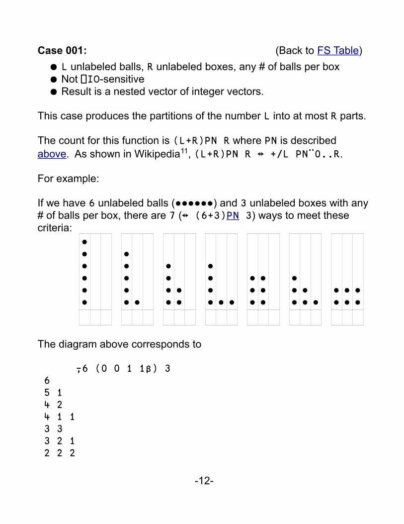
● L unlabeled balls, R unlabeled boxes, any # of balls per box● Not ⎕IO-sensitive● Result is a nested vector of integer vectors.

This case produces the partitions of the number L into at most R parts.

The count for this function is (L+R)PN R where PN is described above. As shown in Wikipedia11, (L+R)PN R ↔ +/L PN¨0..R.

For example:

If we have 6 unlabeled balls (●●●●●●) and 3 unlabeled boxes with any# of balls per box, there are 7 (↔ (6+3)PN 3) ways to meet these criteria:

●●●●●●

●●●●● ●

●●●●●●

●●●● ● ●

●●●

●●●

●●●●● ●

●●●●●●

The diagram above corresponds to

⍪6 (0 0 1 1β) 3 6 5 1 4 2 4 1 1 3 3 3 2 1 2 2 2

-12-

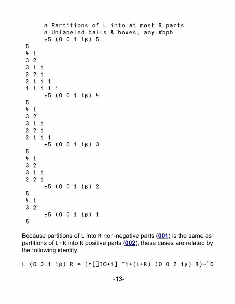
⍝ Partitions of L into at most R parts ⍝ Unlabeled balls & boxes, any #bpb ⍪5 (0 0 1 1β) 5 5 4 1 3 2 3 1 1 2 2 1 2 1 1 1 1 1 1 1 1 ⍪5 (0 0 1 1β) 4 5 4 1 3 2 3 1 1 2 2 1 2 1 1 1 ⍪5 (0 0 1 1β) 3 5 4 1 3 2 3 1 1 2 2 1 ⍪5 (0 0 1 1β) 2 5 4 1 3 2 ⍪5 (0 0 1 1β) 1 5

Because partitions of L into R non-negative parts (001) is the same as partitions of L+R into R positive parts (002), these cases are related by the following identity:

L (0 0 1 1β) R ↔ (⊂[⎕IO+1] ¯1+(L+R) (0 0 2 1β) R)~¨0

-13-

Case 002: (Back to FS T able)

● L unlabeled balls, R unlabeled boxes, at least one ball per box● Not ⎕IO-sensitive● Result is an integer matrix.

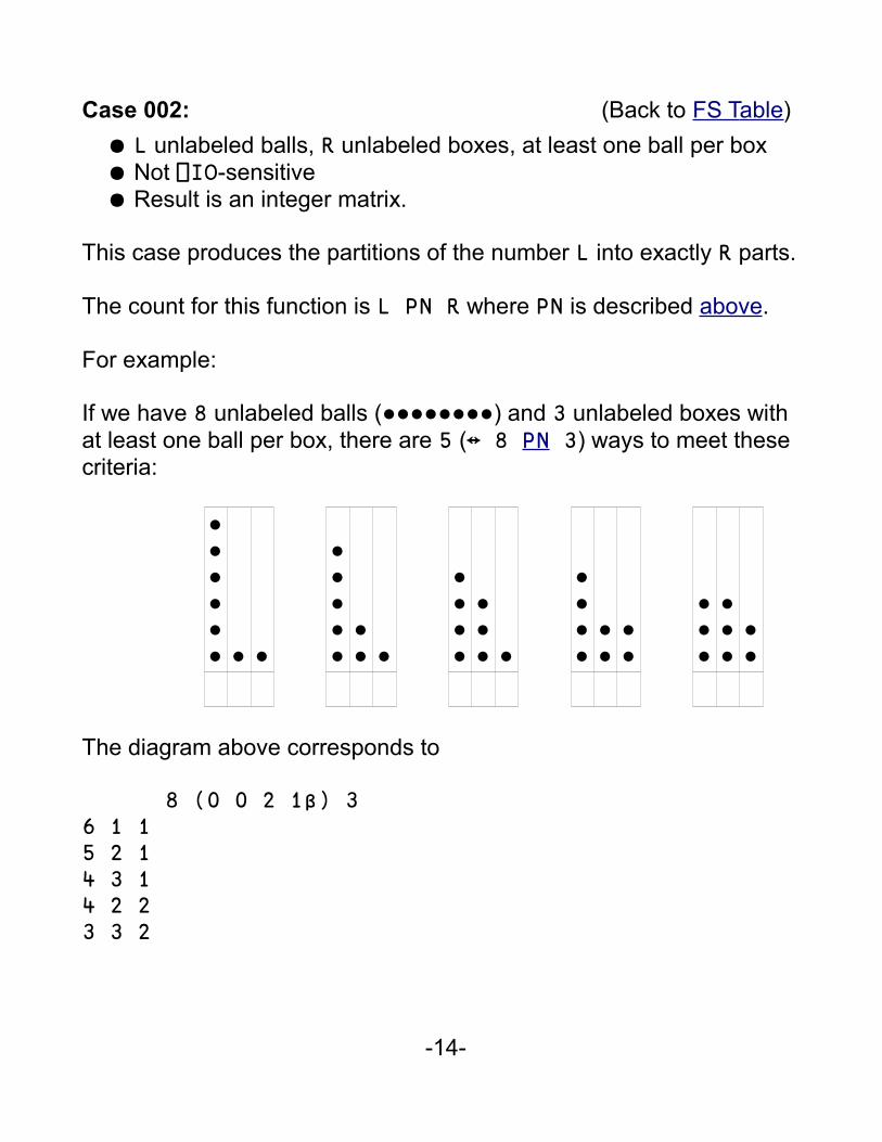
This case produces the partitions of the number L into exactly R parts.

The count for this function is L PN R where PN is described above.

For example:

If we have 8 unlabeled balls (●●●●●●●●) and 3 unlabeled boxes with at least one ball per box, there are 5 (↔ 8 PN 3) ways to meet these criteria:

●●●●●● ● ●

●●●●●●● ●

●●●●

●●● ●

●●●●●●●●

●●●

●●●●●

The diagram above corresponds to

8 (0 0 2 1β) 36 1 15 2 14 3 14 2 23 3 2

-14-

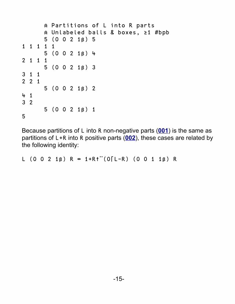
⍝ Partitions of L into R parts ⍝ Unlabeled balls & boxes, ≥1 #bpb 5 (0 0 2 1β) 51 1 1 1 1 5 (0 0 2 1β) 42 1 1 1 5 (0 0 2 1β) 33 1 12 2 1 5 (0 0 2 1β) 24 13 2 5 (0 0 2 1β) 15

Because partitions of L into R non-negative parts (001) is the same as partitions of L+R into R positive parts (002), these cases are related by the following identity:

L (0 0 2 1β) R ↔ 1+R↑¨(0⌈L-R) (0 0 1 1β) R

-15-

Case 010: (Back to FS T able)

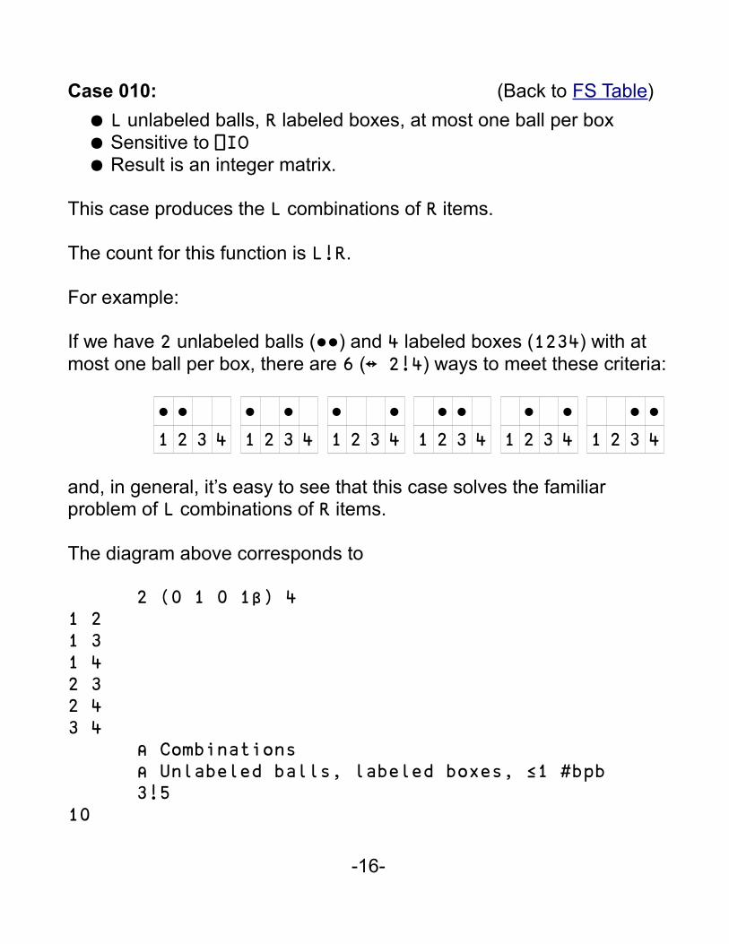
● L unlabeled balls, R labeled boxes, at most one ball per box● Sensitive to ⎕IO● Result is an integer matrix.

This case produces the L combinations of R items.

The count for this function is L!R.

For example:

If we have 2 unlabeled balls (●●) and 4 labeled boxes (1234) with at most one ball per box, there are 6 (↔ 2!4) ways to meet these criteria:

● ●1 2 3 4

● ●1 2 3 4

● ●1 2 3 4

● ●1 2 3 4

● ●1 2 3 4

● ●1 2 3 4

and, in general, it’s easy to see that this case solves the familiar problem of L combinations of R items.

The diagram above corresponds to

2 (0 1 0 1β) 41 21 31 42 32 43 4 ⍝ Combinations ⍝ Unlabeled balls, labeled boxes, ≤1 #bpb 3!510

-16-

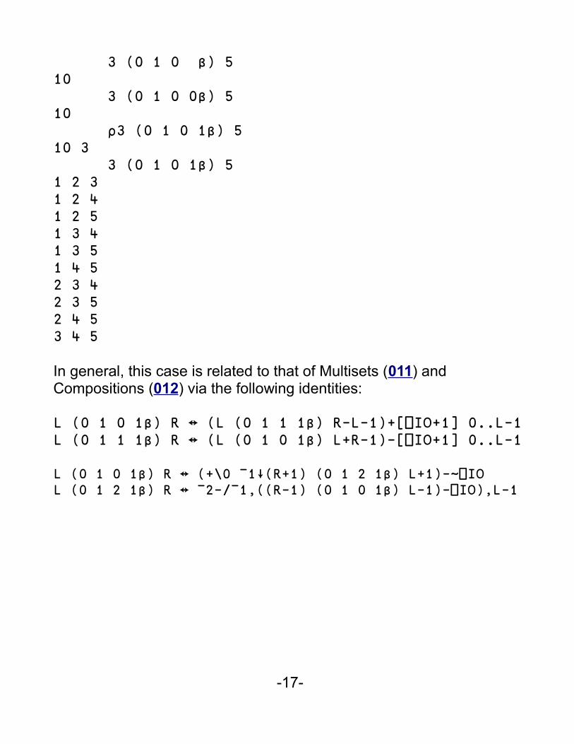
3 (0 1 0 β) 510 3 (0 1 0 0β) 510 ⍴3 (0 1 0 1β) 510 3 3 (0 1 0 1β) 51 2 31 2 41 2 51 3 41 3 51 4 52 3 42 3 52 4 53 4 5

In general, this case is related to that of Multisets (011) and Compositions (012) via the following identities:

L (0 1 0 1β) R ↔ (L (0 1 1 1β) R-L-1)+[⎕IO+1] 0..L-1L (0 1 1 1β) R ↔ (L (0 1 0 1β) L+R-1)-[⎕IO+1] 0..L-1

L (0 1 0 1β) R ↔ (+\0 ¯1↓(R+1) (0 1 2 1β) L+1)-~⎕IOL (0 1 2 1β) R ↔ ¯2-/¯1,((R-1) (0 1 0 1β) L-1)-⎕IO),L-1

-17-

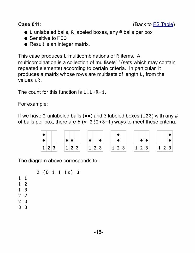
Case 011: (Back to FS T able)

● L unlabeled balls, R labeled boxes, any # balls per box● Sensitive to ⎕IO● Result is an integer matrix.

This case produces L multicombinations of R items. A multicombination is a collection of multisets10 (sets which may contain repeated elements) according to certain criteria. In particular, it produces a matrix whose rows are multisets of length L, from the values ⍳R.

The count for this function is L!L+R-1.

For example:

If we have 2 unlabeled balls (●●) and 3 labeled boxes (123) with any #of balls per box, there are 6 (↔ 2!2+3-1) ways to meet these criteria:

●●1 2 3

● ●1 2 3

● ●1 2 3

●●

1 2 3

● ●1 2 3

●●

1 2 3

The diagram above corresponds to:

2 (0 1 1 1β) 31 11 21 32 22 33 3

-18-

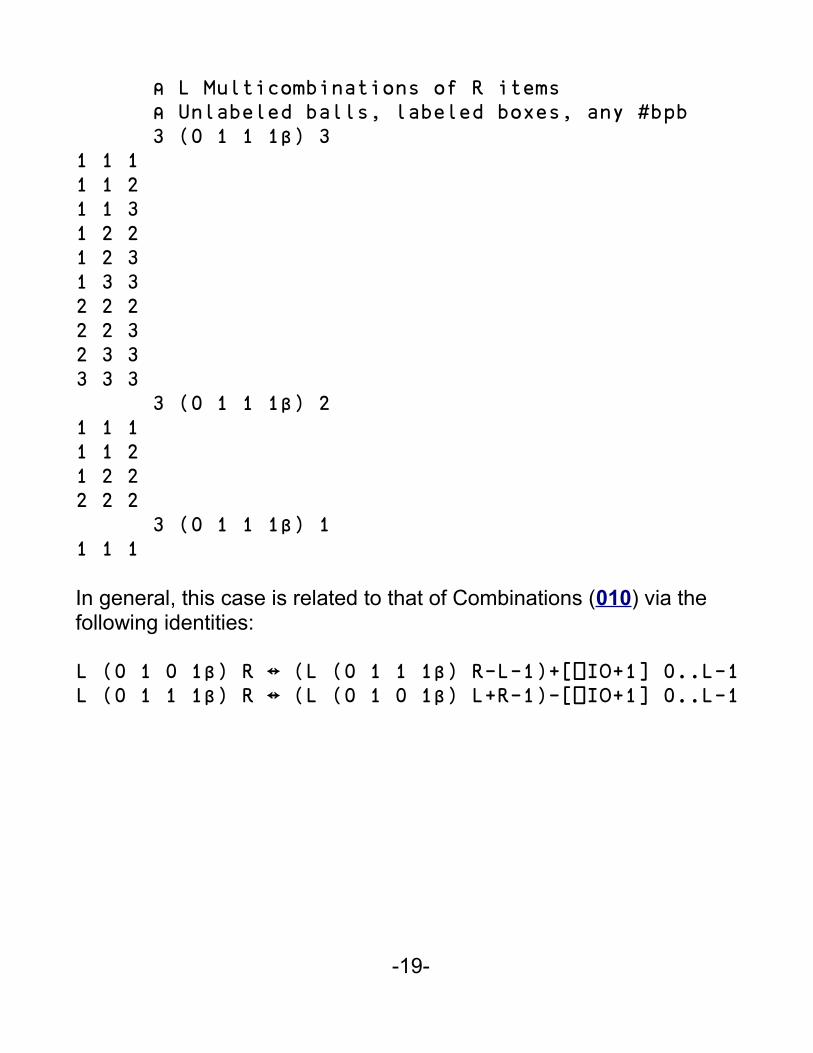
⍝ L Multicombinations of R items ⍝ Unlabeled balls, labeled boxes, any #bpb 3 (0 1 1 1β) 31 1 11 1 21 1 31 2 21 2 31 3 32 2 22 2 32 3 33 3 3 3 (0 1 1 1β) 21 1 11 1 21 2 22 2 2 3 (0 1 1 1β) 11 1 1

In general, this case is related to that of Combinations (010) via the following identities:

L (0 1 0 1β) R ↔ (L (0 1 1 1β) R-L-1)+[⎕IO+1] 0..L-1L (0 1 1 1β) R ↔ (L (0 1 0 1β) L+R-1)-[⎕IO+1] 0..L-1

-19-

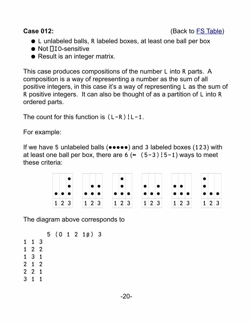
Case 012: (Back to FS T able)

● L unlabeled balls, R labeled boxes, at least one ball per box● Not ⎕IO-sensitive● Result is an integer matrix.

This case produces compositions of the number L into R parts. A composition is a way of representing a number as the sum of all positive integers, in this case it’s a way of representing L as the sum ofR positive integers. It can also be thought of as a partition of L into R ordered parts.

The count for this function is (L-R)!L-1.

For example:

If we have 5 unlabeled balls (●●●●●) and 3 labeled boxes (123) with at least one ball per box, there are 6 (↔ (5-3)!5-1) ways to meet these criteria:

● ●

●●●

1 2 3

●●●●●

1 2 3

●

●●● ●

1 2 3

●● ●

●●

1 2 3

●●●● ●

1 2 3

●●● ● ●1 2 3

The diagram above corresponds to

5 (0 1 2 1β) 31 1 31 2 21 3 12 1 22 2 13 1 1

-20-

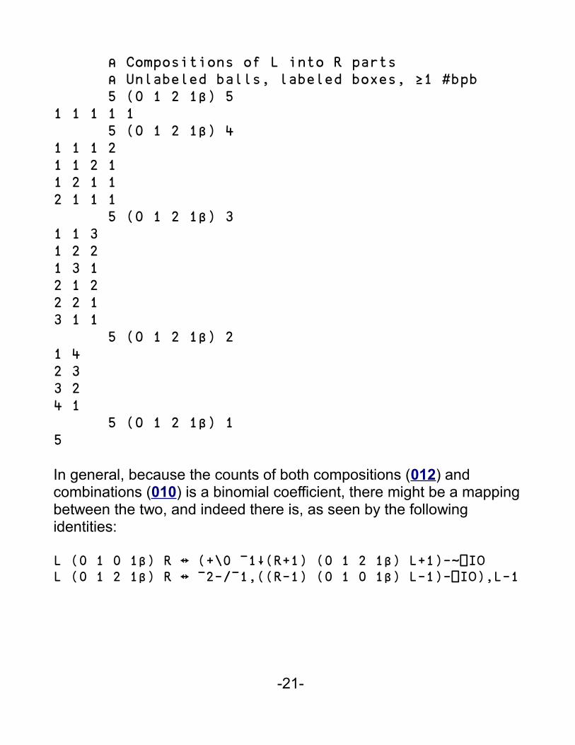
⍝ Compositions of L into R parts ⍝ Unlabeled balls, labeled boxes, ≥1 #bpb 5 (0 1 2 1β) 51 1 1 1 1 5 (0 1 2 1β) 41 1 1 21 1 2 11 2 1 12 1 1 1 5 (0 1 2 1β) 31 1 31 2 21 3 12 1 22 2 13 1 1 5 (0 1 2 1β) 21 42 33 24 1 5 (0 1 2 1β) 15

In general, because the counts of both compositions (012) and combinations (010) is a binomial coefficient, there might be a mapping between the two, and indeed there is, as seen by the following identities:

L (0 1 0 1β) R ↔ (+\0 ¯1↓(R+1) (0 1 2 1β) L+1)-~⎕IOL (0 1 2 1β) R ↔ ¯2-/¯1,((R-1) (0 1 0 1β) L-1)-⎕IO),L-1

-21-

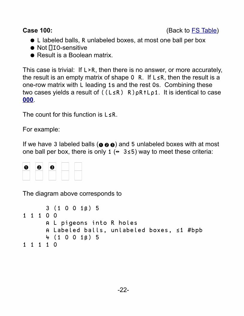
Case 100: (Back to FS T able)

● L labeled balls, R unlabeled boxes, at most one ball per box● Not ⎕IO-sensitive● Result is a Boolean matrix.

This case is trivial: If L>R, then there is no answer, or more accurately,the result is an empty matrix of shape 0 R. If L≤R, then the result is a one-row matrix with L leading 1s and the rest 0s. Combining these two cases yields a result of ((L≤R) R)⍴R↑L⍴1. It is identical to case 000.

The count for this function is L≤R.

For example:

If we have 3 labeled balls ( ❶❷❸) and 5 unlabeled boxes with at most one ball per box, there is only 1 (↔ 3≤5) way to meet these criteria:

❶ ❷ ❸

The diagram above corresponds to

3 (1 0 0 1β) 51 1 1 0 0 ⍝ L pigeons into R holes ⍝ Labeled balls, unlabeled boxes, ≤1 #bpb 4 (1 0 0 1β) 51 1 1 1 0

-22-

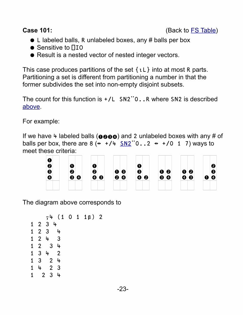
Case 101: (Back to FS T able)

● L labeled balls, R unlabeled boxes, any # balls per box● Sensitive to ⎕IO● Result is a nested vector of nested integer vectors.

This case produces partitions of the set {⍳L} into at most R parts. Partitioning a set is different from partitioning a number in that the former subdivides the set into non-empty disjoint subsets.

The count for this function is +/L SN2¨0..R where SN2 is described above.

For example:

If we have 4 labeled balls (❶❷❸❹) and 2 unlabeled boxes with any # ofballs per box, there are 8 (↔ +/4 SN2¨0..2 ↔ +/0 1 7) ways to meet these criteria:

❶❷❸❹

❶❷❸ ❹

❶❷❹ ❸

❶❷

❸❹

❶❸❹ ❷

❶❸

❷❹

❶❹

❷❸ ❶

❷❸❹

The diagram above corresponds to

⍪4 (1 0 1 1β) 2 1 2 3 4 1 2 3 4 1 2 4 3 1 2 3 4 1 3 4 2 1 3 2 4 1 4 2 3 1 2 3 4

-23-

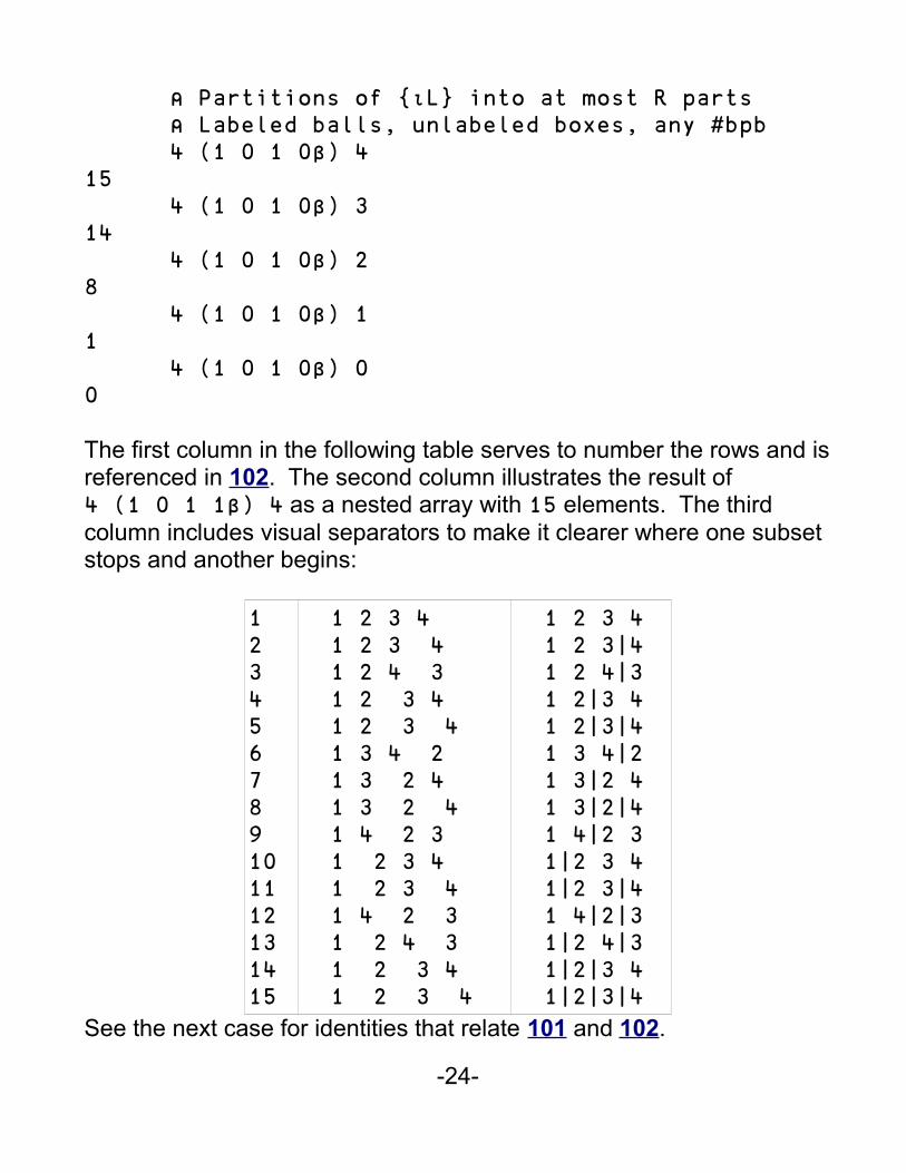
⍝ Partitions of {⍳L} into at most R parts ⍝ Labeled balls, unlabeled boxes, any #bpb 4 (1 0 1 0β) 415 4 (1 0 1 0β) 314 4 (1 0 1 0β) 28 4 (1 0 1 0β) 11 4 (1 0 1 0β) 00

The first column in the following table serves to number the rows and isreferenced in 102. The second column illustrates the result of 4 (1 0 1 1β) 4 as a nested array with 15 elements. The third column includes visual separators to make it clearer where one subset stops and another begins:

123456789101112131415

1 2 3 4 1 2 3 4 1 2 4 3 1 2 3 4 1 2 3 4 1 3 4 2 1 3 2 4 1 3 2 4 1 4 2 3 1 2 3 4 1 2 3 4 1 4 2 3 1 2 4 3 1 2 3 4 1 2 3 4

1 2 3 4 1 2 3|4 1 2 4|3 1 2|3 4 1 2|3|4 1 3 4|2 1 3|2 4 1 3|2|4 1 4|2 3 1|2 3 4 1|2 3|4 1 4|2|3 1|2 4|3 1|2|3 4 1|2|3|4

See the next case for identities that relate 101 and 102.

-24-

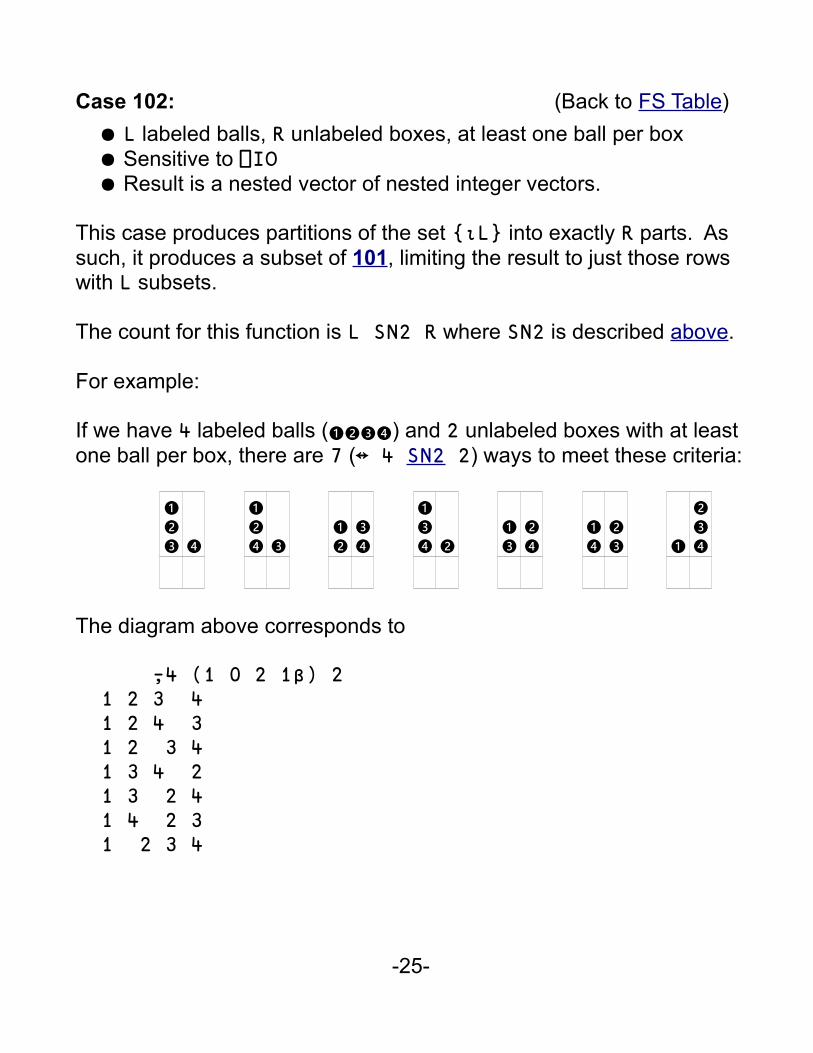
Case 102: (Back to FS T able)

● L labeled balls, R unlabeled boxes, at least one ball per box● Sensitive to ⎕IO● Result is a nested vector of nested integer vectors.

This case produces partitions of the set {⍳L} into exactly R parts. As such, it produces a subset of 101, limiting the result to just those rows with L subsets.

The count for this function is L SN2 R where SN2 is described above.

For example:

If we have 4 labeled balls (❶❷❸❹) and 2 unlabeled boxes with at least one ball per box, there are 7 (↔ 4 SN2 2) ways to meet these criteria:

❶❷❸ ❹

❶❷❹ ❸

❶❷

❸❹

❶❸❹ ❷

❶❸

❷❹

❶❹

❷❸ ❶

❷❸❹

The diagram above corresponds to

⍪4 (1 0 2 1β) 2 1 2 3 4 1 2 4 3 1 2 3 4 1 3 4 2 1 3 2 4 1 4 2 3 1 2 3 4

-25-

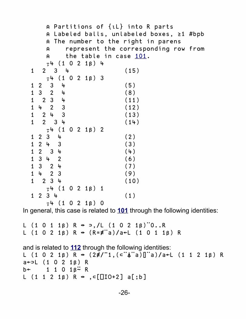
⍝ Partitions of {⍳L} into R parts ⍝ Labeled balls, unlabeled boxes, ≥1 #bpb ⍝ The number to the right in parens ⍝ represent the corresponding row from ⍝ the table in case 101. ⍪4 (1 0 2 1β) 4 1 2 3 4 (15) ⍪4 (1 0 2 1β) 3 1 2 3 4 (5) 1 3 2 4 (8) 1 2 3 4 (11) 1 4 2 3 (12) 1 2 4 3 (13) 1 2 3 4 (14) ⍪4 (1 0 2 1β) 2 1 2 3 4 (2) 1 2 4 3 (3) 1 2 3 4 (4) 1 3 4 2 (6) 1 3 2 4 (7) 1 4 2 3 (9) 1 2 3 4 (10) ⍪4 (1 0 2 1β) 1 1 2 3 4 (1) ⍪4 (1 0 2 1β) 0In general, this case is related to 101 through the following identities:

L (1 0 1 1β) R ↔ ⊃,/L (1 0 2 1β)¨0..RL (1 0 2 1β) R ↔ (R=≢¨a)/a←L (1 0 1 1β) R

and is related to 112 through the following identities:L (1 0 2 1β) R ↔ (2≢/¯1,(⊂¨⍋¨a)⌷¨a)/a←L (1 1 2 1β) Ra←⊃L (1 0 2 1β) Rb← 1 1 0 1β⍨ RL (1 1 2 1β) R ↔ ,⊂[⎕IO+2] a[;b]

-26-

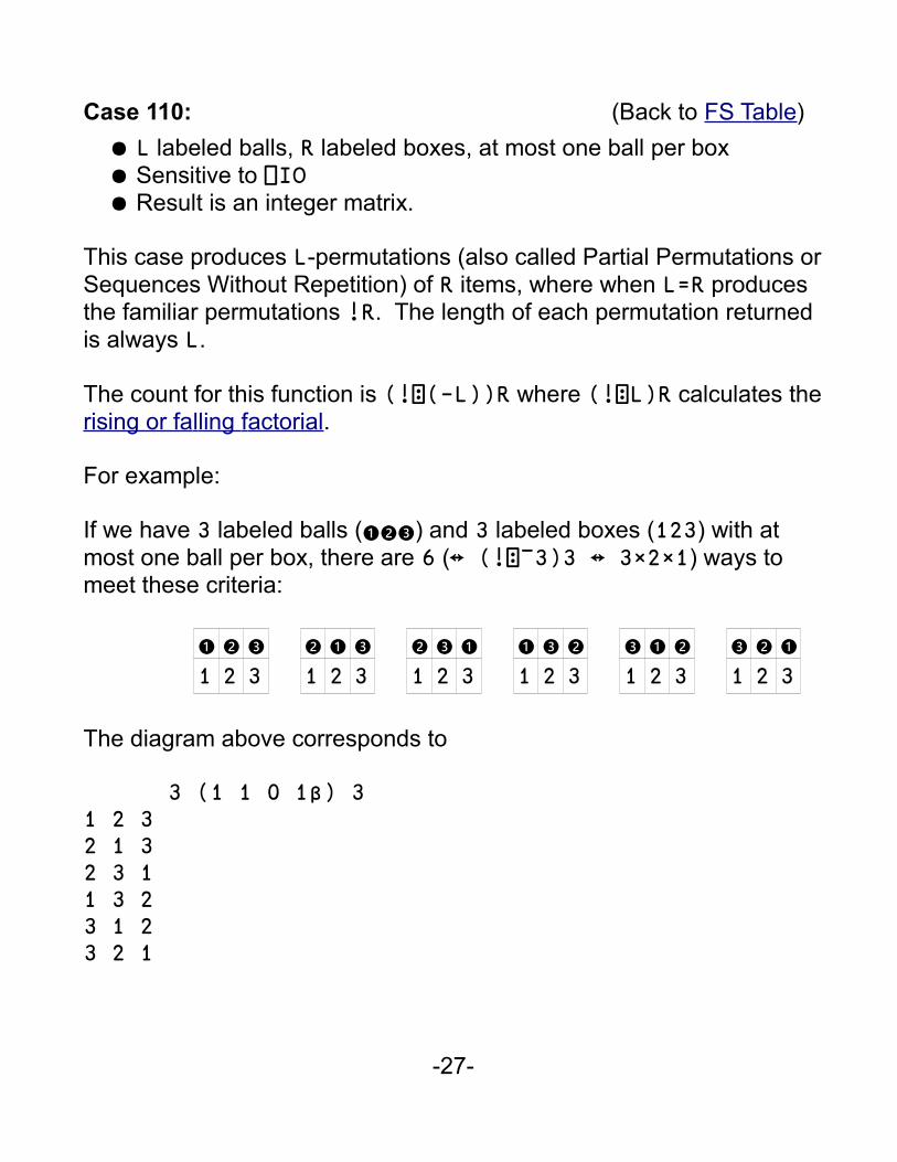
Case 110: (Back to FS T able)

● L labeled balls, R labeled boxes, at most one ball per box● Sensitive to ⎕IO● Result is an integer matrix.

This case produces L-permutations (also called Partial Permutations orSequences Without Repetition) of R items, where when L=R produces the familiar permutations !R. The length of each permutation returned is always L.

The count for this function is (!⍠(-L))R where (!⍠L)R calculates therising or fa l ling f actorial.

For example:

If we have 3 labeled balls (❶❷❸) and 3 labeled boxes (123) with at most one ball per box, there are 6 (↔ (!⍠¯3)3 ↔ 3×2×1) ways to meet these criteria:

❶ ❷ ❸

1 2 3❷ ❶ ❸

1 2 3❷ ❸ ❶

1 2 3❶ ❸ ❷

1 2 3❸ ❶ ❷

1 2 3❸ ❷ ❶

1 2 3

The diagram above corresponds to

3 (1 1 0 1β) 31 2 32 1 32 3 11 3 23 1 23 2 1

-27-

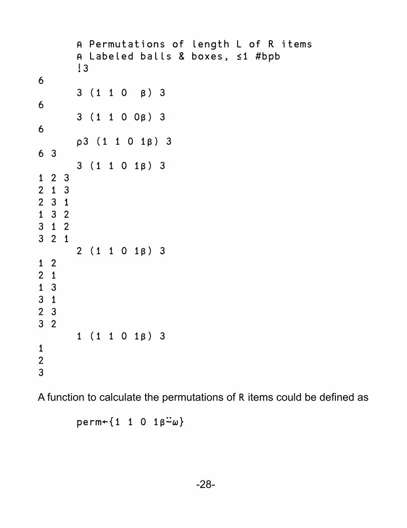
⍝ Permutations of length L of R items ⍝ Labeled balls & boxes, ≤1 #bpb !36 3 (1 1 0 β) 36 3 (1 1 0 0β) 36 ⍴3 (1 1 0 1β) 36 3 3 (1 1 0 1β) 31 2 32 1 32 3 11 3 23 1 23 2 1 2 (1 1 0 1β) 31 22 11 33 12 33 2 1 (1 1 0 1β) 3123

A function to calculate the permutations of R items could be defined as

perm←{1 1 0 1β⍨⍵}

-28-

Case 111: (Back to FS T able)

● L labeled balls, R labeled boxes, any # balls per box● Sensitive to ⎕IO● Result is an integer matrix.

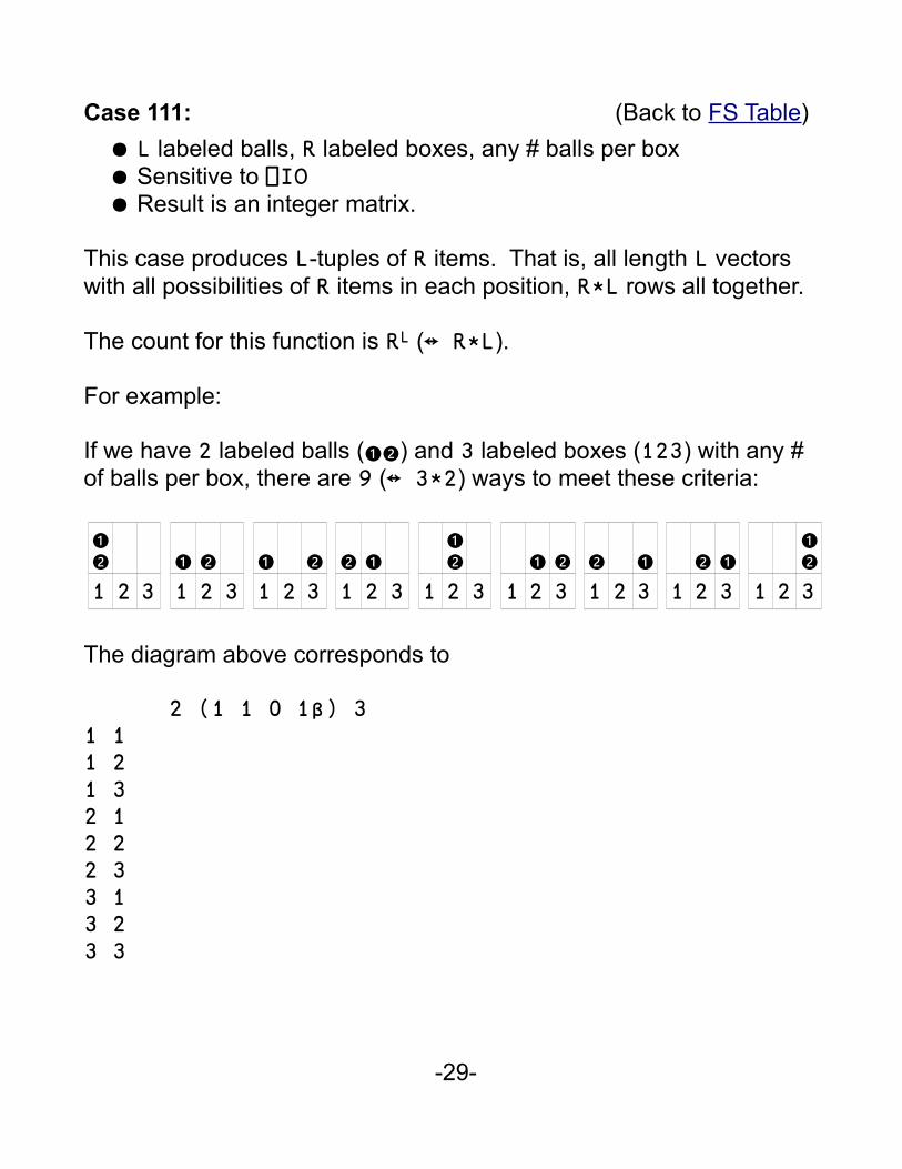
This case produces L-tuples of R items. That is, all length L vectors with all possibilities of R items in each position, R*L rows all together.

The count for this function is RL (↔ R*L).

For example:

If we have 2 labeled balls (❶❷) and 3 labeled boxes (123) with any # of balls per box, there are 9 (↔ 3*2) ways to meet these criteria:

❶❷

1 2 3❶ ❷

1 2 3❶ ❷

1 2 3❷ ❶

1 2 3

❶❷

1 2 3❶ ❷

1 2 3❷ ❶

1 2 3❷ ❶

1 2 3

❶❷

1 2 3

The diagram above corresponds to

2 (1 1 0 1β) 31 11 21 32 12 22 33 13 23 3

-29-

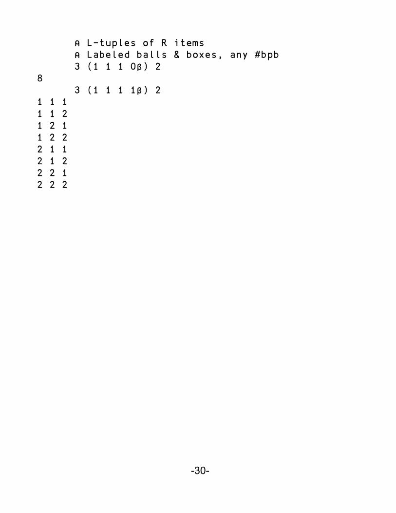
⍝ L-tuples of R items ⍝ Labeled balls & boxes, any #bpb 3 (1 1 1 0β) 28 3 (1 1 1 1β) 21 1 11 1 21 2 11 2 22 1 12 1 22 2 12 2 2

-30-

Case 112: (Back to FS T able)

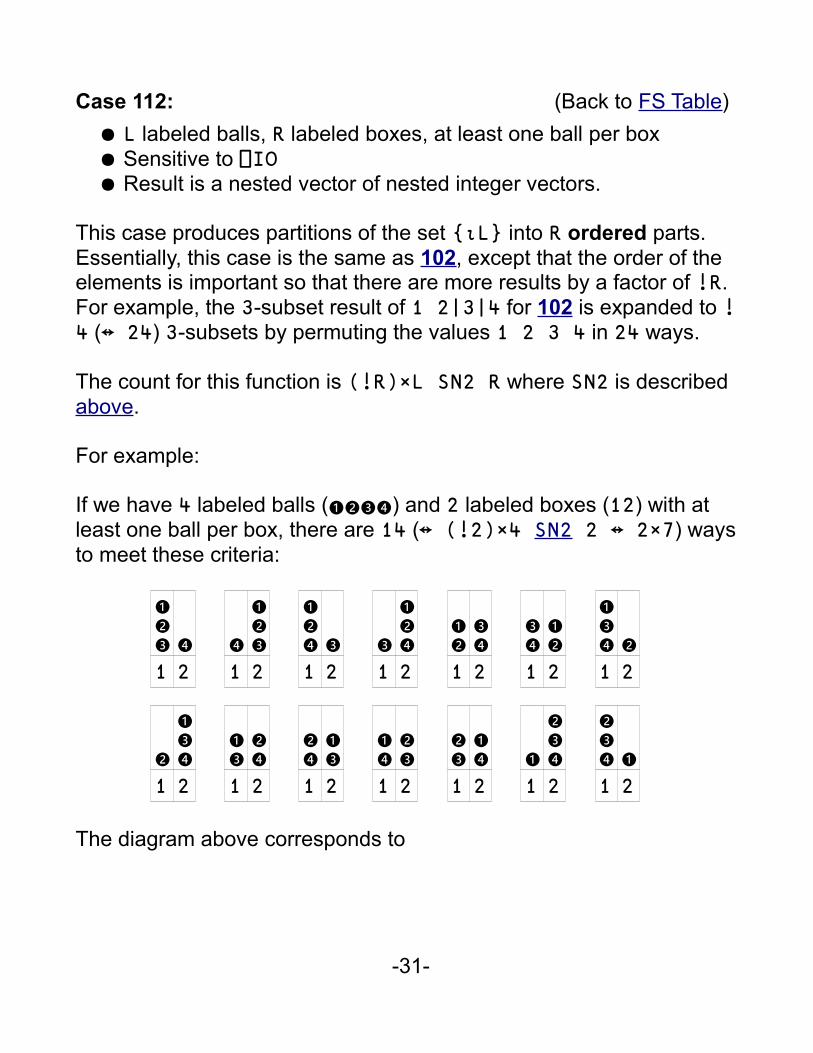
● L labeled balls, R labeled boxes, at least one ball per box● Sensitive to ⎕IO● Result is a nested vector of nested integer vectors.

This case produces partitions of the set {⍳L} into R ordered parts. Essentially, this case is the same as 102, except that the order of the elements is important so that there are more results by a factor of !R. For example, the 3-subset result of 1 2|3|4 for 102 is expanded to !4 (↔ 24) 3-subsets by permuting the values 1 2 3 4 in 24 ways.

The count for this function is (!R)×L SN2 R where SN2 is described above.

For example:

If we have 4 labeled balls (❶❷❸❹) and 2 labeled boxes (12) with at least one ball per box, there are 14 (↔ (!2)×4 SN2 2 ↔ 2×7) ways to meet these criteria:

❶❷❸ ❹

1 2❹

❶❷❸

1 2

❶❷❹ ❸

1 2❸

❶❷❹

1 2

❶❷

❸❹

1 2

❸❹

❶❷

1 2

❶❸❹ ❷

1 2

❷

❶❸❹

1 2

❶❸

❷❹

1 2

❷❹

❶❸

1 2

❶❹

❷❸

1 2

❷❸

❶❹

1 2❶

❷❸❹

1 2

❷❸❹ ❶

1 2

The diagram above corresponds to

-31-

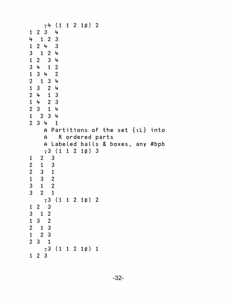
⍪4 (1 1 2 1β) 2 1 2 3 4 4 1 2 3 1 2 4 3 3 1 2 4 1 2 3 4 3 4 1 2 1 3 4 2 2 1 3 4 1 3 2 4 2 4 1 3 1 4 2 3 2 3 1 4 1 2 3 4 2 3 4 1 ⍝ Partitions of the set {⍳L} into ⍝ R ordered parts ⍝ Labeled balls & boxes, any #bpb ⍪3 (1 1 2 1β) 3 1 2 3 2 1 3 2 3 1 1 3 2 3 1 2 3 2 1 ⍪3 (1 1 2 1β) 2 1 2 3 3 1 2 1 3 2 2 1 3 1 2 3 2 3 1 ⍪3 (1 1 2 1β) 1 1 2 3

-32-

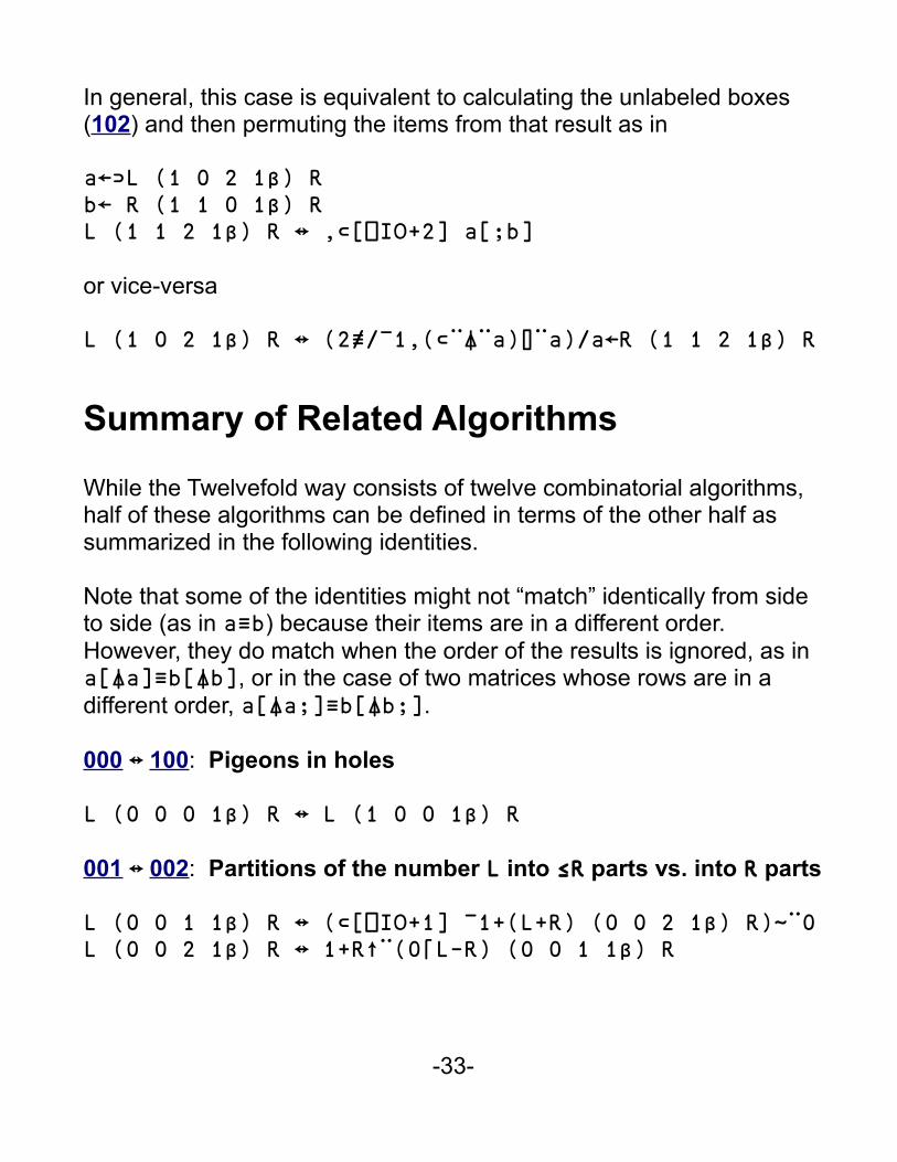
In general, this case is equivalent to calculating the unlabeled boxes (102) and then permuting the items from that result as in

a←⊃L (1 0 2 1β) Rb← R (1 1 0 1β) RL (1 1 2 1β) R ↔ ,⊂[⎕IO+2] a[;b]

or vice-versa

L (1 0 2 1β) R ↔ (2≢/¯1,(⊂¨⍋¨a)⌷¨a)/a←R (1 1 2 1β) R

Summary of Related Algorithms

While the Twelvefold way consists of twelve combinatorial algorithms, half of these algorithms can be defined in terms of the other half as summarized in the following identities.

Note that some of the identities might not “match” identically from side to side (as in a≡b) because their items are in a different order. However, they do match when the order of the results is ignored, as in a[⍋a]≡b[⍋b], or in the case of two matrices whose rows are in a different order, a[⍋a;]≡b[⍋b;].

000 ↔ 100: Pigeons in holes

L (0 0 0 1β) R ↔ L (1 0 0 1β) R

001 ↔ 002: Partitions of the number L into ≤R parts vs. into R parts

L (0 0 1 1β) R ↔ (⊂[⎕IO+1] ¯1+(L+R) (0 0 2 1β) R)~¨0L (0 0 2 1β) R ↔ 1+R↑¨(0⌈L-R) (0 0 1 1β) R

-33-

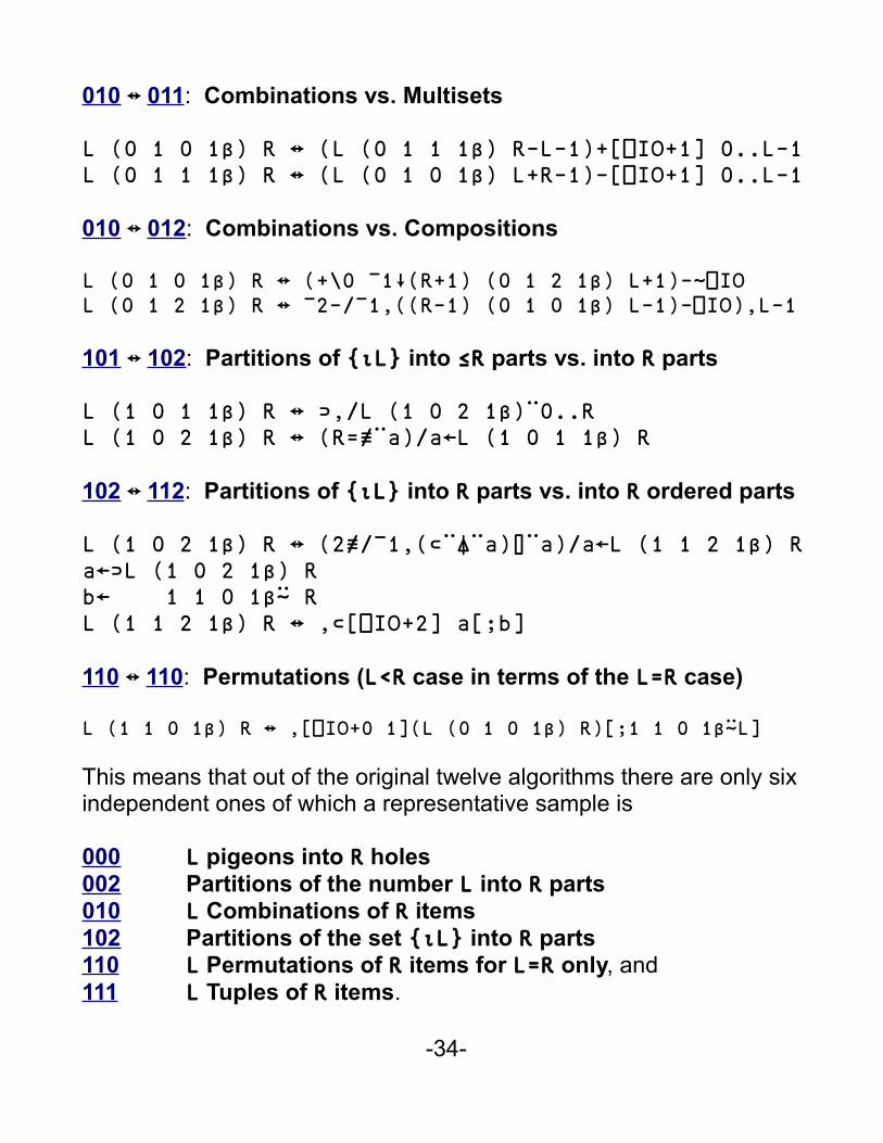
010 ↔ 011: Combinations vs. Multisets

L (0 1 0 1β) R ↔ (L (0 1 1 1β) R-L-1)+[⎕IO+1] 0..L-1L (0 1 1 1β) R ↔ (L (0 1 0 1β) L+R-1)-[⎕IO+1] 0..L-1

010 ↔ 012: Combinations vs. Compositions

L (0 1 0 1β) R ↔ (+\0 ¯1↓(R+1) (0 1 2 1β) L+1)-~⎕IOL (0 1 2 1β) R ↔ ¯2-/¯1,((R-1) (0 1 0 1β) L-1)-⎕IO),L-1

101 ↔ 102: Partitions of {⍳L} into ≤R parts vs. into R parts

L (1 0 1 1β) R ↔ ⊃,/L (1 0 2 1β)¨0..RL (1 0 2 1β) R ↔ (R=≢¨a)/a←L (1 0 1 1β) R

102 ↔ 112: Partitions of {⍳L} into R parts vs. into R ordered parts

L (1 0 2 1β) R ↔ (2≢/¯1,(⊂¨⍋¨a)⌷¨a)/a←L (1 1 2 1β) Ra←⊃L (1 0 2 1β) Rb← 1 1 0 1β⍨ RL (1 1 2 1β) R ↔ ,⊂[⎕IO+2] a[;b]

110 ↔ 110: Permutations (L<R case in terms of the L=R case)

L (1 1 0 1β) R ↔ ,[⎕IO+0 1](L (0 1 0 1β) R)[;1 1 0 1β⍨L]

This means that out of the original twelve algorithms there are only six independent ones of which a representative sample is

000 L pigeons into R holes002 Partitions of the number L into R parts010 L Combinations of R items102 Partitions of the set {⍳L} into R parts110 L Permutations of R items for L=R only, and111 L Tuples of R items.

-34-

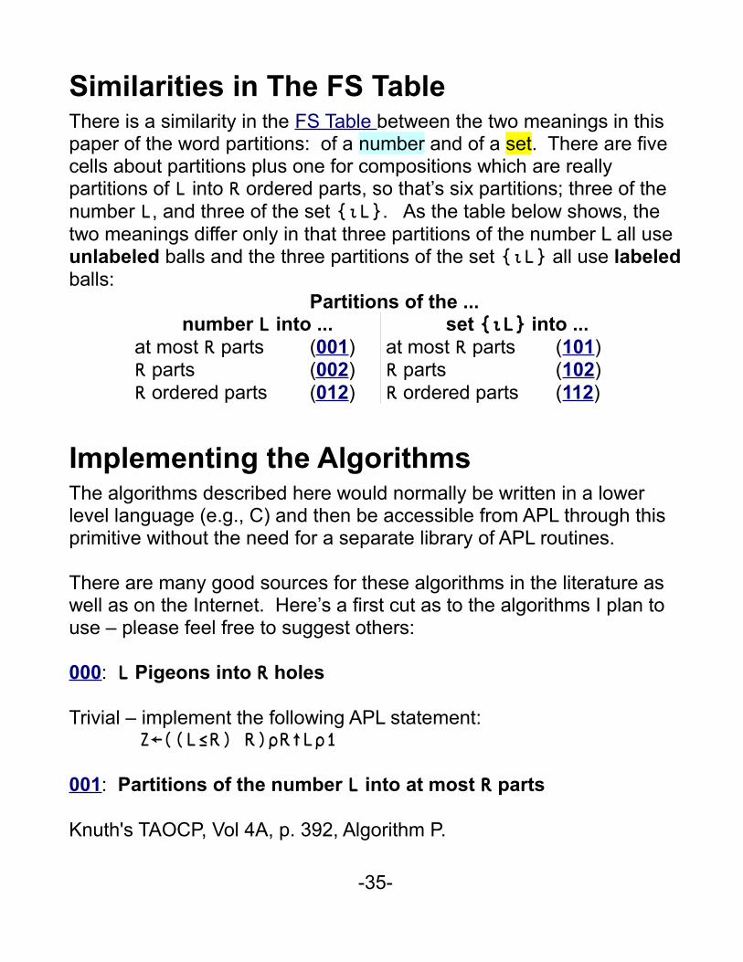
Similarities in The FS TableThere is a similarity in the FS Table between the two meanings in this paper of the word partitions: of a number and of a set. There are five cells about partitions plus one for compositions which are really partitions of L into R ordered parts, so that’s six partitions; three of the number L, and three of the set {⍳L}. As the table below shows, the two meanings differ only in that three partitions of the number L all use unlabeled balls and the three partitions of the set {⍳L} all use labeledballs:

Partitions of the ...number L into ... set {⍳L} into ...

at most R parts (001) at most R parts (101)R parts (002) R parts (102)R ordered parts (012) R ordered parts (112)

Implementing the AlgorithmsThe algorithms described here would normally be written in a lower level language (e.g., C) and then be accessible from APL through this primitive without the need for a separate library of APL routines.

There are many good sources for these algorithms in the literature as well as on the Internet. Here’s a first cut as to the algorithms I plan to use – please feel free to suggest others:

000: L Pigeons into R holes

Trivial – implement the following APL statement: Z←((L≤R) R)⍴R↑L⍴1

001: Partitions of the number L into at most R parts

Knuth's TAOCP, Vol 4A, p. 392, Algorithm P.

-35-

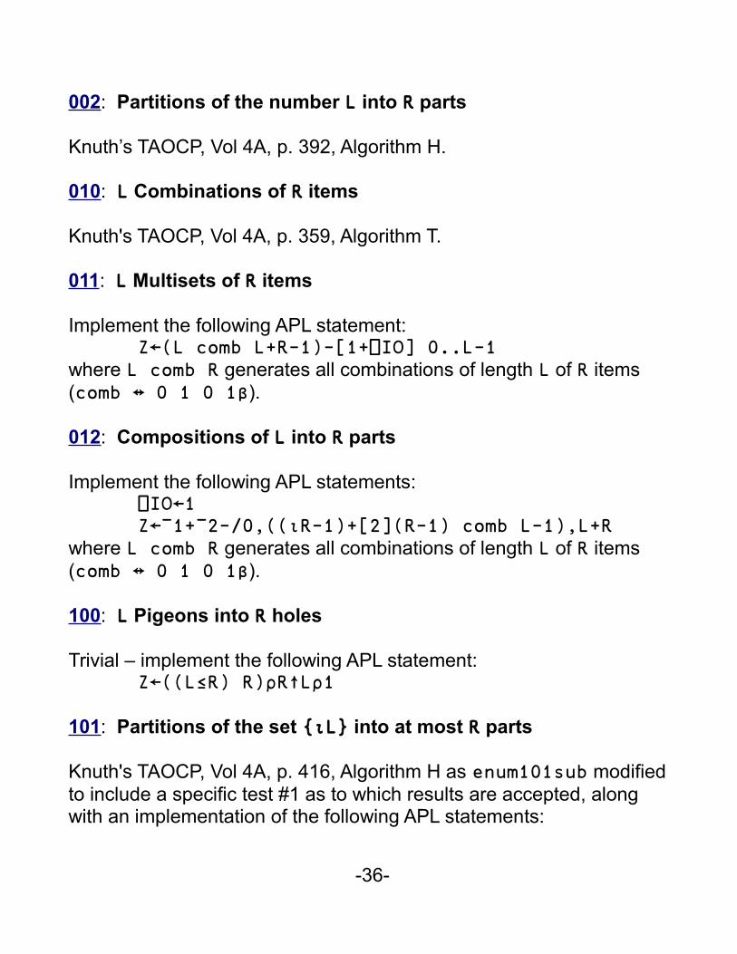
002: Partitions of the number L into R parts

Knuth’s TAOCP, Vol 4A, p. 392, Algorithm H.

010: L Combinations of R items

Knuth's TAOCP, Vol 4A, p. 359, Algorithm T.

011: L Multisets of R items

Implement the following APL statement: Z←(L comb L+R-1)-[1+⎕IO] 0..L-1where L comb R generates all combinations of length L of R items (comb ↔ 0 1 0 1β).

012: Compositions of L into R parts

Implement the following APL statements: ⎕IO←1 Z←¯1+¯2-/0,((⍳R-1)+[2](R-1) comb L-1),L+Rwhere L comb R generates all combinations of length L of R items (comb ↔ 0 1 0 1β).

100: L Pigeons into R holes

Trivial – implement the following APL statement: Z←((L≤R) R)⍴R↑L⍴1

101: Partitions of the set {⍳L} into at most R parts

Knuth's TAOCP, Vol 4A, p. 416, Algorithm H as enum101sub modified to include a specific test #1 as to which results are accepted, along with an implementation of the following APL statements:

-36-

b←⊂[1+⎕IO] L enum101sub R Z←(1+(⊂¨⍋¨b)⌷¨b)⊂¨⍋¨b

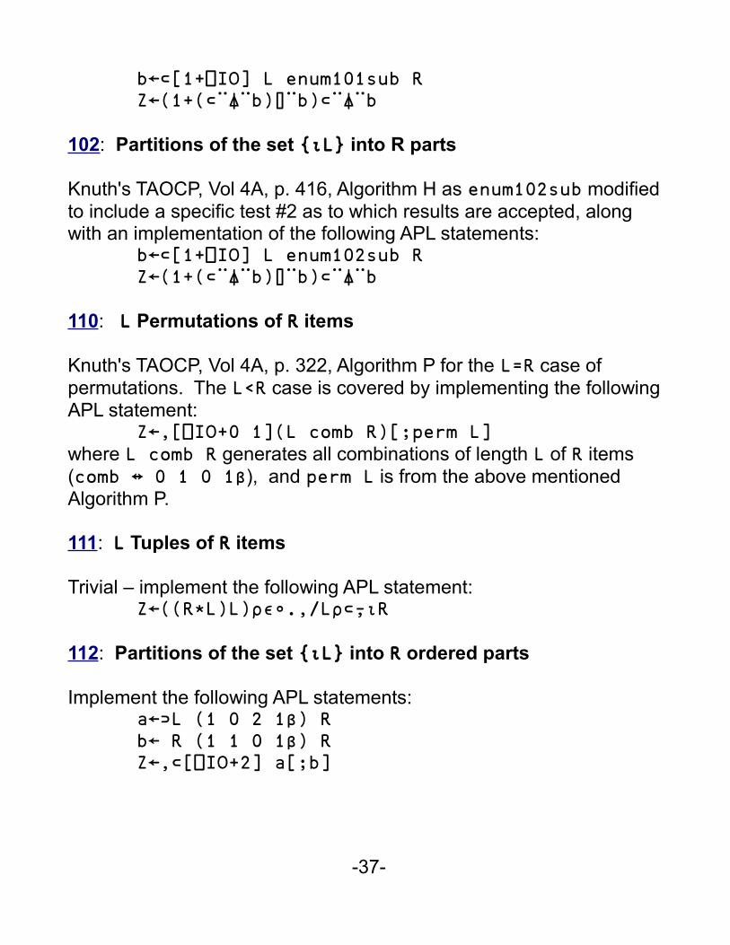
102: Partitions of the set {⍳L} into R parts

Knuth's TAOCP, Vol 4A, p. 416, Algorithm H as enum102sub modified to include a specific test #2 as to which results are accepted, along with an implementation of the following APL statements: b←⊂[1+⎕IO] L enum102sub R Z←(1+(⊂¨⍋¨b)⌷¨b)⊂¨⍋¨b

110: L Permutations of R items

Knuth's TAOCP, Vol 4A, p. 322, Algorithm P for the L=R case of permutations. The L<R case is covered by implementing the following APL statement: Z←,[⎕IO+0 1](L comb R)[;perm L]where L comb R generates all combinations of length L of R items (comb ↔ 0 1 0 1β), and perm L is from the above mentioned Algorithm P.

111: L Tuples of R items

Trivial – implement the following APL statement: Z←((R*L)L)⍴∊∘.,/L⍴⊂⍪⍳R

112: Partitions of the set {⍳L} into R ordered parts

Implement the following APL statements: a←⊃L (1 0 2 1β) R b← R (1 1 0 1β) R Z←,⊂[⎕IO+2] a[;b]

-37-

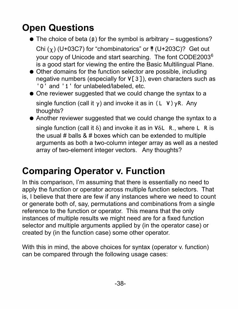
Open Questions● The choice of beta (β) for the symbol is arbitrary – suggestions?

Chi (χ) (U+03C7) for “chombinatorics” or ‼ (U+203C)? Get out your copy of Unicode and start searching. The font CODE20036 is a good start for viewing the entire the Basic Multilingual Plane.

● Other domains for the function selector are possible, including negative numbers (especially for V[3]), even characters such as '0' and '1' for unlabeled/labeled, etc.

● One reviewer suggested that we could change the syntax to a

single function (call it γ) and invoke it as in (L V)γR. Any thoughts?

● Another reviewer suggested that we could change the syntax to a

single function (call it δ) and invoke it as in VδL R., where L R is the usual # balls & # boxes which can be extended to multiple arguments as both a two-column integer array as well as a nestedarray of two-element integer vectors. Any thoughts?

Comparing Operator v. FunctionIn this comparison, I’m assuming that there is essentially no need to apply the function or operator across multiple function selectors. That is, I believe that there are few if any instances where we need to count or generate both of, say, permutations and combinations from a single reference to the function or operator. This means that the only instances of multiple results we might need are for a fixed function selector and multiple arguments applied by (in the operator case) or created by (in the function case) some other operator.

With this in mind, the above choices for syntax (operator v. function) can be compared through the following usage cases:

-38-

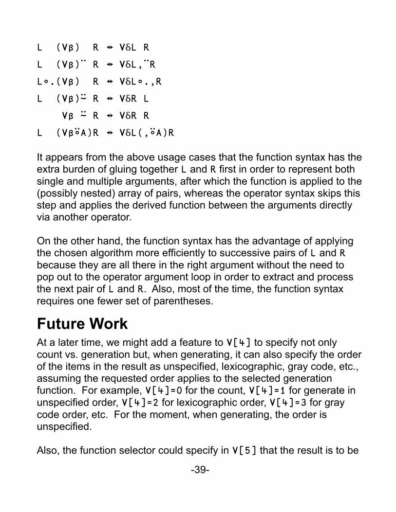
L (Vβ) R ↔ VδL R

L (Vβ)¨ R ↔ VδL,¨R

L∘.(Vβ) R ↔ VδL∘.,R

L (Vβ)⍨ R ↔ VδR L

Vβ ⍨ R ↔ VδR R

L (Vβ⍤A)R ↔ VδL(,⍤A)R

It appears from the above usage cases that the function syntax has theextra burden of gluing together L and R first in order to represent both single and multiple arguments, after which the function is applied to the(possibly nested) array of pairs, whereas the operator syntax skips thisstep and applies the derived function between the arguments directly via another operator.

On the other hand, the function syntax has the advantage of applying the chosen algorithm more efficiently to successive pairs of L and R because they are all there in the right argument without the need to pop out to the operator argument loop in order to extract and process the next pair of L and R. Also, most of the time, the function syntax requires one fewer set of parentheses.

Future WorkAt a later time, we might add a feature to V[4] to specify not only count vs. generation but, when generating, it can also specify the orderof the items in the result as unspecified, lexicographic, gray code, etc., assuming the requested order applies to the selected generation function. For example, V[4]=0 for the count, V[4]=1 for generate in unspecified order, V[4]=2 for lexicographic order, V[4]=3 for gray code order, etc. For the moment, when generating, the order is unspecified.

Also, the function selector could specify in V[5] that the result is to be

-39-

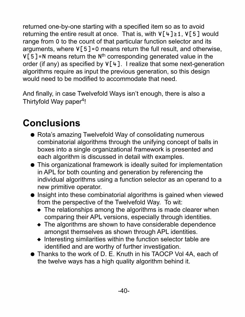
returned one-by-one starting with a specified item so as to avoid returning the entire result at once. That is, with V[4]≥1, V[5] would range from 0 to the count of that particular function selector and its arguments, where V[5]=0 means return the full result, and otherwise, V[5]=N means return the Nth corresponding generated value in the order (if any) as specified by V[4]. I realize that some next-generationalgorithms require as input the previous generation, so this design would need to be modified to accommodate that need.

And finally, in case Twelvefold Ways isn’t enough, there is also a Thirtyfold Way paper4!

Conclusions● Rota’s amazing Twelvefold Way of consolidating numerous

combinatorial algorithms through the unifying concept of balls in boxes into a single organizational framework is presented and each algorithm is discussed in detail with examples.

● This organizational framework is ideally suited for implementation in APL for both counting and generation by referencing the individual algorithms using a function selector as an operand to a new primitive operator.

● Insight into these combinatorial algorithms is gained when viewedfrom the perspective of the Twelvefold Way. To wit: The relationships among the algorithms is made clearer when

comparing their APL versions, especially through identities. The algorithms are shown to have considerable dependence

amongst themselves as shown through APL identities. Interesting similarities within the function selector table are

identified and are worthy of further investigation.● Thanks to the work of D. E. Knuth in his TAOCP Vol 4A, each of

the twelve ways has a high quality algorithm behind it.

-40-

● Finally, APL programmers need no longer search for the fastest APL program to generate any of several combinatorial counts or generations as the fastest way is now available primitively.

Online VersionThis paper is an ongoing effort and can be out-of-date the next day. Tofind the most recent version, go to http://sudleyplace.com/APL / and look for the title of this paper on that page. There is also a workspace online that models this primitive with the user-defined operator beta used in place of the symbol β: http://www.nars2000.org/workspaces/. In your browser, right click on the workspace name and choose “Save Link As...” or “Save target as” to download the workspace to your local hard drive and then )LOAD it from there from within NARS2000.

References1. Stanley, Richard P., "Enumerative Combinatorics", Volume 1, 2nd

edition, Cambridge University Press, p. 71, ISBN 0-521-66351-22. Wikipedia, "Twelvefold Way",

https://en.wikipedia.org/wiki/Twelvefold_way3. Knuth, Donald E., “The Art of Computer Programming”, Addison

Wesley, Volume 4A, Combinatorial Algorithms, p. 390, ISBN 0-201-89685-0

4. Proctor, Robert A., “Let’s Expand Rota’s Twelvefold Way For Counting Partitions”, http://www.math.unc.edu/Faculty/rap/30FoldWay.pdf

5. Wikipedia, “Stirling numbers of the second kind”, https://en.wikipedia.org/wiki/Stirling_numbers_of_the_second_kind

6. CODE2003, http://www.fontspace.com/st-gigafont-typefaces/code2003

-41-

7. Wikipedia, “Partitions: Restricted part size or number of parts”, https://en.wikipedia.org/wiki/Partition_(number_theory)#Restricted_part_size_or_number_of_parts

8. NARS2000 Wiki, “Primes”, http://wiki.nars2000.org/index.php/Primes

9. “Hypercomplex Numbers in APL”, http://www.sudleyplace.com/APL/Hypercomplex%20Numbers%20in%20APL.pdf

10. NARS2000 Wiki, “Multisets”, http://wiki.nars2000.org/index.php/Multisets

11. Wikipedia, “TwelveFold Way”, https://en.wikipedia.org/wiki/Twelvefold_way#case_fnx

-42-