Annual Report 1995 of the CODE Analysis

Center of the IGS

M. Rothacher, G. Beutler, E. Brockmann, L. Mervart,

S. Schaer, T. A. Springer

Astronomical Institute, University of Bern

U. Wild, A. Wiget

Federal Office of Topography, Wabern

C. Boucher

Institut Geographique National, Paris

H. Seeger

Institut fur Angewandte Geodasie, Frankfurt

1. INTRODUCTION AND OVERVIEW

CODE, the Center for Orbit Determination in Europe, is a joint venture of the followinginstitutions:

• the Federal Office of Topography (L+T), Wabern, Switzerland

• the Institut Geographique National (IGN), Paris, France

• the Institute for Applied Geodesy (IfAG), Frankfurt, Germany

• the Astronomical Institute of the University of Berne (AIUB), Berne, Switzerland

The CODE Analysis Center, according to its name and the participating institutions, laysspecial emphasis on Europe in two respects:

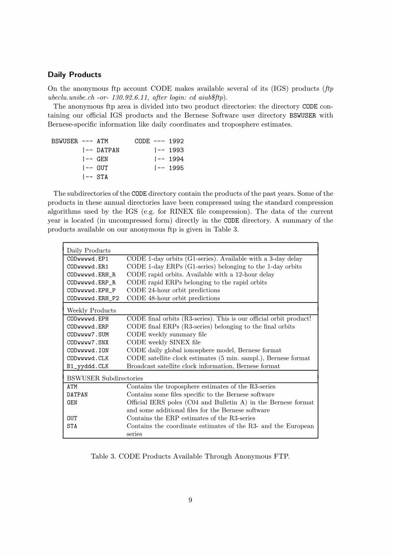
• The European region is clearly over-represented in the global CODE solutions (aboutone third of the 75 sites used in the global solutions are European sites). This shouldguarantee that the CODE orbits are of as good a quality as possible over Europe.

• A special solution for approximately 30 European sites is routinely computed with adelay of about 14 days using the final CODE orbits to monitor the European sitesand reference frame.

1

The CODE is located at the AIUB and uses a cluster of DEC Alpha processors for thedaily IGS processing. The data is analysed with the Bernese GPS Software Version 4.0.This report covers the time period from January 1995 to April 1996. During this period

the number of sites in “our” global network — and therefore also the number of observationsand parameters — was again growing considerably. Table 1 gives an overview of the dailyworkload at CODE since the beginning of the IGS (test campaign) in June 1992.

Solution Characteristic Number Used in Daily CODE ProcessingJune 1992 Jan. 1993 Jan. 1994 Jan. 1995 Jan. 1996

Number of Satellites 19 21 26 25 25Number of Stations 25 28 38 49 72Number of Observations 50’000 60’000 140’000 210’000 250’000Total Number of Param. 2’000 2’300 6’000 9’000 12’000Ambiguity Parameters 1’500 1’800 5’300 8’000 10’500

Table 1. Workload of the Routine 3-Day Solutions at CODE from 1992 to 1996.

Figure 1 shows the number of global sites processed by CODE and the number of para-meters in the ambiguity-free and ambiguity-fixed 3-day solutions during the time intervaldiscussed in this report.

Figure 1. Statistics of Global 3-Day Solutions Computed at CODE

2

Whereas the number of parameters in the ambiguity-free case is increasing in a similar wayas the number of sites, there is no such increase visible in the ambiguity-fixed solutions dueto a shortening of the average baseline length in the global network and due to improvementsin the ambiguity resolution strategy. On day 084, 1996, the ambiguity-free 3-day solutionwas discontinued.Not only the size of the solutions was increasing over time but also the number of different

solutions produced at CODE: in addition to the solutions already computed day-by-day inJanuary 1995, CODE is now running the ambiguity resolution step and the ambiguity-fixed 1- and 3-day solutions, satellite and receiver clock estimation, a special Europeansolution, ionosphere model computations, rapid orbit solutions, and last but not least anorbit prediction procedure was implemented. The daily processing as it is implemented atCODE at present (April 1996) is outlined in Section 2.During the last year many new developments were taking place at the CODE Analysis

Center. They are described in more detail in the following sections. Table 2 summarizesmajor changes during the time period covered by this report.

2. DAILY ROUTINE PROCESSING AT CODE

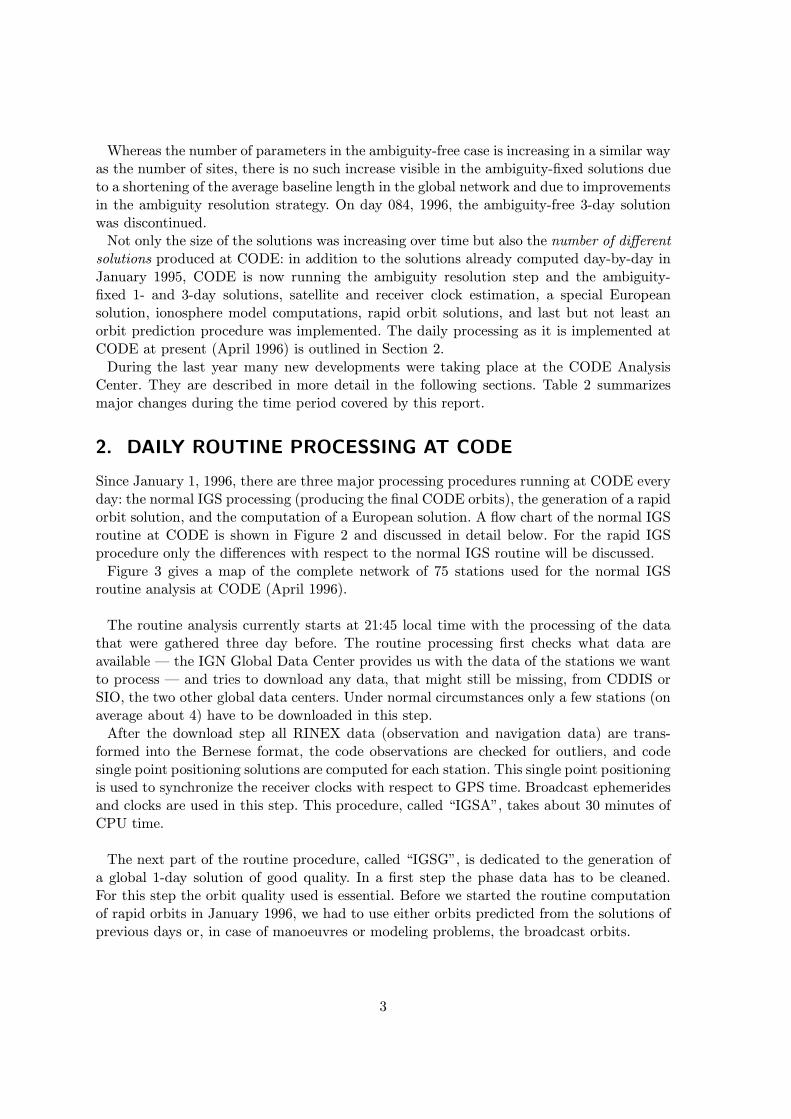
Since January 1, 1996, there are three major processing procedures running at CODE everyday: the normal IGS processing (producing the final CODE orbits), the generation of a rapidorbit solution, and the computation of a European solution. A flow chart of the normal IGSroutine at CODE is shown in Figure 2 and discussed in detail below. For the rapid IGSprocedure only the differences with respect to the normal IGS routine will be discussed.Figure 3 gives a map of the complete network of 75 stations used for the normal IGS

routine analysis at CODE (April 1996).

The routine analysis currently starts at 21:45 local time with the processing of the datathat were gathered three day before. The routine processing first checks what data areavailable — the IGN Global Data Center provides us with the data of the stations we wantto process — and tries to download any data, that might still be missing, from CDDIS orSIO, the two other global data centers. Under normal circumstances only a few stations (onaverage about 4) have to be downloaded in this step.After the download step all RINEX data (observation and navigation data) are trans-

formed into the Bernese format, the code observations are checked for outliers, and codesingle point positioning solutions are computed for each station. This single point positioningis used to synchronize the receiver clocks with respect to GPS time. Broadcast ephemeridesand clocks are used in this step. This procedure, called “IGSA”, takes about 30 minutes ofCPU time.

The next part of the routine procedure, called “IGSG”, is dedicated to the generation ofa global 1-day solution of good quality. In a first step the phase data has to be cleaned.For this step the orbit quality used is essential. Before we started the routine computationof rapid orbits in January 1996, we had to use either orbits predicted from the solutions ofprevious days or, in case of manoeuvres or modeling problems, the broadcast orbits.

3

Date Year/Doy Description of Change at CODE Section01-JAN-95 001/95 Change from the ITRF92 to the ITRF93 coordinate

and velocity set for the 13 fixed sites.3

19-MAR-95 078/95 Pseudo-stochastic pulses set up for the eclipsingsatellites at 45 minutes after the exit from theshadow.

4

04-JUN-95 155/95 Estimation of pseudo-stochastic pulses for all satel-lites at 12:00 UT and 24:00 UT (once per revolution).

4

04-JUN-95 155/95 Submission of the first weekly coordinate solution inthe SINEX format.

3

25-JUN-95 176/95 Ambiguity-fixed solutions submitted as the officialsolution.

8

10-SEP-95 253/95 Precise satellite clocks are estimated using code ob-servations and submitted together with the preciseorbit files.

5

03-NOV-95 307/95 Station GOLD (Goldstone) not fixed any longer onITRF coordinates (unknown antenna change).

3

01-JAN-96 001/96 Routine computation of global ionosphere models tosupport the ambiguity resolution algorithm. Dailyglobal ionosphere models are available starting Janu-ary 1, 1995 (reprocessing of 1995).

7

01-JAN-96 001/96 Computation of the first rapid orbits with a delayof 12 hours after the observations. These orbits arepredicted for two days to obtain real-time orbits.

4

12-JAN-96 012/96 Terrible disk crash. –22-JAN-96 022/96 The new radiation pressure model with 9 paramet-

ers per satellite implemented in processing, but allparameters constrained to zero with the exception ofthe conventional ones (direct rad. pressure coeff. andy-bias). Switch from the Rock4/42 S-model to theT-model.

4

24-MAR-96 084/96 Ambiguity-free 3-day solution discontinued. –24-MAR-96 084/96 Set-up of subdaily pole and UT1-UTC estimates (off-

sets and drifts in 2 hour intervals) in the routinesolutions for internal purposes.

6

07-APR-96 098/96 A routine test solution making use of the fully newradiation pressure model (except that no x-comp. isestimated).

4

07-APR-96 098/96 A special pole file is created using the rapid poleresults to omit large jumps when passing from oneBulletin A file to the next updated version.

–

08-APR-96 099/96 Pseudo-stochastic pulses are set up for all satellites at12:00 UT for the 1-day solutions to improve the orbitquality. These 1-day orbits are used for ambiguityfixing.

4

09-APR-96 100/96 Rapid orbits are computed with fixed ambiguities. 4

Table 2. Changes/Modifications of Processing at the CODE Analysis Center of the IGSDuring 1995 and the Beginning of 1996

4

Outlier removal

Baselinecheck

Iteration

ClockEstimation60 min

30 min

30 min

30 min

60 min

30 min

1-Day

Ionosphere Model

Solution

1-Day Amb. Fix

(G1)

Solution(Q1)

preprocessing

Ambiguity Fixing

60 min

30 min

Data transfer

3-DaySolutions

(S3,R3,X3,C3)

Code preprocessing

Phase

60 min

Figure 2. IGS Data Processing Flow at CODE (April 1996).

In both cases it was necessary to perform an iteration to improve the orbit quality (pro-ducing a first 1-day solution and then cleaning the phase data a second time with theseimproved 1-day orbits). Nowadays such an iterative procedure is obsolete because of thehigh quality of the rapid orbits (manoeuvres have to be dealt with now at the rapid orbitstage). In the 1-day solution (computed after the phase cleaning) we estimate orbit para-meters, ERPs (including ERP drifts), station coordinates, and troposphere zenith delays.Because under AS some receivers (mainly Rogues and some Turborogues) are sometimes

producing data with strange systematic biases that are difficult to detect with our conven-tional pre-processing algorithms, an extra step was added to screen the post-fit residualsof all baselines for outliers. The full 1-day solution is then repeated producing the final1-day results, labeled G1 (see “Global Solution Types” below). The final 1-day orbits havea quality already comparable to the orbits of the best IGS AC centers, but an improvementis still possible when going to longer arcs, i.e. to 3-day solutions.The G1-products are made available on our anonymous ftp account as soon as they have

been computed (see “Daily Products” below).

5

Figure 3. The Global Network of 75 Stations Used in the CODE Routine Analyses.

The complete “IGSG” routine requires about 2.5 hours of CPU time.

The procedure for the 3-day solutions starts with the computation of a global ionospheremodel used for the ambiguity resolution step to follow (see Section 7 and 8). After ambigu-ity fixing (on the single baseline level) a new, complete 1-day solution is generated savingthe normal equation information for all parameters that might be of interest later on (ase.g. the parameters of the extended orbit model, subdaily ERPs, nutation drifts, center ofmass coordinates, satellite antenna offsets, ...). A 3-day solution is then produced combin-ing the normal equations of this last day with the normal equations of the previous two1-day solutions (see [Beutler et al., 1996] for the algorithms used to combine 1-day arcs into3-day arcs). Four different 3-day solutions are currently created in this way, labeled S3, R3,X3, and C3 (see ”Global Solution Types” below). Our official IGS products stem from themiddle day of the R3-solution. The 3-day solution procedure takes about 3 hours CPU time.

Finally a clock solution is computed where the satellite and station clocks are solved forsimultaneously using code observations only. This clock solution is described in detail inSection 5 and takes about 1 hour of CPU time including one iteration and several steps forquality checks.The complete IGS routine needs about 7 hours of CPU time per day, which means about

10 hours turn-around time.

6

The Rapid Orbit Computation

Since January 1, 1996, CODE is making available rapid orbits with a delay of only 12hours! The estimation scheme for the rapid orbits is very similar to the normal routineprocessing up to the 1-day ambiguity-fixed solution. The basic differences are that (a)an iteration is necessary for the orbit improvement, since there is no good a priori orbitinformation available, and that (b) at present no ionosphere model is estimated and used inthe ambiguity resolution step. The final rapid orbit solution is a 5-day solution with 5-daysatellite arcs in contrast to the 3-day arcs in the normal procedure. For these 5-day solutionsthe 9 radiation pressure parameters of the extended orbit model are set up and solved for.The most important difference from the operational point of view is, however, that the

rapid orbits are generated using the Bernese Processing Engine (BPE), a tool for the fullyautomated processing of permanent networks, which allows a parallel processing on manyCPUs. The ambiguity resolution step e.g., which is done baseline by baseline, is run on 6different machines simultaneously. This reduces the processing time considerably becauseit makes optimal use of the 6 DEC Alpha stations available at our university. Instead of10 hours (normal IGS procedure) the generation of the rapid orbits takes about 3 hoursturn-around time. With such a strategy the processing time only grows linearly with thenumber of stations, i.e. a network of about 100 stations might be processed in 4 hours.

The European Solution

Apart from the normal and the rapid IGS procedures CODE also generates a Europeansolution. This solution — Figure 4 shows a map of the network — is computed with a delayof about 2 weeks making use of the official CODE products (orbits and ERPs).

Figure 4. European Network of 35 Stations Processed at CODE with a Delay of two Weeks.

7

It was mainly set up for test purposes. With this regional network we can in a first stepcheck the quality of our orbits, then use it to test new processing strategies, and finallygain experiences in how a typical IGS “customer” should make use of the IGS products toachieve the highest possible precision and how the regional solutions may be combined withthe global solutions (densification issues).The stations CAGL, EBRE, HFLK, PENC, KELY, KIRU, MEDI, NOTO, SFER, VILL, and

ZWEN are included only in this European solution providing an independent check of ourorbit quality, whereas all other sites are also part of the global CODE solution.The series of European solutions is combined with the series of global solutions for the

annual submission to the ITRF Sub-bureau of the IERS.

Global Solution Types

Several different solution series are routinely generated at the CODE Analysis Center (seealso Figure 2), although only one official series is submitted to the global data centers:

G1-Series: Since June 21, 1992, our final 1-day solution. Precise ephemerides files, earthrotation parameters, and station coordinates are saved. The orbits and ERPs areavailable on our anonymous ftp account until we have completed our official 3-daysolution. Older results are available on request.

Q1-Series: Q1 designates the ambiguity-fixed 1-day solution series. Although the compu-tation of Q1-solution started on June 25, 1995, we began only recently to save theresults of this solution type.

R3-Series: Starting June 25, 1995 (GPS week 807), this is the official CODE solution de-livered to the global data centers. The satellites are modeled using our conventional8 parameter orbit model. In addition, five small velocity changes (pseudo-stochasticpulses) per satellite are estimated over the 3-day arc in the radial and along-track di-rections. The earth orientation parameters are estimated as a first degree polynomialover the three days. Four troposphere zenith delays are determined per station andday.

S3-Series: The S3-series only started on April 7, 1996. But due to the reprocessing of 1995(including S3-solutions) almost a full year of S3-solutions is available. The S3-series isidentical to the R3-series with the exception of the ERP estimation: instead of one firstdegree polynomial over three days we estimate subdaily pole and UT1-UTC values in2-hour intervals (see Section 6).

X3-Series: This solution type was started together with the S3-series on April 7, 1996, andwas also included in the reprocessing of 1995. This solution determines a subset of theparameters of the extended orbit model (the “X”-terms are heavily constrained, seeSection 4). Apart from this the X3-series is identical to the R3-series.

C3-Series: This series is produced since January 1, 1994. It includes the estimation of thenutation drift corrections in longitude ∆ψ and obliquity ∆ε (in addition to the otherERPs). All other characteristics are identical to the R3-Series (except that beforeApril 7, 1996, the C3-series was based on ambiguity-free solutions).

8

Daily Products

On the anonymous ftp account CODE makes available several of its (IGS) products (ftpubeclu.unibe.ch -or- 130.92.6.11, after login: cd aiub$ftp).The anonymous ftp area is divided into two product directories: the directory CODE con-

taining our official IGS products and the Bernese Software user directory BSWUSER withBernese-specific information like daily coordinates and troposphere estimates.

BSWUSER --- ATM CODE --- 1992

|-- DATPAN |-- 1993

|-- GEN |-- 1994

|-- OUT |-- 1995

|-- STA

The subdirectories of the CODE directory contain the products of the past years. Some of theproducts in these annual directories have been compressed using the standard compressionalgorithms used by the IGS (e.g. for RINEX file compression). The data of the currentyear is located (in uncompressed form) directly in the CODE directory. A summary of theproducts available on our anonymous ftp is given in Table 3.

Daily ProductsCODwwwwd.EP1 CODE 1-day orbits (G1-series). Available with a 3-day delayCODwwwwd.ER1 CODE 1-day ERPs (G1-series) belonging to the 1-day orbitsCODwwwwd.ERH_R CODE rapid orbits. Available with a 12-hour delayCODwwwwd.ERP_R CODE rapid ERPs belonging to the rapid orbitsCODwwwwd.EPH_P CODE 24-hour orbit predictionsCODwwwwd.ERH_P2 CODE 48-hour orbit predictions

Weekly ProductsCODwwwwd.EPH CODE final orbits (R3-series). This is our official orbit product!CODwwwwd.ERP CODE final ERPs (R3-series) belonging to the final orbitsCODwwww7.SUM CODE weekly summary fileCODwwww7.SNX CODE weekly SINEX fileCODwwwwd.ION CODE daily global ionosphere model, Bernese formatCODwwwwd.CLK CODE satellite clock estimates (5 min. sampl.), Bernese formatB1_yyddd.CLK Broadcast satellite clock information, Bernese format

BSWUSER SubdirectoriesATM Contains the troposphere estimates of the R3-seriesDATPAN Contains some files specific to the Bernese softwareGEN Official IERS poles (C04 and Bulletin A) in the Bernese format

and some additional files for the Bernese softwareOUT Contains the ERP estimates of the R3-seriesSTA Contains the coordinate estimates of the R3- and the European

series

Table 3. CODE Products Available Through Anonymous FTP.

9

3. COORDINATES AND VELOCITIES

With the beginning of the year 1995 the CODE Analysis Center introduced, in agreementwith all other Analysis Centers of the IGS, the ITRF93 (IERS Terrestrial Reference Frame)as the new reference for the computation of the daily products (orbits and ERPs). Thesystem is realized by tightly constraining the coordinate and velocity values of the 13 IGScore sites to the ITRF93 values in the daily solutions.A consequence of the change from ITRF92 to ITRF93 is a discontinuity in the x- and

y-coordinates of the pole; the LOD estimates are not affected. Based on normal equationswe reprocessed all the solutions back to September 1993 to determine the impact of thesystem change [Brockmann, 1996]. A comparison of the two series (ITRF92 and ITRF93 asreference frame) over a time interval of about 1.5 years gives the following results:At epoch 1993.0 we see an offset in the x- and y-pole of about -0.15 ± 0.06 mas and -0.85± 0.08 mas respectively. The drift difference of -0.45 ± 0.06 mas/yr in the x-pole and -0.40± 0.05 mas/yr in the y-pole can be attributed to the differences between the two velocityfields (alignment with NNR-NUVEL1 for ITRF92 versus alignment with the C04 pole driftfor ITRF93).

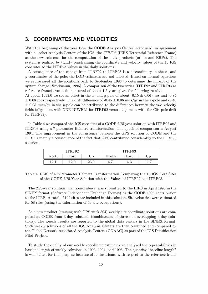
In Table 4 we compared the IGS core sites of a CODE 2.75-year solution with ITRF92 andITRF93 using a 7-parameter Helmert transformation. The epoch of comparison is August1994. The improvement in the consistency between the GPS solution of CODE and theITRF is mainly a consequence of the fact that GPS contributed considerably to the ITRF93solution.

ITRF92 ITRF93

North East Up North East Up

12.1 12.0 23.9 4.7 4.3 11.7

Table 4. RMS of a 7-Parameter Helmert Transformation Comparing the 13 IGS Core Sitesof the CODE 2.75-Year Solution with the Values of ITRF92 and ITRF93.

The 2.75-year solution, mentioned above, was submitted to the IERS in April 1996 in theSINEX format (Software Independent Exchange Format) as the CODE 1995 contributionto the ITRF. A total of 102 sites are included in this solution. Site velocities were estimatedfor 58 sites (using the information of 69 site occupations).

As a new product (starting with GPS week 804) weekly site coordinate solutions are com-puted at CODE from 3-day solutions (combination of three non-overlapping 3-day solu-tions). The weekly results are reported to the global data centers in the SINEX format.Such weekly solutions of all the IGS Analysis Centers are then combined and compared bythe Global Network Associated Analysis Centers (GNAAC) as part of the IGS DensificationPilot Project.

To study the quality of our weekly coordinate estimates we analyzed the repeatabilities inbaseline length of weekly solutions in 1993, 1994, and 1995. The quantity ”baseline length”is well-suited for this purpose because of its invariance with respect to the reference frame

10

definition. The velocities estimated from 2.75 years of GPS observations were used to takeinto account the linear motion of the sites within the time period analyzed.Assuming that the baseline length repeatability σL may be written as a linear function of

the baseline length L:

σL [mm] = a [mm] + b [ppb] · L [1000 km]. (1)

we obtain the values listed in Table 5 for the three years.

Year # Baselines Repeatability(Interval) (# Stations) a [mm] b [ppb]

1993 383(0.75 yrs) 33

0.09 2.96

1994 520(1.0 yrs) 44

1.07 2.00

1995 765(1.0 yrs) 65

1.77 1.41

Table 5. Repeatability for the Baseline Length Determined from Weekly Free GPS Solu-tions.

Substitution of these values into formula (1) shows that a mean precision of 3 mm inbaseline length may be expected for e.g. typical baselines in Europe of 1000 km using oneweek of continuous GPS observations. A considerable improvement from 1993 to 1995 can beseen for long baselines. A 6000 km baseline (e.g. between Europe and North America) wasdetermined with a precision of approximately 18mm in 1993 and with about 10mm in 1995.The improvement in the results is mainly a consequence of the increasing number of globalIGS sites, the better geographical distribution, and the improvements in the processingstrategies at the CODE Analysis Center.The excellent agreement between the weekly results of different Analysis Centers is demon-

strated by the IGS reports of the three Global Network Associated Analysis Centers and isnot discussed here.In Figure 5 we would like to address the problem of the station height estimation in the

case of a mixture of different antenna types.

Figure 5. Comparison of Station Height Estimates for the Site JOZE Derived from theWeekly SINEX Contributions of the IGS Analysis Centers.

11

Depending on how elevation-dependent antenna phase center variation are modeled, largedifferences may be seen between the height estimates of the individual IGS Analysis Centers(see Section 9). The reason of the discrepancy between the CODE heights on one hand andthe SIO heights on the other hand resdies in the fact that SIO does not apply elevation-dependent phase center variations for the Trimble antennas (relative to the Dorne Margolinantennas).

4. ORBIT MODELING IMPROVEMENTS

During the first months of 1995 it became more and more evident that the orbit model usedat CODE was not sufficient to represent the satellite trajectories over a 3-day period, evenfor satellites not passing through the Earth shadow. Figure 6 compares five different orbitestimation strategies

1. 1-day arcs without the estimation of pseudo-stochastic pulses

2. 1-day arcs with 2 stochastic pulse per revolution (one in radial “R”, the other inalong-track direction “S”)

3. 3-day arcs without pseudo-stochastic pulses

4. 3-day arcs with 2 stochastic pulses per revolution

5. 3-day arcs with 3 stochastic pulses per revolution (including an additional pulse perrevolution in the out-of-plane direction “W”)

by fitting a 7-day arc through 7 individual 1-day or 3-day solutions (middle days only)using the CODE Extended Orbit Model (9 radiation pressure parameters instead of 2, see[Beutler et al., 1994]). The improvement due to the estimation of pseudo-stochastic pulsesis pronounced in the case of 3-day solutions.Seeing this, the estimation strategy for pseudo-stochastic pulses was changed on June 4,

1995 (see also Table 2): whereas up to this date pseudo-stochastic pulses were only set up forthe eclipsing satellites, such pulses were now estimated for all satellites. This new strategyconsiderably improved the CODE orbit quality.

In January 1996 the Extended CODEOrbit Model with a maximum of 9 radiation pressureparameters per satellite and arc — only used so far with satellite positions as pseudo-observations (e.g. in the long arc comparisons done by the Analysis Center Coordinator)— was fully implemented into the parameter estimation and normal equation stackingprograms [Springer et al., 1996]. The full radiation pressure model may now be estimatedusing the phase (and code) observations directly. The final CODE products are still basedon the conventional radiation pressure model, although all 9 radiation pressure parametersare set up for later use.Reprocessing about 8 months of the year 1995 with the Extended CODE Orbit Model

gave us a sufficiently long series of solutions to obtain more information on how this newmodel may be optimally tuned for the routine CODE processing.

12

Figure 6. Comparison of Orbit Estimation Strategies by fitting a 7-Day Arc Trough the7 individual 1- or 3-day solutions of GPS Week 765 Using the Extended CODEOrbit Model.

The new model is already in daily use for two other IGS applications at CODE thatstarted in January 1996: the rapid orbit determination and the orbit predictions.The rapid orbit procedure used at CODE has already been described in Section 2 and the

quality of this new product — available 12 hours after the observations — may be seen inthe weekly IGS reports of the rapid orbit combination. In the orbit prediction scheme therapid orbit results from the last three days are fitted using 3-day arcs. These arcs are thenextrapolated for two days thus making predicted orbits available for real-time applications.The quality presently achieved is about 30 cm for 1-day predictions and about 80 cm for 2-day predictions (needed for real-time applications). Both products (the CODE rapid orbitsand the orbit predictions) are available at CODE since January 1, 1996 (see Table 3).

During the last year some research was performed at CODE concerning the correlationsbetween ERPs and orbital parameters with the goal to improve the quality and stability ofthe UT1-UTC and nutation drifts determined from global GPS data. First results concerningthe correlation between UT1-UTC, the pseudo-stochastic pulses, and the conventional tworadiation pressure parameters (direct coeff. and y-bias) were presented in [Rothacher et al.,1995c]. A more general approach (including also nutation parameters) may be found in[Rothacher et al., 1996].

5. SATELLITE CLOCK ESTIMATION

Since September 10, 1995 (GPS week 818) precise satellite clocks are routinely determinedat CODE and reported to the IGS global data centers in the precise orbit format. The

13

procedure to estimate the satellite and station clocks is the last part of our IGS routineprocessing. It consists of five steps.First a reference clock has to be selected because not all (receiver and satellite) clocks

can be estimated. We normally use the receiver clock at Algonquin as time reference. If theAlgonquin data are not available another station connected to a hydrogen maser frequencystandard is automatically selected. This reference clock is then aligned to GPS time byestimating offset and drift with respect to the broadcast satellite clock values.In the second step, the actual clock estimation, all good code observations are processed

simultaneously to estimate all satellite and station clocks except the clock of the selectedreference station. We currently use code measurements only (no phase observations) andonly from receivers which are not affected by AS-related biases in the code observations.No Rogue receivers, but most of the Turborogue and all Trimble receivers are included. Forthe clock estimation we use our “final” orbits, ERPs and coordinate results to guaranteethat the clock estimates are consistent with the other final CODE products.The estimated satellite clocks are then used in the third step to compute a code single

point positioning solution for each station contributing to the clock estimation. This aloowsus to detect and remove outliers and, if necessary, to repeat the actual clock estimation.A similar single point positioning solution (step 4) — estimating only offset and drift for

each receiver clock instead of epoch-wise clock corrections — allows us check whether thereference clock had a jump sometime during the day and shows us which stations have goodexternal oscillators connected to the GPS receivers.In the fifth and last step a code single point positioning, but now using all available code

data (including the data from stations with code biases), is done to verify the code qualityof all receivers. In this last step we use a cut-off angle of 20 degrees. In all other steps thecut-off angle is set to 30 degrees to avoid the effects of code multipath.The quality of the CODE satellite clock estimates is of the order of 1-2 nsec (according to

the weekly reports on IGS orbit combination, where the satellite clock results are combinedand compared, too).

6. EARTH ROTATION PARAMETERS AND NUTATION

The quality of the daily ERP values obtained from the CODE 3-day solutions is now of theorder 0.1–0.2 mas for the x- and y-pole components and about 0.02 msec for LOD. Thiscan be seen from the monthly and weekly IGS reports of the IERS Central Bureau andIERS Rapid Service Sub-bureau.

At CODE we are also routinely estimating — in the special solution series C3 (see Section2) — the drifts of the nutation in longitude ∆ψ and obliquity ∆ε. The a priori nutationmodel introduced for all the global CODE solutions is the IAU 1980 model, i.e. no correctionterms as e.g. given in [McCarthy, 1995] are taken into account. The estimated nutation driftsare therefore corrections with respect to the IAU 1980 model. A series of such nutation driftsis available from April 22, 1994, up to now, covering a time interval of almost two years. Itis clear that GPS cannot contribute to the long-periodic nutation terms, but it might givecontributions to a future nutation model in the high frequency domain. As examples thespectra obtained from the daily estimated nutation drifts in obliquity and in longitude areshown here in Figure 7 covering periods from 3 to 12 days.

14

0

0.5

1

3 3.5 4 4.5 5 5.5 6

Period in Days

Pow

er s

pect

ral d

ensi

tySpectrum of Nutation Drifts in Obliquity

0

0.5

1

6 7 8 9 10 11 12

Period in Days

Pow

er s

pect

ral d

ensi

ty

Spectrum of Nutation Drifts in Obliquity

0

0.5

1

3 3.5 4 4.5 5 5.5 6

Period in Days

Pow

er s

pect

ral d

ensi

ty

Spectrum of Nutation Drifts in Longitude

0

0.5

1

6 7 8 9 10 11 12

Period in Days

Pow

er s

pect

ral d

ensi

ty

Spectrum of Nutation Drifts in Longitude

Figure 7. Spectrum of Nutation Corrections in Obliquity and Longitude Derived From theCODE Results in the Time Interval from April 1994 to January 1996.

15

The dotted vertical lines mark the known nutation periods (e.g. given in the IERS Stand-ards [McCarthy, 1992]). In a next step the nutation drift series will be analysed to obtainthe amplitudes of the most important correction terms that may then be compared to the-oretical and VLBI-derived models. A first GPS nutation model was presented at the XXI.General Assembly of the IUGG in Boulder [Weber et al., 1995].After having processed several time periods (CONT’94 and CONT’95 campaigns, and a

3-month period in fall 1995) with the estimation of subdaily ERPs for test purposes, weare now routinely setting up ERPs (pole x- and y-coordinates, and UT1-UTC) in 2-hourbins, i.e. as a linear function over 2 hours, enforcing continuity at the interval boundaries.For the official CODE results, these 2-hourly parameter sets are reduced to just one setover the three days of a 3-day solution. At present no a priori model for the subdaily ERPvariations is included in the CODE solutions and the results reported to the IERS andIERS Sub-bureau are not containing any subdaily corrections . (The values reported fornoon each day are the mean values over one day averaging the subdaily variations).Based on the saved daily normal equation systems a special solution — called S3 in

Figure 2 — is produced to estimate the subdaily variations. This S3-series was started onMarch 22, 1996. Thanks to the reprocessing effort the same solution type (S3) is availablefor all days since day of year 127 in 1995. This time series should allow a detailed study ofthe subdaily ERP variations that can be obtained from a global GPS network. First resultswere presented by [Weber et al., 1995] and [Springer et al., 1995].

7. GLOBAL IONOSPHERE MAPPING

As shown in [Schaer et al., 1995] it is possible to produce reasonable Global IonosphereMaps (GIMs) by analyzing of the geometry-free linear combination of double-differencephase observations. We are fully aware of the fact that by using double instead of zerodifferences we loose part of the ionospheric signal, but we have the advantage of clean ob-servations (no code biases). In addition we are not affected by Anti-Spoofing (AS).

Since January 1, 1996 (see Table 2 and Figure 2), the GIM estimation procedure is runningin an operational mode. Several GIM products are computed every day:

• Ambiguity-free 1-day GIMs are estimated right prior to the ambiguity resolution step.These GIMs are subsequently used to improve the resolution of the initial carrier phaseambiguities on baselines up to 2000 kilometers.

• Improved GIMs (ambiguity-fixed, with single-layer heights estimated) are derived afterthe ambiguity resolution step.

At present, the GIM files containing the TEC coefficients for one day are available with adelay of 4 days. These files are copied weekly to our anonymous ftp server.The global TEC distribution is represented over 24 hours by spherical harmonics up to

degree 8 in a geographical reference frame which is co-rotating with the mean Sun. A single-layer model is adopted in this approach assuming a spherical ionospheric shell in a heightof 400 kilometers above the Earth’s mean surface. To extract the global TEC informationa separate least-squares adjustment of the observations of the complete IGS network isperformed using an elevation cut-off angle of at present 20 degrees. Note that — even under

16

AS— no restrictions concerning receiver types or satellites have to be made in our approach.An example of a 1-day GIM representing an average TEC distribution is shown in Figure 8.

−180 −135 −90 −45 0 45 90 135 180−90

−60

−30

0

30

60

90

2 2

2

2

4

4

4

4

6

6

6

6

8

8

10

10

12 12

12

14

14

16

16

18

20

22 24

26

28

30

32 34

Vertical Total Electron Content in TECU

Sun−fixed longitude in degrees

Latit

ude

in d

egre

es

Figure 8. Global Ionosphere Map (GIM) for Day 073, 1996, Plotted in a Sun-Fixed Co-ordinate System.

After reprocessing all IGS data of the year 1995 and gathering all GIMs already pro-duced in 1996, we may present a long-time series of global TEC parameters [Schaer et al.,1996]. Two special TEC parameters, namely the maximum and the mean TEC, roughlycharacterizing the deterministic part of the ionosphere, are shown in Figure 9.

0 50 100 150 200 250 300 350 400 4500

20

40

60

80

Time in days since January 1, 1995

Max

and

mea

n T

EC

in T

EC

U

Figure 9. Maximum and Mean TEC Values Extracted from the Daily CODE GIMs

17

The three non-AS periods in 1995 are marked by dashed lines.Let us mention that we also generate regional ionosphere maps for Europe based on about

30 European IGS stations in a fully automatic mode since December 1995. These ionospheremaps are used in the processing scheme of the European cluster to support the ambiguityresolution there. The European TEC maps are available on special request.

8. GLOBAL AMBIGUITY RESOLUTION

Since June 25, 1995 (GPS week 807) — after an experimental phase of several months —the ambiguity-fixed 3-day solutions are submitted to the IGS as official CODE contribution.We perform ambiguity resolution on baselines up to 2000 kilometers using the so-calledQuasi-Ionosphere-Free (QIF) ambiguity resolution strategy [Mervart, 1995], which allowsambiguity resolution on long baselines without using code measurements. Since January 1,1996, the QIF strategy is supported by GPS-derived global ionosphere models [Schaer et al.,1996]. At present we resolve about 85% of the ambiguities referring to baselines below2000 kilometers, that means that on average about 50% of all ambiguities can be fixed ontheir integer values (see also Figure 1). Figure 10 shows the percentage of resolved ambiguityparameters on baselines shorter than 2000 kilometers. We may recognize (a) three significantpeaks caused by AS-free periods and (b) on January 1, 1996, a jump of about 10% whenwe started to use our 1-day GIMs.

45

50

55

60

65

70

75

80

85

90

0 50 100 150 200 250 300 350 400 450 500

Num

ber

of A

mbi

guiti

es F

ixed

(%

)

Day of year 1995

Figure 10. Percentage of Ambiguities Fixed on Baselines Below 2000 km.

The effect of resolving ambiguities in a global network has been discussed in [Mervartet al., 1995].

18

9. ANTENNA PHASE CENTER CALIBRATIONS

The importance of the antenna phase center calibrations for the IGS network can be seenfrom the example given in Section 3, Figure 5.During the last year two GPS antenna calibration campaigns were processed at the AIUB

to compute elevation-dependent phase center variations:

• The THUN-94 Campaign

• The WETTZELL-95 Campaign

The antenna types calibrated during these campaigns were DORNE MARGOLIN T and B

(Turborogue, Rogue), 4000ST L1/L2 GEOD (SN14532, Trimble), TR GEOD L1/L2 (SN22020,Trimble), SR299E EXTERNAL and SR299 INTERNAL (Leica), and GEOD L1/L2 P (SN700228,Ashtech).The results show that the phase center variations estimated from GPS data are very

consistent, even between different campaigns with different local environments (multipath).For the L1 frequency the agreement between the GPS results and the results of recent

UNAVCO chamber tests [Rocken et al., 1996] is very promising, not so, however, for the L2results, where some problems still wait for a solution.The estimation strategy, the models used, and results have been published in [Rothacher

et al., 1995b], [Rothacher et al., 1995a], and [Rothacher and Schaer, 1996].The elevation-dependent phase center corrections used in the CODE processing are listed

in Table 6.

PHASE CENTER OFFSETS INCLUDING ELEVATION DEPENDENCE USED AT CODE

----------------------------------------------------------------------------------------------------

RECEIVER TYPE FREQ PHASE CENTER OFFSETS (M) ELEVATION DEPENDENCE OF PHASE CENTER (MM)

ANTENNA TYPE L* NORTH EAST UP 90 85 80 75 70 65 60 55 50 45 40 35 30 25 20 15 10

****************** * **.**** **.**** **.**** ** ** ** ** ** ** ** ** ** ** ** ** ** ** ** ** **

ROGUE SNR-8 1 0.0 0.0 0.0779 0 0 0 0 0 0 0 0 0 0 0 0 0 0 0 0 0

DORNE MARGOLIN B 2 0.0 0.0 0.0964 0 0 0 0 0 0 0 0 0 0 0 0 0 0 0 0 0

ROGUE SNR-8 1 0.0 0.0 0.0779 0 0 0 0 0 0 0 0 0 0 0 0 0 0 0 0 0

DORNE MARGOLIN R 2 0.0 0.0 0.0964 0 0 0 0 0 0 0 0 0 0 0 0 0 0 0 0 0

ROGUE SNR-8100 1 0.0 0.0 0.1100 0 0 0 0 0 0 0 0 0 0 0 0 0 0 0 0 0

DORNE MARGOLIN T 2 0.0 0.0 0.1280 0 0 0 0 0 0 0 0 0 0 0 0 0 0 0 0 0

TRIMBLE 4000SSE 1 0.0 0.0 0.0692 0 1 3 7 10 13 15 16 18 17 16 15 12 11 10 9 8

4000ST L1/L2 GEOD 2 0.0 0.0 0.0677 0 0 2 3 3 4 5 5 7 7 6 7 7 6 7 7 6

TRIMBLE 4000SSE 1 0.0 0.0 0.0625 0 1 3 7 10 13 15 16 18 17 16 15 12 11 10 9 8

TR GEOD L1/L2 GP 2 0.0 0.0 0.0625 0 0 2 3 3 4 5 5 7 7 6 7 7 6 7 7 6

TRIMBLE 4000SSE 1 0.0 0.0 0.0700 -4 -4 -4 -3 -2 -2 -1 0 1 1 1 0 -1 -1 -1 0 8

M-PULSE L1/L2 SUR 2 0.0 0.0 0.0900 -3 -2 0 0 -1 0 0 0 1 1 1 0 1 1 1 1 -5

Table 6. Antenna Phase Center Corrections Used at the CODE Analysis Center Since 1993

The offsets are given relative to the ”Antenna Reference Point” as defined by the IGS(for antenna names and antenna sketches see the files ANTENNA.GRA and RCVR ANT.TAB at

19

the IGS Central Bureau Information System described in [Gurtner and Liu, 1995]). Theelevation-dependent corrections for the Trimble antennas (relative to the Rogue antennas!)were introduced into the routine processing on July 20, 1993, and are stemming from oldchamber measurements by [Schupler et al., 1994], the values for the Trimble micropulseantenna were introduced in April 1996 (for the EBRE site) and were computed at theAIUB from GPS calibration measurements.A new and improved set of consistent calibration values are currently put together from

various sources by a small group and should be implemented by the IGS Analysis Centersby June 30, 1996.

References

Beutler, G., E. Brockmann, W. Gurtner, U. Hugentobler, L. Mervart, and M. Rothacher (1994),Extended Orbit Modeling Techniques at the CODE Processing Center of the International GPSService for Geodynamics (IGS): Theory and Initial Results, Manuscripta Geodetica, 19, 367–386,April 1994.

Beutler, G., E. Brockmann, U. Hugentobler, L. Mervart, M. Rothacher, and R. Weber (1996), Com-bining consecutive short arcs into long arcs for precise and efficient gps orbit determination, Journalof Geodesy, 70, 287–299.

Brockmann, E. (1996), Combination of Solutions for Geodetic and Geodynamic Applications of theGlobal Positioning System (GPS), Ph.D. dissertation, Astronomical Institute, University of Berne,Berne, Switzerland (in preparation).

Gurtner, J., and R. Liu (1995), The Central Bureau Information System, in IGS 1994 Annual Report,edited by R. Liu J.F. Zumberge and R.E. Neilan, pp. 43–57, IGS Central Bureau, Jet PropulsionLaboratory, Pasadena, California U.S.A., September 1 1995.

McCarthy, D.D. (1992), IERS Standards (1992), IERS Technical Note 13, Observatoire de Paris,Paris, July 1992.

McCarthy, D.D. (1995), IERS Standards (1995), IERS Technical Note (in preparation), Observatoirede Paris, Paris, July 1995.

Mervart, L. (1995), Ambiguity Resolution Techniques in Geodetic and Geodynamic Applications ofthe Global Positioning System, Geodatisch-geophysikalische Arbeiten in der Schweiz, Band 53.

Mervart, L., G. Beutler, M. Rothacher, and S. Schaer (1995), The Impact of Ambiguity Resolutionon GPS Orbit Determination and on Global Geodynamics Studies, presented at the XXI. GeneralAssembly of the International Union of Geodesy and Geophysics, Boulder, Colorado, July 2–141995.

Rocken, C., C. Meertens, B. Stephens, J. Braun, T. VanHove, S. Perry, O. Ruud, M. McCallum,and J. Richardson (1996), Receiver and antenna test report, UNAVCO Academic Research Infra-structure (ARI).

Rothacher, M., and S. Schaer (1996), Processing of GPS Antenna Calibration Campaigs at AIUBUsing Double-Difference Phase Observations, presented at the IGS Analysis Center Workshop,NOAA, Silver Spring, USA, March 19–21 1996.

Rothacher, M., W. Gurtner, S. Schaer, R. Weber, W. Schluter, and H.O. Hase (1995a), Azimuth- andElevation-Dependent Phase Center Corrections for Geodetic GPS Antennas Estimated From GPSCalibration Campaigns, in International Association of Geodesy Symposia, Symposium No. 115:GPS Trends in Precise Terrestrial, Airborne, and Spaceborne Applications, edited by G. Beutleret al., Springer, Boulder, CO, USA, July 3–4 1995.

Rothacher, M., S. Schaer, L. Mervart, and G. Beutler (1995b), Determination of Antenna PhaseCenter Variations Using GPS Data, in IGS Workshop Proceedings on Special Topics and New Dir-ections, edited by G. Gendt and G. Dick, pp. 77–92, GeoForschungsZentrum, Potsdam, Germany,May 15–18 1995.

20

Rothacher, M., G. Beutler, and L. Mervart (1995c), The Perturbation of the Orbital Elements of GPSSattelites Through Direct Radiation Pressure, in IGS Workshop Proceedings on Special Topics andNew Directions, edited by G. Gendt and G. Dick, pp. 152–166, GeoForschungsZentrum, Potsdam,Germany, May 15–18 1995.

Rothacher, M., G. Beutler, and T. A. Springer (1996), The Impact of the Extended CODE OrbitModel on the Estimation of Earth Rotation Parameters, presented at the IGS Analysis CenterWorkshop, NOAA, Silver Spring, USA, March 19–21 1996.

Schaer, S., G. Beutler, L. Mervart, M. Rothacher, and U. Wild (1995), Global and Regional Iono-sphere Models Using the GPS Double Difference Phase Observable, in IGS Workshop Proceedingson Special Topics and New Directions, edited by G. Gendt and G. Dick, pp. 77–92, GeoForschungs-Zentrum, Potsdam, Germany, May 15–18, 1995.

Schaer, S., G. Beutler, M. Rothacher, and T.A. Springer (1996), Daily Global Ionosphere MapsBased on GPS Carrier Phasa Data Routinely Produced by the CODE Analysis Center, presentedat the IGS Analysis Center Workshop, NOAA, Silver Spring, MD, USA, March 19–21, 1996.

Schupler, B.R., R.L. Allshouse, and T.A. Clark (1994), Signal Characteristics of GPS User Antennas,Preprint accepted for publication in Navigation in late 1994.

Springer, T.A., G. Beutler, M. Rothacher, and E. Brockmann (1995), The Role of Orbit Modelswhen Estimating Earth Rotation Parameters using the Global Positioning System, presented atthe AGU Fall Meeting, EOS Transactions, 76 (46), 60, November 7 1995.

Springer, T.A., M. Rothacher, and G. Beutler (1996), Using the Extended CODE Orbit Model: FirstExperiences, presented at the IGS Analysis Center Workshop, NOAA, Silver Spring, USA, March19–21 1996.

Weber, R., G. Beutler, E. Brockmann, and M. Rothacher (1995), Monitoring Earth OrientationVariations at the Center for Orbit Determination in Europe (CODE), presented at the XXI.General Assembly of the International Union of Geodesy and Geophysics, Boulder, Colorado, July2–14 1995.

21