Announcement

Lecture on Energy Plus

by Wesley Cole

Monday, December 1, 8 am

ECJ Computer lab

Lecture Objectives:

• Finish with TMY weather data

• Compare detailed and empirical modeling– discus accuracy

• Show how to use life-cycle cost analysis – integrated in eQUEST

TMY weather data

• TMY, TMY2, TMY3• http://rredc.nrel.gov/solar/old_data/nsrdb/1991-2005/tmy3/

1991, 1992, ……………...1994, 1995

TMY3: January , February , March, ….December

Each location - different set

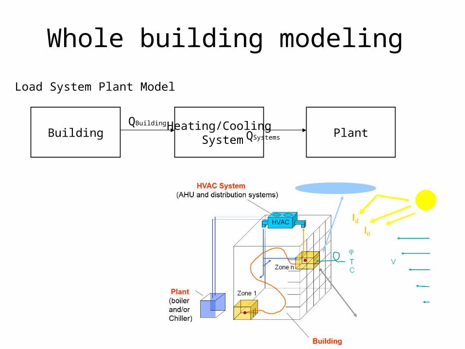
Whole building modeling

BuildingHeating/Cooling

SystemPlant

Load System Plant Model

QBuilding QSystems

Example of System Models:Schematic of simple air handling unit (AHU)

rmSfans

cooler heater

mS

QC QH

wO wS

TR

room TR

Qroom_sensibel

(1-r)mS mS

wM

wR

Qroom_latent

TSTO

wR

TM

Tf,inTf,out

m - mass flow rate [kg/s], T – temperature [C], w [kgmoist/kgdry air], r - recirculation rate [-], Q energy/time [W]

Mixing box

Energy and mass balance equations for Air handling unit model – steady state case

1) The energy balance for the mixing box is:

ROM TrTrT )1( ‘r’ is the re-circulated air portion, TO is the outdoor air temperature, TM is the temperature of the air after the mixing box.

The air-humidity balance for the mixing box is:

ROM wrwrw )1(wO is the outdoor air humidity ratio and

wM is the humidity ratio after the mixing box

2) The energy balance for the cooling coil is given as:

changephaseMSSMSpSCooling iwwmTTcmQ _)(

TOA

water

Building users (cooling coil in AHU)

TCWR=11oCTCWS=5oC

Evaporation at 1oC

T Condensation = TOA+ ΔT

What is COP for this air cooled chiller ?

COP is changing with the change of TOA

Example of Plant Models:Chiller

P electric () = COP () x Q cooling coil ()

Chiller (plant) model: COP= f(TOA , Qcooling , chiller properties)

OACWSOAOACWSCWS TTfTeTdTcTbaCAPTF 12

112

111

CAPFTQ

QPLR

NOMINAL

)(

Chiller data: QNOMINAL nominal cooling power, PNOMINAL electric consumption for QNOMINAL

Cooling water supply Outdoor air

OACWSOAOACWSCWS TTfTeTdTcTbaEIRFT 22

222

222

Full load efficiency as function of condenser and evaporator temperature

PLRcPLRbaEIRFPLR 333

Efficiency as function of percentage of load

Percentage of load:

The coefficient of performance under any condition:

EIRFPLEIRFTCAPFTPP NOMINAL

The consumed electric power [KW] under any condition

)(

)()(

P

QCOP

Available capacity as function of evaporator and condenser temperature

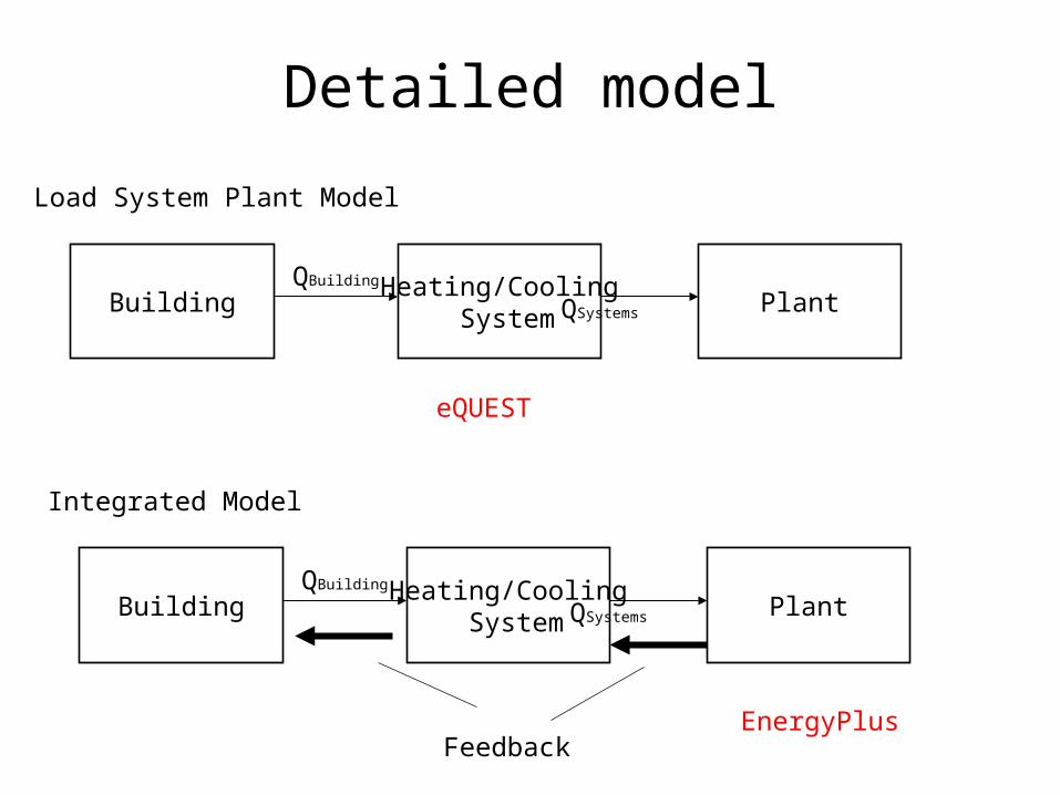
Detailed model

BuildingHeating/Cooling

SystemPlant

Load System Plant Model

QBuilding QSystems

BuildingHeating/Cooling

SystemPlant

Integrated Model

QBuilding QSystems

Feedback

eQUEST

EnergyPlus

Empirical model

5 10 15 20 25 30 35 40 45 50 55 60 65 70 75 80 85 900

50

100

150

200

250

300

350

400

450

500

Q [t

on]

t [F]

Load vs. dry bulb temperature Measured for a building in Syracuse, NY

5 10 15 20 25 30 35 40 45 50 55 60 65 70 75 80 85 900

50

100

150

200

250

300

350

400

450

500

Q=-11.33+1.2126*t

Q=-673.66+12.889*t

Q [t

on]

t [F]

Model

8760

1i ii

ii

57 tif t889.1266.673

57 tif t126.133.11(Q

For an average year use TMY2

=835890ton hour = 10.031 106 Btu

8760

1i ii

ii

57 tif t889.1266.673

57 tif t126.133.11(Q

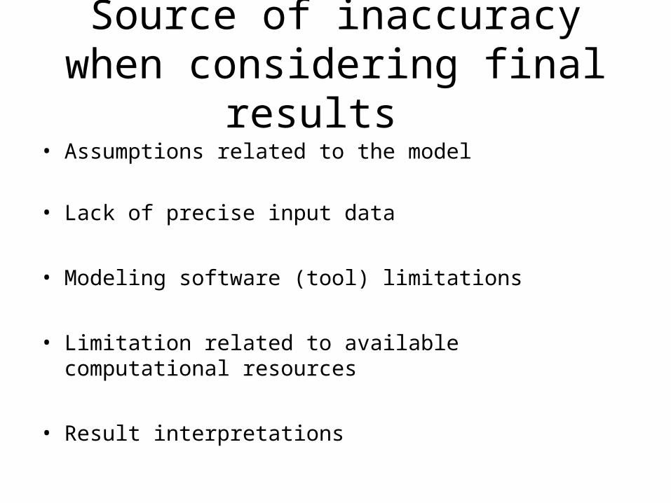
Source of inaccuracywhen considering final results

• Assumptions related to the model

• Lack of precise input data

• Modeling software (tool) limitations

• Limitation related to available computational resources

• Result interpretations

How to evaluate the whole building simulation tools

Two options:

1) Comparison with the experimental data - monitoring

- very expensive- feasible only for smaller buildings

2) Comparison with other energy simulation programs- for the same input data

- system of numerical experiments - BESTEST

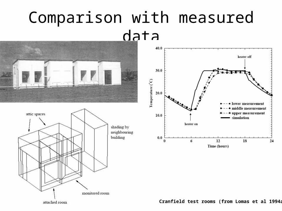
Comparison with measured data

Cranfield test rooms (from Lomas et al 1994a)

BESTEST Building Energy Simulation TEST

• System of tests (~ 40 cases) - Each test emphasizes certain phenomena like

external (internal) convection, radiation, ground contact

- Simple geometry- Mountain climate

6 m

2.7 m

3 m

8 m

0.2 m

0.2 m

1 m

2 m

S

N

E

W

COMPARE THE RESULTS

Example of best test comparison

BESTEST test cases

0

2000

4000

6000

8000

10000

12000

195 200 220 230 240 270

Annual heating load [kWH]

new ES prog

ESP

BLAST

DOE2

SRES/SUN

SRES-BRE

S3PAS

TRYNSYS

TASE

Reasons for energy simulations

• System development

• Building design improvement

• Economic benefits (pay back period)

• Budget planning (fuel consumption)

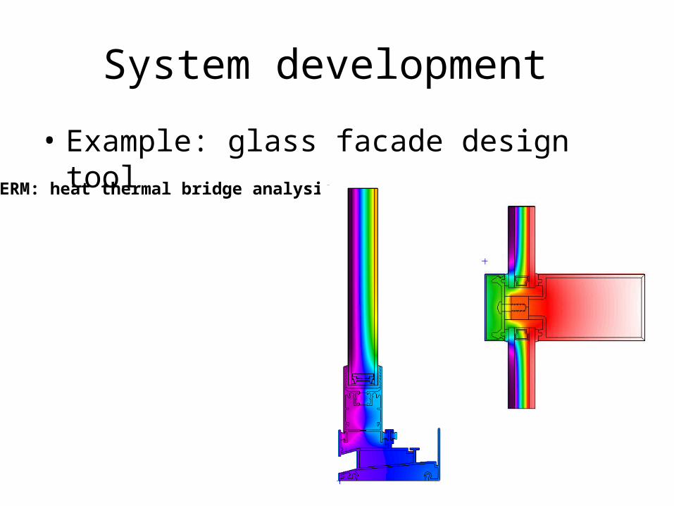
System development

THERM: heat thermal bridge analysis

• Example: glass facade design tool

Building design improvement

• Your projects 1 and 2

Economic benefitsLife Cycle Cost Analysis

• Engineering economics

Energy benefits

Parameters in life cycle cost analysis

Beside energy benefits expressed in $,you should consider:

• First cost• Maintenance• Operation life• Change of the energy cost • Interest (inflation)• Taxes, Discounts, Rebates, other Government

measures

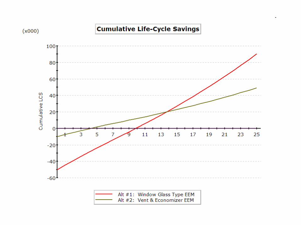
Example

• Using eQUEST analyze the benefits (energy saving and pay back period)

of installing

- low-e double glazed window

- economizer

in the school building in NYC

Reasons for energy simulations

• System development

• Building design improvement

• Economic benefits (pay back period)

• Budget planning (fuel consumption)Least accurate