AnintroductiontoFukayacategories - Université de Nanteschantraine-b/fr/FukayaCategory.pdf · Introduction. This notes serve as a support for a Master2 class given in Universit de

An introduction to Fukaya categories

Baptiste Chantraine

July 15, 2014

2

Introduction.

This notes serve as a support for a Master2 class given in Universit de Nantes in 2014. Theirpurpose do not go beyond this and I have no ambition of giving any news insight into this subject.They are mostly inspired by the better written and more complete book by P. Seidel [Sei08]. Thegoal of the book is to give a definition of the Fukaya category of an exact symplectic manifoldhighlighting the technical details which one might overlook when first work with this concept.Mostly those details concerns the very definition of this A∞-category in particular the definitionof endomorphism spaces. We present here the approach of Seidel to achieve consistent transversedata which are necessary to define this endomorphism space and their composition.

The A∞ equation underlying any A∞-category or algebra is

d∑

i=1

d−i∑

j=0

(−1)zjµd−i+1(ad, ad−1, . . . , aj+i+1, µ

i(aj+i, . . . , aj+1), aj , . . . , a1)= 0 (1)

it reflects the combinatorics of Stasheff’s associahedra. One realisation of these associahedrarelevant in symplectic geometry is Deligne-Mumford’s compactification of pointed Riemann diskswith one positive punctures. In order to achieve consistent perturbation of ∂-equation one needsto decorates this associahedra with perturbation data consistent with this combinatorics. Thiswill occupy Chapters 1 and 3 of the present notes. In Chapter 2 we discuss why those perturba-tions are necessary to have a well defined category.

In Chapter 4 we discuss how to grade the operation µd consistently with the grading of Floertheory and in Chapter 5 we use all those data to define the Fukaya category of an exact symplecticmanifolds and prove that its quasi-equivalence class is independent of all those data.

We then turns our focus on applications of this category to symplectic manifolds and explainsome generation criterion for some of those category 6. This section could occupy a second fullsemester class and we will be here rather quick here. We focus on the most effective criterion

3

4

which is known as Abouzaid’s generation criterion and give an explicit implementation of it forsurfaces.

Contents

1 Deligne-Mumford compactification 7

1.1 Stasheff associahedra. . . . . . . . . . . . . . . . . . . . . . . . . . . . . . . . . . . 7

1.2 Pointed disks . . . . . . . . . . . . . . . . . . . . . . . . . . . . . . . . . . . . . . . 9

1.3 Universal Riemann curve . . . . . . . . . . . . . . . . . . . . . . . . . . . . . . . . 11

1.4 Deligne-Mumford compactification. . . . . . . . . . . . . . . . . . . . . . . . . . . . 11

1.5 Consistent choice of strip-like ends. . . . . . . . . . . . . . . . . . . . . . . . . . . . 13

1.6 Lagrangian labels. . . . . . . . . . . . . . . . . . . . . . . . . . . . . . . . . . . . . 15

2 Naive tentative to define Fukaya category. 17

2.1 Holomorphic curves. . . . . . . . . . . . . . . . . . . . . . . . . . . . . . . . . . . . 17

2.2 Gromov compactness in action. . . . . . . . . . . . . . . . . . . . . . . . . . . . . . 18

2.3 Fukaya categories . . . . . . . . . . . . . . . . . . . . . . . . . . . . . . . . . . . . . 19

3 Perturbed Floer equation and perturbation data. 25

3.1 Floer data. . . . . . . . . . . . . . . . . . . . . . . . . . . . . . . . . . . . . . . . . 25

3.2 Perturbation data . . . . . . . . . . . . . . . . . . . . . . . . . . . . . . . . . . . . 27

5

6 CONTENTS

3.3 Consistent choices of perturbation data. . . . . . . . . . . . . . . . . . . . . . . . . 28

3.4 Linearisation of Equation (3.2) . . . . . . . . . . . . . . . . . . . . . . . . . . . . . 29

4 Grading. 31

4.1 Maslov index. . . . . . . . . . . . . . . . . . . . . . . . . . . . . . . . . . . . . . . . 31

4.2 Graded Lagrangians and dimension of moduli spaces. . . . . . . . . . . . . . . . . . 34

4.3 Index theorem for Cauchy-Riemann operators on the disk. . . . . . . . . . . . . . . 35

4.3.1 Gluing operators . . . . . . . . . . . . . . . . . . . . . . . . . . . . . . . . . 37

4.3.2 Operators over H . . . . . . . . . . . . . . . . . . . . . . . . . . . . . . . . . 37

4.3.3 Proof of the index formula . . . . . . . . . . . . . . . . . . . . . . . . . . . . 37

5 Fukaya categories. 39

5.1 Definition of Fuk(M,ω). . . . . . . . . . . . . . . . . . . . . . . . . . . . . . . . . . 39

5.2 Units . . . . . . . . . . . . . . . . . . . . . . . . . . . . . . . . . . . . . . . . . . . . 40

5.3 Well definedness . . . . . . . . . . . . . . . . . . . . . . . . . . . . . . . . . . . . . 41

5.4 Invariance . . . . . . . . . . . . . . . . . . . . . . . . . . . . . . . . . . . . . . . . . 43

6 Some examples and some generation criterion. 45

6.1 Biran-Cornea’s intersection criterion . . . . . . . . . . . . . . . . . . . . . . . . . . 45

6.2 Toward Abouzaid’s criterion . . . . . . . . . . . . . . . . . . . . . . . . . . . . . . . 46

6.3 Geometric criterion . . . . . . . . . . . . . . . . . . . . . . . . . . . . . . . . . . . . 48

6.4 Example . . . . . . . . . . . . . . . . . . . . . . . . . . . . . . . . . . . . . . . . . . 50

Chapter 1

Deligne-Mumford compactification vs

Stasheff associahedra.

Equation (1) is the algebraic counterpart of the combinatorial description of the faces of a par-ticular family of polyhedra called Stasheff’s associahedra. One of the most fantastic fact is thatthe combinatorics of this family coincide with the combinatorics of a particular compactificationof Riemann disks with punctures on the boundary called Deligne-Mumford compactification (orstable compactification). A second fact not less fantastic than the previous one is that this par-ticular compactification is relevant in the study of symplectic manifold thanks to the celebratedGromov’s Theorem [Gro85] which state that a family of pseudo-holomorphic disks converge (upto semi-stable breaking) to a pseudo-holomorphic map whose domain appears in the Deligne-Mumford compactification.

In this chapter we present first the combinatorics of Stasheff associahedra in terms of default ofassociativity of operations (Section 1.1) then we introduce the space of conformal disks (Section1.2) and describe its stable compactification.

1.1 Stasheff associahedra.

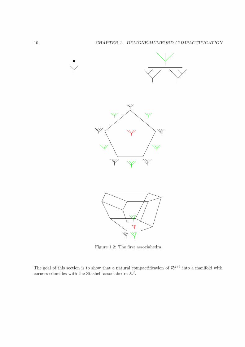
Stasheff associahedra appears in [Sta63] as the polytopes which encodes the non-associativity ofmultiplication in H-space. It is a family of d − 2-dimensional polytopes Kd whose vertices arein bijection with planar rooted tree with d + 1 leaves whose interior vertices have all valence 3(such a tree is called a planar rooted binary tree). Two vertices are connected with one edge if

7

8 CHAPTER 1. DELIGNE-MUMFORD COMPACTIFICATION

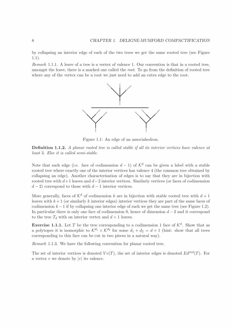
by collapsing an interior edge of each of the two trees we get the same rooted tree (see Figure1.1).

Remark 1.1.1. A leave of a tree is a vertex of valence 1. Our convention is that in a rooted tree,amongst the leave, there is a marked one called the root. To go from the definition of rooted treewhere any of the vertex can be a root we just need to add an extra edge to the root.

Figure 1.1: An edge of an associahedron.

Definition 1.1.2. A planar rooted tree is called stable if all its interior vertices have valence atleast 3. Else it is called semi-stable.

Note that each edge (i.e. face of codimension d − 1) of Kd can be given a label with a stablerooted tree where exactly one of the interior vertices has valence 4 (the common tree obtained bycollapsing an edge). Another characterisation of edges is to say that they are in bijection withrooted tree with d+1 leaves and d−2 interior vertices. Similarly vertices (or faces of codimensiond− 2) correspond to those with d− 1 interior vertices.

More generally, faces of Kd of codimension k are in bijection with stable rooted tree with d + 1leaves with k+1 (or similarly k interior edges) interior vertices they are part of the same faces ofcodimension k− 1 if by collapsing one interior edge of each we get the same tree (see Figure 1.2).In particular there is only one face of codimension 0, hence of dimension d− 2 and it correspondto the tree Td with on interior vertex and d+ 1 leaves.

Exercise 1.1.1. Let T be the tree corresponding to a codimension 1 face of Kd. Show that asa polytopes it is isomorphic to Kd1 × Kd2 for some d1 + d2 = d + 1 (hint: show that all treescorresponding to this face can be cut in two pieces in a natural way).

Remark 1.1.3. We have the following convention for planar rooted tree.

The set of interior vertices is denoted V e(T ), the set of interior edges is denoted Edind(T ). Fora vertex v we denote by |v| its valence.

1.2. POINTED DISKS 9

The root is the 0th leave. All other leaves are numbered counter-clockwise. Each edge going toa leave will have infinite length. The one going to the root will coincide with (−∞,−M) × 0and the one correspond to i-th leave for i > 0 coincide with (M,+∞) × i. Interior edgescoincides with this convention with edge of finite length. Each edge (interior or not) as a canonicalorientation in by the following convention: the root is at the negative end of the edge it belongsto. At any interior vertices there is only on incoming edge (all the other one being outgoing).

At each interior vertex of T we order the set of edges e0, . . . , e|v| counter-clockwise starting atthe incoming edge.

There are several description of these polytopes as convex polytopes in Euclidean spaces, wedescribe here the one by Loday in [Lod04]. It relies on the following order of interior vertices ofbinary tree. There is a unique total order of the vertices v ∈ V e(T ) satisfying the following: forall v we denote ev,l the edge going out of v on the left and ev,r the one on the right, we denote byvg and vl the other end of this edges (if they are still interior vertices). The order is characteriseby vl < v < vg. We list the interior edges of T in order v1 . . . vd−1. For vi ∈ V e(T ) where T is avertex of Kd we define xi to be the products of its number of right descendants times the numberof left descendant. And we define xT to be the vector (x1, . . . , xd−1) of R

d−1.

Exercise 1.1.2. 1. Show how the coordinates of xT changes under the move of Figure 1.1.

2. Show that the vector xT belongs to the hyperplane Hd =∑xi = d(d− 1)/2 =

(d2

).

Theorem 1.1.4. [Lod04] The convex envelope of the xT , T ∈ V e(Kd) in Hd is Kd.

1.2 Pointed disks

A d+1 pointed disk D is a Riemann disk with d+1 points marked on the boundary listed in cyclicorder y0 · · · yd. We denote by D the disk D/y0 . . . , y1. The first point y0 is called a negative endof D and all the other are called the positive ends of D. A choice of conformal neighbourhoodsεi of yi in D together with conformal identifications ε0 \ y0 = ε0 ≃ (−∞, 0) × [0, 1] andεi \ yi = εi ≃ (0,+∞) × [0, 1] for i = 1 . . . d (where infinities correspond to the marked pointsyi) such that εi ∩ εj = ∅ is called a choice of strip like ends for D.

We denote the moduli space of such disks by Rd+1. One way to construct such space is thefollowing: Rd+1 = (y0, y1 . . . , yd)|yi ∈ S1 and yi ∈ (yi−1, yi+1)/G. With the conventionthat y−1 = yd and y0 = yd+1. Here G is the group of Mobius transformations z → az+b

bz+a

with |a|2 − |b|2 = 1. For d ≥ 3 in each class there is a unique representative of the form(1, i,−1, y3 . . . , yd) where yj = aj + ibj with bj < 0, we use this to embed Rd+1 into R

d−2 via themap Σ → (a3, . . . , ad+1). This gives R

d+1 a structure of an open contractible manifold.


Figure 1.2: The first associahedra

The goal of this section is to show that a natural compactification of Rd+1 into a manifold withcorners coincides with the Stasheff associahedra Kd.

1.3. UNIVERSAL RIEMANN CURVE 11

1.3 Universal Riemann curve

Let Sd+1 = (y0, y1 . . . , yd)|yi ∈ S1 and yi ∈ (yi−1, yi+1)×D2/G the universal Riemann curve.It has a projection π : Sd+1 → Rd+1 with fibre isomorphic to D2. For r ∈ Rd+1 we denote byΣr the pre-image π−1(r) and by Σr the corresponding disk with marked point removed. It is aconsequence of uniformisation theorem that any family of d+ 1-pointed Riemann disks is pulledback from Sd.

By construction the projection π1 comes with d+1 sections s0 . . . s1 defined by s0([(y0, . . . , yd)] =[(y0, . . . , yd), yi]. A universal choice of strip-like ends for Sd are neighbourhood εi : R

d×(0,+∞)×[0, 1] → Sd of si such that for each r ∈ Rd+1 εi(r × (0,+∞) × [0, 1]) is a choice of strip likeends for Σr (we let the reader make the appropriate change for the negative end y0).

Theorem 1.3.1. Universal choices of strip-like end exists.

Proof. First we begin the proof with an exercise:

Exercise 1.3.1. Prove that given a curve Σ the choice of strip-like end εi is contractible.

Now let ηi be tubular neighbourhood this sections. From the previous exercise the fibration πrestricted to ηi \ si is trivial, a trivialisation gives the choice of strip-like ends.

1.4 Deligne-Mumford compactification.

We now describe the Deligne-Mumford compactification of Rd+1 and prove that its naturalstructure of manifold with corners is diffeomorphic to the one of Stasheff associahedra Kd.

Given a stable rooted tree T we denote by RT the product ΠviR|vi| over its interior edges.

The Deligne-Mumford compactification of Rd+1 as a set is simply given by Rd+1 ⊔T RT over allstable rooted trees with d+1 leaves. Before giving this space a structure of manifold with cornernote that the original Rd correspond to the tree with only one interior vertices which labels theinterior face of the Stasheff polyhedra Kd and codimension 1 faces corresponds to R|v1| × R|v2|

where v1, v2 = V e(T ) (|v1|+ |v2| = d+ 3) and thus satisfy the same recursive structure as Kd

as shown in Exercise 1.1.1.

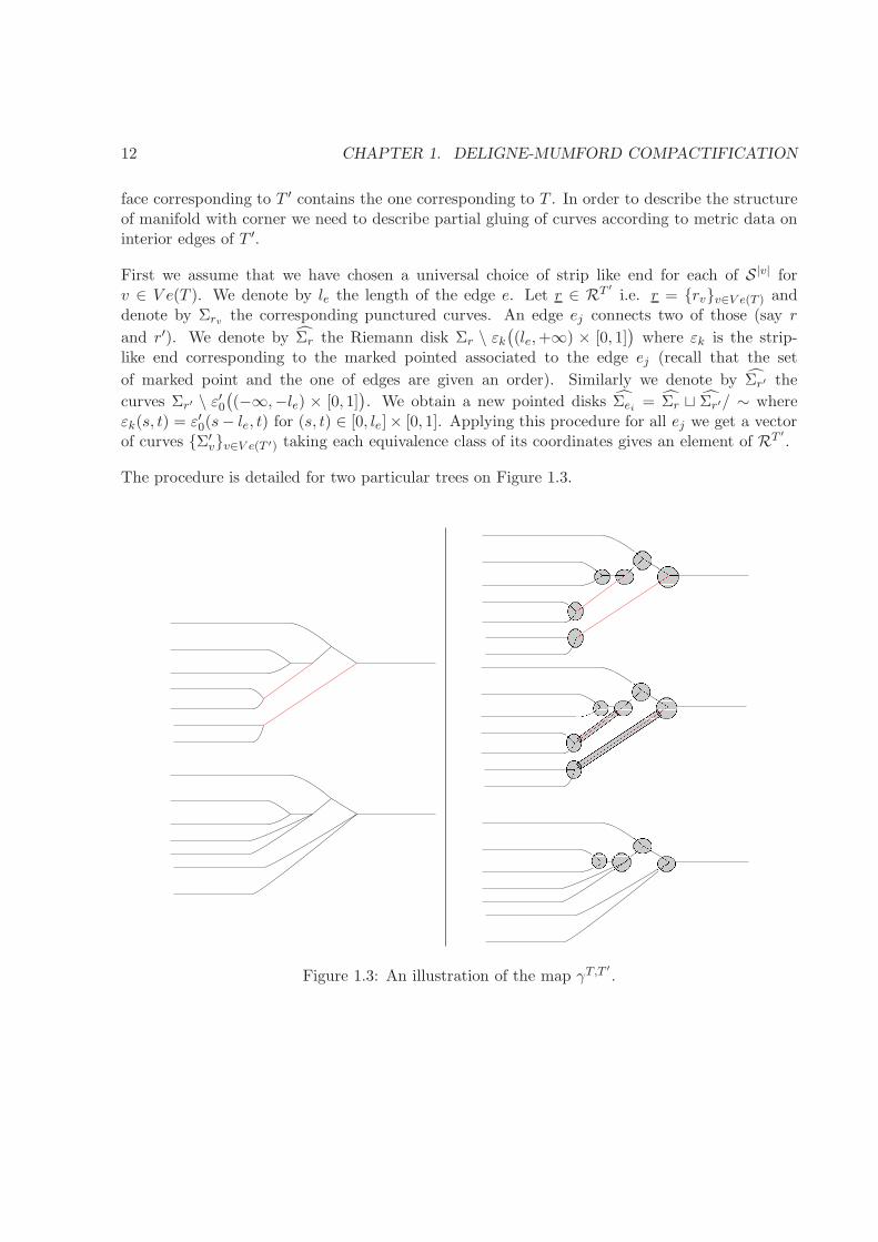
Recall that each faces of Kd is indexed by a tree T . Let T ′ be tree which is obtain from T becollapsing a set of interior edges e1 · · · ek. In terms of Stasheff’s polyhedron the boundary of the


face corresponding to T ′ contains the one corresponding to T . In order to describe the structureof manifold with corner we need to describe partial gluing of curves according to metric data oninterior edges of T ′.

First we assume that we have chosen a universal choice of strip like end for each of S |v| forv ∈ V e(T ). We denote by le the length of the edge e. Let r ∈ RT ′

i.e. r = rvv∈V e(T ) anddenote by Σrv the corresponding punctured curves. An edge ej connects two of those (say r

and r′). We denote by Σr the Riemann disk Σr \ εk((le,+∞) × [0, 1]

)where εk is the strip-

like end corresponding to the marked pointed associated to the edge ej (recall that the set

of marked point and the one of edges are given an order). Similarly we denote by Σr′ the

curves Σr′ \ ε′0

((−∞,−le) × [0, 1]

). We obtain a new pointed disks Σei = Σr ⊔ Σr′/ ∼ where

εk(s, t) = ε′0(s− le, t) for (s, t) ∈ [0, le]× [0, 1]. Applying this procedure for all ej we get a vectorof curves Σ′

vv∈V e(T ′) taking each equivalence class of its coordinates gives an element of RT ′

.

The procedure is detailed for two particular trees on Figure 1.3.

Figure 1.3: An illustration of the map γT,T′

.

1.5. CONSISTENT CHOICE OF STRIP-LIKE ENDS. 13

Thus this procedure defines a (smooth) map

γT,T′

: RT × (−1, 0)k → RT ′

(1.1)

where we use ρe = −e−πle as new gluing parameter. This allows us to define a topology on Rd+1

by setting maps to be continuous when pre-composed with the γT,Td .

Theorem 1.4.1. The Deligne-Mumford space Rd+1 is a manifold with corner where the boundarycharts are given by γT,Td where Td is the d+ 1 stable rooted tree with only one interior vertices.We extend γT,Td to RT × (−1, 0]k by

γT,Td(Σ, ρ1, . . . , 0, ρ2, 0, . . . , 0, ρi, 0, . . . , 0, ρi+1 . . . , 0, . . . , ρk) := γT,T′

(Σ, ρ1, . . . , ρk)

where T ′ is obtained from T by collapsing only edges with non zero gluing parameter.

This manifold with corner is diffeomorphic to the polyhedron Kd.

Before giving a proof of this we begin with an exercise.

Exercise 1.4.1. Show that the topology on Rd+1 does not depend on the choice of strip-likeends.

Proof. The proof decomposes as a sequence of exercises.

Exercise 1.4.2. 1. Show that the maps γT,T′

are smooth and prove that when ρ << 1 thed(γ(r,ρ) is invertible.

2. Deduce that for small enough parameters γT,T′

are open embeddings.

3. Show that with the induced topology Rd+1 is Hausdorff and compact.

4. * Find an embedding of Rd+1 into the convex realisation of Kd.

1.5 Consistent choice of strip-like ends.

Now given a universal of choice of strip-like ends for each of the Sd a curve Σr for r ∈ Rd in theimage of a gluing map γT,Td admits two sets of strip-like ends: the one given by the universal


choice on Sd and the second given by the universal choice on S |v| for all vertices v of T and thegluing map (1.1). We say that the universal choices of strip-like ends for each Rd is consistent

if for all d there is a neighbourhood U of ∂Rd in Rd on which on those sets of strip-like endscoincides.

Gluing parameters ρ for which γT,Td(RT , ρ) is inside U are said sufficiently small.

We now state the following theorem.

Theorem 1.5.1. Consistent choice of strip-like ends exists.

Proof. We proceed by induction. Assume that we have universal choices of strip-like ends for eachRd′+1 for d′ < d such that there exists neighbourhood Ud′+1 of ∂Rd′+1 satisfying the consistencycondition. We now want to build a universal choice of strip-like ends on Rd together with aneighbourhood Ud+1 satisfying the consistency condition.

For ǫ > 0 we denote by UTǫ the image of RT × [0, ǫ)|T |. We choose ǫ0 sufficiently small such that

• Each of the UTǫ0

are diffeomorphic images of RT × [0, ǫ0)|T |

• If T1 and T2 have no faces in common (of any codimension) then UT1ǫ0 ∩ UT2

ǫ0 = ∅.

• UT1ǫ0 ∩ UT2

ǫ0 = UT ′

ǫ0where T ′ is the tree which can collapse to both T1 and T2.

That such ε0 exists follows from Exercise 1.4.2.

Let r ∈ UT1ǫ0

∩ UT2ǫ0. T1 and T2 a priori determine two different sets of strip-like ends for Σr, we

will show that under our induction hypothesis those two sets coincides. First note that sinceUT1ǫ0

∩ UT2ǫ0

6= ∅ this implies that there is a tree T ′ which is in a face of both ∂T1 and ∂T2in other

word there are edges l11 . . . l1k1

and l21 . . . l2k2

of T ′ such that the collapse of lji gives Tj.

Let ρje for e interior edges of Tj and rv1 ∈ R|v| for v vertex of Tj such that r = γTj ,Td(rj, ρj).

For gluing parameter ρ for γT′,Td we denote by ρj the corresponding parameter for γT

′,Tj givenby the obvious projection. The remaining parameters are denoted ρj,c.

From the definition of the gluing maps γ it is clear that γT′,Td(r, ρ) = γTj ,Td(γT

′,Tj(r, ρj), ρj,c).And since we restricted the gluing parameters such that each gluing map are open embedding,it follows from the fact that r = γT1,Td(r1, ρ1) = γT2,Td(r2, ρ2) that there exist r and ρ such that

r = γT′,Td(r, ρ). Since γT

′,Tj (r, ρj) = (rj) our inductive hypothesis implies that all strip-like ends

1.6. LAGRANGIAN LABELS. 15

of component of Σrj are induced by the component of Σr. This implies that the strip-like endsinduced by Σr1 on Σr are the same as the one induced by Σr2 which are the one induced by Σr.

All in all, this implies that our hypothesis determines strip-like ends on ∪UTǫ0. It is now easy

to extend this choice of strip-like end on the whole Rd similarly to the construction of Exercise1.3.1.

From now on we assume that the associahedra Rd+1 are equipped with a consistent choice ofstrip-like ends.

1.6 Lagrangian labels.

A label for a stable (or semi-stable) tree by a discrete label set E is simply a continuous functionform R

2 \ T to E (i.e. to each connected component of R2 \ T we assign an element of E).

Exercise 1.6.1. Show that if T belongs to a faces of T ′ then any label for T extends naturallyto a label of T ′.

Using the correspondence between Kd and Rd+1 labels has the following meaning. To any interiorvertex v of T corresponds a pointed disks Dv. The connected component of ∂D correspond toquadrant of v (a “local” connected component of R2 \ T ). Hence a label assign a label to eachconnected component of Dv. The condition that the labels are the same on global connectedcomponent implies that the assignment is consistent with the gluing operation γT,T

′

(similarlyto Exercise 1.6.1).

In the next chapter, the label set will be the set of Lagrangian sub-manifolds of a symplecticmanifold and we will use them as boundary condition for holomorphic maps.


Chapter 2

Naive tentative to define Fukaya

category.

This chapter serves as a second introduction to the class. We want, using very elementary con-siderations, to emphasise why consistent choices of perturbation data are necessary to have a welldefined Fukaya category. We allows ourselves to be sloppy and won’t highlight any of the tech-nical details we will address in the subsequent chapters. The precise statement on transversalityand compactness will appears later.

At the end of the chapter there is an exercise which aims to emphasise the differences betweenhigher order operations in the Donaldson category and higher order operations in the Fukayacategory.

From now on we assume that (M,dθ) is the completion of a Liouville manifolds and that La-grangian labels are taken in Lag(M) the set of exact Lagrangians which are conical outside acompact set. We also pick a compatible almost complex structure J on M .

2.1 Holomorphic curves.

Let L be Lagrangian labels for Rd+1 and let ai ∈ Li ⋔ Li+1 (with the convention that Ld+1 isL0). Given r ∈ Rd+1, we decompose ∂(Σr) = ⊔d

i=1 according to its connected component orderedcounter-clockwise. We denote by Mr

L(a0; a1, . . . , ad)) the set of maps u : Σr →M such that

17

18 CHAPTER 2. NAIVE TENTATIVE TO DEFINE FUKAYA CATEGORY.

• du jr = J du.

• u(∂i) ⊂ Li.

• lims→−∞(u(ε0(s, t)) = a0.

• lims→∞(u(εi(s, t)) = ai.

We denote by ML(a0; a1, . . . , ad) := ∪r∈Rd+1MrL(a0; a1, . . . , ad). By definition the Ck

loc-topology

on M is induced by the Ck-topology on Mr and the requirement that the projection to Rd+1. Itfollows from Gromov’s compactness that a 1-parameter family of elements ut ofML(a0; a1, . . . , ad)can be compactified into manifolds with boundary where the boundary points are of two types:

• Stable-breaking: the domain rt of ut converges to r0 ∈ ∂Rd+1 and the maps ut converges to apair of holomorphic curves inMLT1

(a0; a1, . . . , ai−1, a′i, ai+j , . . . ad)×MLT1

(a′i; ai+1, . . . , ai+j)

• Semi-stable breaking: the domain rt converges to r0 ∈ Rd and the maps ut converges to apair of maps in either ML(a0; a1, . . . , a

′i, . . . , ad) ×MZ

Li,Li+1(a′i, ai) or in MZ

Ld,L0(a0, a

′0) ×

ML(a′0; a1, . . . , ad).

2.2 Gromov compactness in action.

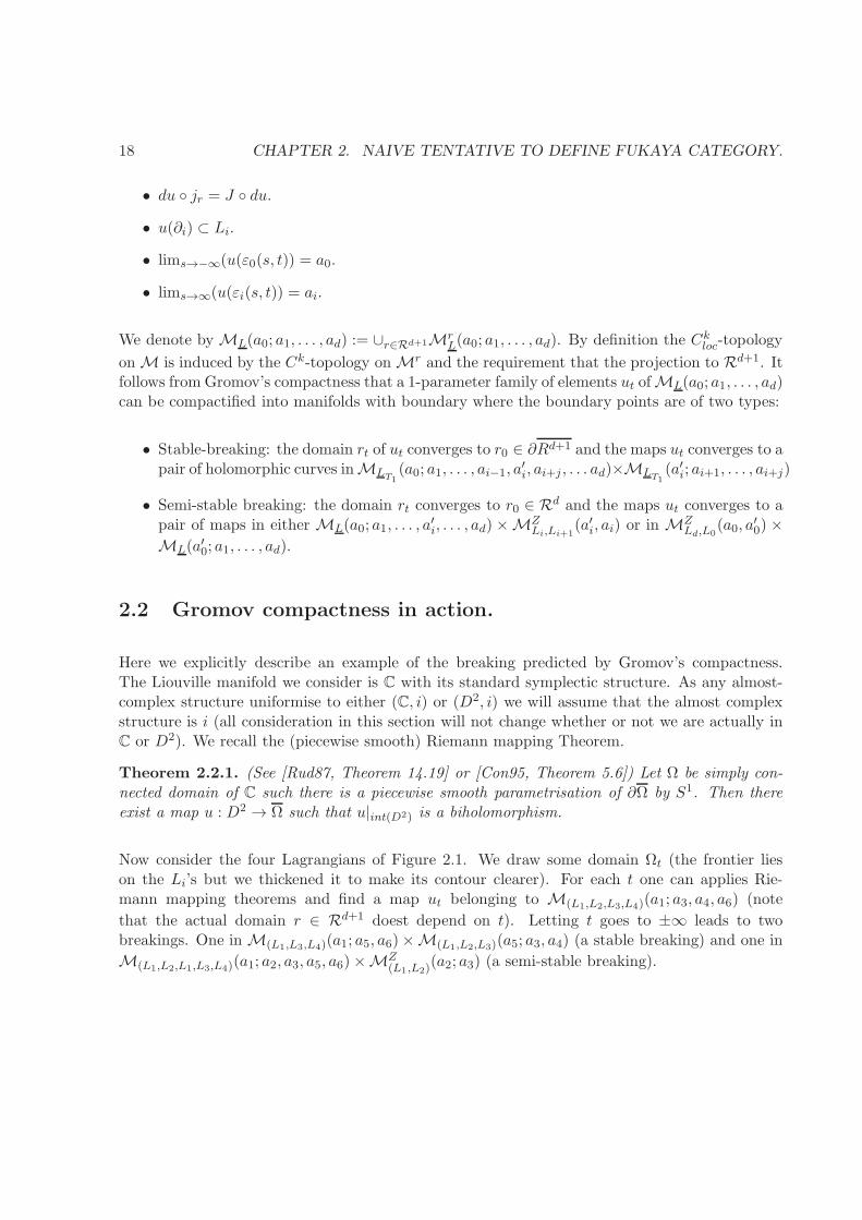
Here we explicitly describe an example of the breaking predicted by Gromov’s compactness.The Liouville manifold we consider is C with its standard symplectic structure. As any almost-complex structure uniformise to either (C, i) or (D2, i) we will assume that the almost complexstructure is i (all consideration in this section will not change whether or not we are actually inC or D2). We recall the (piecewise smooth) Riemann mapping Theorem.

Theorem 2.2.1. (See [Rud87, Theorem 14.19] or [Con95, Theorem 5.6]) Let Ω be simply con-nected domain of C such there is a piecewise smooth parametrisation of ∂Ω by S1. Then thereexist a map u : D2 → Ω such that u|int(D2) is a biholomorphism.

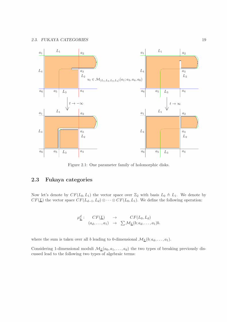
Now consider the four Lagrangians of Figure 2.1. We draw some domain Ωt (the frontier lieson the Li’s but we thickened it to make its contour clearer). For each t one can applies Rie-mann mapping theorems and find a map ut belonging to M(L1,L2,L3,L4)(a1; a3, a4, a6) (note

that the actual domain r ∈ Rd+1 doest depend on t). Letting t goes to ±∞ leads to twobreakings. One in M(L1,L3,L4)(a1; a5, a6)×M(L1,L2,L3)(a5; a3, a4) (a stable breaking) and one in

M(L1,L2,L1,L3,L4)(a1; a2, a3, a5, a6)×MZ(L1,L2)

(a2; a3) (a semi-stable breaking).

2.3. FUKAYA CATEGORIES 19

ut ∈ M(L1,L2,L3,L4)(a1; a3, a4, a6)

L1

L2

L3

L4

a1 a2

a3

a4a5a6

L1

L2

L3

L4

a1 a2

a3

a4a5a6

L1

L2

L3

L4

a1 a2

a3

a4a5a6

L1

L2

L3

L4

a1 a2

a3

a4a5a6

t→ −∞ t→ ∞

Figure 2.1: One parameter family of holomorphic disks.

2.3 Fukaya categories

Now let’s denote by CF (L0, L1) the vector space over Z2 with basis L0 ⋔ L1. We denote byCF (L) the vector space CF (Ld−1, Ld)⊗ · · · ⊗ CF (L0, L1). We define the following operation:

µdL : CF (L) → CF (L0, Ld)

(ad, . . . , a1) →∑

ML(b; ad, . . . , a1)b.

where the sum is taken over all b leading to 0-dimensional ML(b; ad, . . . , a1).

Considering 1-dimensional moduli ML(a0, a1, . . . , ad) the two types of breaking previously dis-cussed lead to the following two types of algebraic terms:


• Stable:

µd1LT1(ad, . . . , µ

d2LT2

(ai+j, . . . , ai+1), ai−1, . . . , a1)

for d1, d2 > 1 such that d1 + d2 = d+ 1.

• Semi-stable:

(µ1 µd)(ad, . . . , a1).

As an illustration the two breaking of Figure 2.1 correspond to: µ2(a6, µ2(a4, a3)) and µ

3(a6, a4, µ1(a3))

respectively.

We assume that transversality (i.e. ML are manifolds) and gluing (any broken configurationsis at the boundary of some 1-dimensional moduli space) holds. Since boundary of compact 1-dimensional manifolds has even cardinality, we get that those terms add up to 0 which impliesthat the operations µd satisfies the A∞ Equation (1).

Following this one wish to define an A∞-category Fuk(M) in the following way:

• The objects Ob(Fuk(M)) is the set of exact Lagrangian sub-manifolds of (M,ω).

• The morphisms spaces are the Lagrangian Floer intersection complex (CF (L0, L1), µ1L0,L1

).

• Composition of morphisms is given by µ2L0,L1,L2: CF (L1, L2)⊗CF (L0, L1) → CF (L0, L2).

• Higher order compositions are given by the operation µL.

On the homological level this category should recover the Donaldson category where morphismsspaces are HF (L0, L1) := H(CF (L0, L1), µ

1L0,L1

) and compositions are given by the map induced

by µ2L0,L1,L2. Since Floer homology is invariant under Hamiltonian deformation there are well

defined endomorphisms spaces setting HF (L,L) := HF (L, φH(L)) for a generic small Hamilto-nian. However in the case of Fukaya categories things are different since the actual complex dodepend on φH .

This leads to serious problems as we need to consider perturbations of pair of Lagrangian sothat every time this given pair of Lagrangian is involved we actually see this very perturbation.Falling to do so would imply that the applications defined by Equation (1) would not have theappropriate domain or codomain. The same trouble arises when we want to define the higherorder operation in the non-transverse case and again perturbation are needed and consistencybetween those perturbation is required to have a well define theory. In order to illustrate theseproblems we illustrate this on some very simple examples.


L1

L0

L1

L0

φH(L0)

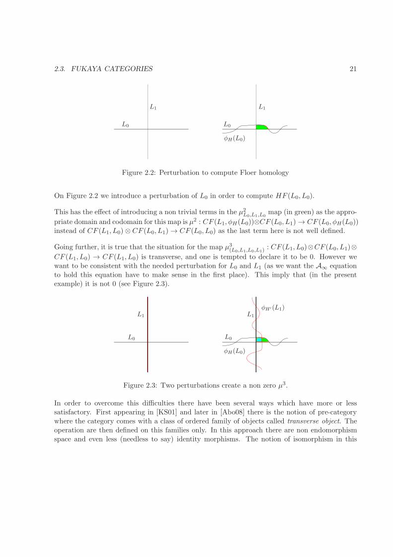
Figure 2.2: Perturbation to compute Floer homology

On Figure 2.2 we introduce a perturbation of L0 in order to compute HF (L0, L0).

This has the effect of introducing a non trivial terms in the µ2L0,L1,L0map (in green) as the appro-

priate domain and codomain for this map is µ2 : CF (L1, φH(L0))⊗CF (L0, L1) → CF (L0, φH(L0))instead of CF (L1, L0)⊗ CF (L0, L1) → CF (L0, L0) as the last term here is not well defined.

Going further, it is true that the situation for the map µ3(L0,L1,L0,L1): CF (L1, L0)⊗CF (L0, L1)⊗

CF (L1, L0) → CF (L1, L0) is transverse, and one is tempted to declare it to be 0. However wewant to be consistent with the needed perturbation for L0 and L1 (as we want the A∞ equationto hold this equation have to make sense in the first place). This imply that (in the presentexample) it is not 0 (see Figure 2.3).

L0

L1 L1

L0

φH(L0)

φH′ (L1)

Figure 2.3: Two perturbations create a non zero µ3.

In order to overcome this difficulties there have been several ways which have more or lesssatisfactory. First appearing in [KS01] and later in [Abo08] there is the notion of pre-categorywhere the category comes with a class of ordered family of objects called transverse object. Theoperation are then defined on this families only. In this approach there are non endomorphismspace and even less (needless to say) identity morphisms. The notion of isomorphism in this


category is thus subtle and the price we pay of not developing a more satisfactory theory is thatwe end up with an object not so easy to manipulate.

The other approach is to package the needed perturbations in a consistent way so that thecategory we define depends on this family of consistent perturbations. This have been mostsuccessfully done in the book of Seidel [Sei08] and we will describe this approach in this course,the next chapter is dedicated to the proof that such consistent choice of data and perturbationexists. Once we have a well define category we need to prove that the quasi-equivalence class ofthe category does not depends on those. It turns out that this is an easy tasks once we play withlots of algebraic non-sense as we will see in Chapter 5. The price we pay with this approach isthat the theory is not so computable any more.

To conciliate the two approaches: having something more computable on one side and an actualcategory on the other we rely on some method to find a finite set of generator of our category andthen on those generators we define the notion of directed category where endomorphism spaceare trivial (isomorphic to the coefficient ring) and consider that this new category still retainsa lot of information of the original category. This approach is again described in the third partof Seidel’s book. In the present course we will focus on some methods to find generators of theFukaya category developed by Abouzaid in [Abo10] and implement it for the case of surface inChapter 6.

Before we go into the details of the construction we still ask for a little longer the reader to havefaith in the well definiteness of this category and give some small intuitive exercise so that hefamiliarises himself with those operation and see the differences between these and the one whichappeared earlier in the Donaldson category.

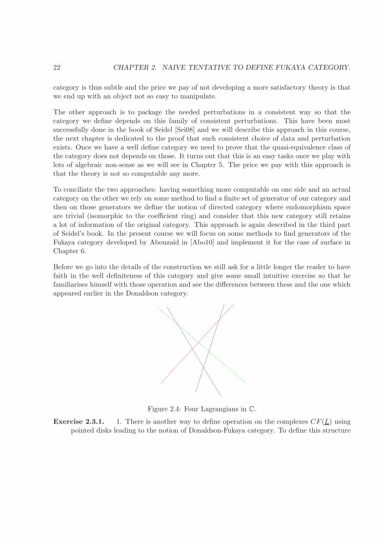
Figure 2.4: Four Lagrangians in C.

Exercise 2.3.1. 1. There is another way to define operation on the complexes CF (L) usingpointed disks leading to the notion of Donaldson-Fukaya category. To define this structure


we consider similar moduli space with the difference that we fix the conformal structure onthe surface. More precisely for a generic r ∈ Rd+1 we define:

mdL : CF (L) → CF (L0, Ld)

(ad, . . . , a1) →∑

MrL(b; ad, . . . , a1)b.

Convince yourself that this lead to a well defined operation md on the complexes whichinduces application on homology groups.

2. Find an heuristic argument which prove that all maps md are characterised in homologyby m2 (which is actually equal to µ2).

3. Compute µ1, µ2, µ3 and m3 on the non-compact Lagrangians shown on Figure 2.4.

4. Verify theA∞-relation for the operation µ and the Frobenius type relation found on question2 for the operation m.


Chapter 3

Perturbed Floer equation and

perturbation data.

3.1 Floer data.

To achieve transversality of intersection for any pair of intersection we make the following defi-nition.

Definition 3.1.1. Let L0 and L1 be a pair of Lagrangian sub-manifolds of (M,ω). A Floerdatum for (L0, L1) is

• A time dependent Hamiltonian function H :M × [0, 1] → R such that φH(L0) ⋔ L1.

• A time dependant almost complex structure Jt t ∈ [0, 1] compatible with ω.

Given a pair of Lagrangian sub-manifolds, a Floer datum gives a Floer complex:

CF (L0, L1;H,J) := Z2(φH(L0) ⋔ L1).

Note that there is a bijection between φH(L0) ⋔ L1 and trajectories γ : [0, 1] of XH such thatγ(0) ∈ L0 and γ(1) ∈ L1. For a ∈ φH(L0) ⋔ L1 we denote by γa the corresponding trajectory ofXH .

25

26 CHAPTER 3. PERTURBED FLOER EQUATION AND PERTURBATION DATA.

Under transversality assumptions, the Floer complex is equipped with a differential µ1L0,L1;H,J(b) =∑< a, b > a where < a, b > is defined as a count of maps u : Z →M such that:

u(·, 0) ∈ L0

u(·, 1) ∈ L1

lims→−∞u(s, t) = γa(t)

lims→∞u(s, t) = γb(t)

∂su+ Jt(u)(∂tu−XHt(u)

)= 0. (3.1)

From now on we assume that any pair of Lagrangian comes with a given Floer datum such thatsolution to (3.1) are transversely cut-out and we drop both J and H from the notation.

In order to justify the following equation with respect to the consideration of previous chapterlet’s consider a curve v : R× [0, 1] →M which satisfies the following:

v(·, 0) ∈ φH(L0)

v(·, 1) ∈ L1

lims→−∞v(s, t) = a

lims→∞v(s, t) = b

∂sv + J(v)(∂tv −XHt(v)

)= 0.

We define u(s, t) = (φH1−t)−1(v(s, t) then

• u(·, 0) ∈ (φH)−1(φH(L0) = L0.

• u(·, 1) ∈ L1.

• lims→−∞ u(s, t) = (φH1−t)−1(a) = γa(t)

• lims→∞ u(s, t) = (φH1−t)−1(b) = γb(t).

To check which equation u satisfies we compute:

∂u

∂s= dφH1−t0

(∂v

∂s)

and

3.2. PERTURBATION DATA 27

∂u

∂t= dφH1−t0

(∂v

∂s+XH

1−t((φH1−t)

−1(v)).

If we define Jt by (φH1−t)−1J then u satisfies

∂u

∂s+ Jt(

∂u

∂t−XH

t = 0.

Hence the perturbed Floer complex for L0 and L1 is the unperturbed on for φH(L0) and L1.

3.2 Perturbation data

Let Σ ∈ Rd together with a Lagrangian label L for Σ. In order to interpolate between thedifferent Floer data associated to the marked point of Σ we introduce the notion of perturbationdatum.

Definition 3.2.1. A perturbation datum for (Σ, L) is a pair (K,J) where

• K ∈ Ω1(Σ, C∞0 (M)) such that

1. For all ξ T∂iΣr K(ξ)|Li= 0.

2. ε∗yiK = Hyidt.

• J ∈ C∞(Σ,J ) such that J |εyi(s,t(s, t) = JLi−1,Li(t).

Given such a perturbation datum we have an associated perturbed Cauchy-Riemann equationfor maps u : Σ →M such that u(∂(Σ)) ∈ L which is

du(z)(ζ) + J(z, u) du(z) jΣ(ζ) = XK(ζ) + J(z, u) XK(jΣζ). (3.2)

u(∂iΣr) ⊂ Li)

lims→±∞

u(εi(s, t)) = γi(t).

For short we sometime write the first equation as du0,1 = (XK)0,1 or (du−Xk)0,1 = 0.

Exercise 3.2.1. 1. If the perturbation datum on the Z is given by J(s, t) = J(t) and K =H(t)dt then prove that Equation (3.2) reduces to Equation (3.1).


2. Let H0 and H1 be two time-dependent Hamiltonian functions let K = Hsdt be a part of aperturbation datum for Z between the two Floer data associated to H0 and H1. Assumingtransversality, gluing and compactness show that the counts of solution to Equation (3.2)induces the comparison map from CF (L0, L1,H0) to CF (L0, L1,H1).

3.3 Consistent choices of perturbation data.

Suppose that for all d′ ≤ d we have chosen perturbation data (Kr, Jr) for all r ∈ Rd′+1

Take a curve r in the image of the gluing map where parameter are sufficiently small in Rd+1. Asthe gluing parameter is sufficiently small, the strip-like end coincide with the one coming fromthe curves rv for v ∈ V e(T ) prior to gluing and thus the data given by (Kv, Jv) are compatiblewith the strip like ends and thus are perturbation data for r. This implies that r has two set ofperturbation data. We need a definition of consistency for these choice of perturbation, which willallows us to say that Gromov breaking of solution of Equation (3.2) converge to broken solutionfor the boundary perturbation data.

Note that r comes with a thin-thick decomposition where the thin part is made of the image ofthe strip-like ends of the rv after the gluing (this is made of the strip-like ends of r plus someinterior “rectangle”). Note that from the construction of the gluing map the union of the thickparts of the rv’s is the thick part of r. The appropriate notion of consistency is the following.We say that choices of perturbation data are consistent if

• The two previous perturbation data agrees on the thin part of r.

• If rn → rv for n → ∞ (i.e. rn = γT,Td(ρnv , rnv ) with ρnv → 0 and rnv → rv) then

the perturbation data on rn converges to the family of perturbation data Kv, Jv thisconvergence make sense if the first condition is satisfied as it ensure that we need only toconsider convergence on the thick part.

Note in particular that if the data do agree on the whole of r then the data are consistent, aschoices of perturbation data are contractible (because C∞

0 (M) and J (ω) are) we can apply thesame proof as of Theorem 1.5.1 to prove

Proposition 3.3.1. Consistent choices of perturbation data exists.

Remark 3.3.2. The reason for having a weaker notion of consistent perturbation data will appearin Chapter 5 for transversality consideration, where will modify some consistent choice intogeneric one to guarantee that solutions to Equation (3.2) form a manifold.

3.4. LINEARISATION OF EQUATION (3.2) 29

3.4 Linearisation of Equation (3.2)

We now turns our attention to the linearisation of Equation (3.2) and try to describe it as astandard Cauchy-Riemann operator (i.e. the 0, 1-part of a covariant derivative).

We recall the definition of such operators.

Definition 3.4.1. Let E → Σr be a symplectic vector bundle with compatible complex multipli-cation J . Let F be Lagrangian sub-bundle of E on ∂Σr (i.e. for q ∈ ∂Σr Fq is a Lagrangiansubspace of Eq. We denote by Γ(E,F ) the space of section s of E such that sq ∈ Fq for allq ∈ ∂Σr. A real Cauchy-Riemann operator D on E is a linear map:

D : Γ(E,F ) → Ω0,1Σr

(E)

satisfying:

∀f ∈ C∞(Σr,R) D(fs) = fD(s) + ∂f ⊗ s.

Remark 3.4.2. One way to construct such a operator is to take any connexion ∇ and take its 0, 1part ∇0,1. All real Cauchy-Riemann operator are actually of this forms, for details see [MS04,Appendix C].

The goal of this section is to show that the linearisation of Equation (3.2) is a real Cauchy-Riemann operator. We first describe what is this linearisation process. Let Br the space ofsmooth 1 maps from Σr to M with the boundary condition given by the Lagrangian label L. Itsformal tangent space at u is TuBr = V Γ(u∗TM)|∀q ∈ ∂iΣrVq ∈ Tu(q)Li (note that those aresections of a symplectic vector bundle with prescribed Lagrangian condition on the boundary).Let E be the vector bundle over Br whose fibre over u is Ω0,1

Σr(u∗TM) the space of 1-forms of

type 0, 1 over Σr with values in TM . Equation (3.2) defines a section of ν of this bundle by

ν(u)q(ξ) = duq(ξ) + J(q)(duq(jrξ)

)− X

K(ξ)q − J(q)

(X

K(jrξ)q

). Let πu : T(u,0)E → Eu be the

projection parallel to TuBr where Br is the 0-section. Let u0 be a solution of Equation (3.2), thelinearisation of Equation (3.2) at u0 is

Du0 : Tu0B → Ω0,1Σr

(u∗0TM)

defined by Du0(V ) = πu0dν(V ).

Proposition 3.4.3. The operator Du0 is a real Cauchy-Riemann operator.

1the actual regularity W1,p necessary to have a Fredholm operator will be detailed in the next section


Proof. It suffices to show that Du0(fV ) = fDu0(V ) + ∂(f)V for all f ∈ C∞(Σr).

Chapter 4

Grading.

4.1 Maslov index.

Let (V, ωV ) be a symplectic vector space of dimension n on which we choose a compatible almoststructure JV . We denote by Gr(V, ωV ) the Grassmanian of Lagrangian subspace of V . If onechoose a reference Lagrangian subspace λ0, it is identified as the orbit of an U(n) action (theaction of U(n) as symplectic transformation is given by JV ). It is thus an homogeneous spaceU(n)/O(n). This identification lead to a map αV := det2 : Gr(V, ωV ) → S1 which induce anatural map

µ : H1(Gr(V, ωV ) → Z = H1(S1).

In the next section we will need another description of the map αV . Fix an identification η2V :ΛtopC

⊗ ΛtopC

≃ C and note that for a basis (v1, . . . , vn) of an element L ∈ Gr(V, ωV ) we have thatη2V (v1 ∧ . . . ∧ vn ⊗ v1 ∧ . . . ∧ vn) 6= 0 (since L is Lagrangian we have that L⊕ JL = V ).

We have the following proposition:

Proposition 4.1.1. For another basis (w1, . . . , wn) of L we have that η2V (w1 ∧ . . . ∧ wn ⊗ w1 ∧. . . ∧ wn) = (detP )2η2V (v1 ∧ . . . ∧ vn ⊗ v1 ∧ . . . ∧ vn) where P is the change of basis matrix.

Proof. Simply note that P ∈ Gln(R) extends to a transformation P of V via the inclusionGln(R) ⊂ GLn(C) mapping vi to wi. The results follows from the definition of Λtop

C.

This implies that the valueη2V (v1∧...∧vn⊗v1∧...∧vn)

||η2V(v1∧...∧vn⊗v1∧...∧vn)||

∈ S1 only depends on L. This is related to

31

32 CHAPTER 4. GRADING.

the function αV noticing that choosing a referenced subspace λ0 and a basis for λ0 gives anidentification η2V just mapping v1 ∧ . . . ∧ vn ⊗ v1 ∧ . . . ∧ vn to 1 ∈ C. An easy verification showsthat the to maps to S1 corresponds.

The maslov index of a loop λ in Gr(V, ωV ) is µ([λ]) ∈ Z.

Given a path λ(r)r∈(−ε,+ε) in Gr(V, ωV ) we choose applications φr such that φs = Id andφr(λ(0)) = λ(r).

Proposition 4.1.2. Let λ1 ∈ Gr(V, ωV ) the following quadratic forms on Lλ(0),Λ1= λ(0) ∩ λ1is

independent of the choice of the map φr

qλ,λ1(v) := −d

dr|r=0ωV (φr(v), v) = −ωV (

d

dr|r=0φr(v), v) (4.1)

Proof. Let ψr be a map with the same properties as φr. Then there are linear maps fr : V → Vsuch that f0 = Id and φr fr = ψr (note that this implies that fr preserves λ(0)).

We get that

d

dr|r=0ψr(v) =

d

dr|r=0φr fr(v)

=d

dr|r=0φr(f0(v)) + φ0(

d

dr|r=0fr(v)) =

d

dr|r=0φr(v) +

d

dr|r=0fr(v)

Since fr preserves λ0 we get that fr(v) ∈ λ0 ∀r and thus that ddr|r=0fr(v) ∈ λ0. Since λ0 is

Lagrangian we get that wV (ddr|r=0fr(v), v) = 0 and the result follows.

Definition 4.1.3. Given a path λ : [0, 1] → Gr(V, ωV ) we define the crossing formof λ ats ∈ (0, 1) to be the form on λ(s) ∩ λ1 defined by

qλ,λ1(s) := qλs,λ1

where λs is defined on some (−εs, εs) by λs(r) = λ(s+ r).

For a generic loop, the intersection of λ(s) with λ1 is not 0 only for a finite number of time s,therefore the following proposition make sense.

4.1. MASLOV INDEX. 33

Proposition 4.1.4. For a generic loop λ : [0, 1] → Gr(V, ωV ) such that λ(0) = λ(1) ⋔ λ1 wehave

µ(λ) =∑

0<s<1

ind(qλ,λ1(s)). (4.2)

We will need a small variation of this concept for some special paths in Gr(V, ωV ). We denote byP−(Gr(V, ωV )) the space of paths λ : [0, 1] → Gr(V, ωV ) such that λ(0) ⋔ λ(1) and qλ,λ(1)(1) isnegative definite. Similarly to Proposition 4.1.4 we define for a generic path in P−(Gr(V, ωV )):

ι(λ) =∑

0<s<1

ind(qλ,λ(1)(s) (4.3)

We denote by Gr#(V, ωV ) the pull-back of the cover exp(i·) : R → S1 by αV (it is one realisationof the universal cover of Gr(V, ωV ). And we denote by π the canonical projection to Gr(V, ωV ).An element (L,α#) in Gr#(V, ωV ) is called a graded Lagrangian subspace.

Let (L1, α#1 ) and (L2, α

#2 ) be two grade Lagrangian subspace such that L1 ⋔ L2. There exist up

to homotopy a unique path λ# from (L1, α#1 ) to (L2, α

#2 ) such that π λ# is in P−(Gr(V, ωV )).

We define the index of the pair to be

ι((L1, α#1 ), (L2, α

#2 )) = ι(π λ#) (4.4)

We encourage the reader to do the following exercise so that he familiarise himself with theMaslov index of path.

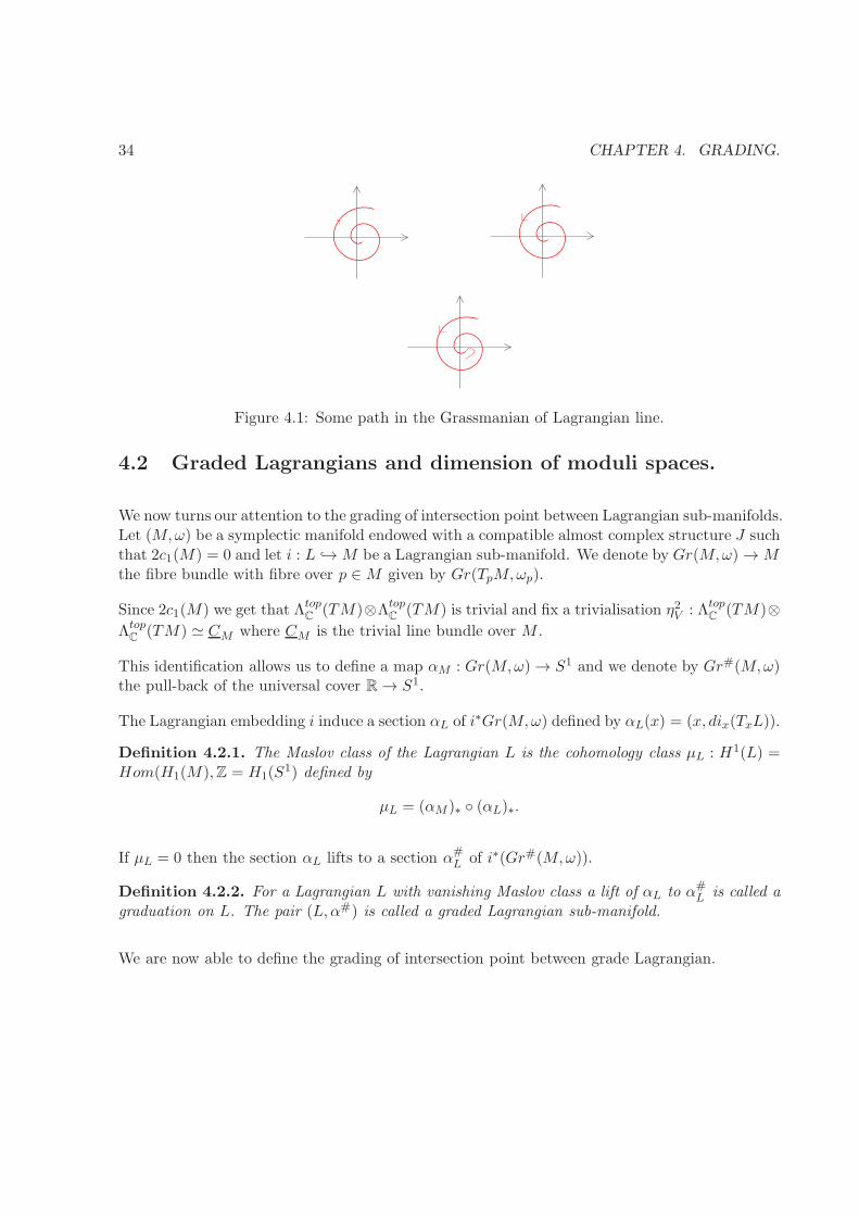
Exercise 4.1.1. 1. Each of the red curves of Figure 4.1 gives a path in Gr(C, ω0) by taking theargument of the curves (pay attention that in Gr(V ) we consider unoriented Lagrangian).For each of them tells if the given path is in P− and if yes compute its index.

2. Let L#1 = ((t, 0)|t ∈ R, 6π) and L#

2 = ((t, t)|t ∈ R, 3π/4) be two elements ofGr#(C, ω0).

Compute ι(L#1 , L

#2 ) and ι(L

#2 , L

#1 ).

3. Show that in general ι(L#1 , L

#2 ) = n− ι(L#

2 , L#1 ) where 2n is the dimension of V .


Figure 4.1: Some path in the Grassmanian of Lagrangian line.

4.2 Graded Lagrangians and dimension of moduli spaces.

We now turns our attention to the grading of intersection point between Lagrangian sub-manifolds.Let (M,ω) be a symplectic manifold endowed with a compatible almost complex structure J suchthat 2c1(M) = 0 and let i : L →M be a Lagrangian sub-manifold. We denote by Gr(M,ω) →Mthe fibre bundle with fibre over p ∈M given by Gr(TpM,ωp).

Since 2c1(M) we get that ΛtopC

(TM)⊗ΛtopC

(TM) is trivial and fix a trivialisation η2V : ΛtopC

(TM)⊗

ΛtopC

(TM) ≃ CM where CM is the trivial line bundle over M .

This identification allows us to define a map αM : Gr(M,ω) → S1 and we denote by Gr#(M,ω)the pull-back of the universal cover R → S1.

The Lagrangian embedding i induce a section αL of i∗Gr(M,ω) defined by αL(x) = (x, dix(TxL)).

Definition 4.2.1. The Maslov class of the Lagrangian L is the cohomology class µL : H1(L) =Hom(H1(M),Z = H1(S

1) defined by

µL = (αM )∗ (αL)∗.

If µL = 0 then the section αL lifts to a section α#L of i∗(Gr#(M,ω)).

Definition 4.2.2. For a Lagrangian L with vanishing Maslov class a lift of αL to α#L is called a

graduation on L. The pair (L,α#) is called a graded Lagrangian sub-manifold.

We are now able to define the grading of intersection point between grade Lagrangian.

4.3. INDEX THEOREM FOR CAUCHY-RIEMANN OPERATORS ON THE DISK. 35

Definition 4.2.3. Let (L1, α#1 ) and (L2, α

#2 ) be two graded Lagrangian sub-manifold such that

L1 ⋔ L2. For p ∈ L1 ∩ L2 we define the degree of p by

ι(p) = ι((α#1 (p), α

#2 (p)) (4.5)

Note that the preceding definition make sense because since p ∈ L1 ∩ L2 then both α#1 (p) and

α#2 (p) belongs to Gr

#(TpM,ωp).

Let φH a symplectomorphism. Since symplectomorphisms preserves Lagrangians, d(φH)p inducesa map from Gr(TpM,ωp) to Gr(TφH (p)M,ωφH (p)) which extends to a map from Gr#(TpM,ωp)

to Gr#(TφH (p)M,ωφH(p)). This implies that a graded Lagrangian (L,α#L ) is naturally mapped to

a graded Lagrangian (φH(L), (φH )∗α#L ). If φH is Hamiltonian then a Hamiltonian chord y from

L1 to L2 corresponds to an intersection point between φH(L1) and L2. If (L1, α#1 ) and (L2, α

#2 )

are graded, we define the degree of this chord to be ι(y) = ι(p) where p is the correspondingintersection point.

We can now state the result which compute the expected dimension of Mr(y0; y1, . . . , yd).

Theorem 4.2.4. Let u ∈ Mr(y0; y1, . . . , yd) then

ind(Du) = ι(y0)−d∑

j=1

ι(yj).

The next section is devoted to the proof Theorem 4.2.4.

4.3 Index theorem for Cauchy-Riemann operators on the disk.

We will now explain the index theory for Cauchy-Riemann operators over pointed disks. Westart by the compact example.

Let (E,ωE) → D2 be a symplectic vector bundle of dimension n and let F ⊂ i∗E be a Lagrangiansub-bundle (with i : S1 → D2 the boundary inclusion). For p > 2 we denote by W 1,p(E,F ) thespace of W 1,p section of E with value in F on S1. Up to homotopy there is a unique symplectictrivialisation of E under which F correspond to a loop λ ∈ Gr(Cn, ω0).

The space W 1,p(E;F ) is the appropriate domain for real Cauchy-Riemann operators on Γ(E;F ).So let

D :W 1,p(E;F ) → Lp(E)


be a real Cauchy-Riemann operator (i.e. satisfying D(f · s) = f ·Ds + ∂f · s for all real valuedfunction).

The following is a relative version of Riemann-Roch Theorem (see [GH78, Chapter 2] for theclosed version):

Theorem 4.3.1. [MS04, Appendix C] The operator D is Fredholm and its index is

ind(D) = n+ µ(γ) (4.6)

We now turn our attention to the case of disks with marked point on their boundary. Fix r ∈ Rd+1

and let E → Σr be a symplectic vector bundle with compatible almost complex structure J . LetF be a Lagrangian sub-bundle of the bundle on the boundary, and we denote by Fi its restrictionto ∂iΣr. We denote again by W 1,p(E;F ) the space of W 1,p sections of E with boundary value inF and consider a real Cauchy-Riemann operator

Dr :W1,p(E;F ) → Lp(E).

given by the 0, 1-part of a connection ∇.

Definition 4.3.2. A set of limiting data is given by:

• A symplectic vector bundle (E′, ωE′) over [0, 1].

• Some Lagrangian subspace Λi of (E′i, ωi) for i = 0, 1.

• A compatible almost complex structure on E′.

• A symplectic connection ∇′ on E.

For i = 0, . . . d the operator Dr is compatible with a set of limiting data (Ei, ωi,Λi,0,Λi,1, Ji,∇i)if (assuming the end is outgoing)

• There exist an identification ψ : ε∗iE ≃ π∗Ei (where π : Z → [0, 1] is the canonicalprojection).

• lims→∞ ψj,t(Fj,t) = Λi,j for j = 0, 1.

• The difference ωE − ωi|s=s0 , J − Ji|s=s0 and ∇ − ∇i converges exponentially to 0 in theC1-norms.

4.3. INDEX THEOREM FOR CAUCHY-RIEMANN OPERATORS ON THE DISK. 37

If Dr has compatible limiting data for i = 1, · · · , d we say that Dr is admissible if ∀i the paralleltransport Λi,0 of Λi,0 by ∇i along [0, 1] is transverse to Λi,1.

Exercise 4.3.1. Show that the Cauchy-Riemann operator of Section 3.4 is admissible.

Note that since all boundary condition are over open interval, one can lift all of those toGr#(E|∂Σr

) and that the convergence induces lifts Λ#i,j which by parallel transport induces lifts

Λ#i,0 and Λ#

i,1

Theorem 4.3.3. If Dr is admissible then it is Fredholm, its index is

i(Λ#j,0,Λ

#0,1)−

d∑

j=1

i(Λ#j,0,Λ

#j,1) (4.7)

for any lift of the Lagrangian boundary conditions Fi.

Theorem 4.2.4 is then an immediate consequence of Theorem 4.3.3.

We will prove Theorem 4.3.3 in three step. First we proof a gluing formula for CR operator.Then we proof the formula for a particular boundary condition over H and finally we prove thegeneral formula.

4.3.1 Gluing operators

4.3.2 Operators over H

4.3.3 Proof of the index formula


Chapter 5

Fukaya categories.

We are now ready to wrap everything together and define the Fukaya category of an exactsymplectic manifold.

5.1 Definition of Fuk(M,ω).

We are now ready to give the definition of the Fukaya category of an exact symplectic manifoldsM . We assume that we have chosen a consistent choice of strip-like ends for all Stasheff polyhedraRd+1, some transverse Floer data for all pairs of Lagrangian together with a compatible choice ofperturbation data such that all linearised perturbed Cauchy-Riemann operators are surjective wedenote by I those choices. We define the Fukaya category Fuk(M,θ, I) of the Liouville manifold(M,θ) by

• Ob(Fuk(M,θ, I)) = L#|L# graded exact Lagrangian submanifolds of (M,θ).

• hom(L#0 , L

#1 ) = (CF (L#

0 , L#1 , µ

1L#0 ,L

#1

) ≃ Z2 < φHL0,L1 (L0) ∩ L1 > where

µ1L#0 ,L

#1

: CF (L#0 , L

#1 ) → CF (L#

0 , L#1 )[1]

y1 →∑

i(y0)−i(y1)=1

#2M∗L0,L1

(y0; y1)y0.

39

40 CHAPTER 5. FUKAYA CATEGORIES.

• Composition and higher order compositions are given by

µd : CF (L#d−1, L

#d )⊗ · · · ⊗, CF (L#

0 , L#1 ) → CF (L#

0 , L#d )[2− d]

yd, . . . , y1 →∑

i(y0)−∑

i(yi)=2−d

#2ML0,...,Ld(y0; y1, . . . , yd)y0.

The fact that the operations µd∞d=1 forms an A∞ structures follows from the compactness,transversality and gluing properties of the involved moduli spaces which are guarantied by thefact that all linearised operators are surjective. Indeed the operator Du on the tangent space toa curve in M(y0; y1, . . . , yd) is of index i(y0)−

∑i(yj)+ d− 2 therefore if i(y0)−

∑i(yj) = 3− d

the dimM(y0; y1, . . . , yd) = 1. This space admits a compactification whose boundary is made ofbroken curves of three types:

∂M(y0; y1, . . . , yd) =⋃

y′

d−1⋃

i=0

d−i⋃

j=1

M(y0; y1, . . . , yi−1, y′, yi+j+1, . . . , yd)×M(y′; yi, . . . , yi+j)

d⋃

i=1

⋃

y′

M(y0; y1, . . . , yi−1, y′, yi+1, . . . , yd)×M∗(y′, yi)

⋃

y′

M∗(y0; y′)×M(y′; y1, . . . , yd) (5.1)

which algebraically turns into the A∞ equation (1) as boundary of 1-dimensional compact man-ifolds has even cardinality.

Remark 5.1.1. Note that we are completely free in our choice of the Hamiltonian perturbationHL0,L1 as long as the intersection φHL0,L1

(L0)∪L1 are transverse. This implies that when L0 andL1 are transverse one can choose H to be 0. This implies that this version of the Fukaya categoryrecover the pseudo-category of [Abo08] and [KS01] described in Chapter 2. In this context theproblem of endomorphism space is solved from the fact that all our data are chosen consistently.

5.2 Units

Before turning our attention on the dependence of Fuk(M,θ, I) on I we have to discuss on thefact that this A∞-category is c-unital.

In order to justify the discussion we want to interpret the result of invariance of Floer homologyunder Hamiltonian perturbations. Let (HL0,L1 , J) and (H ′

L0,L1, J ′) be two transverse Floer data

for the pair L0, L1. On Z ≃ R × [0, 1] with strip-like ends (±T,∞) for T > 0 choose some

5.3. WELL DEFINEDNESS 41

(transverse) perturbation data (K, J ) compatible with this given Floer data. Such data allowsus to define a map

φK,J

: CF (L#0 , L

#1 ,H, J) → CF (L#

0 , L#1 ,H

′, J ′)

y1 →∑

i(y0)−i(y1)=0

#2ML0,L1(y0; y1)y0

(note that we don’t have the extra R-symmetry on the moduli space as the Floer data aredifferent). Again investigating boundaries of one dimensional moduli spaces one get that φ

K,J

dH,J = dH′,J ′ φK,J

. This map is actually the standard comparison map in Floer theory and is

thus a quasi-isomorphism and the map in homology does not depends on the choice of (K, J )(as the space of such choices is contactible). In the particular case of H = H ′ the obviousperturbation data leads to non-trivial 0-dimensional spaces only when y0 = y1 and implies thatφ is the identity.

We now describe how to get cohomological unit in Fuk(M,θ). The only extra piece of dataneeded is for all exact Lagrangian L0 a choice of perturbation for the discs with one markedpointed with Lagrangian label L0 compatible with the Floer data (HL0,L0 , J). Using this one can

define a particular element cK,J ∈ CF (L#0 , L

#0 ) by cK,J =

∑i(y0)=0

#2M(y0)y0 where M(y0) is the

moduli space of discs satisfying the Floer equation perturbed by K with one asymptotic to y0and boundary on L.

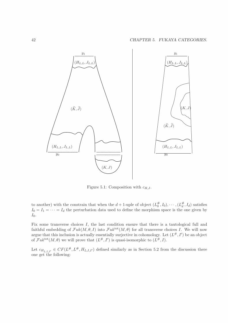
We claim that such elements cK,J are c-units of Fuk(M,θ, I). For this note that the mapµ2L0,L0,L0

(· · · , cK,J) applied on a cord y is given by a count of curve shown on the left hand sideof Figure.

For gluing parameter sufficiently large, this reduce to count curves shown on the right hand sideof Figure which is a comparison map as described before. Since the comparison map does notdepend on the perturbation data, it induce the identity in homology and therefore cK,J is a c-unit.

5.3 Well definedness

We prove now that the quasi-equivalence class of Fuk(M,θ, I) do not depend on I. In order to doso we define the A∞-category Fuktot(M,θ) whose objects are pair (L#, I) where L# is an exactgraded Lagrangian and I is a transverse choices of strip-like end, Floer data and perturbationdata. The morphism space are define similarly as in Fuk(M,θ, I) using some compatible choicesof perturbation data (bearing in mind that the notion of strip-like might change from one object


(HL,L, JL,L)

(HL,L, JL,L)

(K, J)

(HL,L, JL,L)

(HL,L, JL,L)

(K, J)

(K, J)

(K, J)

y1 y1

y0 y0

Figure 5.1: Composition with cH,J .

to another) with the constrain that when the d+ 1-uple of object (L#0 , I0), · · · , (L

#d , Id) satisfies

I0 = I1 = · · · = Id the perturbation data used to define the morphism space is the one given byI0.

Fix some transverse choices I, the last condition ensure that there is a tautological full andfaithful embedding of Fuk(M,θ, I) into Fuktot(M,θ) for all transverse choices I. We will nowargue that this inclusion is actually essentially surjective in cohomology. Let (L#, I ′) be an objectof Fuktot(M,θ) we will prove that (L#, I ′) is quasi-isomorphic to (L#, I).

Let cHL,I,I′∈ CF (L#, L#,HL,I,I′) defined similarly as in Section 5.2 from the discussion there

one get the following:

5.4. INVARIANCE 43

1. µ1(cH(L,I),(L,I′)) = 0

2. µ2(cH(L,I),(L,I′), cH(L,I′),(H,I)

) ∈ CF (L#, L#,H(L,I),(L,I)) is given by the count of curve shownin the left hand side of Figure which after gluing is given by the count of curve on the righthand side of Figure.

It follows from the second point and from Section 5.2 that µ2(cH(L,I),(L,I′), cH(L,I′),(H,I)

) is a c-unit

of CF (L#, L#,H(L,I),(L,I)) which means that in cohomology [cH(L,I),(L,I′)] [cH(L,I′),(H,I)

]. Thus

(L#, I) and (L#, I ′) are quasi-isomorphic. The inclusion functor being cohomologically full faith-ful and essentially surjective, one get that Fuk(M,θ, I) is quasi-isomorphic to Fuktot(M,θ) andtherefore given to choices I, I ′ the categories Fuk(M,θ, I) and Fuk(M,θ, I ′) are quasi-equivalent.Note that from the proof one can see that furthermore one can choose the quasi equivalence tosend object (L#, I) to (L′#, I ′) and thus one can now note those categories Fuk(M,θ) unam-biguously on objects.

5.4 Invariance

The goal of this section is to prove the following:

Theorem 5.4.1. Let (M,θ) and (M ′, θ′) be two exact symplectic manifolds such that there existsa diffeomorphisms φ : M → M ′ satisfying φ∗θ′ = θ + df then Fuk(M,θ) is quasi-equivalent toFuk(M ′, θ′).


Chapter 6

Some examples and some generation

criterion.

The goal of this chapter is to outline the geometric and algebraic idea behind Abouzaid’s gen-eration criterion in [Abo10] for Fukaya categories. We will be rather sketchy on the geometricalside and will assume that we are in a context where Lagrangian Floer homology is well definedand the symplectic manifold we consider is symplectically aspherical. It can however be compact(as we will see on our main example). The fact that we get out of the geometrical context is notproblematic on the algebraic part of the argument.

6.1 Biran-Cornea’s intersection criterion

A linear version of Abouzaid’s argument appears in [BC09, Theorem 2.4.1] where the followingis proved. Given two Lagrangian submanifolds L and K of (M,ω) (with (ω|π2(M) = 0) thereexists maps H∗(OC) : HF (L,L) → H∗(M) and H∗(CO) : H∗(M) → HF (K,K) such that ifH∗(CO) H∗(OC) 6= 0 then K ∩ L 6= ∅.

Roughly speaking, the maps H∗(OC) and H∗(CO) are defined using a Morse function on M acounting cardinality of the moduli spaces shown on Figure 6.1. In both case one should think thedomain of the curves to be a Riemann disk with one marked point on the boundary and one onthe interior and the equation interpolate between the perturbed Floer equation near the markedpoint on the boundary and the (positive or negative) gradient flow line equation near the markedpoint on the interior (a neighbourhood of which is identified with S1 × R± the equation being

45

46 CHAPTER 6. SOME EXAMPLES AND SOME GENERATION CRITERION.

independent of the S1 parameter).

γHL

L

q

L

q

L

γHL

∇f

∇f

Figure 6.1: Curve contributing to open-closed (< OCγHL, q > on the left) and closed-open

(< CO(q), γHL> on the right) maps (the arrow pointing on positive gradient direction).

We sketch here the argument to prove the theorem. Consider two curve contributing to theterm H∗(CO) H∗(OC) 6= 0 and glue them, the gluing curve belong to a 1-parameter family ofholomorphic annuli shown on Figure 6.2. As H∗(CO) H∗(OC) 6= 0 such family cannot breakto another pair of similar curve. The other possible breaking is depicted on Figure 6.2(onecannot have boundary bubbling or interior bubbling since the Lagrangian are exact and M issimplectically aspherical). Note that the marked points all along are 1 and −1 as this is discussedin [Abo10, Appendix C.4] in order to ensure the existence of relevant rigid moduli spaces. Fromthe position of the boundary marked points we deduce from the existence of such a breaking thatthere are intersection points between L and K.

Note that in the definition of the maps H∗(CO) and H∗(OC) no intersection points between L andK are involved so the existence of the intersection points are really detected from the algebraicmaps.

6.2 Toward Abouzaid’s criterion

The idea behind Abouzaid’s criterion is the following: if the identity maps in HF (K,K) isdecomposed as e = fn · · · f0 where fn ∈ HF (Ln,K), fi ∈ HF (Li, Li+1) and f0 ∈ HF (K,L1)

6.2. TOWARD ABOUZAID’S CRITERION 47

Figure 6.2: One dimensional family of annuli and its boundary. Stretching along the green lineleads to the breaking on the left and along the blue on leads to the one on the right.

then K is in the split closed triangulated category generated by ∪Li. To convince ourselvesthat it is necessary to take split closure (and not only triangulated) remark that if id = f gwhere f : V → W and g : W → V then g f is an idempotent which project V to a sub-objectof V isomorphic to W .

Going back to Biran-Cornea’s result the second type of breaking shows to type of map: one map∆ : HF∗(L,L) → HF∗(L,K)⊗HF∗(K,L) → HF∗(L,L) and second one which is the compositionµ2 : HF∗(K,L) ⊗ HF∗(L,K) → HF∗(K,K). The degeneration of the moduli space of annuliimplies that the following diagram commutes in homology:

HF∗(L,L)∆

//

H∗(OC)

HF∗(K,L) ⊗HF∗(L,K)

µ2

H∗(M)H∗(CO)

// HF (K,K)

(6.1)

The proof of the intersection criterion reads now as if H∗(CO) H∗(OC) 6= 0 then µ2 ∆ 6= 0 andthus HF∗(K, l) 6= 0 which implies the existence of intersection between K and L. Going furthertoward algebraic non-sense we can state the following proposition which is the linear version ofthe criterion we will state in the next section, it appears in [Smi14, Section 4.6.2].


Proposition 6.2.1. If the unit e ∈ HF (K,K) is in the image of H∗(CO) H∗(OC) then K isin the split-closure of the sub-category generated by L.

Proof. The hypothesis of the theorem and the commutativity of diagram (6.1) implies that e =∑µ2(pi, qi) for some pi ∈ HF (K,L) and qi ∈ HF (L,K). It suffices now to note that the maps

α : ⊕iHF (L,L) → HF (L,K) given by µ2(pi, ·) and β : HF (L,K) → ⊕iHF (L,L) given byβ = (µ2(q1, ·), . . . , µ2(qk, ·)) satisfy α β = Id and thus β α is a projector of ⊕HF (L,L) withimage isomorphic to HF (L,K). In terms of Yoneda’s embedding this implies that Y(K) is quasi-isomorphic to a sub-object of ⊕k−1

i=1 ⊗Y(L), by definition of being in the split closure, this impliesthat K is in the split closure of the subcategory generated by L.

6.3 Geometric criterion

The idea of the geometric criterion is to find a geometric argument which guarantees that theunit is in the image of the composition. First note that both H ∗ (M) and HF (K,K) are ringand that the map H∗(CO) is a unital ring morphism it therefore maps the unit to the unit sothat it suffices to check that the unit of H∗(M) is hit by the map H∗(OC).

This is however very unlikely to be the case as this would implies that the Fukaya category isgenerated by a single object L which is seldom the case. However one can consider a familyof object L1, . . . , Lk and add more marked point to define a map (on the chain level) OC :HC(B,B) → C∗(M,f) where B is the subcategory of Fuk(M) generated by the objects Li

ki=1

and HC(B,B) is the Hochschild complex of B with coefficient in B (seen as a bimodule overitself). That the domain is the Hochschild complex follows from the definition of the Hochschilddifferential and the degeneracies of one parameter family of disks with one marked point on theboundary.

Abouzaid’s criterion read now as the following

Theorem 6.3.1. (Abouzaid [Abo10] for the Wrapped Floer homology case, Abouzaid-Fukaya-Oh-Ohta-Ono for the closed and bulk Floer homology case) If the unit 1 ∈ H∗(M) is in the image ofH∗(OC) : HH∗(B,B) → H∗(M) then B split-generate the category Fuk(M).

In order to prove this theorem one must extend the previous commutative diagram to the nonlinear case of Hochschild homology. The map ∆ extend to a map from HC(B,B) to HC(B,Y l

K ⊗YrK). Algebraically this is just a change of coefficient in Hochschild homology and geometrically

this amount (roughly) to a count of of curves with two outgoing ends. Note that the Hochschildcomplex of B with coefficient in the bimodule Y l

K ⊗ YrK is isomorphic to the complex given by

6.3. GEOMETRIC CRITERION 49

C∗(YrK ⊗B Y l

K) (where ⊗B refer to the derived tensor product described in the algebraic partof the book) where the isomorphism is given by the map τ sending (a ⊗ b) ⊗ ad ⊗ · · · ⊗ a1where (a ⊗ b) ∈ Y l

K ⊗ YrK(L0, Ld) = hom(K,L0) ⊗ hom(Ld,K) and ai ∈ hom(Li−1, Li) to

b⊗ ad ⊗ · · · ⊗ a1 ⊗ a in hom(Ld,K)⊗ hom(Ld−1, Ld)⊗ · · · ⊗ hom(K,L0) which is a summand ofYrK ⊗B Y l

K .

In order to familiarised the reader with definition of Yoneda’s module and Hochschild differentialof the algebraic part of the book we encourage him to solve the following easy exercise.

Exercise 6.3.1. Show that τ is a chain map.

The maps µ2 of the previous section extend naturally to the map µ : C∗(YrK⊗BY

lK) → CF (K,K)

given by the compositions µdd.

The extension of the previous commutative diagram reads now as the following

Theorem 6.3.2. [Abo10, Proposition 1.3] The following diagram commutes in homology:

HC∗(B,B)∆

//

OC

C∗(YrK ⊗B Y l

K)

µ

C∗(M,f)CO

// CF∗(K,K)

. (6.2)

The hypothesis of Theorem 6.3.1 (and because H∗(CO) maps the unit to the unit) thereforeimplies that the unit of HF∗(K,K) is in the image of H∗(µ) for all object K of Fuk(M). Theproof of the Theorem 6.3.1 is completed once one prove the following:

Proposition 6.3.3. If e ∈ HF (K,K) is in the image of H∗(µ) then the Yoneda module YrK of

K is an idempotent image in a twisted complex over B.

Proof. Recall that the complex YrK⊗BY

lK is

⊕k

⊕X0,...Xk∈B

hom(Xk,K)⊗hom(Xk−1,Xk)⊗· · ·⊗hom(K,X0) with the obvious differential given by partial composition of the terms. Since e is inthe image of H∗(µ) there exist an N such that e in the image of the maps induced in homology bythe composition

⊕k≤N

⊕X0,...Xk∈B

hom(Xk,K)⊗hom(Xk−1,Xk)⊗· · ·⊗hom(K,X0) ⊂ C∗(YrK⊗B

Y lK) → CF (K,K).

Consider UNK the twisted complex over B given by UN

K =⊕

k≤N

⊕X0,...Xk∈B

hom(Xk,K) ⊗hom(Xk−1,Xk)⊗· · ·⊗Yr

X0with the differential given by all possible partial multiplication of the

terms. There is a full composition map f which maps UNK to Yr

K .


Note that the A∞ version of Yoneda’s lemma implies that hommod(UNk ,Y

rK) ≃ Ur

N (K) = (YrK ⊗B

Y lK)≤N :=

⊕k≤N

⊕X0,...Xk∈B

hom(Xk,K)⊗hom(Xk−1,Xk)⊗· · ·⊗hom(K,X0) and contemplatethe following (tautologically) commutative diagram

hommod(UNk ,Y

rK)

≃

f// hommod(Y

rK ,Y

rK)

≃

(YrK ⊗B Y l

K)≤Nµ

// hom(K,K)

(6.3)

We get that Id ∈ hommod(YrK ,Y

rK) is in the image of the composition maps : hommod(U

Nk ,Y

rK)⊗

hommod(YrK ,U

NK ) since e is in the image of µ.

The same argument as in the proof 6.2.1 implies that YrK is a split summand of some

⊕i U

NK

which by definition implies that K is in the split-closure of B.

6.4 Example

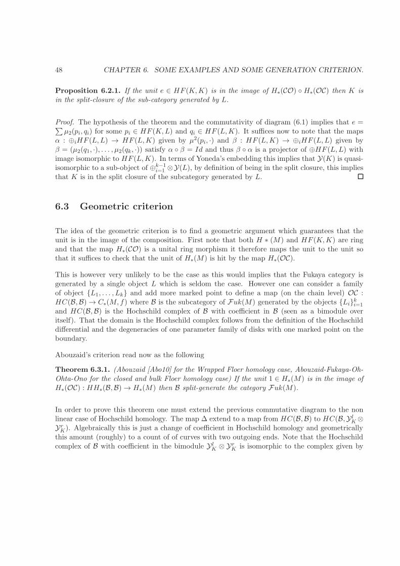
In order to give a (non rigorous) illustration of this criterion let’s try to understand how can wedetermine if the unit is in the image of H∗(OC). The unit of H∗(M) being represented in theMorse complex by the minimum m out which no rigid gradient flow line exits we get that thenumber < ad ⊗ a0,m > is given by a count of rigid holomorphic disks shown in Figure 6.3.

Figure 6.3: A rigid curve contributing to

Hence if one can find a family of object L such that for any generic point of m there is a

6.4. EXAMPLE 51

“unique” holomorphic disks passing through this point with boundary on L then we get thatH∗(OC)(ad,⊗, a0) = m where a0, . . . , ad are the corner of the unique disk passing through m.

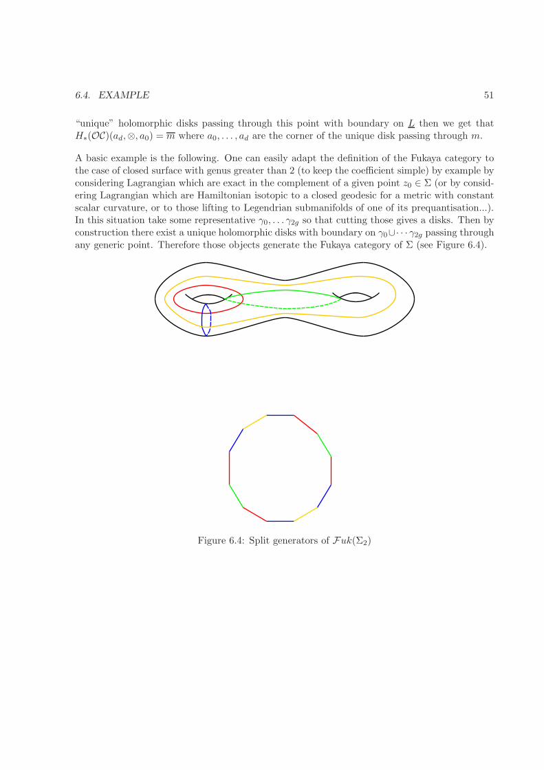
A basic example is the following. One can easily adapt the definition of the Fukaya category tothe case of closed surface with genus greater than 2 (to keep the coefficient simple) by example byconsidering Lagrangian which are exact in the complement of a given point z0 ∈ Σ (or by consid-ering Lagrangian which are Hamiltonian isotopic to a closed geodesic for a metric with constantscalar curvature, or to those lifting to Legendrian submanifolds of one of its prequantisation...).In this situation take some representative γ0, . . . γ2g so that cutting those gives a disks. Then byconstruction there exist a unique holomorphic disks with boundary on γ0∪· · · γ2g passing throughany generic point. Therefore those objects generate the Fukaya category of Σ (see Figure 6.4).

Figure 6.4: Split generators of Fuk(Σ2)


Bibliography

[Abo08] Mohammed Abouzaid. On the Fukaya categories of higher genus surfaces. Adv. Math.,217(3):1192–1235, 2008.

[Abo10] Mohammed Abouzaid. A geometric criterion for generating the Fukaya category. Publ.Math. Inst. Hautes Etudes Sci., (112):191–240, 2010.

[BC09] Paul Biran and Octav Cornea. Rigidity and uniruling for Lagrangian submanifolds.Geom. Topol., 13(5):2881–2989, 2009.

[Con95] John B. Conway. Functions of one complex variable. II, volume 159 of Graduate Textsin Mathematics. Springer-Verlag, New York, 1995.

[GH78] Phillip Griffiths and Joseph Harris. Principles of algebraic geometry. Wiley-Interscience[John Wiley & Sons], New York, 1978. Pure and Applied Mathematics.

[Gro85] M. Gromov. Pseudo holomorphic curves in symplectic manifolds. Invent. Math.,82(2):307–347, 1985.

[KS01] Maxim Kontsevich and Yan Soibelman. Homological mirror symmetry and torus fibra-tions. In Symplectic geometry and mirror symmetry (Seoul, 2000), pages 203–263. WorldSci. Publ., River Edge, NJ, 2001.

[Lod04] Jean-Louis Loday. Realization of the Stasheff polytope. Arch. Math. (Basel), 83(3):267–278, 2004.

[MS04] Dusa McDuff and Dietmar Salamon. J-holomorphic curves and symplectic topology,volume 52 of American Mathematical Society Colloquium Publications. American Math-ematical Society, Providence, RI, 2004.

[Rud87] Walter Rudin. Real and complex analysis. McGraw-Hill Book Co., New York, thirdedition, 1987.

53

54 BIBLIOGRAPHY

[Sei08] Paul Seidel. Fukaya categories and Picard-Lefschetz theory. Zurich Lectures in AdvancedMathematics. European Mathematical Society (EMS), Zurich, 2008.

[Smi14] I. Smith. A symplectic prolegomenon. ArXiv e-prints, January 2014.

[Sta63] James Dillon Stasheff. Homotopy associativity of H-spaces. I, II. Trans. Amer. Math.Soc. 108 (1963), 275-292; ibid., 108:293–312, 1963.

Index

Associahedra, 9

Pointed disk, 12

Semi-stabletree, 9

Stabletree, 9

Strip-like ends, 12consistent choice of, 14

Universal Riemann curve, 12

55

Documents

AnintroductiontoFukayacategories - Université de Nanteschantraine-b/fr/FukayaCategory.pdf · Introduction. This notes serve as a support for a Master2 class given in Universit de