Embed Size (px)
Citation preview

8/12/2019 Animation Cartography - Intrinsic Reconstruction of Shape and Motion
http://slidepdf.com/reader/full/animation-cartography-intrinsic-reconstruction-of-shape-and-motion 1/15
Animation Cartography—Intrinsic Reconstructionof Shape and Motion
ART TEVS, ALEXANDER BERNER, MICHAEL WAND, IVO IHRKE,
MARTIN BOKELOH, JENS KERBER, and HANS-PETER SEIDELMax-Planck Institut Informatik, and Saarland University
In this article, we consider the problem of animation reconstruction, that is,
thereconstructionof shape andmotion ofa deformable object from dynamic
3D scanner data, without using user-provided template models. Unlike pre-
vious work that addressedthis problem, we donot rely onlocally convergent
optimization but present a system that can handle fast motion, temporally
disrupted input, and can correctly match objects that disappear for extended
time periods in acquisition holes due to occlusion. Our approach is moti-
vated by cartography: We first estimate a few landmark correspondences,
which are extended to a dense matching and then used to reconstruct ge-
ometry and motion. We propose a number of algorithmic building blocks: a
scheme for tracking landmarks in temporally coherent and incoherent data,
an algorithm for robust estimation of dense correspondences under topo-
logical noise, and the integration of local matching techniques to refine the
result. We describe and evaluate the individual components and propose a
complete animation reconstruction pipeline based on these ideas. We eval-
uate our method on a number of standard benchmark datasets and show
that we can obtain correct reconstructions in situations where other tech-
niquesfail completelyor require additionaluser guidance such as a template
model.
Categories and Subject Descriptors: I.3.7 [Computer Graphics]: Three-
Dimensional Graphics and Realism— Animation; I.4.8 [Image Processing
and Computer Vision]: Scene Analysis—Surface fitting
General Terms: Algorithms, Design
Additional Key Words and Phrases: Registration, a nimation reconstruction,
dynamic 3D scanners
This work has been partially supported by the DFG “Cluster of Excellence
Multi-Modal Computing and Interaction.”
Authors’ addresses: A. Tevs (corresponding author), A. Berner, M. Wand,
I. Ihrke, M. Bokeloh, J. Kerber, and H.-P. Seidel, Max-Planck Institut Infor-
matik and Saarland University, Saarbrucken, Germany; email: tevs@mpi-
inf.mpg.de.
Permission to make digital or hard copies of part or all of this work for
personal or classroom use is granted without fee provided that copies are
not made or distributed for profit or commercial advantage and that copies
show this notice on the first page or initial screen of a display along with
the full citation. Copyrights for components of this work owned by othersthan ACM must be honored. Abstracting with credit is permitted. To copy
otherwise, to republish, to post on servers, to redistribute to lists, or to use
anycomponent of this work in otherworks requires prior specific permission
and/or a fee. Permissions may be requested from Publications Dept., ACM,
Inc., 2 Penn Plaza, Suite 701, New York, NY 10121-0701 USA, fax +1
(212) 869-0481, or [email protected].
c 2012 ACM 0730-0301/2012/04-ART12 $10.00
DOI 10.1145/2159516.2159517
http://doi.acm.org/10.1145/2159516.2159517
ACM Reference Format:
Tevs, A.,Berner, A.,Wand,M., Ihrke, I.,Bokeloh, M.,Kerber, J.,and Seidel,
H.-P. 2012. Animation cartography—Intrinsic reconstruction of shape and
motion. ACM Trans. Graph. 31, 2, Article 12 (April 2012), 15 pages.
DOI = 10.1145/2159516.2159517
http://doi.acm.org/10.1145/2159516.2159517
1. INTRODUCTION
Recently, a number of techniques have been proposed to scan three-dimensional moving objects in real time [Wurmlin et al. 2002;Zhang et al. 2004; Zitnick et al. 2004; Davis et al. 2005; Weiseet al. 2007; Konig and Gumhold 2008; Vlasic et al. 2009; Bradleyet al. 2010]. The output of such an acquisition process is a sequenceof unstructured point clouds. The measurement process does notprovide any correspondence information and usually only shows alimited part of theobject ata time, dueto occlusions.This introducesa new problem, the problem of animation reconstruction: How canwe reconstruct the shape and the motion of a deformable objectgiven that only parts of it can be seen at any given point in time?More precisely, we want to reconstruct the full shape out of thepartial observations and establish dense correspondences over timethat describe the motion of the object.
Some techniques have recently been proposed to solve thisproblem [Mitra et al. 2007; Wand et al. 2007, 2009; Pekelny and
Gotsman 2008; Sußmuth et al. 2008]. However, these approachesemploy local numerical optimization to align parts of the object in-crementally: The final shape is inferred by a deformable alignmentof the geometry in time sequence order. If some of the alignmentsyield an incorrect result, neither the shape of the deformable objectnor the correspondences are reconstructed correctly. In practice,alignment problems are frequently observed. They are caused byfast object movement or vanishing geometry that reappears in laterframesin a differentpose. Localalignment isnot able tohandle thesesituations correctly. The problem obviously becomes much easier if the user provides additional information, such as a template model[Carranza et al. 2003; Sand et al. 2003; Anuar and Guskov 2004;Zhang et al. 2004; Park and Hodgins 2006; de Aguiar et al. 2008;Li et al. 2009]. Nevertheless, numerical tracking can still fail sothat manual user intervention becomes necessary. Furthermore, the
fixed template restricts the expressiveness of the model, prohibitstopological changes, and makes an acquisition of general scenestedious.
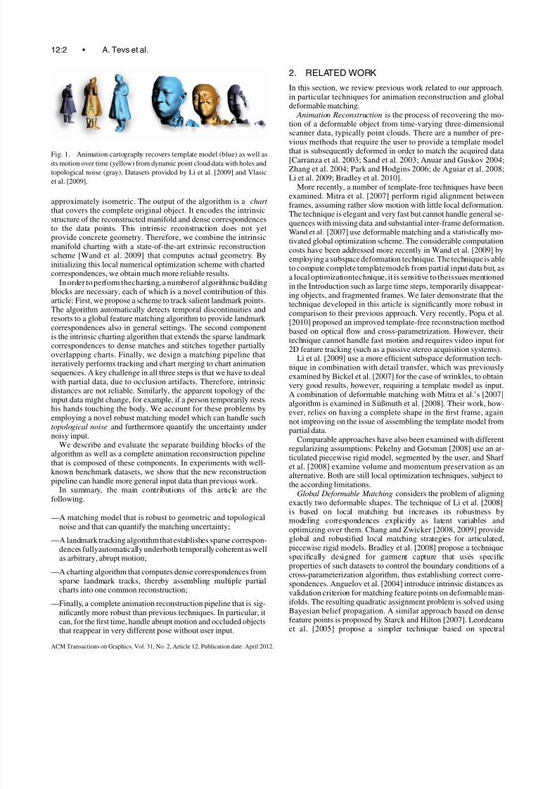
We present a template-free technique (Figure 1) that is ableto assemble shapes from partial scans more robustly and undergeneral motion than previous methods. The main idea is motivatedby cartography (from which we derive the name of the approach,animation cartography). We first track the location of a fewlandmark points, which we subsequently use to compute densecorrespondences, assuming that the deformation of the object is
ACM Transactions on Graphics, Vol. 31, No. 2, Article 12, Publication date: April 2012.
8/12/2019 Animation Cartography - Intrinsic Reconstruction of Shape and Motion
http://slidepdf.com/reader/full/animation-cartography-intrinsic-reconstruction-of-shape-and-motion 2/15
12:2 • A. Tevs et al.
Fig. 1. Animation cartography recovers template model (blue) as well as
its motion over time (yellow) from dynamic point cloud data with holes and
topological noise (gray). Datasets provided by Li et al. [2009] and Vlasic
et al. [2009].
approximately isometric. The output of the algorithm is a chart that covers the complete original object. It encodes the intrinsicstructure of the reconstructed manifold and dense correspondencesto the data points. This intrinsic reconstruction does not yetprovide concrete geometry. Therefore, we combine the intrinsicmanifold charting with a state-of-the-art extrinsic reconstructionscheme [Wand et al. 2009] that computes actual geometry. Byinitializing this local numerical optimization scheme with charted
correspondences, we obtain much more reliable results.In order to perform thecharting, a numberof algorithmic buildingblocks are necessary, each of which is a novel contribution of thisarticle: First, we propose a scheme to track salient landmark points.The algorithm automatically detects temporal discontinuities andresorts to a global feature matching algorithm to provide landmark correspondences also in general settings. The second componentis the intrinsic charting algorithm that extends the sparse landmark correspondences to dense matches and stitches together partiallyoverlapping charts. Finally, we design a matching pipeline thatiteratively performs tracking and chart merging to chart animationsequences. A key challenge in all three steps is that we have to dealwith partial data, due to occlusion artifacts. Therefore, intrinsicdistances are not reliable. Similarly, the apparent topology of theinput data might change, for example, if a person temporarily restshis hands touching the body. We account for these problems byemploying a novel robust matching model which can handle suchtopological noise and furthermore quantify the uncertainty undernoisy input.
We describe and evaluate the separate building blocks of thealgorithm as well as a complete animation reconstruction pipelinethat is composed of these components. In experiments with well-known benchmark datasets, we show that the new reconstructionpipeline can handle more general input data than previous work.
In summary, the main contributions of this article are thefollowing.
—A matching model that is robust to geometric and topologicalnoise and that can quantify the matching uncertainty;
—A landmark tracking algorithm that establishes sparse correspon-
dences fullyautomatically underboth temporally coherent as wellas arbitrary, abrupt motion;
—A charting algorithm that computes dense correspondences fromsparse landmark tracks, thereby assembling multiple partialcharts into one common reconstruction;
—Finally, a complete animation reconstruction pipeline that is sig-nificantly more robust than previous techniques. In particular, itcan, for the first time, handle abrupt motion and occluded objectsthat reappear in very different pose without user input.
2. RELATED WORK
In this section, we review previous work related to our approach,in particular techniques for animation reconstruction and globaldeformable matching.
Animation Reconstruction is the process of recovering the mo-tion of a deformable object from time-varying three-dimensionalscanner data, typically point clouds. There are a number of pre-vious methods that require the user to provide a template modelthat is subsequently deformed in order to match the acquired data[Carranza et al. 2003; Sand et al. 2003; Anuar and Guskov 2004;Zhang et al. 2004; Park and Hodgins 2006; de Aguiar et al. 2008;Li et al. 2009; Bradley et al. 2010].
More recently, a number of template-free techniques have beenexamined. Mitra et al. [2007] perform rigid alignment betweenframes, assuming rather slow motion with little local deformation.The technique is elegant and very fast but cannot handle general se-quences with missing data and substantial inter-frame deformation.Wand et al. [2007] use deformable matching and a statistically mo-tivated global optimization scheme. The considerable computationcosts have been addressed more recently in Wand et al. [2009] byemploying a subspace deformation technique. The technique is ableto compute complete templatemodels from partial input data but, as
a local optimizationtechnique, it is sensitive to theissues mentionedin the Introduction such as large time steps, temporarily disappear-ing objects, and fragmented frames. We later demonstrate that thetechnique developed in this article is significantly more robust incomparison to their previous approach. Very recently, Popa et al.[2010] proposed an improved template-free reconstruction methodbased on optical flow and cross-parametrization. However, theirtechnique cannot handle fast motion and requires video input for2D feature tracking (such as a passive stereo acquisition systems).
Li et al. [2009] use a more efficient subspace deformation tech-nique in combination with detail transfer, which was previouslyexamined by Bickel et al. [2007] for the case of wrinkles, to obtainvery good results, however, requiring a template model as input.A combination of deformable matching with Mitra et al.’s [2007]algorithm is examined in Sußmuth et al. [2008]. Their work, how-
ever, relies on having a complete shape in the first frame, againnot improving on the issue of assembling the template model frompartial data.
Comparable approaches have also been examined with differentregularizing assumptions: Pekelny and Gotsman [2008] use an ar-ticulated piecewise rigid model, segmented by the user, and Sharf et al. [2008] examine volume and momentum preservation as analternative. Both are still local optimization techniques, subject tothe according limitations.
Global Deformable Matching considers the problem of aligningexactly two deformable shapes. The technique of Li et al. [2008]is based on local matching but increases its robustness bymodeling correspondences explicitly as latent variables andoptimizing over them. Chang and Zwicker [2008, 2009] provideglobal and robustified local matching strategies for articulated,piecewise rigid models. Bradley et al. [2008] propose a techniquespecifically designed for garment capture that uses specificproperties of such datasets to control the boundary conditions of across-parameterization algorithm, thus establishing correct corre-spondences. Anguelov et al. [2004] introduce intrinsic distances asvalidation criterion for matching feature points on deformable man-ifolds. The resulting quadratic assignment problem is solved usingBayesian belief propagation. A similar approach based on densefeature points is proposed by Starck and Hilton [2007]. Leordeanuet al. [2005] propose a simpler technique based on spectral
ACM Transactions on Graphics, Vol. 31, No. 2, Article 12, Publication date: April 2012.

8/12/2019 Animation Cartography - Intrinsic Reconstruction of Shape and Motion
http://slidepdf.com/reader/full/animation-cartography-intrinsic-reconstruction-of-shape-and-motion 3/15
Animation Cartography—Intrinsic Reconstruction of Shape and Motion • 12:3
relaxation for solving quadraticfeature assignment problems,whichhas been employed for isometric matching by Huang et al. [2008]and Ahmed et al. [2008]. The two papers introduce landmark coor-dinates for deriving densematchesfrom the coarse matches returnedby spectral matching, a concept that has previously been inventedin the context of routing in sensor networks [Fang et al. 2005].
A problem with all these intrinsic matching strategies is topolog-
ical noise: Acquisition holes as well as apparent topology changes,such as a closing mouth in a face scan, might strongly distort intrin-sic distances such that correspondences cannot be detected reliably.Bronstein et al. [2009] address this problem by mixing geodesicand Euclidean distances, but this solves the problem only in somecases. In general, both extrinsic and intrinsic distances mightbe verydifferent. In addition, the technique is based on local numerical op-timization, which requires prealignment of the data. More recently,Bronstein et al. [2010] propose diffusion distances, which are morerobust to a certain amount of topological noise, as this distancemeasure is sensitive to the cross-section of interconnections ratherthan just the reachability in the case of geodesic distances.However,large-scale artifacts such as big acquisition holes or false connec-tions in a large area also change diffusion distances significantly.Unfortunately, these problems are common in our application area(large acquisition holes, arms at the body, closing mouth in a facescan, etc.).
Tevs et al. [2009] address this problem in a different way by al-lowing for outlier geodesic distances within a RANSAC algorithm.This approach requires a minimum set of “witness geodesics” butotherwise does not depend on the geometric extent of topologi-cal noise. We put their technique on a sound statistical basis thatallows for explicitly calculating matching uncertainties. More im-portantly, Tevs et al. [2009] are limited to pairwise matching whilewe address the more general problem of simultaneously recon-structing 3D topology and correspondences over long sequences.The reconstruction of many-frame correspondences is a nontrivialgeneralization: Just repeatedly performing pairwise matches expo-nentially increases the failure probability of randomized matching,thus rendering merging of long sequences practically impossible.We avoid this pitfall by on the one hand using a continuous tracking
algorithm to detect and use local temporal coherence and on theother hand by explicitly assessing the matching quality, avoidingthe incorporation of ambiguous information in the result.
Global Animation Reconstruction refers to methods that aimat incorporating more information than pairwise matching canprovide into the reconstruction process. The previously cited globalregistration methods only consider, with the exception of Ahmedet al. [2008] and Varanasi et al. [2008], the pairwise matching case.Their methods are based on matching feature distances computed byLaplacian diffusion which is not robust against general topologicalnoise. In addition, both methods require color information asso-ciated with the point cloud data for matching SIFT/SURF featuresand thus cannot be applied to purely geometric datasets. The sameholds for the technique of Liao et al. [2009], which also does notaddress the problem of handling temporal gaps or jumps in motion
where continuous tracking breaks down. The method of Popaet al. [2010] also requires image information. It performs intrinsiccross-parametrization, similar to our approach, but has to assumea “gradual change” prior (rather than robust matching densities)to resolve ambiguities, therefore not yet providing a full globalanimation reconstruction. A very interesting, recent approach byZheng et al. [2010] aims at reconstructing the temporal correspon-dences of a skeleton rather than complete geometry, which can thensubsequently be used as guidance information for shape alignment.The drawback in comparison to our approach is that although
skeletonization improves robustness, it does not represent the fullcorrespondence information, which cannot always be recoveredreliably.
3. OVERVIEW
We start with an introduction of concepts that are used through-
out the rest of the article: We first formally define the problemthat we are solving and describe the input data we are expecting(Section 3.1). Next, we describe the data structures that we use torepresent charts, and how intrinsic and extrinsic information is rep-resented (Section 3.2). Afterwards, we describe the robust matchingmodel that is used throughout the article (Section 3.3). Finally, weconclude this section with an overview of the individual reconstruc-tion steps and how they are combined in the final reconstructionpipeline (Section 3.4).
3.1 Problem Statement
Original animations. The goal of our method is to reconstruct amanifold and its motion from partial observations. Formally, weassume that there has been an original differentiable 2-manifoldM ⊂ R
3 that underwent a time-variant motion f t : M → R3.
t ∈ [1, T ] is the time parameter. Each f t is assumed to be injectiveand differentiable, and each f t (M) denotes a deformed version of the original manifold M.
Isometry assumption. We equip differentiable manifolds M ⊂
R3 with an intrinsic metric d M(·, ·) that measures the shortest
geodesic distance between pairs of points. We assume that the de-formationf t is approximately isometric for each fixed t . This meansthat
∀t ∈ {1..T } : d M(x, y) = d f t (M) (f t (x), f t (y)) + ησ f , (1)
where ησ f ∼ N (0, σ f ) is an error that is normal distributed withstandard deviation σ f and mean zero. In other words, we assumethat the original deformation, even before measurement, has notbeen perfectly isometric but that there might have been errors thatare in the range of σ f .
Discussion. Assuming (approximate) isometry is an establishedmodel [Anguelov et al. 2004; Bronstein et al. 2006; Bradley et al.2008]. It is sufficiently general to characterize the motion of thesurface of manyreal-world objects,such as scans of people, animals,plants, or clothing. A strongly nonisometric surface deformationwould be fatal to suchobjects.Nevertheless, intrinsicisometryposesa strong constraint on the interpretation of observed data; one canthinkof a rigidityassumption within the manifold(rather thanwithinthe embedding space). Consequently, isometries have only veryfew degrees of freedom once the manifold they act upon is known[Lipman and Funkhouser 2009; Ovsjanikov et al. 2010; Tevs et al.2011].
Measurement. A 3D scanner only yields a partial, sampled rep-resentation. We assume that the scanner operates at regular timesteps t ∈ {1, 2, . . . , T } and for each time step, yields a finite set
of sample points Dt ⊂ R
3
. We denote the individual points byd
(i)t , i = 1, . . . , nt and the collection of all input data by just D.
To simplify further processing, we assume that parts of objects thathave actually been acquired have been sampled with a sample spac-ing ofat mosts , that is,for each point of theoriginalsurface visibleby the 3D scanner, there is a sample point in Euclidean distance of at most s . Areas with lower sampling density are discarded duringpreprocessing. Furthermore, we assume that all of M at some pointhas been observed with sufficient sampling density (or equivalently,we only try to reconstruct what we have observed).
ACM Transactions on Graphics, Vol. 31, No. 2, Article 12, Publication date: April 2012.
8/12/2019 Animation Cartography - Intrinsic Reconstruction of Shape and Motion
http://slidepdf.com/reader/full/animation-cartography-intrinsic-reconstruction-of-shape-and-motion 4/15
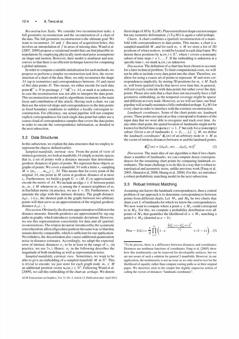
12:4 • A. Tevs et al.
Reconstruction Tasks. We consider two reconstruction tasks: afull geometric reconstruction and the reconstruction of a chart of the data. The full geometric reconstruction is the ultimate goal: Wewant to reconstruct M and f . Because of acquisition holes, thisinvolves an interpolation of f in areas of missing data. Wand et al.[2007, 2009] propose a variational model that can find plausible in-terpolations by employing physically motivated prior assumptions
on shape and motion. However, their model is nonlinear and non-convex so that there is no efficient technique known for computinga global optimum.
In order to compute a suitable initialization for such methods, wepropose to perform a simpler reconstruction task first, the recon-struction of a chart of the data. Here, we only reconstruct the shapeM (up to isometries) and correspondences between M and (mostof the) data points D . This means, we either encode for each data
point d(i)t ∈ D its preimage f −1(d
(i)t ) ∈ M, or mark it as unknown,
in case the reconstruction was not able to interpret the data point.This reconstruction model and its algorithmic treatment is the mainfocus and contribution of this article. Having such a chart, we canthen use the retrieved shape and correspondences to the data pointsas fixed boundary conditions to stabilize a locally convergent re-construction. For efficiency, our actual pipeline will not computeexplicit correspondences for each single data point but rather use acoarse cloud of correspondence samples that covers the data pointsin order to encode the correspondence information, as detailed inthe next subsection.
3.2 Data Structures
In this subsection, we explain the data structures that we employ torepresent the objects defined earlier.
Sampled manifolds, intrinsic view. From the point of view of intrinsicgeometry,we look at manifoldsM simply as metric spaces,that is, a set of points with a distance measure that determinesgeodesic distances of pairs of points. We represent these objects asgraphs of points: We cover a manifoldM with a finite s-samplingM = {m1, . . . ,mnM } ⊂ M. This means that for every point of theoriginal M, one point in M exists at geodesic distance of at most
s . Furthermore, we build a graph G = (M, E) to approximatelyencode the metric of M. We include an edge e ∈ E between pointsmi, mj ∈ M whenever mj is among the k-nearest neighbors of miin Euclidian metric (in practice, we use k = 20). Furthermore, weannotate the edge with this intrinsic distance. The graph distanced M (·, ·) (i.e., the shortest path in the graph) between two arbitrarypoints will then serve as an approximation of the original geodesicdistance d M(·, ·).
Discussion. Obviously, the discrete approximation willdistort thedistance measure. Smooth geodesics are approximated by zig-zagpaths in graphs, which introduces systematic deviations. However,we use this representation consistently for data and all (partial)reconstructions. The relative deviation introduced by the systematicerrorstherefore affect allgeodesicpathsin thesame way so that theyremain directly comparable, which is sufficient for our application.
Nevertheless, the discretization also causes additional quantizationnoise in distance estimates. Accordingly, we adapt the expectederror of intrinsic distances σ f to be at least in the range of s (inpractice, we use 3s). Hence, σ f in the following describes themagnitude of both modeling as well as representation noise.
Sampled manifolds, extrinsic view. Sometimes, we want to beable to give an embedding of a sampled manifold M in R3. Thisis trivial to encode; we just store for each graph node mi ∈ M an additional position vector x0(mi) ∈ R
3. Following Wand et al.[2009], we call this embedding of the chart an urshape. We denote
theurshape of M byX0(M ). Pleasenotethaturshapes arenot uniquebut any isometric deformation f (X0(M )) is again a valid urshape.
Charts. A chart combines a (partial) reconstruction of a mani-fold with correspondences to data points. This means, a chart is asampled manifold M , and for each m i ∈ M we store a list of 3Dpositions of where nodemi would be located in each data frame.Wedenote these positions by xt (mi) ∈ R
3, where t covers a nonempty
subset of time steps t ∈ 1, . .,T . If the embedding is unknown at aspecific time t , we mark xt (mi) as unknown. Discussion. The definition of a chart has been chosen to account
for a later technical problem: To limit computational costs, we willnot be able to include every data point into the chart. Therefore, weallow for using a coarse set of points to represent M and store cor-respondences implicitly, by storing 3D positions for mi ∈ M . Eachmi will form (partial) tracks that move over time but, in general,will not exactly coincide with data points but rather cover the datapoints. Please also note that a chart does not necessarily have a fullgeometric embedding, as the temporal coverage might be sparseand different at every node. However, as we will see later, our finalpipeline will actually maintain a fully embedded urshapeX0(M ) forevery chart in order to interface with the extrinsic reconstruction.
Landmark coordinates. Some of the chart points are landmark points. These points are special as they correspond to features of theinput data that we were able to recognize and track over time. Asany other chart point, the spatial location of landmarks might not beknown for thefull time sequence t = 1..T but only for a (nonempty)subset. Given a set of landmarks L = {l1, . ., ln} ⊆ M , we definethe landmark coordinates1 dL(m) of an arbitrary node m ∈ M asthe vector of intrinsic distances betweenm and the landmark points.
d(L)M (m) = [d M (l1,m), . .,d M (ln, m)]T (2)
Discussion. The main idea of our algorithm is that if two chartsshare a number of landmarks, we can compute dense correspon-dences for the remaining chart points by comparing landmark co-ordinates. The main challenge is to do this in a way that is robust totopological and geometric noise, unlike previous work [Fang et al.2005; Ahmed et al. 2008; Huang et al. 2008]. For this, we introducea robust probabilistic matching model in the next subsection.
3.3 Robust Intrinsic Matching
Assuming one knows the landmark correspondences, then a centralproblem of our approach is to determine correspondences betweenpoints from different charts. Let M A and M B be two charts thatshare a set L of landmarks for which we know the correspondences.We now want to compute where a point a ∈ M A could correspondto in M B . For this, we compute a probability distribution over allpoints of M B that quantifies the likelihood of a ∈ M A matching apoint b ∈ M B (denoted as a ∼ b).
Pr(a ∼ b|L) =1
Z
|L|j =1
λ · e
−
d
(L)M A
(a)[j ]−d(L)M B
(b)[j ]
2
2σ 2f + (1 − λ)
, (3)
1To be precise, there is a difference between distances and coordinates:
Distances are nonlinear functions of coordinates. Fang et al. [2005] show
how this nonlinearity can be removed for developable surfaces, but we
are not aware of such a solution for general 2-manifolds. However, in our
application, the nonlinearity is not an issue as we only need to test for the
likelihood of equality rather than compute routing paths as in their original
paper. We therefore stick to the simple but slightly imprecise notion of
calling the vectors of distances “landmark coordinates”.
ACM Transactions on Graphics, Vol. 31, No. 2, Article 12, Publication date: April 2012.
8/12/2019 Animation Cartography - Intrinsic Reconstruction of Shape and Motion
http://slidepdf.com/reader/full/animation-cartography-intrinsic-reconstruction-of-shape-and-motion 5/15
Animation Cartography—Intrinsic Reconstruction of Shape and Motion • 12:5
high
low
reliable unreliable unreliable
graph A graph B
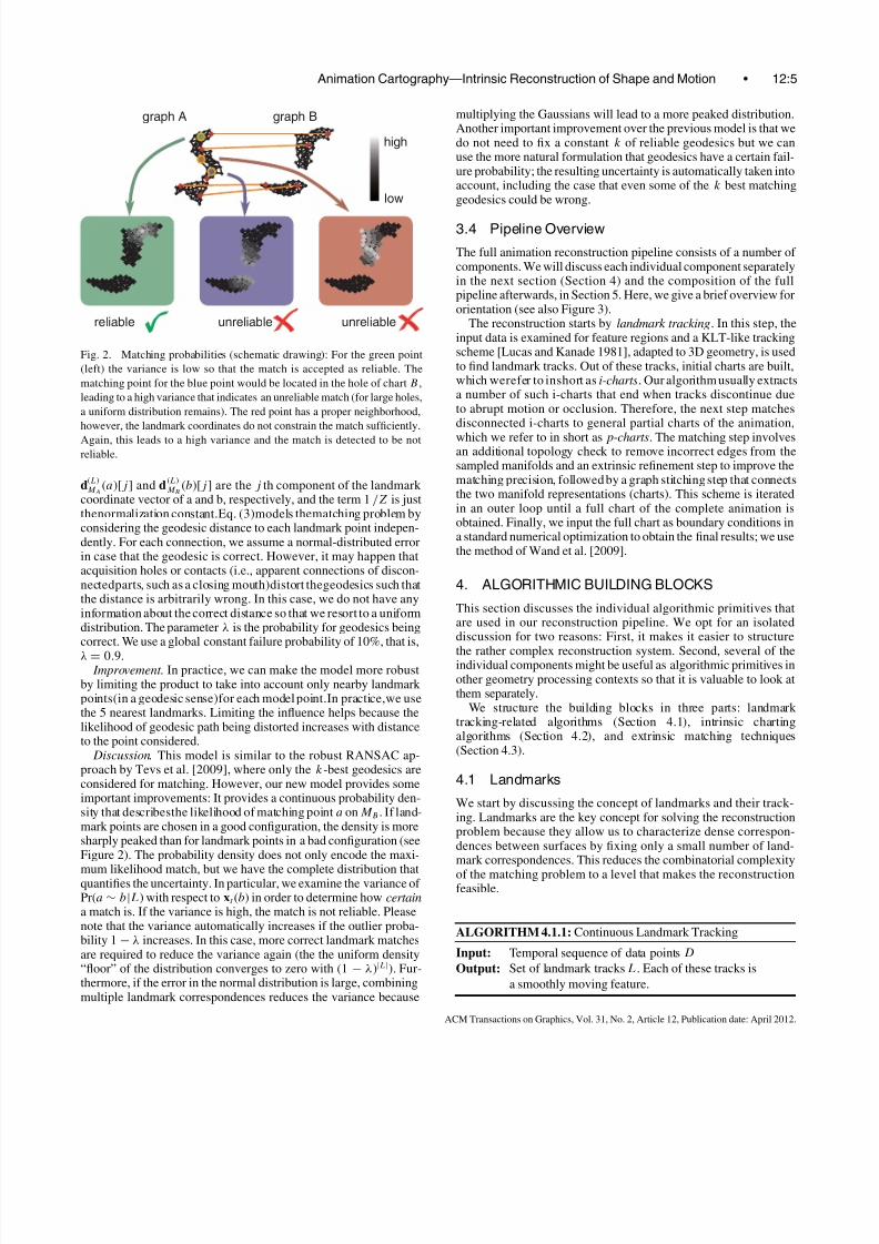
Fig. 2. Matching probabilities (schematic drawing): For the green point
(left) the variance is low so that the match is accepted as reliable. The
matching point for the blue point would be located in the hole of chart B ,
leading to a high variance that indicates an unreliable match (for large holes,
a uniform distribution remains). The red point has a proper neighborhood,
however, the landmark coordinates do not constrain the match sufficiently.
Again, this leads to a high variance and the match is detected to be not
reliable.
d(L)M A
(a)[j ] and d(L)M B
(b)[j ] are the j th component of the landmark coordinate vector of a and b, respectively, and the term 1/Z is justthenormalization constant.Eq. (3)models thematching problem byconsidering the geodesic distance to each landmark point indepen-dently. For each connection, we assume a normal-distributed errorin case that the geodesic is correct. However, it may happen thatacquisition holes or contacts (i.e., apparent connections of discon-nectedparts, such as a closing mouth)distort thegeodesics such thatthe distance is arbitrarily wrong. In this case, we do not have anyinformation about the correct distance so that we resort to a uniformdistribution. The parameter λ is the probability for geodesics beingcorrect. We use a global constant failure probability of 10%, that is,
λ = 0.9. Improvement. In practice, we can make the model more robust
by limiting the product to take into account only nearby landmark points(in a geodesic sense)for each model point.In practice,we usethe 5 nearest landmarks. Limiting the influence helps because thelikelihood of geodesic path being distorted increases with distanceto the point considered.
Discussion. This model is similar to the robust RANSAC ap-proach by Tevs et al. [2009], where only the k -best geodesics areconsidered for matching. However, our new model provides someimportant improvements: It provides a continuous probability den-sity that describesthe likelihood of matching point a onM B . If land-mark points are chosen in a good configuration, the density is moresharply peaked than for landmark points in a bad configuration (seeFigure 2). The probability density does not only encode the maxi-
mum likelihood match, but we have the complete distribution thatquantifies the uncertainty. In particular, we examine the variance of Pr(a ∼ b|L) with respect to xt (b) in order to determine how certaina match is. If the variance is high, the match is not reliable. Pleasenote that the variance automatically increases if the outlier proba-bility 1 − λ increases. In this case, more correct landmark matchesare required to reduce the variance again (the the uniform density“floor” of the distribution converges to zero with (1 − λ)|L|). Fur-thermore, if the error in the normal distribution is large, combiningmultiple landmark correspondences reduces the variance because
multiplying the Gaussians will lead to a more peaked distribution.Another important improvement over the previous model is that wedo not need to fix a constant k of reliable geodesics but we canuse the more natural formulation that geodesics have a certain fail-ure probability; the resulting uncertainty is automatically taken intoaccount, including the case that even some of the k best matchinggeodesics could be wrong.
3.4 Pipeline Overview
The full animation reconstruction pipeline consists of a number of components. We will discuss each individual component separatelyin the next section (Section 4) and the composition of the fullpipeline afterwards, in Section 5. Here, we give a brief overview fororientation (see also Figure 3).
The reconstruction starts by landmark tracking. In this step, theinput data is examined for feature regions and a KLT-like trackingscheme [Lucas and Kanade 1981], adapted to 3D geometry, is usedto find landmark tracks. Out of these tracks, initial charts are built,which werefer to inshort as i-charts. Our algorithm usually extractsa number of such i-charts that end when tracks discontinue dueto abrupt motion or occlusion. Therefore, the next step matchesdisconnected i-charts to general partial charts of the animation,
which we refer to in short as p-charts. The matching step involvesan additional topology check to remove incorrect edges from thesampled manifolds and an extrinsic refinement step to improve thematching precision, followed by a graph stitching step that connectsthe two manifold representations (charts). This scheme is iteratedin an outer loop until a full chart of the complete animation isobtained. Finally, we input the full chart as boundary conditions ina standard numerical optimization to obtain the final results; we usethe method of Wand et al. [2009].
4. ALGORITHMIC BUILDING BLOCKS
This section discusses the individual algorithmic primitives thatare used in our reconstruction pipeline. We opt for an isolateddiscussion for two reasons: First, it makes it easier to structure
the rather complex reconstruction system. Second, several of theindividual components might be useful as algorithmic primitives inother geometry processing contexts so that it is valuable to look atthem separately.
We structure the building blocks in three parts: landmark tracking-related algorithms (Section 4.1), intrinsic chartingalgorithms (Section 4.2), and extrinsic matching techniques(Section 4.3).
4.1 Landmarks
We start by discussing the concept of landmarks and their track-ing. Landmarks are the key concept for solving the reconstructionproblem because they allow us to characterize dense correspon-dences between surfaces by fixing only a small number of land-mark correspondences. This reduces the combinatorial complexity
of the matching problem to a level that makes the reconstructionfeasible.
ALGORITHM 4.1.1: Continuous Landmark Tracking
Input: Temporal sequence of data points D
Output: Set of landmark tracks L. Each of these tracks is
a smoothly moving feature.
ACM Transactions on Graphics, Vol. 31, No. 2, Article 12, Publication date: April 2012.

8/12/2019 Animation Cartography - Intrinsic Reconstruction of Shape and Motion
http://slidepdf.com/reader/full/animation-cartography-intrinsic-reconstruction-of-shape-and-motion 6/15
12:6 • A. Tevs et al.
Fig. 3. Overview of the animation cartography pipeline. Landmark tracks, Algorithm 4.1.1, are used to build initial charts (i-charts), Algorithm 4.2.1, which
are recursively combined in a pairwise chart merging loop, Algorithm 4.2.2–4.3.2. The final result is used to initialize a numerical bundle adjustment algorithmfor postprocessing. Dotted blocks indicate extrinsic matching components based on previous work of Wand et al. [2009]. A more detailed description of how
each of the part fits in the overall approach is given in Section 5.
The first component is a tracker for continuous landmark tracks.It gets the raw data D from the scanner as input. The task isto: (1) identify feature regions, (2) track features over time, and(3) recognize when tracks end due to incoherent motion.
We solve the first problem (1) by running slippage analy-sis [Gelfand and Guibas 2004]. It looks at every frame D t of the
data and determines for each point d(i)t whether a region of radius r
around d(i)t can be stably aligned to itself under a rigid motion (in
practice, we use r = 10% of the bounding box size of the object).For flat areas, for example, the alignment is unstable because the
patch could just slip along the plane. We keep only the unslippableregions and perform a coarse r-sampling to distribute feature pointsuniformly. Again, we use a Poisson-disc algorithm to obtain a gooduniform distribution.
The main tracking step (2) is performed by simple rigid ICP(Figure 4): We extract the r-neighborhood of each feature point andalign it to the next frame using point-to-plane ICP, always initializedto the (known) position of the previous frame. If the algorithmconverges, we align the same geometry again to the next frame, anditerate until the alignment diverges. The landmark track is givenby the trajectory of the center of the aligned region (the featurepoint) over time. Divergence is determined (3) by not convergingto a fixed point within 32 iterations or by a translational motionby more than r within one frame (which is likely to be wrong,because there was no initial overlap of the geometry with the newtarget).
We start new tracks automatically: For each new frame, we re-compute the nonslippable regions and insert a new point wheneverit is not r -covered with feature points that are being tracked.
Discussion. This scheme could be considered a geometric vari-ant of the well-known KLT feature tracker for images [Lucas andKanade 1981]. It works quite effectively in our situation becausescanned data usually contains a lot of coherent motion (but noteverywhere) with small motion between frames. Locally, within asmall spatial and temporal environment, the motion is usually al-most rigid. Our scheme does not lead to perfect results but mightcreate both false negatives and positives, which have to be handledby the robust matching model.
ALGORITHM 4.1.2: Connecting Broken Tracks
Input: Two points clouds A, B ⊂ R3, feature points F
A ∈ A.
Optionally: seed correspondences L between A and B .
Output: Correspondences between all a ∈ F A and points in B
(set to “unknown” if unreliable)
Usually, the tracking algorithm is not able to cover the wholeanimation sequence but rapid motion or occlusion disrupts someor all of the tracks. Therefore, we need an algorithm to reconnectbroken tracks.
Fig. 4. We align small patches of points to successive frames via ICP to
generate tracks. A track is stopped when ICPfails to compute a stable result.
We consider two point clouds A, B ⊂ R3. They might already
have a small number of landmark tracks L in common, but the setL can be empty. If a few continuous tracks are present, we includethese as initialization,so that thealgorithm finds thecorrect solutionmore quickly and more reliably. We now form candidate landmark correspondences by connecting each landmark node of A to everyother node inB (here:landmarks andordinarynodes). From this set,we have to find a consistent subset. We employ a forward searchalgorithm [Chum and Matas 2005; Huang et al. 2006] based onour robust matching scores, extending the RANSAC-like algorithmof Tevs et al. [2009]: We tag each candidate correspondence witha descriptor matching score (using local curvature histograms as
rigidly invariant descriptors of r -neighborhoods, as in their paper)and select a starting correspondence by importance sampling ac-cording to these scores. Given one correspondence, we can selecta random second starting point from A and compute for all pointsin B the likelihood of this match being correct. This probability isgiven by multiplying the descriptor matching score with the robustdistance matching score for the intrinsic distances of all previouslyselected correspondences: Eq. (3). We then draw the next corre-spondence using importance sampling according to this componddensity and iterate the process until no more candidates are foundthat have a low variance in the resulting probability density, indi-cating that no more reliable matches can be found. We switch fromprobabilistic sampling to choosing only the best fit (highest density)after 3 matches have been fixed to improve the convergence speed.The whole forward search/RANSAC loop is iterated multiple times
(typically, 100 trials), and the result with the largest number of established matches is used as the final result. Discussion. In principle, we could just always apply this algo-
rithm to find landmark tracks, omitting the continuous trackingphase altogether. However, RANSAC-based matching might failwith a small probability. Therefore, several independent matchingoperations have success probability that declines exponentially withthe number of matches. By making use of temporal coherence, wecanmakeour algorithmsubstantially more robust, or in other words,dramatically reduce the computational costs (because the number
ACM Transactions on Graphics, Vol. 31, No. 2, Article 12, Publication date: April 2012.
8/12/2019 Animation Cartography - Intrinsic Reconstruction of Shape and Motion
http://slidepdf.com/reader/full/animation-cartography-intrinsic-reconstruction-of-shape-and-motion 7/15
Animation Cartography—Intrinsic Reconstruction of Shape and Motion • 12:7
of RANSAC-rounds would have to be increased exponentially tomake up for this).
4.2 Intrinsic Charting
We now assume that we know landmark correspondences and turnour attention to the problem of establishing dense correspondencesamong charts, and subsequently merging these into compoundreconstructions. We look at a number of different algorithmic steps:creatinga single framechart from scratch (as initialization), mergingtwo charts given landmarks, and checking the topology of mergedcharts. Afterwards, we use these more elementary algorithms toformulate higher-level algorithms that build i-charts and p-charts.
ALGORITHM 4.2.1: Building Single-Frame Charts
Input: Point cloud Dt Output: Single frame chart M t
We build initial charts (i.e., just sampled manifolds) for a singleframe directly from data Dt : In order to limit the computational
costs, we resampleDt to an (Euclidean) sample spacing of s , usinga Poisson-disc sampler. We choose the sample spacing such thatabout 1500 overall points are retained (this turned out to be a goodcompromiseof speed and quality). This yields thevertices of a sam-pled manifold M t . Afterwards, we form the graph G t by buildinga k -nearest neighbor graph on M t , with respect to Euclidean dis-tances. We then also usethe Euclidean distance of thepoints as edgelength. For a smooth manifold, this is a first-order approximationof the true (but unknown) distances, which is sufficiently accuratefor the sampling resolution we employ. Afterwards, we remove allvertices and edges in connected components with fewer than 100points in order to delete small outlier patches and undersampleddata.
ALGORITHM 4.2.2: Merging Two Charts Given Landmarks
Input: Charts M A,M BOutput: A single chart of M A ∪ M B
Let us assume that we have two charts M A and M B and a setof landmarks L that the two charts have in common. Our goal isnow to compute dense correspondences and then stitch together thecharts accordingly to form a single sampled manifold.
Probabilistic correspondences. We go through all points of a ∈
M A and compute a probability distribution P r(a ∼ b|L) for allpoints b ∈ M B according to Eq. (3). If the landmarks are placedwell to constrain the matching point and if redundant landmark coordinates are all consistent, a single narrow peak indicates theexpected position. If only a small number of inconsistent distances
are present, this scheme still leads to one pronounced maximum.In case of insufficient or completely inconsistent information, weobtain a spread-out distribution with high variance, which can bedetected (see Figure 2).
Reliability. We use the variance of the distribution of the match-ing score as a reliability measure for the correctness of a match. Weassume that M B has an extrinsic embedding X0(M B) and annotateeach point xb ∈ X0(M B) with the probability P r(a ∼ b |L). Then,we compute the mean and covariance of this distribution in 3D bya PCA analysis. As uncertainty criterion, we look at the largest
eigenvalue of the PCA2 (largest standard deviation). In our imple-mentation, we consider matches unreliable if thisvalue is larger than3s . Unreliable correspondences will be excluded from the output.
Improvements. We can further reduce the risk of wrong corre-spondences if we perform a bijective consistency check . Intuitively,we aim at establishing correspondences that are valid either way,whether matching from A to B or vice versa. In our probabilistic
framework, this is realized by constructing a probability in graphA that the matched point in B matches back to the region aroundthe original point in Awith a high probability. Computationally, weimportance sample the matching distribution inB to determinea setof potentially matching points. We then determine their matchingprobability on A. Assuming statistical independence of the individ-ual potential matches, we multiply their distributions in A to obtaina probability density that the match is bijective. If the original pointin A has a high probability of being matched back, we accept thematch, otherwise it is discarded.
Point-to-point correspondences. Finally, we need to convert thematching densities to actual point-to-point correspondences. Wehave two choices for this step: The simplest is the nearest-neighborapproach. We just connect a ∈ M A to the point b ∈ M B thatmaximizes P r(a ∼ b|L). This is simple and robust but comes withan error of O(
s). The second option is an extrinsic approach3: We
assume thatM A andM B both have an extrinsic urshapeX0(M A) andX0(M B). We then use the nearest-neighbor estimates (first strategy)to initialize an extrinsic optimization that aligns the two urshapesby pairwise deformable matching (see Algorithm 4.3.1). From theurshapes,we recomputea new sampled manifold,as described next.
Graph merging. Having two aligned urshapes, we can easilyrecompute a new sampled manifold. We just connect each pointto its extrinsic k-nearest neighbors (in a Euclidean sense) in theoverlaid urshapes.
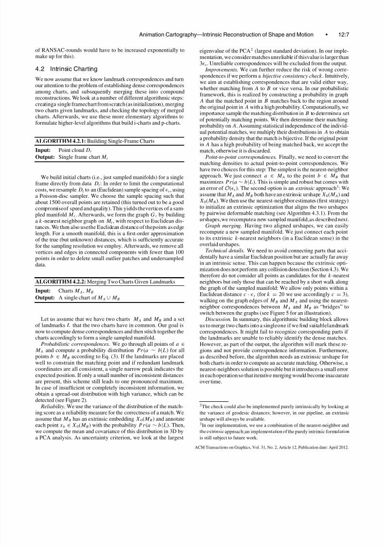
Technical details. We need to avoid connecting parts that acci-dentally have a similar Euclidean position but are actually far awayin an intrinsic sense. This can happen because the extrinsic opti-mization does not perform any collision detection (Section 4.3). Wetherefore do not consider all points as candidates for the k-nearestneighbors but only those that can be reached by a short walk along
the graph of the sampled manifold: We allow only points within aEuclidean distance c · s (for k = 20 we use accordingly c = 3),walking on the graph edges of M B and M A and using the nearest-neighbor correspondences between M A and M B as “bridges” toswitch between the graphs (see Figure 5 for an illustration).
Discussion. In summary, this algorithmic building block allowsus to merge two charts into a singleone if we find suitablelandmark correspondences. It might fail to recognize corresponding parts if the landmarks are unable to reliably identify the dense matches.However, as part of the output, the algorithm will mark these re-gions and not provide correspondence information. Furthermore,as described before, the algorithm needs an extrinsic urshape forboth charts in order to compute an accurate matching. Otherwise, anearest-neighbors solution is possible but it introduces a small errorin each operation so that iterative merging would become inaccurate
over time.
2The check could also be implemented purely intrinsically by looking at
the variance of geodesic distances; however, in our pipeline, an extrinsic
urshape will always be available.3In our implementation, we use a combination of the nearest-neighbor and
the extrinsic approach;an implementation of the purely intrinsic formulation
is still subject to future work.
ACM Transactions on Graphics, Vol. 31, No. 2, Article 12, Publication date: April 2012.
8/12/2019 Animation Cartography - Intrinsic Reconstruction of Shape and Motion
http://slidepdf.com/reader/full/animation-cartography-intrinsic-reconstruction-of-shape-and-motion 8/15
12:8 • A. Tevs et al.
graph A
graph B
topologically incorrectconnection
Fig. 5. Graph merging: The blue and the red graph are merged. Points
within the c · s search range (light green) are potential neighbors of the
center point. We exclude points that are not reachable by walking on the
joint red and blue graph without leaving the search range. Nearest-neighbor
correspondences (green) can be used as “bridges” to walk from blue to red
and back.
ALGORITHM 4.2.3: Resampling a Chart
Input: A chart M .
Output: A resampled version M which is a minimal
s-covering of M
Thenext operationwe need to provide is to reducethe complexityof a chart by resampling. The motivation for this is that we willneed to perform many chart merging operations that will constantlyincrease the sampling density in overlapping parts, which at somepoint becomes a problem in terms of computational costs.
Resampling itself is very easy: We just use the Poisson-discsampler to remove nodes from the graph that are still covered bynearby nodes within a distance of no more than s/2. The remainingchallenge is to maintain the temporal correspondence informationbetween the chart and the actual data. At this point we need toremember that charts encode correspondences by attaching sets of
extrinsic positions of points to which they correspond. Therefore,removing chartpoints deletes valuablecorrespondenceinformation.
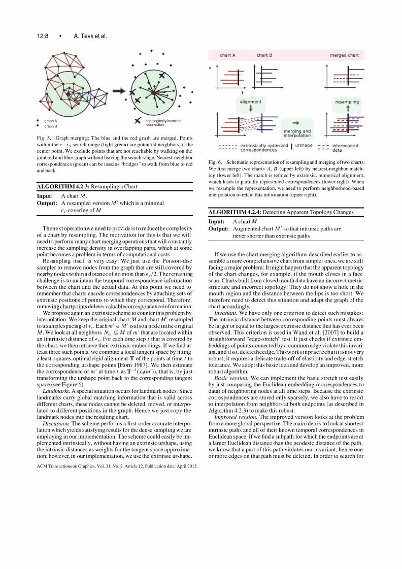
We propose again an extrinsic scheme to counter this problem byinterpolation: We keep the original chartM and chartM resampledto a samplespacing of s . Eachm ∈ M isalsoa node inthe originalM . We look at all neighbors N s ⊆ M of m that are located withinan (intrinsic) distance of s . For each time step t that is covered bythe chart, we then retrieve their extrinsic embeddings. If we find atleast three such points, we compute a local tangent space by fittinga least-squares-optimal rigid alignment T of the points at time t tothe corresponding urshape points [Horn 1987]. We then estimatethe correspondence of m at time t as T−1(x0(m)), that is, by justtransforming the urshape point back to the corresponding tangentspace (see Figure 6).
Landmarks. A special situation occurs for landmark nodes. Since
landmarks carry global matching information that is valid acrossdifferent charts, these nodes cannot be deleted, moved, or interpo-lated to different positions in the graph. Hence we just copy thelandmark nodes into the resulting chart.
Discussion. The scheme performs a first-order accurate interpo-lation which yields satisfying results for the dense sampling we areemploying in our implementation. The scheme could easily be im-plemented intrinsically, without having an extrinsic urshape, usingthe intrinsic distances as weights for the tangent space approxima-tion; however, in our implementation, we use the extrinsic urshape.
Fig. 6. Schematic representation of resampling and merging of two charts:
We first merge two charts A, B (upper left) by nearest-neighbor match-
ing (lower left). The match is refined by extrinsic, numerical alignment,
which leads to partially represented correspondences (lower right). When
we resample the representation, we need to perform neighborhood-based
interpolation to retain this information (upper right).
ALGORITHM 4.2.4: Detecting Apparent Topology Changes
Input: A chart M
Output: Augmented chart M so that intrinsic paths are
never shorter than extrinsic paths
If we use the chart merging algorithms described earlier to as-semble a more comprehensive chart from simpler ones, we are stillfacing a major problem: It might happen that the apparent topologyof the chart changes, for example, if the mouth closes in a facescan. Charts built from closed mouth data have an incorrect metricstructure and incorrect topology: They do not show a hole in themouth region and the distance between the lips is too short. We
therefore need to detect this situation and adapt the graph of thechart accordingly.
Invariant. We have only one criterion to detect such mistakes:The intrinsic distance between corresponding points must alwaysbe larger or equal to the largest extrinsic distance that has ever beenobserved. This criterion is used in Wand et al. [2007] to build astraightforward “edge-stretch” test: It just checks if extrinsic em-beddings of points connected by a common edge violate this invari-ant,and ifso, deletetheedge. Thisworks inpracticebutit isnot veryrobust; it requires a delicate trade-off of elasticity and edge-stretchtolerance. We adopt this basic idea and develop an improved, morerobust algorithm.
Basic version. We can implement the basic stretch test easilyby just comparing the Euclidean embedding (correspondences todata) of neighboring nodes at all time steps. Because the extrinsic
correspondences are stored only sparsely, we also have to resortto interpolation from neighbors at both endpoints (as described inAlgorithm 4.2.3) to make this robust.
Improved version. The improved version looks at the problemfrom a more global perspective: The main idea is to look at shortestintrinsic paths and all of their known temporal correspondences inEuclidean space. If we find a subpath for which the endpoints are ata larger Euclidean distance than the geodesic distance of the path,we know that a part of this path violates our invariant, hence oneor more edges on that path must be deleted. In order to search for
ACM Transactions on Graphics, Vol. 31, No. 2, Article 12, Publication date: April 2012.
8/12/2019 Animation Cartography - Intrinsic Reconstruction of Shape and Motion
http://slidepdf.com/reader/full/animation-cartography-intrinsic-reconstruction-of-shape-and-motion 9/15
Animation Cartography—Intrinsic Reconstruction of Shape and Motion • 12:9
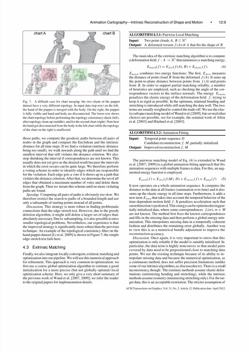
Fig. 7. A difficult case for chart merging: the two charts of the puppet
dataset have a very different topology. In input data (top row) on the left,
the hand of the puppet is merged with the body. On the right, the puppet
is fully visible and hand and body are disconnected. The lower row shows
the chart topology before performing the topology consistency check (left),
after topology clean-up (middle), and for the second chart (right). Note howthe hand got disconnected from the body in the left chart while the topology
of the chart on the right is unaffected.
those paths, we compute the geodesic paths between all pairs of nodes in the graph and compare the Euclidean and the intrinsicdistance for all time steps. If we find a violation (intrinsic distancebeing too small), we walk inwards along the path until we find thesmallest interval that still violates the distance criterion. We alsostop shrinking the interval if correspondences are not known. Thisusually does not yet give us the desired result because the intervalsin which the error occurs can be quite large. We therefore performa voting scheme in order to identify edges which are responsiblefor the violation. Each edge gets a vote if it shows up in a path thatviolates the distance criterion. After that, we determine the set of alledges that obtained a maximum number of votes and delete themfrom the graph. Then we iterate this scheme until no more violatingpaths are found.
Speedup. Computing all pairs of paths is obviously too slow. Wetherefore restrict the search to paths of a bounded length and useonly a subsample of starting points instead of all points.
Discussion. This strategy is more robust in finding problematicconnections than the edge-stretch test. However, due to the greedydeletion algorithm, it might still delete a larger set of edges thanabsolutely necessary. Due to subsampling, it is also possible to misssmaller topological problems. Nevertheless, our experience is thatthe improved strategy is significantly more robust than the previoustechnique. An example of the topological consistency filter on thehand puppet dataset [Li et al. 2009] is shown in Figure 7; the simpleedge-stretch test fails here.
4.3 Extrinsic Matching
Finally, we also integrate locally convergent, extrinsic matching andoptimization into our pipeline. We will use this numerical approachfor refinement. This approach is very common in optimization: wefirst use a coarse global optimization algorithm to estimate a goodinitialization for a more precise (but not globally optimal) localoptimization scheme. Here, we only give a very short summary of the previous work of Wand et al. [2007, 2009]; we refer the readerto the original papers for implementation details.
ALGORITHM 4.3.1: Pairwise Local Matching
Input: Two point clouds A, B ⊂ R3
Output: A deformed version f (A) of A that fits the shape of B
The main idea of the extrinsic matching algorithm is to compute
a deformation field f : A →R
3
that minimizes a matching energy.Ematch(f ) = Edist (f (A), B) + Eelastic(f ). (4)
Ematch combines two energy functions: The first, Edist , measuresthe distance of point cloud B from the deformed f (A). It sums upthe point-to-plane distance between points from f (A) and pointsfrom B. In order to support partial matching reliably, a numberof heuristics are employed, such as checking the angle of the cor-respondence vectors to the surface normals. The energy Eelasticpenalizes the elastic energy of the deformation field f , trying tokeep it as-rigid-as possible. In the optimum, minimal bending andstretching is introduced while still matching the data well. The twoterms are usually weighted to control the trade-off. We use the elas-ticsubspacematching model of Wand et al.[2009], but severalotherchoices are possible, see for example, the seminal work of Allen
et al. [2003] and Haehnel et al. [2003].
ALGORITHM 4.3.2: Animation Fitting
Input: Temporal point sequence D
Candidate reconstruction f, M , partially initialized.
Output: Improved reconstruction f, M
The pairwise matching model of Eq. (4) is extended in Wandet al. [2007; 2009] to a global animation fitting approach that fitsanimation sequences with multiple frames to data. For this, an aug-mented energy function is employed.
Eanim(f ) = Edist (f (M ),D) + Eelastic(f ) + Etemp(f ) (5)
It now operates on a whole animation sequence. It computes thedistance to the data at all frames (summation over time) and it alsosums up the elastic energy in all time steps. Furthermore, it adds anew term Etemp that takes into account the temporal behavior of thetime-dependent motion field f . It penalizes acceleration such thatsmoothmotion is preferred. This energycan be optimizedusingpar-tially initialized data, where some correspondences f t (m), m ∈ M
are not known. The method first fixes the known correspondencesand fills in the missing data and then perform a global energy min-imization. This interpolates missing data in a temporally coherentfashion and distributes the remaining error globally. Another wayto view this is as a numerical bundle adjustment to improve thereconstruction accuracy.
Discussion. Once again, it is very important to stress that thisoptimization is only reliable if the model is suitably initialized. In
particular, the data term is highly nonconvex so that model partscovered by data need to be prepositioned close to matching datapoints. We use the existing technique because of its ability to in-terpolate missing data and because the numerical optimization, asa continuous method, does not suffer precision limitations (unlikesome of our intrinsicalgorithms,as discussednext). There is a smallinconsistency, though: The extrinsic methods assume elastic defor-mations (minimizing bending and stretching), while the intrinsicmethods assume isometry (minimizing stretching only). For the tar-get data, this is an acceptable restriction: The stricter assumption of
ACM Transactions on Graphics, Vol. 31, No. 2, Article 12, Publication date: April 2012.
8/12/2019 Animation Cartography - Intrinsic Reconstruction of Shape and Motion
http://slidepdf.com/reader/full/animation-cartography-intrinsic-reconstruction-of-shape-and-motion 10/15
12:10 • A. Tevs et al.
elastic behavior is a reasonable regularizer, as validated extensivelyin previous work [Haehnel et al. 2003; Wand et al. 2007, 2009;Sußmuth et al. 2008; Li et al. 2009]. Nevertheless, the charting al-gorithm itself could alternatively be formulated in a purely intrinsicfashion. We will discuss this briefly in the following.
5. RECONSTRUCTION PIPELINE
We now use the building blocks developed in the previous sectionto setup a complete animation reconstruction pipeline. We dividethe algorithm into three conceptual stages: i-chart building, p-chart merging, and final optimization.
5.1 Building i-Charts
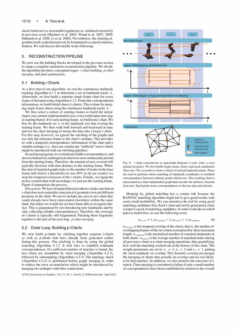
As a first step of our algorithm, we run the continuous landmark tracking Algorithm 4.1.1 to determine a set of landmark tracks L.Afterwards, we first build a separate single frame chart for everyframe of theinput using Algorithm 4.2.1. From this correspondenceinformation, we build initial charts (i-charts). This is done by merg-ing single frame charts using the continuous landmark tracks L.
We first select a subset of starting frames to build the initial
charts (our current implementation uses every tenth input time stepas starting frame). For each starting frame, we build one i-chart. Wefirst fix the landmark set L to the landmark sets that overlap thestarting frame. We then walk both forward and backward in timeand use the chart merging to merge the data into a larger i-chart.For this step, however, we ignore the stitching of the graphs anduse only the reference frame as the chart’s urshape. This providesus with a temporal correspondence information of the chart and asuitable urshape (i.e., does not contain any “artificial” errors whichmight be introduced with our stitching pipeline).
In eachmergingstep, we excludeunreliable correspondences, andalsoexcludenewly startingtracks thatwere not continuously presentfrom the starting frame. Therefore, the amount of area covered willtypically decrease with time distance to the starting frame. Whenthe ratio of matched graph nodes to the number of nodes in the baseframe falls below a threshold (we use 40% in all our results) we
stop the temporal extension of the i-charts. Finally, we equip thenewly created chart with an urshape; we just use the starting frame.Figure 8 summarizes the process.
Discussion. We have designed this procedureto make sure that ani-chart does notcontainthe same pieceof geometry twiceat differentpositions in the chart: We never include any area in an i-chart thatcould already have been represented elsewhere within the samechart, but where we would not yet have been able to recognize thisfact. This is guaranteed by not introducing new landmarks and byonly collecting reliable correspondences. Therefore, the coverageof i-charts is typically still fragmented. Patching these fragmentstogether is the task of the next step, p-chart merging.
5.2 Outer Loop: Building p-Charts
We now build p-charts by stitching together separate i-chartsas well as p-charts that have already been generated earlierduring this process. The stitching is done by using the globalmatching Algorithm 4.1.2. It first tries to establish landmark correspondences. If a sufficient number of matches is found, thetwo charts are assembled by chart merging (Algorithm 4.2.2),followed by subsampling (Algorithms 4.2.3). The topology check (Algorithm 4.2.4) is performed before graph merging in orderto reduce the error accumulation which might be introduced bymerging two urshapes with false connections.
t-1 t t+1
x
t
x
t
per frame charts
space - time diagram, landmark tracks
space - time diagram, charg correspondence established
initial chart
landmark ordinary point
landmark node
ordinary node
chart support
Fig. 8. i-chart construction as spacetime diagram (x-axis: time, y-axis:
spatial location). We first build single frame charts and track landmarks
(first row).The secondrow shows a block of tracked landmark points. These
are used to perform robust matching of landmark coordinates to establish
correspondence between ordinary points (third row). The resulting chart is
represented as a time-independent graph that encodes the intrinsic structure
(last row). Each point stores correspondences to the raw data (not shown).
Merging by global matching has a certain risk because theRANSAC matching algorithm might fail to give good results withsome small probability. We can minimize the risk by using goodmatching candidates first. Each i-chart and newly generated p-chartis kept in a pool of matching candidates. In order to decide on whichpairs to match first, we use the following score.
wscore = λ1woverlap + λ2wmatch + λ3wcommon (6)
woverlap is the temporal overlap of the charts, that is, the number of overlapping frames of the two charts normalized by their maximum
length. wcommon is the normalized number of common landmarks inboth charts. wmatch is the average number of matched nodes duringall previous i-chart or p-chart merging operations, thus quantifyinghow well the matching worked out in the history of this chart. Theweight parameters are set to λ1 = 3, λ2 = 2 and λ3 = 1, puttingthe most emphasis on overlap. This heuristic scoring encouragesthe merging of charts that actually do overlap and are not likelyto be bad matches. In addition, we also monitor the outcome of amatch. Chart merging is considered a failure if only a small numberof correspondences have been established in relation to the overall
ACM Transactions on Graphics, Vol. 31, No. 2, Article 12, Publication date: April 2012.

8/12/2019 Animation Cartography - Intrinsic Reconstruction of Shape and Motion
http://slidepdf.com/reader/full/animation-cartography-intrinsic-reconstruction-of-shape-and-motion 11/15
Animation Cartography—Intrinsic Reconstruction of Shape and Motion • 12:11
number of nodes (in practice, we use 30% as threshold). In caseof failure, the p-chart is not added to the pool and only one of thetwo participating charts is kept. We keep the “better” one judgingby Eq. (6) (omitting the overlap which is not defined for a singlechart).
5.3 Final Optimization
The outer loop described before is run until only one chart is leftin the pool, which is the final reconstructed chart, and the primaryoutput of our method.
We use this chart to drive a final numerical bundle adjustmentaccording to Algorithm 4.3.2. This yields a full motion sequencewhere the urshape of the final chart is deformed to plausibly fit allof the data and move smoothly over time for frames or parts whereno data is available. We show these reconstructions as results inSection 6 and in the accompanying video.
6. RESULTS
We evaluate our algorithm on a number of datasets.First, we use the“Saskia”, “Abhijeet”, and “Kicker” datasets of Vlasic et al. [2009],which have been acquired using a photometric stereo approach. We
also include the “Face” and “Puppet” datasets of Li et al. [2009],which have been acquired with the motion-compensated structuredlight acquisition method of Weise et al. [2007]. Finally, we alsoinclude the “woman”, a dataset that we acquired ourselves using aSwissranger SR4000 [MESA 2012] time-of-flight depth camera. Inaddition to the original datasets we create a shuffled version of the“Face” dataset by deleting subsequences of frames and rearrangingthe remaining data blocks. This dataset is specifically designedto test the performance of our landmark continuation technique,Algorithm 4.1.2. In addition, we also use a synthetic dataset of agesticulating hand, created in Poser 7, to separately evaluate thetwomainnew pipeline stages, landmark tracking and robust charting. Tofully appreciate theresults of ourtechnique we recommendto watchthe accompanying video. A brief summary is shown in Figure 12.
6.1 Synthetic TestsWe first examine the two most important algorithmic componentsof our pipeline separately before we test the complete pipeline.Figure 9 shows a hand model in two different poses with anincreasing amount of missing data. With this example, we examinethe benefits of the robust matching model. The green area indicatesthat the variance of the matching distributions indicates a reliablematch. The robust matching model is able to find reliable matchesfor most of the nonhole area and does not create false positives. If we turn off the robustness, the coverage is substantially reduced.
Figure 10 shows a tracking result on a hand sequence that inthe middle undergoes an abrupt motion. This example examinesthe behavior of the landmark tracking algorithms. In our results,the landmark tracks are correctly interrupted at this point and theRANSAC matching is invoked to build new landmark correspon-
dences. Finally, the dense chart merging is used to obtain globallyconsistent dense correspondences.
6.2 Real-World Scanner Data
The different real-world datasets (see Figure 12 and the video)present a number of challenges to our reconstruction pipeline.For the “Saskia” dataset, the legs of the person often appear tobe connected to the skirt, giving evidence for a different topologythan the correct interpretation of the legs being separately moving
Fig. 9. Effect of robust matching: Matching a (synthetic) hand model with
a simulated acquisition hole. The results (a)–(c) use robust matching so that
still large areas are covered with reliable correspondences (green). In thenonrobust result in the lower right (d), significantly more area outside the
hole region cannot be matched. Dataset created in Poser 7.
Fig. 10. Applying landmark tracking to the hand dataset (synthetic). Up-
per row: The blue tracks are obtained by continuous tracking; They end
automatically at the abrupt turn in the middle. Bottom row: The situation
is recognized automatically and the RANSAC algorithm establishes addi-
tional landmark correspondences. The orange lines indicate the final dense
correspondences.
objects. In addition, we have significant amounts of missing data inthe leg region. Another difficulty is presented by the arms movingupwards in the beginning of the sequence. Since the scanner is notable to resolve the gap between the arms and the body, the surface
seems to undergo some significant deformation. Even thoughthis violates our model, our algorithm is able to process the data.Also note how the legs are reconstructed as separate entities; seeFigure 1 (left). This is only possible using the improved versionof Algorithm 4.2.4, which detects topology changes. The basicvariant proposed in earlier work fails to recognize the individualparts.
The main challenge in the “Face” dataset, which has previouslybeen used for template-based animation reconstruction, is presentedby large amounts of missing data, due to the single camera scanner
ACM Transactions on Graphics, Vol. 31, No. 2, Article 12, Publication date: April 2012.
8/12/2019 Animation Cartography - Intrinsic Reconstruction of Shape and Motion
http://slidepdf.com/reader/full/animation-cartography-intrinsic-reconstruction-of-shape-and-motion 12/15
12:12 • A. Tevs et al.
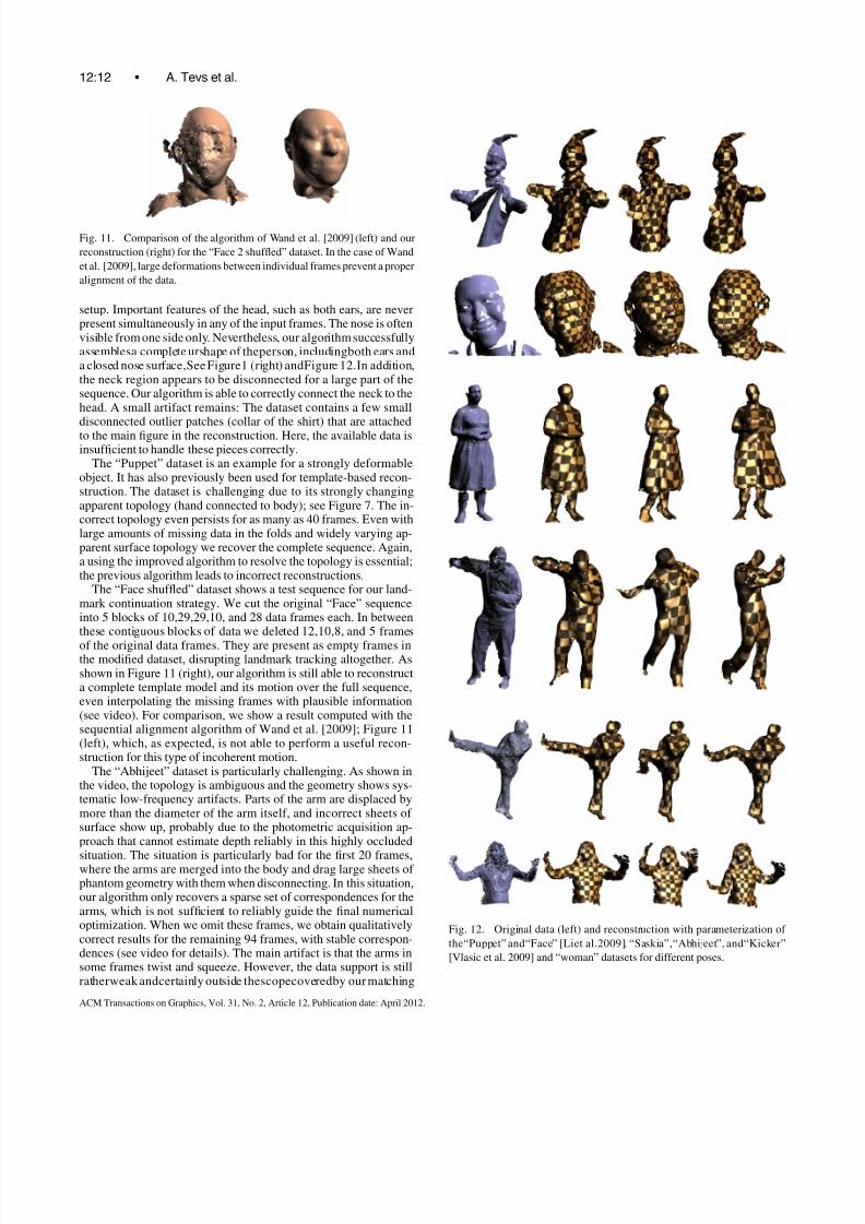
Fig. 11. Comparison of the algorithm of Wand et al. [2009] (left) and our
reconstruction (right) for the “Face 2 shuffled” dataset. In the case of Wand
et al. [2009], large deformations between individual frames prevent a proper
alignment of the data.
setup. Important features of the head, such as both ears, are neverpresent simultaneously in any of the input frames. The nose is oftenvisible from one side only. Nevertheless, our algorithm successfullyassemblesa complete urshape of theperson, includingboth ears anda closed nose surface,See Figure1 (right) andFigure 12.In addition,the neck region appears to be disconnected for a large part of thesequence. Our algorithm is able to correctly connect the neck to thehead. A small artifact remains: The dataset contains a few smalldisconnected outlier patches (collar of the shirt) that are attachedto the main figure in the reconstruction. Here, the available data isinsufficient to handle these pieces correctly.
The “Puppet” dataset is an example for a strongly deformableobject. It has also previously been used for template-based recon-struction. The dataset is challenging due to its strongly changingapparent topology (hand connected to body); see Figure 7. The in-correct topology even persists for as many as 40 frames. Even withlarge amounts of missing data in the folds and widely varying ap-parent surface topology we recover the complete sequence. Again,a using the improved algorithm to resolve the topology is essential;the previous algorithm leads to incorrect reconstructions.
The “Face shuffled” dataset shows a test sequence for our land-mark continuation strategy. We cut the original “Face” sequenceinto 5 blocks of 10,29,29,10, and 28 data frames each. In betweenthese contiguous blocks of data we deleted 12,10,8, and 5 frames
of the original data frames. They are present as empty frames inthe modified dataset, disrupting landmark tracking altogether. Asshown in Figure 11 (right), our algorithm is still able to reconstructa complete template model and its motion over the full sequence,even interpolating the missing frames with plausible information(see video). For comparison, we show a result computed with thesequential alignment algorithm of Wand et al. [2009]; Figure 11(left), which, as expected, is not able to perform a useful recon-struction for this type of incoherent motion.
The “Abhijeet” dataset is particularly challenging. As shown inthe video, the topology is ambiguous and the geometry shows sys-tematic low-frequency artifacts. Parts of the arm are displaced bymore than the diameter of the arm itself, and incorrect sheets of surface show up, probably due to the photometric acquisition ap-proach that cannot estimate depth reliably in this highly occluded
situation. The situation is particularly bad for the first 20 frames,where the arms are merged into the body and drag large sheets of phantom geometry with them when disconnecting. In this situation,our algorithm only recovers a sparse set of correspondences for thearms, which is not sufficient to reliably guide the final numericaloptimization. When we omit these frames, we obtain qualitativelycorrect results for the remaining 94 frames, with stable correspon-dences (see video for details). The main artifact is that the arms insome frames twist and squeeze. However, the data support is stillratherweak andcertainly outside thescopecoveredby our matching
Fig. 12. Original data (left) and reconstruction with parameterization of
the“Puppet” and“Face” [Liet al.2009]. “Saskia”,“Abhijeet”, and“Kicker”
[Vlasic et al. 2009] and “woman” datasets for different poses.
ACM Transactions on Graphics, Vol. 31, No. 2, Article 12, Publication date: April 2012.
8/12/2019 Animation Cartography - Intrinsic Reconstruction of Shape and Motion
http://slidepdf.com/reader/full/animation-cartography-intrinsic-reconstruction-of-shape-and-motion 13/15
Animation Cartography—Intrinsic Reconstruction of Shape and Motion • 12:13
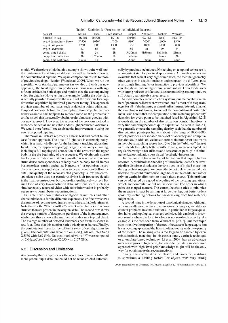
Table I. Statistics for Processing the Individual Datasets
data set Saskia Face Face shuffled Puppet Abhijeet∗ Kicker∗ Woman∗
# frames in seq. 116/116 200/200 141/106 100/100 92/112 20/20 100/100
avg. # data points / frame 20500 10300 10300 9800 20000 16000 8300
avg. # ord. points 1250 1300 1300 1250 1800 2000 3000
avg. # landmarks 82 66 66 86 81 79 34
comp. time i-charts 5h 3h 2h 3h30min 4h30min 1h18min 21min
comp. time outer loop 3h 1h20min 1h 1h40min 1h 19min 2hcomp. time post-proc. 30min 1h 1h 25min 12min 8min 4min
model. We therefore think that this example shows quite well boththe limitations of matching model itself as well as the robustness of the computational pipeline. We again compare our results to thoseof previous local optimization [Wand et al. 2009]. When we run thealgorithm with standard parameters (as we also did with our newapproach), the local algorithm produces inferior results with sig-nificant artifacts in both shape and motion (see the accompanyingvideo for details). However, in this example (unlike the others), itis actually possible to improve the results of the previous local op-timization algorithm by involved parameter tuning: The approachprovides a number of heuristics, such as deleting points with smalltemporal coverage before the final optimization step. In this par-
ticular example, this happens to remove some of the problematicartifacts such that we actually obtain results almost as good as withour new approach. However, the success of the previous method israther coincidental and unstable under slight parameter variations.We would therefore still see a substantial improvement in using thenewly proposed pipeline.
The “woman” dataset represents a stress test and partial failurecase for our approach. The time-of-flight data is extremely noisy,which is a major challenge for the landmark tracking algorithm.In addition, the apparent topology is again constantly changing,including a full topological connection of the arms with the upperbody in the the beginning of the sequence. We obtain only sparsetracking information so that our algorithm was not able to recon-struct dense correspondences reliably over the body for all framesbut some data remains uncharted. Hence,the final optimization pro-
duces a smooth interpolation that in some parts does not follow thedata. The quality of the reconstructed geometry is low; the corre-spondence noise does not permit resolving high-frequency detailsin the final reconstruction, but the result is qualitatively correct. Forsuch kind of very low-resolution data, additional cues such as asimultaneously recorded video with color information is probablynecessary to permit better reconstructions.
In Table I, we show statistics of algorithm runtimes and othercharacteristic data for the different sequences. The first row showsthe number of reconstructed frames versus the available dataframes.Note that for the “Face shuffled” dataset more frames are recon-structed than are present in the original data. The second row showsthe average number of data points per frame of the input sequence,while row three shows the number of nodes in a typical chart.The average number of detected landmarks per frame is shown inrow four. Note that this number varies widely over frames. Finally,the computation times for the different steps of our algorithm aregiven. The computations were run on a 2xQuadCore Intel XeonX5550 with 2.67 GHz. Datasets marked with a “*” were computedon 2xHexaCore Intel Xeon X5650 with 2.67 GHz.
6.3 Discussion and Limitations
As shown by theexamplescenes,the new algorithmis able to handlemore general input data that could not be reconstructed automati-
cally by previous techniques. Not relying on temporal coherence isan important step for practical applications. Although scanners areavailable that scan at very high frame rates, the fact that geometryoften vanishes in acquisition holes and reappears in a different poseis a strongly limiting factor in practice to previous algorithms. Wecan also show that our algorithm is quite robust: Even for datasetswith strong noise or artifacts outside our modeling assumptions, westill obtain qualitatively correct results.
As most complex reconstruction systems, our method has a num-berof parameters.However, wewereableto fix most of theseparam-eters for all of thedatasets, as described in the text. We only adaptedthe sampling resolution s to control the computational costs. The
main issue here is that the computation of the matching probabilitydensities for every point to be matched (used in Algorithm 4.2.2)is quadratic in the number of discretization points. Therefore, avery fine sampling becomes quite expensive. As seen in Table I,we generally choose the sampling density such that the number of discretization points per frame is about in the range of 1000–2000,which provides a reasonable trade-off of accuracy and computa-tionalcosts. In addition,we haveincreased thenumber of landmarksin the robust matching scores from 5 to 6 in the “Abhijeet” datasetas this leads to slightly better results. Finally, we have adapted theregularizer weights for stiffness and acceleration penalty in thefinalnumerical optimization best visual (aesthetic) impression.
Our method still has a number of limitations that require furtherresearch:A problem is the handling of “unreliable” data. Our currentpipeline dismisses this data in the construction of initial i-charts but
during p-chart merging, we currently do not delete uncharted databecause this could reintroduce large holes in the charts, but ratherrely on extrinsic alignment to match these pieces. This problemcan be addressed by a good scheduling of the merging operations,which are commutative but not associative: The order in whichpairs are merged matters. The current heuristic tries to minimizethe negative impact by aiming at large overlap, but better orders(possibly including options for backtracking from bad matches)might exist.
A second issue is the detection of topological changes. Althoughwe can handle more scenes than previous techniques, we still en-counter problems in some situations. In particular, if large acquisi-tion holes and topological changes coincide, this can lead to incor-rect results where the local topology is not resolved correctly. Anexample is the face scan from Wand et al. [2007]. Our techniquecannotresolvethe opening of themouthbecauseof large acquisitionholes opening up around the lips simultaneuously with the openingof the mouth. The missing area is too large to be handled by evenrobust intrinsic matching. In this case, a purely extrinsic techniqueor a template-based technique [Li et al. 2009] has an advantageover our approach. In general, for low-fidelity data, a model-basedapproach with high-level prior knowledge might still be the onlyway for obtaining useful reconstructions.
Finally, the combination of elastic and isometric matchingis sometimes a limiting factor: For objects with very strong
ACM Transactions on Graphics, Vol. 31, No. 2, Article 12, Publication date: April 2012.
8/12/2019 Animation Cartography - Intrinsic Reconstruction of Shape and Motion
http://slidepdf.com/reader/full/animation-cartography-intrinsic-reconstruction-of-shape-and-motion 14/15
12:14 • A. Tevs et al.
deformations, this introduces a bias towards rigidity, leading toinsufficient bending. A purely intrinsic formulation of the chartingcould probably reduce these problems. However, this seems to be aminor issue in practice that can usually be resolved by reducing thestrength of the elastic regularizer appropriately.
7. CONCLUSIONS
We have presented a global optimization technique for animationreconstruction from dynamic point cloud sequences as producedby dynamic range scanning devices. Our method is based on theconcept of cartography and uses an intrinsic framework for a morereliable and robust matching of partial deformable shapes in vastlydifferent poses. Iteratively applying this technique automaticallyyields a completed template model, its motion over the course of the acquired sequence, and a consistent parameterization. Our tech-niqueuses a landmark tracking scheme thatuses temporalcoherenceif available butcan fully automatically resort to an efficientrandom-ized global matching algorithm if required by the data. We can thusrecover from scanner shortcomings such as large-scale occlusionand we can handle fast motion in the scene. We also improve therobustness in detecting topological changes. Overall, we are able toprocess sequences under significantly more general conditions than
previous work.For future work some interesting avenues are opened up by our
research. First,the problem of finding a globally consistent intrinsicdescription of a moving scene can be applied to other problem areas,for example, the computer vision problem of robustly detectingocclusion boundaries in video sequences. Possibly, dynamic scenereconstruction from (multiview) stereo data could be approached bya chartingof consistentparts. Another interesting directionwould beto reformulate the extrinsic matching techniques that we currentlyuse for obtaining subsampling precision in an intrinsic framework.This would make our technique fully isometry invariant. Althoughthis is probably of minor importance in terms of practical results, itwould put the approach in a simpler and more coherent framework.
ACKNOWLEDGMENTSWe would like to thank Leonidas Guibas and Qi-Xing Huang forextensive discussions on intrinsic matching and landmark-basedtechniques. We would also like to thank Vlasic et al. and Li et al. formaking their data available.
REFERENCES
AHMED, N., THEOBALT, C., ROSSL, C., THRUN, S., AND SEIDEL, H.-P. 2008.
Dense correspondence finding for parameterization-free animation re-
construction from video. In Proceedings of the Conference on Computer
Vision and Pattern Recognition (CVPR’08). 1–8.
ALLEN, B., CURLESS, B., AND POPOVIC, Z. 2003. The space of human body
shapes: Reconstruction and parameterization from range scans. ACM
Trans. Graph. 22, 3.
ANGUELOV, D., SRINIVASAN, P., PANG, H.-C., KOLLER, D., THRUN, S., AND
DAVIS, J. 2004. The correlated correspondencealgorithmfor unsupervised
registration of nonrigid surfaces. In Proceedings of the Conference on
Neural Information Processing Systems (NIPS’04).
ANUAR, N. AND GUSKOV, I. 2004. Extracting animated meshes with adaptive
motion estimation. In Proceedings of the Vision, Modeling, and Visual-
ization Workshop (VMV’04). 63–71.
BICKEL, B., BOTSCH, M., ANGST, R., MATUSIK, W., OTADUY, M., PFISTER, H.,
AND GROSS, M. 2007. Multi-Scale capture of facial geometry and motion.
ACM Trans. Graph. 26 , 3, 33.
BRADLEY,D.,HEIDRICH,W.,POPA, T., AND SHEFFER, A.2010. High resolution
passive facial performance capture. ACM Trans. Graph. 29, 41:1-41:10.
BRADLEY, D., POPA, T., SHEFFER, A., HEIDRICH, W., AND BOUFEKEUR, T.
2008. Markerless garment capture. ACM Trans. Graph. 27 , 3, 99.
BRONSTEIN, A. M., BRONSTEIN, M. M., AND KIMMEL, R. 2006. Generalized
multidimensional scaling: A frameworkfor isometry-invariantpartial sur-
face matching. Proc. Nat. Acad. Sci. 103, 5, 1168–1172.
BRONSTEIN, A. M., BRONSTEIN, M. M., AND KIMMEL, R. 2009. Topology-
Invariant similarity of nonrigid shapes. Int. J. Comput. Vis. 81, 3, 281–
301.
BRONSTEIN, A. M., BRONSTEIN, M. M., KIMMEL, R., MAHMOUDI, M., AND
SAPIRO, G. 2010. A gromov-hausdorffframework withdiffusion geometry
for topologically-robust nonrigid shape matching. Int. J. Comput. Vis. 89,
266–286.
CARRANZA, J., THEOBALT, C., MAGNOR, M. A., AND SEIDEL, H.-P. 2003.
Free-Viewpoint video of human actors. ACM Trans. Graph. 22, 569–577.
CHANG, W. AND ZWICKER, M. 2008. Automatic registration for articulated
shapes. Comput. Graph. Forum 27 , 5, 1459–1468.
CHANG, W. AND ZWICKER, M. 2009. Range scan registration using reduced
deformable models. Comput. Graph. Forum 28, 2, 447–456.
CHUM, O. AND MATAS, J. 2005. Matching with PROSAC—Progressive sam-
ple consensus. In Proceedings of the Conference on Computer Vision and Pattern Recognition (CVPR’05). Vol. 1. 220–226.
DAVIS,J. ,NEHAB,D.,RAMAMOORTHI,R., AND RUSINKIEWICZ, S.2005.Space-
time stereo: A unifying framework for depth from triangularization. IEEE
Trans. Pattern Anal. Mach. Intell. 27 , 2, 296–302.
DE AGUIAR, E., STOLL, C., THEOBALT, C., AHMED, N., SEIDEL, H.-P., AND
THRUN, S. 2008. Performance capture fromsparse multi-viewvideo. ACM
Trans. Graph. 27 , 3, 98.
FANG, Q., GAO, J., GUIBAS, L. J., DE SILVA, V., AND ZHANG, L. 2005. Glider:
Gradient landmark-based distributed routing for sensor networks. In Pro-
ceedings of the 24th Conference of the IEEE Communications Society
(InfoCom).
GELFAND, N. AND GUIBAS, L. J. 2004. Shape segmentation using local slip-
page analysis. In Proceedings of the Symposium on Geometry Processing
(SGP’04). 214–223.
HAEHNEL, D., THRUN, S., AND BURGARD, W. 2003. An extension of the
icp algorithm for modeling nonrigid objects with mobile robots. In Pro-
ceedings of the International Joint Conference on Artificial Intelligence
(IJCAI). 915–920.
HORN, B. K. P. 1987. Closed-Form solution of absolute orientation using
unit quaternions. J. Opt. Soc. Amer. A4, 4, 629–642.
HUANG, Q.-X., ADAMS, B., WICKE, M., AND GUIBAS, L. J. 2008. Nonrigid
registration under isometric deformations. Comput. Graph. Forum 27 , 5,
1449–1457.
HUANG, Q.-X., FLORY, S., GELFAND, N., HOFER, M., AND POTTMANN, H.
2006. Reassembling fracturedobjectsby geometricmatching. ACM Trans.
Graph. 25, 3, 569–578.
KONIG, S. AND GUMHOLD, S. 2008. Image-Based motion compensation for
structured light scanning of dynamic scenes. Int. J. Int. Syst. Tech. Appl.
5, 3-4, 434–441.
LEORDENU, M. AND HEBERT, M. 2005. A spectral technique for correspon-
dence problems using pairwise constraints. In Proceedings of the Inter-
national Conference on Computer Vision (ICCV’05). Vol. 2, 1482–1489.
LI, H., ADAMS, B., GUIBAS, L. J., AND PAULY, M. 2009. Robust single-view
geometry and motion reconstruction. ACM Trans. Graph. 28, 5, 175.
LI, H., SUMNER, R. W., AND PAULY, M. 2008. Global correspondence opti-
mization for nonrigid registration of depth scans. Comput. Graph. Forum
27, 5, 1421–1430.
ACM Transactions on Graphics, Vol. 31, No. 2, Article 12, Publication date: April 2012.
8/12/2019 Animation Cartography - Intrinsic Reconstruction of Shape and Motion
http://slidepdf.com/reader/full/animation-cartography-intrinsic-reconstruction-of-shape-and-motion 15/15
Animation Cartography—Intrinsic Reconstruction of Shape and Motion • 12:15
LIAO, M., ZHANG, Q., WANG, H., YANG, R., AND GONG, M. 2009. Modeling
deformable objects from a single depth camera. In Proceedings of the
International Conference on Computer Vision (ICCV’09).
LIPMAN, Y. AND FUNKHOUSER, T. 2009. Mobius voting for surface correspon-
dence. In Proceedings of the SIGGRAPH’09 Conference. ACM Press,
New York, 1–12.
LUCAS,B.D. AND KANADE, T.1981.An iterativeimage registration technique
with an application to stereo vision. In Proceedings of the International Joint Conference on Artificial Intelligence (IJCAI’81). 674–679.
MITRA, N. J., FLORY, S., OVSJANIKOV, M., GELFAND, N., GUIBAS, L., AND
POTTSMANN, H. 2007. Dynamic geometry registration. In Proceedings of
the Symposium on Geometry Processing (SGP’07). 173–182.
OVSJANIKOV, M., MERIGOT, Q., MEMOLI, F., AND GUIBAS, L. 2010. One point
isometricmatchingwith theheat kernel. In Proceedings of the Symposium
on Geometry Processing (SGP’10). 1555–1564.
PARK, S. I. AND HODGINS, J. K. 2006. Capturing and animating skin defor-
mation in human motion. ACM Trans. Graph. 25, 3, 881–889.
PEKELNY, Y. AND GOTSMAN, C. 2008. Articulated object reconstruction and
markerless motion capture from depth video. Comput. Graph. Forum 27 ,
2, 399–408.
POPA, T., SOUTH-DICKENSON, I., BRADLEY, D., SHEFFER, A., AND HEIDRICH,
W. 2010. Globally consistent space-time reconstruction. Comput. Graph.
Forum 29, 5, 1633–1642.SAND, P., MCMILLAN, L., AND POPOVIC, J. 2003. Continuous capture of skin
deformation. ACM Trans. Graph. 22, 3, 578–586.
SHARF,A.,ALCANTARA,D.A.,LEWINER,T.,GREIF,C.,SHEFFER,A.,AMENTA,
N., AND COHEN-OR, D. 2008. Space-Time surface reconstruction using
incompressible flow. ACM Trans. Graph. 27 , 5, 110.
STARCK, J. AND HILTON, A. 2007. Correspondence labeling for wide-
timeframefree-formsurface matching.In Proceedings of the International
Conference on Computer Vision (ICCV’07). 1–8.
SUSSMUTH,J. ,WINTER, M., AND GREINER, G. 2008. Reconstructing animated
meshes from time-varying point clouds. Comput. Graph. Forum 27 , 5,
1469–1476.
TEVS,A.,BERNER,A.,WAND,M.,IHRKE, I., AND SEIDEL, H.-P. 2011. Intrinsic
shape matching by planned landmark sampling. Comput. Graph. Forum
30, 543–552.
TEVS, A., BOKELOH, M., WAND, M., SCHILLING, A., AND SEIDEL, H.-P. 2009.
Isometric registration of ambiguous and partial data. In Proceedings of
the Conference on Computer Vision and Pattern Recognition (CVPR’09).
1185–1192.
VARANASI, K., ZAHARESCU, A., BOYER, E., AND HORAUD, R. P. 2008. Tempo-
ral surface tracking usingmesh evolution. In Proceedings of the European
Conference on Computer Vision (ECCV’08). 30–43.
VLASIC, D., PEERS, P., BARAN, I., DEBEVEC, P., POPOVIC, J., RUSINKIEWICZ,S., AND MATUSIK, W. 2009. Dynamic shape capture using multi-view
photometric stereo. ACM Trans. Graph. 28, 5, 174.
WAND, M., ADAMS, B., OVSJANIKOV, M., BERNER, A., BOKELOH, M., JENKE,
P., GUIBAS, L., SEIDEL, H.-P., AND S CHILLING, A. 2009. Efficient recon-
struction of nonrigid shape and motion from real-time 3D scanner data.
ACM Trans. Graph. 28, 2, 1–15.
WAND, M., JENKE, P., HUANG, Q., BOKELOH, M., GUIBAS, L., AND SCHILLING,
A. 2007. Reconstruction of deforming geometry from time-varying point
clouds. In Proceedings of the Symposium on Geometric Processing
(SGP’07). 49–58.
WEISE, T.,LEIFE,B., AND GOOL, L. V. 2007.Fast 3Dscanningwithautomatic
motion compensation. In Proceedings of the Conference on Computer
Vision and Pattern Recognition (CVPR’07). 1–8.
WURMLIN, S., LAMBORAY, E., STAADT, O. G., AND GROSS, M. H. 2002.
3D video recorder. In Proceedings of the 10th Pacific Conference onComputer Graphics and Applications (PG’02). IEEE Computer Society,
Washington, DC, 325.
ZHANG, L., SNAVELY, N., CURLESS, B., AND SEITZ, S. M. 2004. Space-Time
faces: High resolution capture for modeling and animation. ACM Trans.
Graph. 23, 3, 548–558.
ZHENG, Q., SHARF, A., TAGLIASACCHI, A., CHEN, B., ZHANG, H., SHEFFER,
A., AND COHEN-OR, D. 2010. Consensus skeleton for nonrigid space-time
registration. Comput. Graph. Forum 29, 2, 635–644.
ZITNICK, C. L., KANG, S. B., UYTTENDAELE, M., WINDER, S., AND SZELISKI,
R. 2004. High-Quality video view interpolation using a layered represen-
tation. In ACM SIGGRAPH’04 Papers. ACM, New York, 600–608.
Received February 2011; revised August 2011; accepted October 2011
ACM Transactions on Graphics, Vol. 31, No. 2, Article 12, Publication date: April 2012.