ANGULAR MOMENTUM: AN APPROACH TOCOMBINATORIAL SPACE-TIME

ROGER PENROSE

I want to describe an idea which is related to other things that weresuggested in the colloquium, though my approach will be quite different. Thebasic theme of these suggestions have been to try to get rid of the continuumand build up physical theory from discreteness.

The most obvious place in which the continuum comes into physics is thestructure of space-time. But, apparently independently of this, there is alsoanother place in which the continuum is built into present physical theory.This is in quantum theory, where there is the superposition law: if you havetwo states, you’re supposed to be able to form any linear combination ofthese two states. These are complex linear combinations, so again you havea continuum coming in—namely the two-dimensional complex continuum—in a fundamental way.

My basic idea is to try and build up both space-time and quantum me-chanics simultaneously—from combinatorial principles—but not (at least inthe first instance) to try and change physical theory. In the first place itis a reformulation, though ultimately, perhaps, there will be some changes.Different things will suggest themselves in a reformulated theory, than in theoriginal formulation. One scarcely wants to take every concept in existingtheory and try to make it combinatorial: there are too many things whichlook continuous in existing theory. And to try to eliminate the continuum byapproximating it by some discrete structure would be to change the theory.The idea, instead, is to concentrate only on things which, in fact, are discretein existing theory and try and use them as primary concepts—then to buildup other things using these discrete primary concepts as the basic buildingblocks. Continuous concepts could emerge in a limit, when we take more andmore complicated systems.

The most obvious physical concept that one has to start with, wherequantum mechanics says something is discrete, and which is connected withthe structure of space-time in a very intimate way, is in angular momentum.The idea here, then, is to start with the concept of angular momentum—here one has a discrete spectrum—and use the rules for combining angular

This paper originally appeared in Quantum Theory and Beyond, edited by Ted Bastin,Cambridge University Press 1971, pp. 151–180.

1

momenta together and see if in some sense one can construct the concept ofspace from this.

One of the basic ideas here springs from something which always usedto worry me. Suppose you have an electron or some other spin 1

2h particle.

You ask it about its spin: is it spinning up or down? But how does it knowwhich way is ‘up’ and which way is ‘down’? And you can equally well askthe question whether it spins right or left. But whatever question you askit about directions, the electron has only just two directions to choose from.Whether the alternatives are ‘up’ and ‘down’, or ‘right’ and ‘left’ depends onhow things are connected with the macroscopic world.

Also you could consider a particle which has zero angular momentum.Quantum mechanics tells us that such a particle has to be spherically sym-metrical. Therefore there isn’t really any choice of direction that the particlecan make (in its own rest-frame). In effect there is only one ‘direction’. Sothat a thing with zero angular momentum has just one ‘direction’ to choosefrom and with spin one-half it would have two ‘directions’ to choose from.Similarly, with spin one, there would always be just three ‘directions’ tochoose from, etc. Generally , there would be 2s + 1 ‘directions’ available toa spin s object.

Of course I don’t mean to imply that these are just directions in spacein the ordinary sense. I just mean that these are the choices available tothe object as regards its state of spin. That is, however we may choose tointerpret the different possibilities when viewed on a macroscopic scale, theobject itself is ‘aware’ only that these are the different possibilities that areopen to it. Thus, if the object is in an s-state, there is but one possibilityopen to it. If it is in a p-state there are three possibilities, etc., etc. I don’tmean that these possibilities are things that from a macroscopic point ofview we would necessarily think of as directions in all cases. The s-state isan example of a case where we would not!

So we oughtn’t at the outset to have the concept of macroscopic space-direction built into the theory. Instead, we ought to work with just thesediscrete alternatives open to particles or to simple systems. Since we don’twant to think of these alternatives as referring to pre-existing directions ofa background space—that would be to beg the question—we must deal onlywith total angular momentum (j-value) rather than spin in a direction (m-value).

Thus, the primary concept here has to be the concept of total angularmomentum not the concept of angular momentum in, say, the z-direction,

2

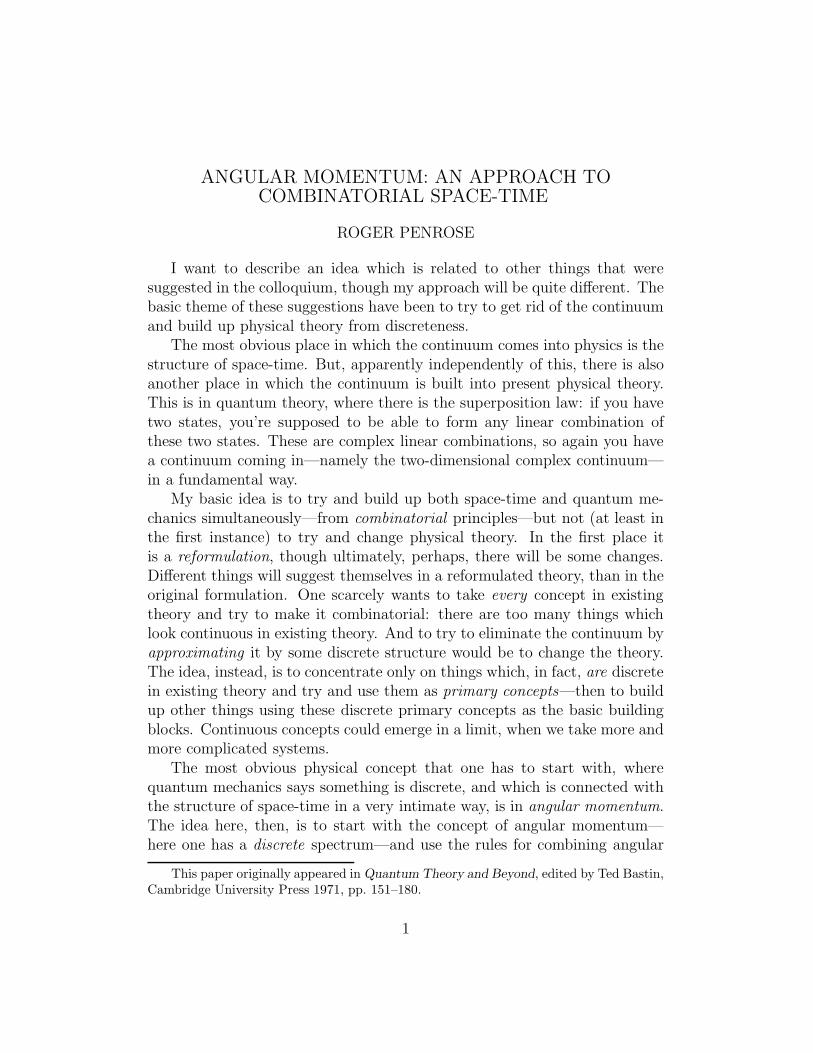
because: which is the z-direction?Imagine, then, a universe built up of things like that shown in fig. 1.

These lines may be thought of as the world-lines of particles. We can viewtime as going in one direction, say, from the bottom of the diagram to thetop. But it turns out, really, that it’s irrelevant which way time is going. SoI don’t want to worry too much about this.

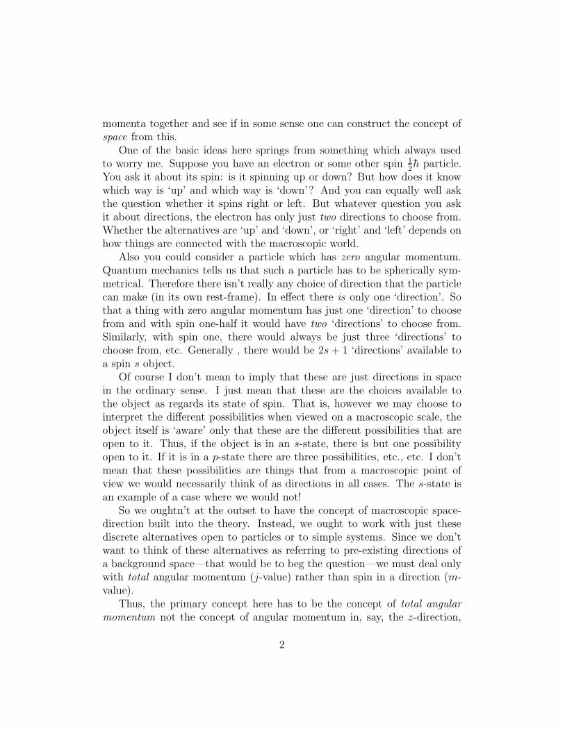
I’m going to put a number on each line. This number, the spin-number

Fig. 1

will have to be an integer. It will represent twice the angular momentum, inunits of h. All the information I’m allowed to know about this picture willbe just this diagram (fig. 2): the network of connections and spin numbers3, 2, 3, . . . like that. I should say

Fig. 2

3

that the picture I want to give here is just a model. Although it does describea type of idealized situation exactly according to quantum theory, I certainlydon’t want to suggest that the universe ‘is’ this picture or anything like that.But it is not unlikely that some essential features of the model that I amdescribing could still have relevance in a more complete theory applicable tomore realistic situations.

I have referred to these line segments as representing, in some way, theworld-lines of particles. But I don’t want to imply that these lines stand justfor elementary particles (say). Each line could represent some compoundsystem which separates itself from other such systems for long enough that(in some sense) it can be regarded as isolated and stationary, with a well-defined total angular momentum n× 1

2h. Let us call such a system or particle

an n-unit. (We allow n = 0, 1, 2, . . .) For the precise model I am describing,we must also imagine that the particles or systems are not moving relativeto one another. They just transfer angular momentum around, regroupingthemselves into different subsystems, perhaps annihilating one another, per-haps producing new units. In the diagram (fig. 2), the 3-unit at the bottomon the left splits into a 2-unit and another 3-unit. This second 3-unit com-bines with a 1-unit (produced in the break up of a 2-unit into two 1-units) tomake a new 2-unit, etc., etc. It is only the topological relationship betweenthe different segments, together with the spin-number values, which is tohave significance. The time-ordering of events will actually play no role here(except conceptually). We could, for example, read the diagram as thoughtime increased from the left to the right, rather than from the bottom to thetop, say.

Angular momentum conservation will be involved when I finally give therules for these diagrams. These rules, though combinatorial, are actuallyderived from the standard quantum mechanics for angular momentum. Thus,in particular, the conservation of total angular momentum must be built intothe rules.

Now, I want to indicate answers to two questions. First, what are thesecombinatorial rules and how are we to interpret them? Secondly, how doesthis enable us to build up a concept of space out of total angular momentum?In order not to get bogged down at this stage with too much detail, I shalldefer, until later on, the complete definition of the combinatorial rules thatwill be used. All I shall say at this stage is that every diagram, such as fig. 2(called a spin-network) will be assigned a non-negative integer which I callits norm. In some vague way, we are to envisage that the norm of a diagram

4

gives us a measure of the frequency of occurrence of that particular spin-network in the history of the universe. This is not actually quite right—Ishall be more precise later—but it will serve to orient our thinking. We shallbe able to use these norms to calculate the probabilities of various spin valuesoccurring in certain simple ‘experiments’. These probabilities will turn outalways to be rational numbers, arising from the fact that the norm is alwaysan integer. Given any spin-network, its norm can be calculated from it in apurely combinatorial way. I shall give the rule later.

But first let me say something about the answer to the second question.How can I say anything about directions in space, when I only have the non-directional concept of total angular momentum? How do I get ‘m-values’ outof j-values, in other words?

Clearly we can’t do quite this. In order to know what the ‘m-value’of an n-unit is, we would require knowledge of which direction in space isthe ‘z-direction’. But the ‘z-direction’ has no physical meaning. Instead,we may ask for the ‘orientation’ of one of our n-units in relation to somelarger structure belonging to the system under consideration. We need somelarger structure which in fact does give us something that we may regardas a well-defined ‘direction in space’ and which could serve in place of the‘z-direction’. As we have seen, a structure of spin zero, being sphericallysymmetrical, is no good for this; spin 1

2h is not much better; spin h only

a little better; and so on. Clearly we need a system involving a fairly largetotal angular momentum number if we are to obtain a reasonably well-defined‘direction’ against which to test the ‘spin direction’ of the smaller units. Wemay imagine that for a large total angular momentum number N , we havethe potentiality, at least, to define a well-defined direction as the spin axis ofthe system. Thus, if we define a ‘direction’ in space as something associatedwith an N -unit with a large N value (I call this a large unit), then we canask how to define angles between these ‘directions’. And if we can decide ona good way of measuring angles, we can then ask the question whether theangles we get are consistent with an interpretation in terms of directions in aEuclidean three-dimensional space, or perhaps in some other kind of space.

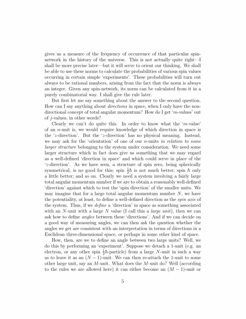
How, then, are we to define an angle between two large units? Well, wedo this by performing an ‘experiment’. Suppose we detach a 1-unit (e.g. anelectron, or any other spin 1

2h-particle) from a large N -unit in such a way

as to leave it as an (N − 1)-unit. We can then re-attach the 1-unit to someother large unit, say an M -unit. What does the M -unit do? Well (accordingto the rules we are allowed here) it can either become an (M − 1)-unit or

5

an (M + 1)-unit. There will be a certain probability of one outcome and acertain probability of the other. Knowing these probability values, we shallhave information as to the angle between the N -unit and the M -unit. Thus,if our two units are to be ‘parallel’, we would expect zero probability for theM − 1 value and certainty for the M + 1 value. If the two units are to be‘anti-parallel’ we would expect exactly the reverse probabilities. If they are‘perpendicular’, then we would expect equal probability values of 1

2, for each

of the two outcomes. Generally, for an angle θ between the directions of thetwo large units we would expect a

Fig. 3

probability 12− 1

2cos θ for the M -unit to be reduced to an (M − 1)-unit and

a probability 12

+ 12

cos θ for it to be increased to an (M + 1)-unit. Let medraw a diagram to represent this experiment (fig. 3). Here κ represents someknown spin-network. By means of a precise (combinatorial) calculationalprocedure—which I shall describe shortly—we can calculate, from knowl-edge of the spin-network κ, the probability of each of the two possible finaloutcomes. Hence, we have a way of getting hold of the concept of Euclideanangle, starting from a purely combinatorial scheme.

As I remarked earlier, these probabilities will always turn out to be ra-tional numbers. You might think, then, that I could only obtain angles withrational cosines in this way. But this would be a somewhat misleading way ofviewing the situation. With a finite spin-network with finite spin-numbers,

6

the angle can never be quite well-enough defined. I can work out numericalvalues for these ‘cosines of angles’ for a finite spin-network, but these ‘angles’would normally not quite agree with the actual angle of Euclidean space untilI go to the limit.

The view that I am expressing here is that rational probabilities are to beregarded as something which can be more primitive than ordinary real num-ber probabilities. I don’t need to call upon the full continuum of probabilityvalues in order to proceed with the theory. A rational probability p = m/nmight be thought of as arising because the universe has to make a choicebetween m alternative possibilities of one kind and n alternative possibilitiesof another—all of which are to be equally probable. Only in the limit, whennumbers go to infinity do we expect to get the full continuum of probabilityvalues.

Fig. 4

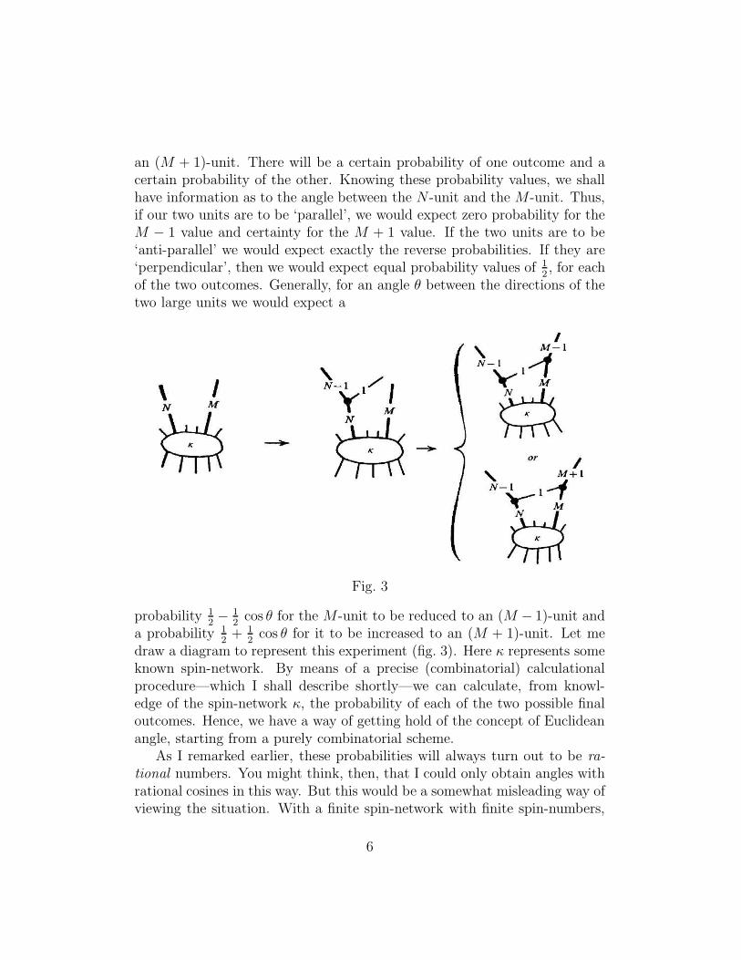
As a matter of fact, it was this question of rational values for primitiveprobabilities arising in nature, which really started me off on this entireline of thought concerning spin-networks, etc. The idea was to find somesituation in nature which one might reasonably regard as giving rise to a‘pure probability’, I am not really sure whether it is fair to assume that ‘pureprobabilities’ exist in nature, but by these I mean probabilities (necessarilyquantum mechanical) whose values are determined by nature alone and notin principle influenced by our ignorance of initial conditions, etc. I supposeI might have thought of branching ratios in particle decays as a possibleexample. Instead, I was led to consider a situation of the following type.

Two spin zero particles each decay into pairs of spin 12h particles. Two of

the spin 12h particles then come together, one from each pair, and combine

to form a new particle (fig. 4). What is the spin of this new particle? Well,

7

it must be either zero or h, with respective probabilities 14

and 34

(assumingno orbital components contribute, etc.). Although you can see that thereare objections even here to regarding this as giving a ‘pure probability’,at least the example served as a starting point. (This example was to someextent stimulated by Bohm’s version of the Einstein-Rosen-Podolsky thoughtexperiment, which it somewhat resembles.) The idea, then, is that any ‘pureprobability’ (if such exists) ought to be something arising ultimately out of achoice between equally probable alternatives. All ‘pure probabilities’ oughttherefore, to be rational numbers.

Fig. 5

But let me leave all this aside since it doesn’t affect the rest of the dis-cussion. Actually, I haven’t quite finished my ‘angle measuring experiment’,so let me return to this.

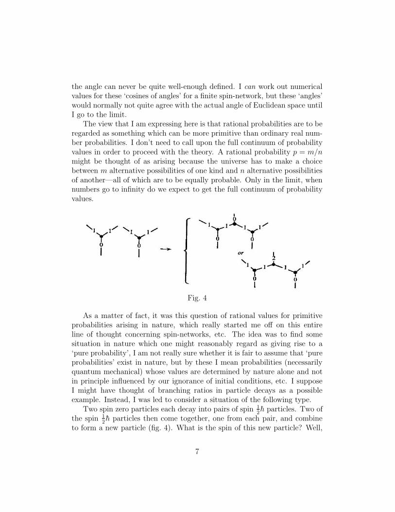
Let us consider the following particular situation. Suppose we have anumber of disconnected systems, each producing a large N -unit. There areto be absolutely no connections between them (fig. 5).

Fig. 6

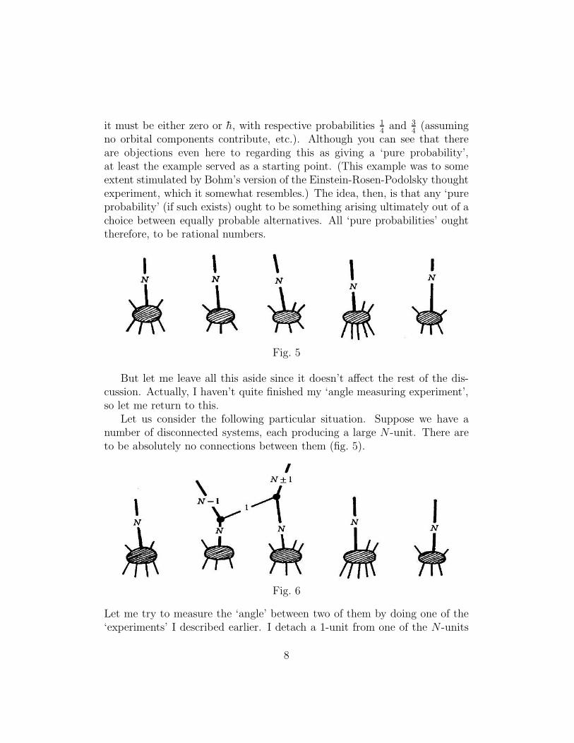
Let me try to measure the ‘angle’ between two of them by doing one of the‘experiments’ I described earlier. I detach a 1-unit from one of the N -units

8

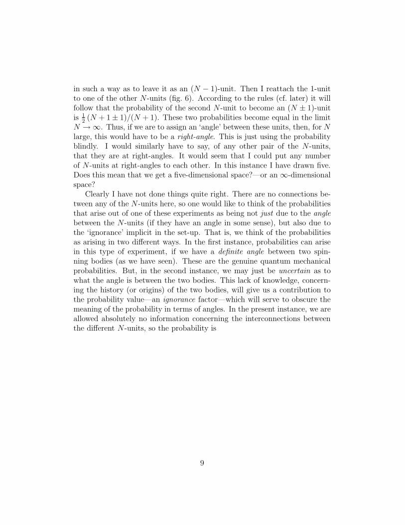
in such a way as to leave it as an (N − 1)-unit. Then I reattach the 1-unitto one of the other N -units (fig. 6). According to the rules (cf. later) it willfollow that the probability of the second N -unit to become an (N ± 1)-unitis 1

2(N + 1± 1)/(N + 1). These two probabilities become equal in the limit

N →∞. Thus, if we are to assign an ‘angle’ between these units, then, for Nlarge, this would have to be a right-angle. This is just using the probabilityblindly. I would similarly have to say, of any other pair of the N -units,that they are at right-angles. It would seem that I could put any numberof N -units at right-angles to each other. In this instance I have drawn five.Does this mean that we get a five-dimensional space?—or an∞-dimensionalspace?

Clearly I have not done things quite right. There are no connections be-tween any of the N -units here, so one would like to think of the probabilitiesthat arise out of one of these experiments as being not just due to the anglebetween the N -units (if they have an angle in some sense), but also due tothe ‘ignorance’ implicit in the set-up. That is, we think of the probabilitiesas arising in two different ways. In the first instance, probabilities can arisein this type of experiment, if we have a definite angle between two spin-ning bodies (as we have seen). These are the genuine quantum mechanicalprobabilities. But, in the second instance, we may just be uncertain as towhat the angle is between the two bodies. This lack of knowledge, concern-ing the history (or origins) of the two bodies, will give us a contribution tothe probability value—an ignorance factor—which will serve to obscure themeaning of the probability in terms of angles. In the present instance, we areallowed absolutely no information concerning the interconnections betweenthe different N -units, so the probability is

9

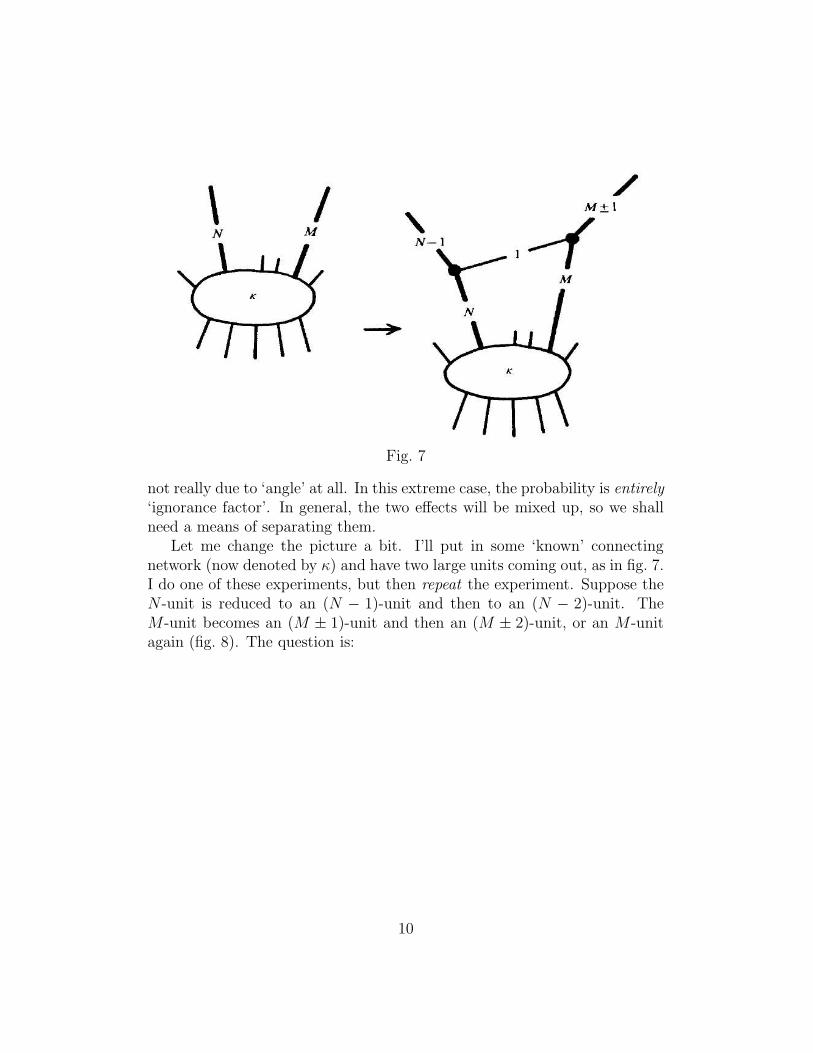
Fig. 7

not really due to ‘angle’ at all. In this extreme case, the probability is entirely‘ignorance factor’. In general, the two effects will be mixed up, so we shallneed a means of separating them.

Let me change the picture a bit. I’ll put in some ‘known’ connectingnetwork (now denoted by κ) and have two large units coming out, as in fig. 7.I do one of these experiments, but then repeat the experiment. Suppose theN -unit is reduced to an (N − 1)-unit and then to an (N − 2)-unit. TheM -unit becomes an (M ± 1)-unit and then an (M ± 2)-unit, or an M -unitagain (fig. 8). The question is:

10

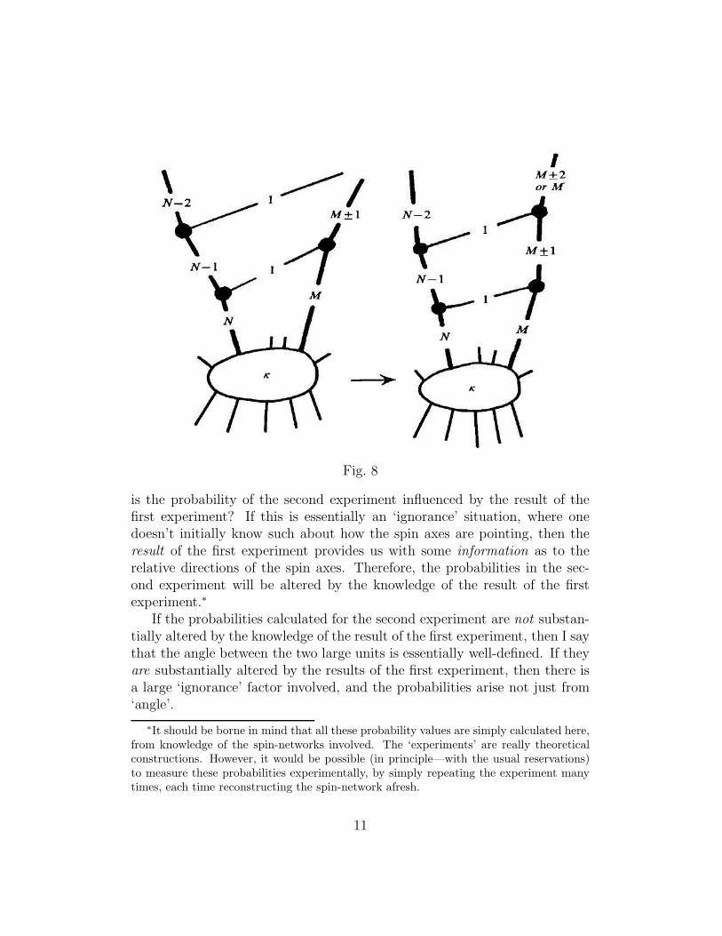
Fig. 8

is the probability of the second experiment influenced by the result of thefirst experiment? If this is essentially an ‘ignorance’ situation, where onedoesn’t initially know such about how the spin axes are pointing, then theresult of the first experiment provides us with some information as to therelative directions of the spin axes. Therefore, the probabilities in the sec-ond experiment will be altered by the knowledge of the result of the firstexperiment.∗

If the probabilities calculated for the second experiment are not substan-tially altered by the knowledge of the result of the first experiment, then I saythat the angle between the two large units is essentially well-defined. If theyare substantially altered by the results of the first experiment, then there isa large ‘ignorance’ factor involved, and the probabilities arise not just from‘angle’.

∗It should be borne in mind that all these probability values are simply calculated here,from knowledge of the spin-networks involved. The ‘experiments’ are really theoreticalconstructions. However, it would be possible (in principle—with the usual reservations)to measure these probabilities experimentally, by simply repeating the experiment manytimes, each time reconstructing the spin-network afresh.

11

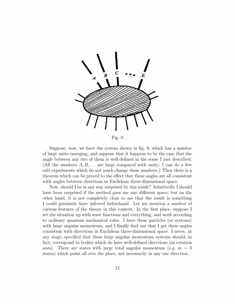
Fig. 9

Suppose, now, we have the system shown in fig. 9, which has a numberof large units emerging, and suppose that it happens to be the case that theangle between any two of them is well-defined in the sense I just described.(All the numbers A,B, . . . are large compared with unity; I can do a fewodd experiments which do not much change these numbers.) Then there is atheorem which can be proved to the effect that these angles are all consistentwith angles between directions in Euclidean three-dimensional space.

Now, should I be in any way surprised by this result? Admittedly I shouldhave been surprised if the method gave me any different space; but on theother hand, it is not completely clear to me that the result is somethingI could genuinely have inferred beforehand. Let me mention a number ofcurious features of the theory in this context. In the first place, suppose Iset the situation up with wave functions and everything, and work accordingto ordinary quantum mechanical rules. I have these particles (or systems)with large angular momentum, and I finally find out that I get these anglesconsistent with directions in Euclidean three-dimensional space. I never, atany stage, specified that these large angular momentum systems should, infact, correspond to bodies which do have well-defined directions (as rotationaxes). There are states with large total angular momentum (e.g. m = 0states) which point all over the place, not necessarily in any one direction.

12

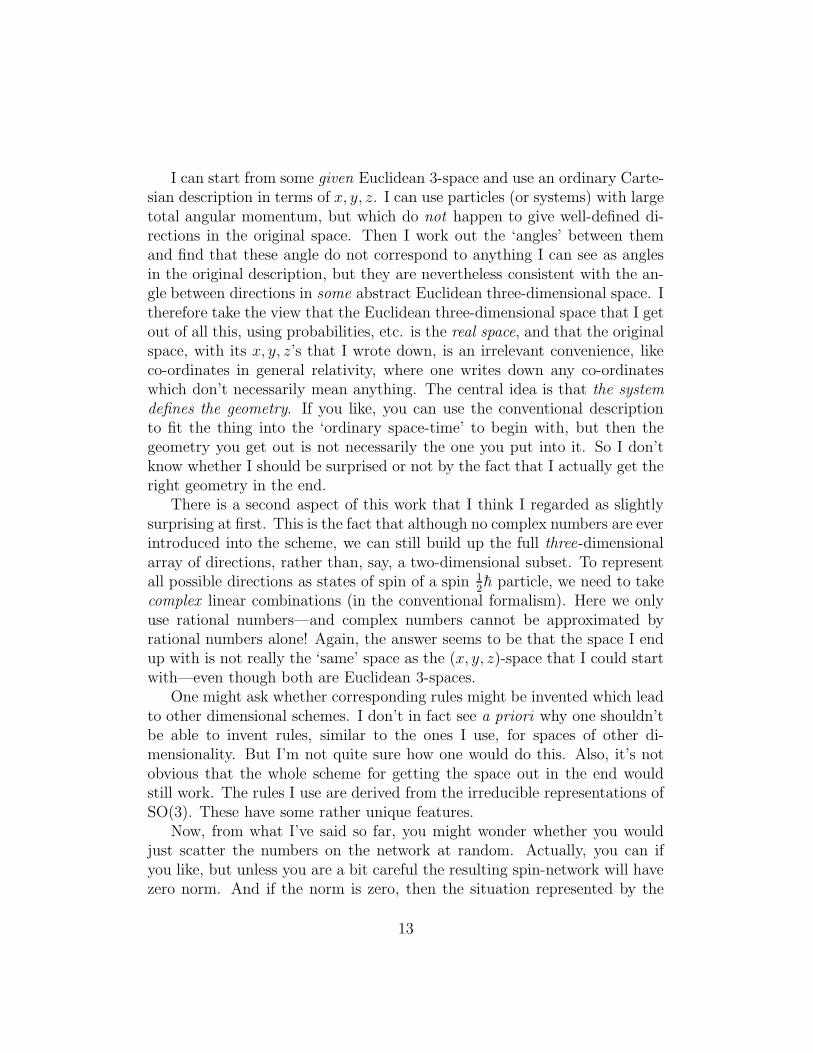
I can start from some given Euclidean 3-space and use an ordinary Carte-sian description in terms of x, y, z. I can use particles (or systems) with largetotal angular momentum, but which do not happen to give well-defined di-rections in the original space. Then I work out the ‘angles’ between themand find that these angle do not correspond to anything I can see as anglesin the original description, but they are nevertheless consistent with the an-gle between directions in some abstract Euclidean three-dimensional space. Itherefore take the view that the Euclidean three-dimensional space that I getout of all this, using probabilities, etc. is the real space, and that the originalspace, with its x, y, z’s that I wrote down, is an irrelevant convenience, likeco-ordinates in general relativity, where one writes down any co-ordinateswhich don’t necessarily mean anything. The central idea is that the systemdefines the geometry. If you like, you can use the conventional descriptionto fit the thing into the ‘ordinary space-time’ to begin with, but then thegeometry you get out is not necessarily the one you put into it. So I don’tknow whether I should be surprised or not by the fact that I actually get theright geometry in the end.

There is a second aspect of this work that I think I regarded as slightlysurprising at first. This is the fact that although no complex numbers are everintroduced into the scheme, we can still build up the full three-dimensionalarray of directions, rather than, say, a two-dimensional subset. To representall possible directions as states of spin of a spin 1

2h particle, we need to take

complex linear combinations (in the conventional formalism). Here we onlyuse rational numbers—and complex numbers cannot be approximated byrational numbers alone! Again, the answer seems to be that the space I endup with is not really the ‘same’ space as the (x, y, z)-space that I could startwith—even though both are Euclidean 3-spaces.

One might ask whether corresponding rules might be invented which leadto other dimensional schemes. I don’t in fact see a priori why one shouldn’tbe able to invent rules, similar to the ones I use, for spaces of other di-mensionality. But I’m not quite sure how one would do this. Also, it’s notobvious that the whole scheme for getting the space out in the end wouldstill work. The rules I use are derived from the irreducible representations ofSO(3). These have some rather unique features.

Now, from what I’ve said so far, you might wonder whether you wouldjust scatter the numbers on the network at random. Actually, you can ifyou like, but unless you are a bit careful the resulting spin-network will havezero norm. And if the norm is zero, then the situation represented by the

13

spin-network a not realizable (i.e. zero probability) according to the rules ofquantum mechanics.

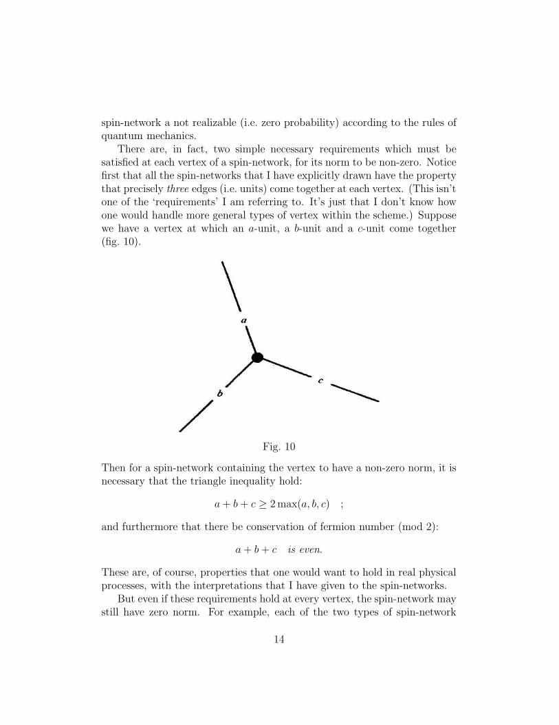
There are, in fact, two simple necessary requirements which must besatisfied at each vertex of a spin-network, for its norm to be non-zero. Noticefirst that all the spin-networks that I have explicitly drawn have the propertythat precisely three edges (i.e. units) come together at each vertex. (This isn’tone of the ‘requirements’ I am referring to. It’s just that I don’t know howone would handle more general types of vertex within the scheme.) Supposewe have a vertex at which an a-unit, a b-unit and a c-unit come together(fig. 10).

Fig. 10

Then for a spin-network containing the vertex to have a non-zero norm, it isnecessary that the triangle inequality hold:

a+ b + c ≥ 2 max(a, b, c) ;

and furthermore that there be conservation of fermion number (mod 2):

a+ b + c is even.

These are, of course, properties that one would want to hold in real physicalprocesses, with the interpretations that I have given to the spin-networks.

But even if these requirements hold at every vertex, the spin-network maystill have zero norm. For example, each of the two types of spin-network

14

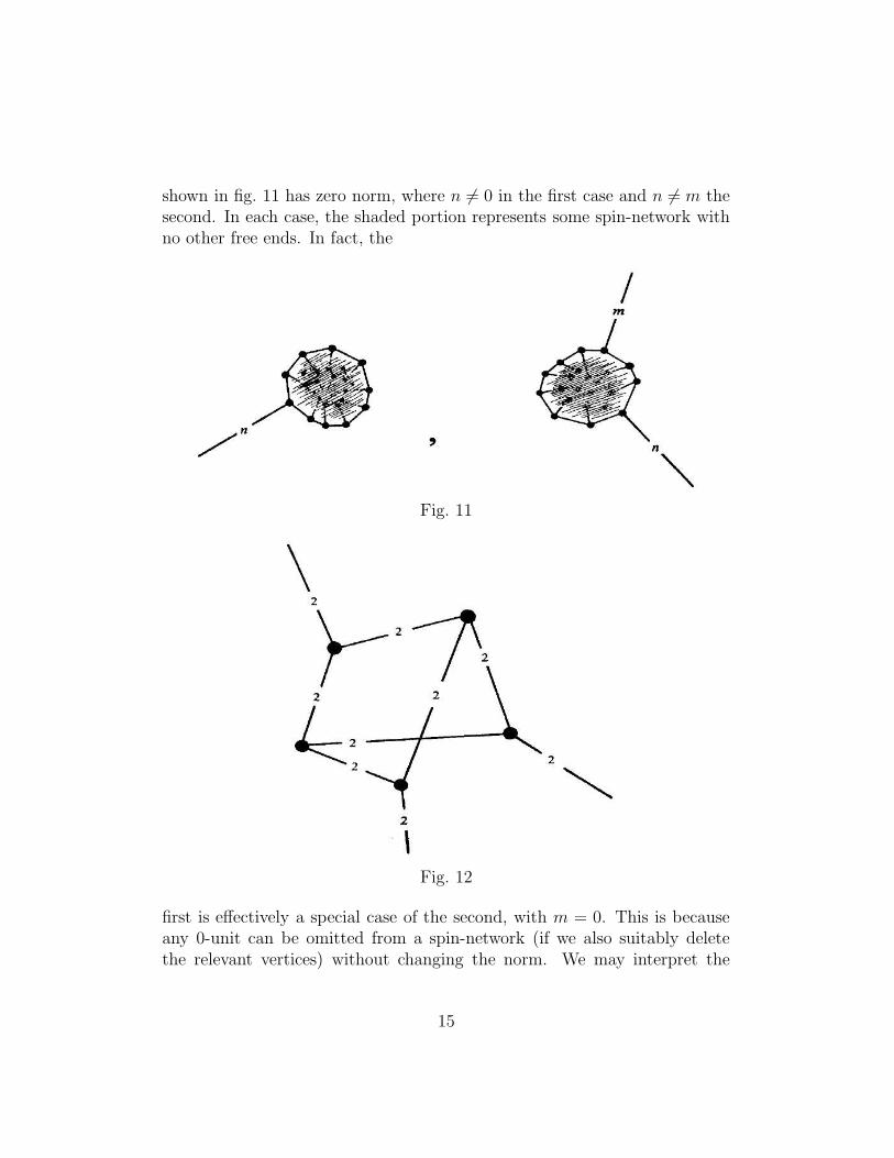
shown in fig. 11 has zero norm, where n 6= 0 in the first case and n 6= m thesecond. In each case, the shaded portion represents some spin-network withno other free ends. In fact, the

Fig. 11

Fig. 12

first is effectively a special case of the second, with m = 0. This is becauseany 0-unit can be omitted from a spin-network (if we also suitably deletethe relevant vertices) without changing the norm. We may interpret the

15

vanishing of the norm whenever n 6= m in the second case as an expressionof conservation of total angular momentum.

In addition to these cases, there are many particular spin-networks whichturn out to have zero norm. One example is shown in fig. 12. But so far Ihave only been giving particular cases. Let us now pass to the general rule.

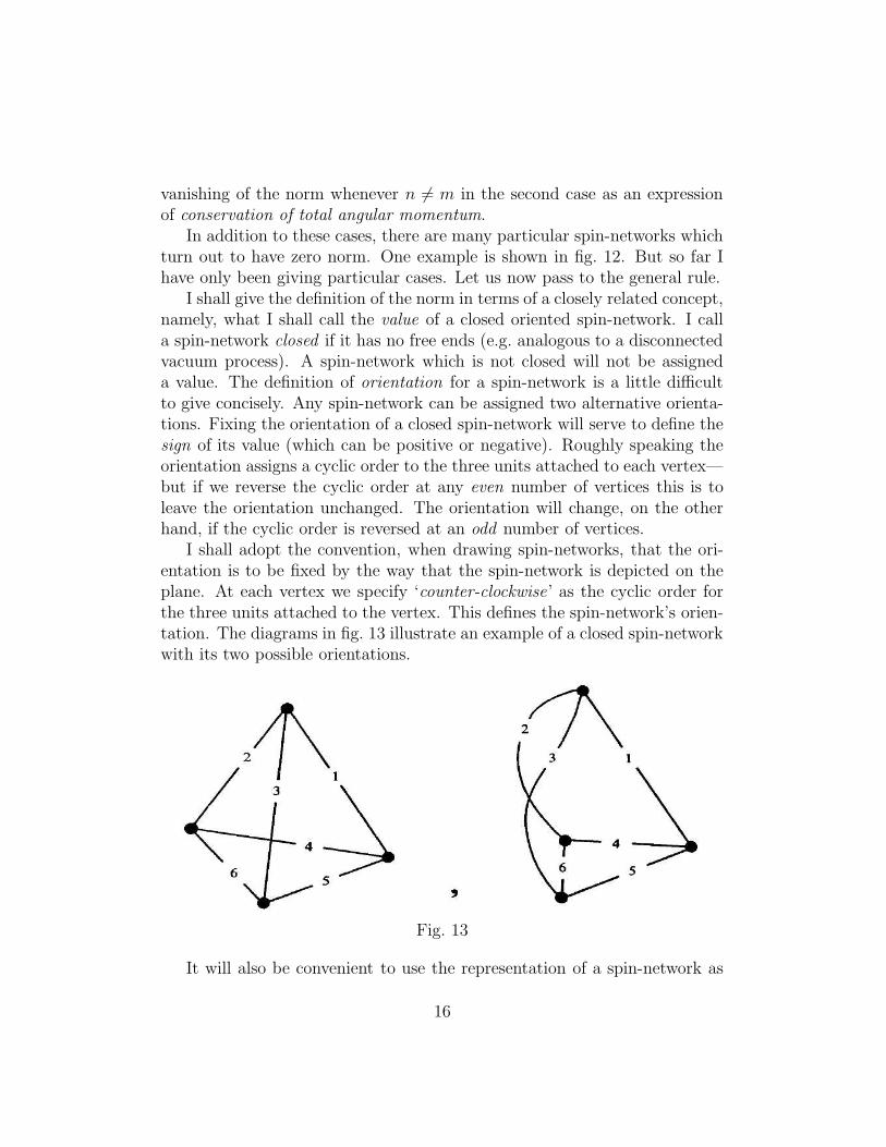
I shall give the definition of the norm in terms of a closely related concept,namely, what I shall call the value of a closed oriented spin-network. I calla spin-network closed if it has no free ends (e.g. analogous to a disconnectedvacuum process). A spin-network which is not closed will not be assigneda value. The definition of orientation for a spin-network is a little difficultto give concisely. Any spin-network can be assigned two alternative orienta-tions. Fixing the orientation of a closed spin-network will serve to define thesign of its value (which can be positive or negative). Roughly speaking theorientation assigns a cyclic order to the three units attached to each vertex—but if we reverse the cyclic order at any even number of vertices this is toleave the orientation unchanged. The orientation will change, on the otherhand, if the cyclic order is reversed at an odd number of vertices.

I shall adopt the convention, when drawing spin-networks, that the ori-entation is to be fixed by the way that the spin-network is depicted on theplane. At each vertex we specify ‘counter-clockwise’ as the cyclic order forthe three units attached to the vertex. This defines the spin-network’s orien-tation. The diagrams in fig. 13 illustrate an example of a closed spin-networkwith its two possible orientations.

Fig. 13

It will also be convenient to use the representation of a spin-network as

16

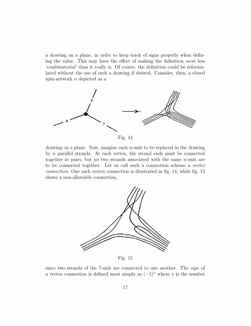
a drawing on a plane, in order to keep track of signs properly when defin-ing the value. This may have the effect of making the definition seem less‘combinatorial’ than it really is. Of course, the definition could be reformu-lated without the use of such a drawing if desired. Consider, then, a closedspin-network α depicted as a

Fig. 14

drawing on a plane. Now, imagine each n-unit to be replaced in the drawingby n parallel strands. At each vertex, the strand ends must be connectedtogether in pairs, but no two strands associated with the same n-unit areto be connected together. Let us call such a connection scheme a vertexconnection. One such vertex connection is illustrated in fig. 14, while fig. 15shows a non-allowable connection,

Fig. 15

since two strands of the 7-unit are connected to one another. The sign ofa vertex connection is defined most simply as (−1)x where x is the number

17

of intersection points between different strands at the vertex, as drawn onthe plane. (These intersection points must be counted correctly if morethan two strands cross at a point, or if two strands touch: and ignored ifa strand crosses itself. It is simplest on the other hand, just to avoid suchfeatures by drawing the strands in general position and not allowing anystrand connection to cross itself.) The sign of a vertex connection, in fact,does not depend on the details of how it is drawn, but only on the pairingoff of the strands. The allowable vertex connection depicted above has −1as its sign, since there are thirteen crossing points.

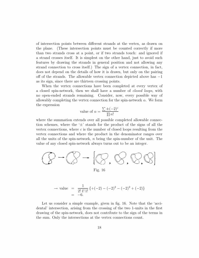
When the vertex connections have been completed at every vertex ofa closed spin-network, then we shall have a number of closed loops, withno open-ended strands remaining. Consider, now, every possible way ofallowably completing the vertex connection for the spin-network α. We formthe expression

value of α =

∑±(−2)c∏n!

where the summation extends over all possible completed allowable connec-tion schemes, where the ‘±’ stands for the product of the signs of all thevertex connections, where c is the number of closed loops resulting from thevertex connections and where the product in the denominator ranges overall the units of the spin-network, n being the spin-number of the unit. Thevalue of any closed spin-network always turns out to be an integer.

Fig. 16

→ value =1

2! 1! 1!{+(−2)− (−2)2 − (−2)2 + (−2)}

= −6.

Let us consider a simple example, given in fig. 16. Note that the ‘acci-dental’ intersection, arising from the crossing of the two 1-units in the firstdrawing of the spin-network, does not contribute to the sign of the terms inthe sum. Only the intersections at the vertex connections count.

18

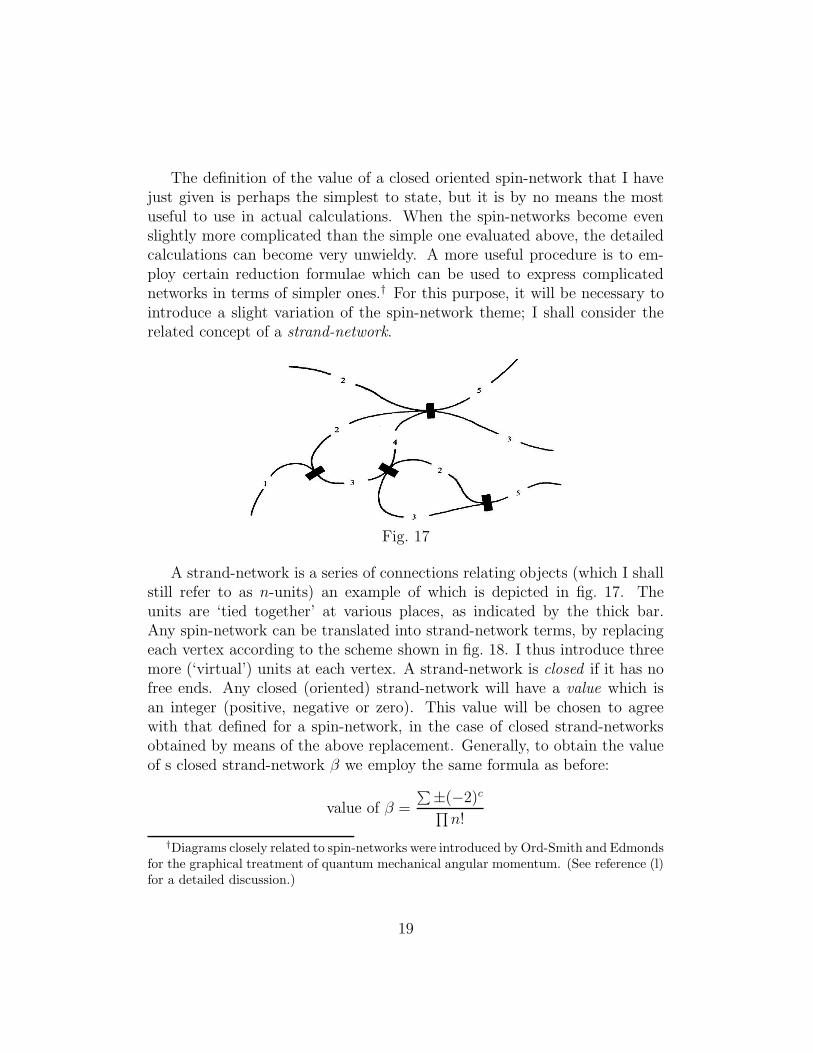
The definition of the value of a closed oriented spin-network that I havejust given is perhaps the simplest to state, but it is by no means the mostuseful to use in actual calculations. When the spin-networks become evenslightly more complicated than the simple one evaluated above, the detailedcalculations can become very unwieldy. A more useful procedure is to em-ploy certain reduction formulae which can be used to express complicatednetworks in terms of simpler ones.† For this purpose, it will be necessary tointroduce a slight variation of the spin-network theme; I shall consider therelated concept of a strand-network.

Fig. 17

A strand-network is a series of connections relating objects (which I shallstill refer to as n-units) an example of which is depicted in fig. 17. Theunits are ‘tied together’ at various places, as indicated by the thick bar.Any spin-network can be translated into strand-network terms, by replacingeach vertex according to the scheme shown in fig. 18. I thus introduce threemore (‘virtual’) units at each vertex. A strand-network is closed if it has nofree ends. Any closed (oriented) strand-network will have a value which isan integer (positive, negative or zero). This value will be chosen to agreewith that defined for a spin-network, in the case of closed strand-networksobtained by means of the above replacement. Generally, to obtain the valueof s closed strand-network β we employ the same formula as before:

value of β =

∑±(−2)c∏n!

†Diagrams closely related to spin-networks were introduced by Ord-Smith and Edmondsfor the graphical treatment of quantum mechanical angular momentum. (See reference (l)for a detailed discussion.)

19

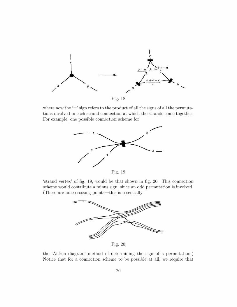
Fig. 18

where now the ‘±’ sign refers to the product of all the signs of all the permuta-tions involved in each strand connection at which the strands come together.For example, one possible connection scheme for

Fig. 19

‘strand vertex’ of fig. 19, would be that shown in fig. 20. This connectionscheme would contribute a minus sign, since an odd permutation is involved.(There are nine crossing points—this is essentially

Fig. 20

the ‘Aitken diagram’ method of determining the sign of a permutation.)Notice that for a connection scheme to be possible at all, we require that

20

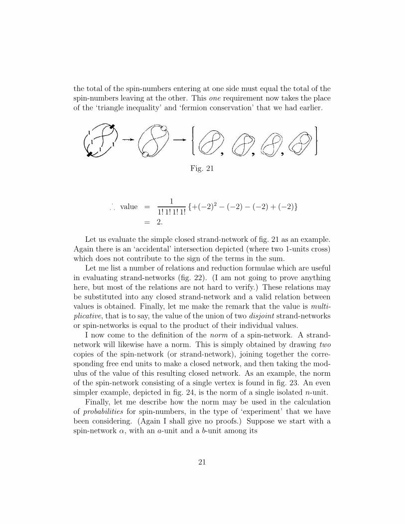
the total of the spin-numbers entering at one side must equal the total of thespin-numbers leaving at the other. This one requirement now takes the placeof the ‘triangle inequality’ and ‘fermion conservation’ that we had earlier.

Fig. 21

·· · value =

1

1! 1! 1! 1!{+(−2)2 − (−2)− (−2) + (−2)}

= 2.

Let us evaluate the simple closed strand-network of fig. 21 as an example.Again there is an ‘accidental’ intersection depicted (where two 1-units cross)which does not contribute to the sign of the terms in the sum.

Let me list a number of relations and reduction formulae which are usefulin evaluating strand-networks (fig. 22). (I am not going to prove anythinghere, but most of the relations are not hard to verify.) These relations maybe substituted into any closed strand-network and a valid relation betweenvalues is obtained. Finally, let me make the remark that the value is multi-plicative, that is to say, the value of the union of two disjoint strand-networksor spin-networks is equal to the product of their individual values.

I now come to the definition of the norm of a spin-network. A strand-network will likewise have a norm. This is simply obtained by drawing twocopies of the spin-network (or strand-network), joining together the corre-sponding free end units to make a closed network, and then taking the mod-ulus of the value of this resulting closed network. As an example, the normof the spin-network consisting of a single vertex is found in fig. 23. An evensimpler example, depicted in fig. 24, is the norm of a single isolated n-unit.

Finally, let me describe how the norm may be used in the calculationof probabilities for spin-numbers, in the type of ‘experiment’ that we havebeen considering. (Again I shall give no proofs.) Suppose we start with aspin-network α, with an a-unit and a b-unit among its

21

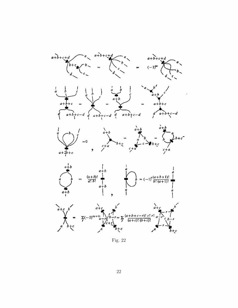
Fig. 22

22

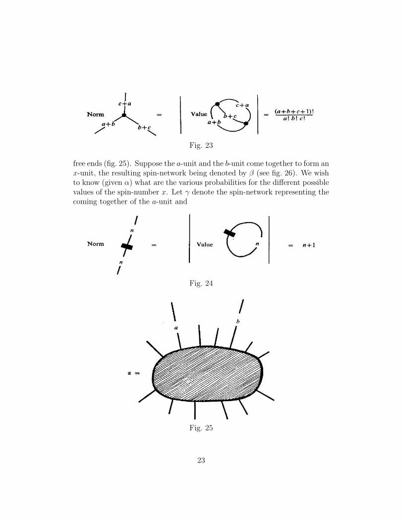
Fig. 23

free ends (fig. 25). Suppose the a-unit and the b-unit come together to form anx-unit, the resulting spin-network being denoted by β (see fig. 26). We wishto know (given α) what are the various probabilities for the different possiblevalues of the spin-number x. Let γ denote the spin-network representing thecoming together of the a-unit and

Fig. 24

Fig. 25

23

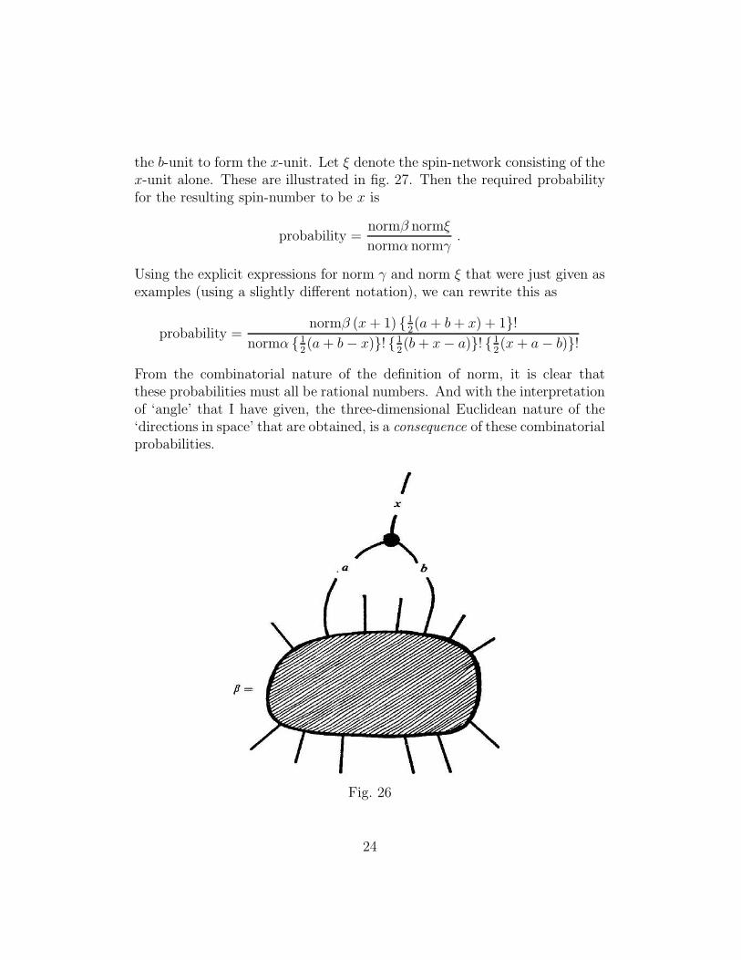
the b-unit to form the x-unit. Let ξ denote the spin-network consisting of thex-unit alone. These are illustrated in fig. 27. Then the required probabilityfor the resulting spin-number to be x is

probability =normβ normξ

normα normγ.

Using the explicit expressions for norm γ and norm ξ that were just given asexamples (using a slightly different notation), we can rewrite this as

probability =normβ (x + 1) { 1

2(a+ b + x) + 1}!

normα {12(a+ b− x)}! { 1

2(b + x− a)}! { 1

2(x+ a− b)}!

From the combinatorial nature of the definition of norm, it is clear thatthese probabilities must all be rational numbers. And with the interpretationof ‘angle’ that I have given, the three-dimensional Euclidean nature of the‘directions in space’ that are obtained, is a consequence of these combinatorialprobabilities.

Fig. 26

24

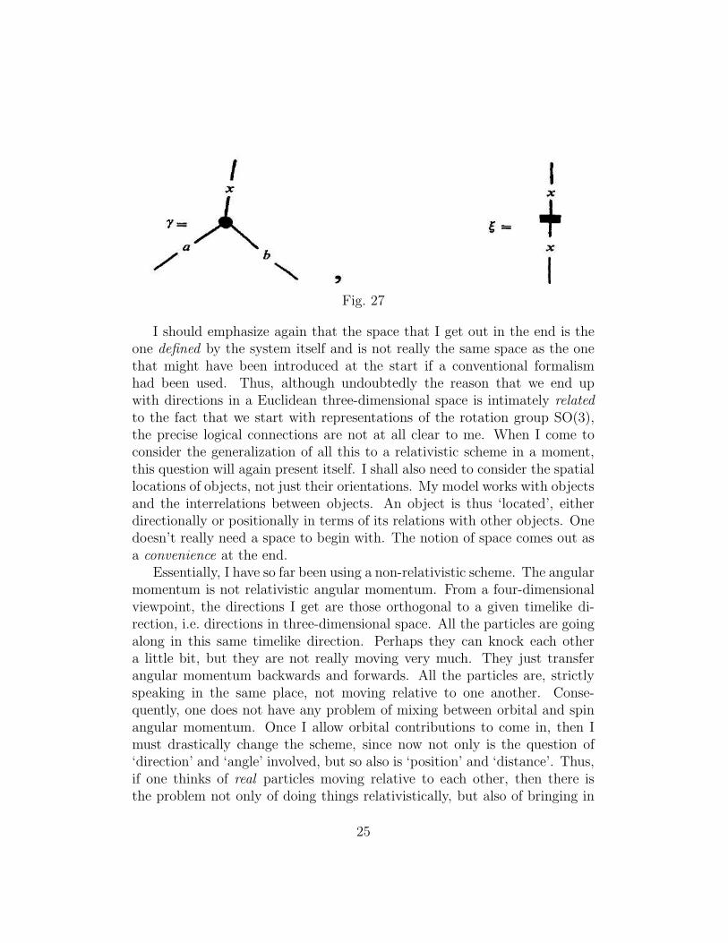
Fig. 27

I should emphasize again that the space that I get out in the end is theone defined by the system itself and is not really the same space as the onethat might have been introduced at the start if a conventional formalismhad been used. Thus, although undoubtedly the reason that we end upwith directions in a Euclidean three-dimensional space is intimately relatedto the fact that we start with representations of the rotation group SO(3),the precise logical connections are not at all clear to me. When I come toconsider the generalization of all this to a relativistic scheme in a moment,this question will again present itself. I shall also need to consider the spatiallocations of objects, not just their orientations. My model works with objectsand the interrelations between objects. An object is thus ‘located’, eitherdirectionally or positionally in terms of its relations with other objects. Onedoesn’t really need a space to begin with. The notion of space comes out asa convenience at the end.

Essentially, I have so far been using a non-relativistic scheme. The angularmomentum is not relativistic angular momentum. From a four-dimensionalviewpoint, the directions I get are those orthogonal to a given timelike di-rection, i.e. directions in three-dimensional space. All the particles are goingalong in this same timelike direction. Perhaps they can knock each othera little bit, but they are not really moving very much. They just transferangular momentum backwards and forwards. All the particles are, strictlyspeaking in the same place, not moving relative to one another. Conse-quently, one does not have any problem of mixing between orbital and spinangular momentum. Once I allow orbital contributions to come in, then Imust drastically change the scheme, since now not only is the question of‘direction’ and ‘angle’ involved, but so also is ‘position’ and ‘distance’. Thus,if one thinks of real particles moving relative to each other, then there isthe problem not only of doing things relativistically, but also of bringing in

25

actual displacements between particles. Consider two particles in relativemotion. Suppose they come together and combine to form a system witha well-defined total spin. Then to obtain the spin of the combined system,we cannot just add up the individual spins because we have to bring in theorbital component. There is a mixture of the actual displacements in spacewith the angular momentum concept. So I spent a long time thinking howone should combine rotations and displacements together into an appropri-ate relativistic scheme. Eventually I was led to consider a certain algebra forspace-time which treats linear displacements on the same footing as it treatsrotations. Thus, linear momentum is treated on a similar footing to angularmomentum.

Now you might raise the objection that linear momentum has a continu-ous spectrum, while it is only for angular momentum that one has discrete-ness. This is a problem of some significance to us. My answer to it is roughlythe following: each particle has its own discrete spectrum for its angular mo-mentum. When two particles are considered together as a unit, then againthere is a discrete spectrum for the combined system. The way these ‘spins’add up implicitly brings in the relative motion between the two particles. Sothe momentum is brought in through the back door, in a sense, for one couldbe always talking in terms of ‘bound systems’.

I consider momentum states as being linear combinations of angular mo-mentum states. There is indeed a problem to see how this continuous mo-mentum should be built up from something discrete, but, in principle, thereis nothing against it. In effect, the idea is that the momentum should bebrought in indirectly. I would propose that, in a sense, there should notbe a well-defined distinction between momentum and angular momentum—except in the limit. Individual particles and simple systems would not really‘know’ what momentum is. Like the idea of ‘direction’ that I consideredearlier, it would be only in the limit of large systems that the concept of mo-mentum really attains a well-defined meaning. Smaller systems might retaina combined concept of momentum and angular momentum, but these thingswould only sort themselves out properly in the limit.

The algebra I have used to treat linear displacements and rotations to-gether, or linear and angular momentum together, I call the algebra oftwistors. I have used the term ‘twistor’ to denote a ‘spinor’ for the six-dimensional (+ + − − −−) pseudo-orthogonal group O(2,4). The twistorgroup is the (+ + −−) pseudo-unitary group SU(2,2), which is locally iso-morphic with O(2,4). In turn, O(2,4) is locally isomorphic with the fifteen-

26

parameter (local) conformal group of space-time. Under a conformal trans-formation of space-time, the twistors will transform (linearly) according to arepresentation of the group SU(2,2).

The basic twistor is a four-complex-dimensional object. We can thusdescribe it by means of four complex components Zα:

(Zα) = (Z0, Z1, Z2, Z3) .

The complex conjugate of the twistor Zα is an object Zα whose components

(Zα) = (Z0, Z1, Z2, Z3)

are given (according to a convenient co-ordinate system) by

Z0 = (Z2), Z1 = (Z3), Z2 = (Z0), Z3 = (Z1).

This implies that the Hermitian form Zα Zα (summation convention as-sumed) has signature (+ + −−), which is required in order to give SU(2,2).(I have already described these objects(2) and their geometrical significancein Minkowski space-time, and a later paper(3) goes into some further devel-opments, including some of the quite surprising aspects of the theory whicharise when one starts to describe physical fields in twistor terms.)

When Zα Zα = 0 I call Zα a null twistor. A null twistor Zα has a verydirect geometrical interpretation in space-time terms. In fact, Zα defines anull straight line, which we can think of as the world line of a zero rest-massparticle. (An important aspect of twistor theory is that zero rest-mass is tobe regarded as more fundamental than a finite rest-mass. Finite mass par-ticles are viewed as composite systems, the mass arising from interactions.)The twistor λZα, for any non-zero complex number λ, defines the same nullline as does Zα. But we can distinguish Zα from λZα by assigning to theparticle a 4-momentum (in its direction of motion) and, in addition, a sortof ‘polarization’ direction (both constant along the world line of the parti-cle). When Zα is replaced by rZα (r real) the momentum is multiplied byr2. When Zα is replaced by eiθZα (θ real) the ‘polarization’ plane is rotatedthrough an angle 2θ. If Y α is another null twistor, the condition for the nulllines represented by Y α and Zα to meet is

Y α Zα = 0,

i.e. this is the condition for the two particles to ‘collide’. (To be strictlyaccurate we have to include the possibility that they may ‘meet at infinity’.

27

In addition, some of the null twistors describe ‘null lines at infinity’ ratherthan actual null lines.)

The non-null twistors are divided into two classes according as Zα Zα,is positive or negative. If Zα Zα > 0, I call Zα right-handed; if Zα Zα < 0,left-handed. In Minkowski space-time, one can give an interpretation of anon-null twistor in terms of a twisting system of null lines. The helicity of thetwist is defined by the sign of Zα Zα. In more physical terms, the twistor Zα

(up the phase) describes the momentum and angular momentum structureof a zero rest-mass particle.‡ We can make the interpretation that Zα Zα,is (twice) the intrinsic spin of the particle, measured in suitable units, witha sign defining the helicity. If Zα Zα 6= 0, then it is not possible actuallyto localize the particle as a null straight line. Only if Zα Zα = 0 do weget a uniquely defined null line which we can think of as the world line ofthe particle; otherwise the particle to some extent spreads itself throughoutspace.

The twistor co-ordinates Z0, Z1, Z2, Z3, together with their complexconjugates Z0, Z1, Z2, Z3, can be used in place of the usual x, y, z, t andtheir canonical conjugates px, py, pz, E. In fact, anything that can be writ-ten in normal Minkowski space terms can be rewritten in terms of twistors.However, in principle, the twistor expressions for even quite simple physicalprocesses may turn out to be very complicated. But in fact it emerges thatthe basic elementary processes that one requires, can actually be expressedvery simply if one goes about it in the right way. Analytic (holomorphic)functions in the Zα variables play a key role. So does contour integration.

We can regard the Zα as quantum operators under suitable circumstances.Then Zα, can be regarded as the canonical conjugate of Zα. (I shall go intothe reasons for this a little more later.) We have commutation rules

Zα Zβ − Zβ Zα = δαβ h

‡Using a convenient co-ordinate system, we can relate the momentum Pα and theangular momentum Mab(= −M ba) to the twistor variables Zα, Zα a by:

P0 + P1 = 212 Z0 Z2, P0 − P1 = 2

12 Z0 Z3, P2 + i P3 = 2

12 Z1 Z2

P2 − i P3 = 212 Z0 Z3, M23 + iM01 = Z1 Z1 − Z0 Z0, M23 − iM01 = Z3 Z3 − Z2 Z2

M13 +M03 + iM02 + iM12 = 2Z2 Z2, M13 −M03 + iM02 − iM12 = 2Z3 Z2

M13 +M03 − iM02 − iM12 = 2Z1 Z0, M13 −M03 − iM02 + iM12 = 2Z0 Z1

28

Then, since Zα and Zα do not commute, we must re-interpret the expressionfor the spin-helicity 1

2n as the symmetrized quantity,

1

4(Zα Zα − Zα Zα) =

1

2nh

Only zero rest-mass states can be eigenstates of this operator. The eigenval-ues of n are . . . − 2,−1, 0, 1, 2, . . . The operators for the ten components ofmomentum and angular momentum (together with those for the five extracomponents arising from the conformal invariance of zero rest-mass fields)are

Zα Zβ −1

4δαβ Z

γ Zγ

in twistor notation. The usual commutation rules for momentum and angularmomentum are then a consequence of the twistor commutation rules.

One idea would now be to use this fact and simply let the twistors takethe place of the two-component spinors that lay ‘behind the scenes’ in myprevious non-relativistic approach, and then to attempt to build a concept ofa four-dimensional space-time from whatever graphical algebra arises fromthe twistor rules. I have not attempted to do quite this, as yet, since I am notsure that it is exactly the right thing to do. There are certain other aspectsof twistor theory which should really be taken into account first.

Let me mention one particular point. It is a rather remarkable one.If the twistor approach is going to have any fundamental significance inphysical theory, then it ought, in principle at least, to be possible to carrythe formalism over and apply it to a curved space-time, rather then just a flatspace-time. These objects, as originally defined, are very much tied up withthe Minkowski flat space-time concept. How can we carry them over into acurved space-time? Actually, a twistor for which Zα Zα = 0 carries over verywell. Its interpretation is now simply as a null geodesic (i.e. world line of afreely moving massless particle) with a momentum (pointing along the worldline) and a ‘polarization’ direction (both covariantly constant along the worldline). On the other hand, it does not seem to be possible to interpret a non-null twistor, in a general curved space-time, in precise classical space-timeterms. Nevertheless it turns out to be convenient to postulate the existenceof these non-null twistors—as objects with no classical realization in curvedspace-time terms. (In a sense, twistors are more appropriate to the treatmentof quantized gravitation§ than of classical general relativity.)

§Since this lecture was delivered, there have been some developments in twistor theory

29

Let us concentrate attention, for the moment, on the null twistors onlyso that we can consider purely geometrical questions. We are interested inproperties of null geodesics which refer to each geodesic as a whole and notto the neighbourhood of some point on a geodesic. Consider, for example,the condition of orthogonality between twistors. We have seen that in flatspace-time, the condition of orthogonality Y αZα = 0 between two twistorsY α, Zα corresponds to the meeting of the corresponding null lines. In curvedspace-time this is not really satisfactory, because although I can tell whethertwo null geodesics are going to meet if I look in the neighbourhood of the in-tersection point, if I look somewhere else, I can’t see whether or not they willmeet, because the curvature may have bent them away from each other. So,in fact, the orthogonality property is not something which is preserved, as aninvariant concept, when one turns to curved space-time. On the other hand,certain things are preserved; and, somewhat surprisingly, they correspond toassigning a symplectic structure to the twistor space.

This symplectic structure is expressed (in appropriate co-ordinates) asthe invariance of the 2-form

dZα ∧ dZα

(using Cartan notation). Strictly speaking, this requires the postulated non-null twistors, in addition to the null ones. The null twistors only forma seven-real-dimensional manifold, whereas a symplectic manifold must beeven-dimensional. The null twistor manifold must be embedded in the eight-real-dimensional manifold consisting of all twistors. The structure of the nulltwistor manifold is that induced by the embedding in this eight-dimensionalsymplectic manifold. In addition to the symplectic structure (and closelyrelated to it), the expressions

ZαZα, ZαdZα, Zα ∂

∂Zα

of relevance to this discussion. It seems to be possible to express quantized gravitationaltheory in twistor form. By means of 3k-dimensional contour integrals in spaces of manytwistor variables, one can apparently calculate scattering amplitudes for processes involv-ing gravitons, photons and other particles. Diagrams arise which can be used to replace thespin-networks of the formalism described here. It is not impossible that the calculationscan be reduced to a set of comparatively simple combinatorial rules, but it is unclear, asyet, whether this is so. The work is still very much at a preliminary stage of developmentand many queries remain unanswered.

30

are also invariant. All these invariant quantities can be interpreted, to someextent, in terms of the geometrical properties of null geodesics. But it willnot be worthwhile for me to go into all this here.

The invariance of the symplectic structure of the twistor space for curvedspace-time can be re-expressed as the invariance of the Poisson brackets

[ψ, χ] = i∂ψ

∂Zα

∂χ

∂Zα− i ∂χ

∂Zα

∂ψ

∂Zα.

This strongly suggests that in the passage to quantum theory, Zα should beregarded as the conjugate variable to Zα. Thus, we are led to the commuta-tion rules I mentioned earlier, relating quantum operators Zα and Zα. Thesecommutation rules in turn give us the commutation relations for momen-tum and angular momentum, as I indicated before. This suggests that theremay possibly be some deep connection between these commutation rules (orperhaps some slight modifications of them) and the curvature of space-time.

The picture that one gets is that in some sense the curvature of space-timeis to do with canonical transformations between the twistor variables Zα, Zα.Suppose we start in some region of space-time where things are essentiallyflat. Then we can interpret Zα and Zα in a straightforward way in termsof geometry and angular momentum, etc. Suppose we then pass through aregion of curvature to another region where things are again essentially flat.We then find that our interpretations have undergone a ‘shift’ correspondingto a canonical transformation between Zα and Zα. In effect the ‘twistorposition’ (i.e. Zα) and ‘twistor momentum’ (i.e. Zα) have got mixed up.Somehow it is this mixing up of the ‘twistor position’ and ‘twistor momentum’which corresponds to what we see as space-time curvature.

Going back to my original combinatorial approach for building space upfrom angular momentum, we can ask now whether such a combinatorialscheme could be applied to the twistors. Might it be that, instead of endingup with a flat space, we could end up with a curved space-time? Even if Istart with the commutation rules appropriate just to the Poincare group, orperhaps the conformal group, it is obvious that I must end up with essentiallythe same space that I ‘start’ with? One has to define the things with whichone builds up geometry (e.g. points, angle, etc.), in terms of the physicalobjects under consideration. It is not at all clear to me that the geometrythat is built up in one region will not be ‘shifted’ with respect to the geometrybuilt up in some other region. Is it then not possible that a space-time

31

possessing curvature might be the result? That is really the final point Iwanted to make.

REFERENCES

(l) Yutsis, A. P., Levinson, I. B. and Vanagas, V. V. Mathematical apparatusof the theory of angular momentum (Jerusalem: I.P.S.T., 1962).(2) Penrose, R. J. Math. Phys. (1967) 8, 345.(3) Penrose, R. Int. Jl Theor. Phys. (1968) 1, 61.

32