Embed Size (px)
Citation preview
Generated using version 3.0 of the official AMS LATEX template
Coupled air–mixed-layer temperature predictability for climate
reconstruction
Angeline G. Pendergrass ∗ Gregory J. Hakim, David S. Battisti
University of Washington, Department of Atmospheric Sciences, Seattle, WA, USA
Gerard Roe
University of Washington, Department of Earth and Space Sciences, Seattle, WA, USA
∗Corresponding author address: Angeline G. Pendergrass, University of Washington, Department of
Atmospheric Sciences, Box 351640, Seattle, WA 98195.
E-mail: [email protected]
1
ABSTRACT
A central issue for understanding past climates involves the use of sparse time-integrated
data to recover the physical properties of the coupled climate system. We explore this issue
in a simple model of the midlatitude climate system that has attributes consistent with
the observed climate. A quasigeostrophic (QG) model thermally coupled to a slab ocean is
used to approximate midlatitude coupled variability, and a variant of the ensemble Kalman
filter is used to assimilate time-averaged observations. Dependence of reconstruction skill on
coupling and thermal inertia are explored. Results from this model are compared with those
for an even simpler two-variable linear stochastic model of midlatitude air–sea interaction,
for which the assimilation problem can be solved semi-analytically.
Results for the QG model show that skill decreases as averaging time increases in both
the atmosphere and ocean when normalized against the time-averaged climatogical variance.
Skill in the ocean increases with slab depth, as expected from thermal-inertia arguments,
but skill in the atmosphere decreases. An explanation of this counterintuitive result derives
from an analytical expression for the forecast error covariance in the two-variable stochastic
model, which shows that the relative fraction of noise to total error increases with slab-ocean
depth. Essentially, noise becomes trapped in the atmosphere by a thermally stiffer ocean,
which dominates the decrease in initial-condition error due to improved skill on the ocean.
Increasing coupling strength in the QG model yields higher skill in the atmosphere and
lower skill in the ocean, as the atmosphere accesses the longer ocean memory and the ocean
accesses more atmospheric high-frequency “noise.” The two-variable stochastic model fails
to cature this effect, showing decreasing skill in both the atmosphere and ocean for increased
coupling strength, due to an increase in the relative fraction of noise to the forecast error vari-
1
ance. Implications for the potential for data assimilation to improve climate reconstructions
are discussed.
1. Introduction
Determining the state of the climate prior to the 20th century necessarily involves pa-
leoclimate proxy data. These data may be viewed as a relatively sparse network of noisy
observations that, in many cases, are indirect records of the climate mediated by biological
or chemical processes. As a result, reconstructions of past climates have relied on statistical
relationships between these proxies and large-scale patterns of atmospheric variability (e.g.,
Mann et al. 1999). One path to potentially improving upon these statistical reconstructions
involves the introduction of a dynamical model to provide independent estimates of the ob-
servations. This approach, which we refer to as dynamical climate reconstruction, links the
paleoclimate reconstruction problem to weather forecasting and modern reanalysis through
the theory of state estimation. Practical realizations of dynamical climate reconstruction
face numerous challenges, only one of which is taken up here. We address the problem of
estimating the state of coupled atmosphere-ocean climate models subject to observations
involving long averaging times typical of paleo-proxy data.
One key issue for dynamical climate reconstruction concerns the predictability time hori-
zon of the model; that is, the time for which initial-condition errors approach the clima-
tological distribution. When the (model) predicted observations are indistinguishable from
a random draw from the climatological distribution, the main value of using the model is
lost. The predictability timescale needed for reconstruction is set by the proxy data, which
2
span a wide range of timescales. “High frequency” paleoclimate records provide information
with at best seasonal, but more typically annual, resolution (e.g., Jones et al. 2009). Since
atmospheric predictability is on the order of two weeks, predictability on the timescales of
these paleoclimate data require dynamics coupled to “slower” parts of the climate system.
For example, sea-surface temperatures have been shown to persist on interannual timescales
in observations (Frankignoul and Hasselmann 1977; Davis 1976, see Deser et al. 2003 for a
modern update) and models (Saravanan et al. 2000). Interest in this persistence has led to
research on variability and predictability in highly idealized models for air-sea interaction
(e.g., Barsugli and Battisti 1998; Saravanan and McWilliams 1998; Scott 2003). On longer
timescales, there is evidence that the overturning circulation in the deep ocean couples to the
atmosphere (e.g., Meehl et al. 2009), which appears responsible for predictable atmospheric
signals beyond the seasonal timescale (Latif 1998; Griffies and Bryan 1997; Grotzner et al.
1999; Boer 2000; Saravanan et al. 2000; Collins 2002; Pohlmann et al. 2004; Latif et al. 2006;
Boer and Lambert 2008; Koenigk and Mikolajewicz 2009).
Paleoclimate proxy data for air temperature and precipitation in midlatitudes represents
climate states integrated over all of the weather during the course of a season or annual cycle.
The characteristics of weather events, and the frequency with which they visit particular
locations, depends on larger-scale, slower varying properties of the atmosphere and ocean.
For example, extratropical cyclones organize in storm tracks, which in turn follow the location
of the jet stream. Thus the reconstruction problem is one where the details of individual
high-frequency features responsible for the proxy data are unknown, but the time average
of these features provides information on slower components of the system.
To address this problem, we use two idealized models of a thermally coupled midlatitude
3
atmosphere and ocean mixed layer that represent both the relevant fast and slow dynamics.
The zero-dimensional energy balance model (referred to hereafter as the BB model) was
designed as an analog to the midlatitude atmosphere-ocean system by Barsugli and Battisti
(1998). The quasigeostrophic (QG) model, developed by Hakim (2000), explicitly calculates
the dominant atmospheric dynamics, and the slab ocean parameters were chosen to corre-
spond to those in the BB model. So, while the models are idealized, they capture important
mechanisms for paleo proxy data.
In order to exploit seasonal or longer predictive timescales and dynamically reconstruct
past climate states, an estimation method is needed to identify accurate initial conditions.
Here we will employ an ensemble Kalman filter (EnKF) technique applied to the above mod-
els of coupled atmosphere–ocean interaction to address two hypotheses: background climate
reconstruction errors become smaller when (1) the thermal heat capacity of the ocean in-
creases, and (2) the coupling between the ocean and atmosphere strengthens. The EnKF
is particularly attractive for addressing these hypotheses because it relaxes the assumption
of stationary statistics made in purely statistical reconstructions. Therefore, information
about the slow component of the system (the ocean) can affect the atmosphere through
both the forecast and the assimilation. Idealized models provide clean control of the pro-
cesses of interest, inexpensive repeatable solutions, and results that can be tested with more
complicated models.
The layout of the paper is as follows. Section 2 introduces the two models and the
assimilation systems built around them. The QG model is described in section 2a, and the
BB model is described in section 2b. Results are given in section 3, with those determined
numerically for the QG model in section 3a and those obtained semi-analytically for the
4
energy-balance model in section 3b. Portions of the error for the energy balance model due
to the initial conditions and accumulation of noise are described in section 3c. Conclusions
are provided in section 4.
2. Method
a. Quasigeostrophic atmosphere model coupled to a slab ocean
To good approximation, the QG equations capture the dynamics of the midlatitude
storm tracks. Moreover, since potential vorticity (PV) is well mixed in the troposphere, the
dynamics may be further approximated by a uniform layer of PV bounded by rigid surfaces
representing the surface and tropopause; this reduces the calculation in three dimensions to
a two-dimensional boundary-value problem (Hakim 2000). This model, when coupled to a
slab ocean model, is referred to hereafter as the QG model.
The atmosphere component of the model is a two-surface dry QG model on an f -plane
that is thermally relaxed to a specified jet (Hoskins and West 1979) on a timescale of 8.6
days. The model is periodic is y and x (latitude and longitude), has an Ekman layer at the
bottom boundary, and solves exactly for the full three-dimensional fields of temperature and
wind given the surface potential temperature. The model was originally described in Hakim
(2000) who provides additional details on the solution methods. An uncoupled version of
the atmosphere model was used by Huntley and Hakim (2009) to explore the time-averaged
data assimilation algorithm for paleoclimate reconstruction proposed by Dirren and Hakim
(2005). Huntley and Hakim (2009) found a predictability horizon beyond which the model no
5
longer provided information distinct from climatology (i.e., a fixed error covariance matrix).
However, this model lacked coupling to components of the climate system that have slower
timescales, which we address here by thermally coupling the QG atmosphere to a slab ocean.
The slab ocean does not move and only exchanges heat with the atmosphere. In order to
preserve the uniform-PV assumption of the atmosphere component of the QG model, heat
is exchanged uniformly at the surface and tropopause (i.e., through the entire depth of the
atmosphere), which is essentially an equivalent barotropic forcing of the atmosphere. The
heat flux is determined by the temperature anomaly difference between the atmosphere’s
surface and the slab ocean, modulated by a coupling constant. More realistic coupling coef-
ficients would also involve the wind speed magnitude or its square, but these were sacrificed
here for simplicity and to provide a link to the analytical model described below. Control
values for the constants in the model are listed in Table 1.
This simple model provides a framework for addressing the two hypotheses in terms of
two parameters: the coupling constant, and the depth of the slab ocean. While this coupled
model provides a testbed to study how the atmosphere, modulated by the slow thermal
inertia of a slab ocean, may be reconstructed on long time scales, it should be clear that this
model does not include nonlinear aspects of heat-flux exchange (e.g., due to wind speed),
ocean dynamics, changes in the mixed layer and its heat capacity, the seasonal cycle, or any
precipitation–evaporation-related processes. However, it does capture the dynamics of heat
exchange between a rapidly evolving atmosphere and a mixed layer with greater thermal
inertia, which is fundamental in midlatitudes. We proceed now to describe the assimilation
system used to reconstruct the model state from noisy observations of time-averages of the
atmosphere and ocean temperature.
6
The EnKF data assimilation system for the QG model is implemented in the Jamaica re-
lease of the Data Assimilation Research Testbed (DART, Anderson et al. 2009), a community-
oriented ensemble data assimilation system. The Ensemble Adjustment Kalman Filter (An-
derson 2001) is used without covariance inflation and with covariance “localization” using
the Gaspari–Cohn function (Gaspari and Cohn 1999) with a half-width of half the domain
to deal with sampling error. Observations are placed at every other grid point, each with
an error of 1/10 of the domain-mean climatological variance for the averaging time of the
observations. Ensembles of 48 members are initialized with random draws of instantaneous
states from a 2500-day integration of the model. Each experiment consists of one ensemble
integration of 100 days without assimilation (the control case) and another integration with
assimilation.
In order to investigate the limit of utility of the reconstruction method, we examine the
background ensemble error variance, which is the error variance at the end of a forecast
cycle immediately before new observations are incorporated in the assimilation cycle. For
comparison, we use an ensemble integrated without assimilating any observations; so the
metric for skill is the error of the background ensemble normalized by the error of the
control ensemble. If this fraction is less than one, then useful information remains from the
previously assimilated observations at assimilation time.
b. Stochastic energy-balance model
A simpler zero-dimensional model of the atmosphere-ocean system provides insights into
the results of the more complex system described above. The model was first introduced by
7
Barsugli and Battisti (1998), and will be referred to hereafter as the BB model. The model
utilizes the large timescale separation in the variance of the atmosphere and ocean to param-
eterize atmospheric nonlinearity as a stochastic process. Stochastic climate models such as
the BB model have a long history of providing a null hypothesis for problems in climate dy-
namics, dating from Hasselmann (1976), who used a stochastic climate model to explore how
persistent, large-scale sea-surface temperature anomalies could arise in midlatitude oceans.
The BB model has thermal exchange between an atmosphere and ocean, damping, and
random forcing applied to the atmosphere:
dTa
dt= c(To − Ta) − τTa + (b − 1)To + N (1)
ddTo
dt= −c(To − Ta) − τTo, (2)
where Ta is the air temperature, To is the mixed layer temperature, d is the ratio of heat
capacities between the atmosphere and mixed layer, c is the coupling strength, τ is the
radiative damping timescale, b is a constant controlling the deterministic portion of the
atmospheric forcing, and N is the white-noise forcing. Equations (1) and (2) can be written
compactly as
d~T
dt= A~T + N ~W, (3)
where
A =
−c − τ c + b − 1
c/d (−c − τ)/d
, N =
N 0
0 0
,
~T = [Ta To] is a vector of the temperatures, and ~W = [W 0] is a Gaussian white-noise
process. The constants b, c, d, τ , and N are chosen to be representative of climate-scale
8
atmosphere-ocean interaction in the midlatitudes (see Table 1 and Barsugli and Battisti
1998).
In the absence of noise forcing, this system supports two normal-mode solutions that are
damped in time, which provide a convenient basis for understanding the system dynamics
with noise. The first mode damps quickly, with an e-folding timescale of 3 days for the
parameters in Table 1, and consists of a mainly atmospheric temperature anomaly with a
weaker ocean temperature anomaly of opposite sign, as noted by Schopf (1985) for a similar
deterministic model. The second mode has a an e-folding timescale of 89 days, and consists of
ocean and atmosphere temperature anomalies of the same sign, with larger magnitude in the
ocean by roughly a factor of two. This second mode contains the “memory” in the system,
which arises because the ocean anomaly is large and of the same sign as the atmosphere, so
that heat exchange is minimized between the two, resulting in a slow decay.
Because the BB model contains only two variables, the data assimilation reconstruction
problem can be solved semi-analytically. Since we are interested in errors, we need only solve
for the error covariance matrix. The expected error covariance over infinite experiments,
derived in the appendix, is:
⟨
ε∗ε∗T⟩
=1
L2
∫ L
0
eAtε∗(0)dt
(∫ L
0
eAtε∗(0)dt
)T
+1
L2
∫ L
0
(∫ L
s
eA(t−s)Ndt
) (∫ L
s
eA(t−s)Ndt
)T
ds, (4)
where ε∗ is the instantaneous error of an ensemble member, ε∗ is the time-averaged error
of an ensemble member, L is the averaging time, A is the matrix of model parameters, and
N is the matrix of noise forcing coefficients. The first term represents the evolution of the
9
initial error covariance, which for this damped system leads to a decay of error covariance.
The second term involves an integral over the noise which gives exponential growth of error
covariance. We will refer to this second effect as the “accumulation” of noise.
3. Results
Before presenting results, we review the hypotheses outlined in section 1. The first is that
errors in climate reconstruction will be smaller when the thermal heat capacity of the ocean
is larger. The crux of this idea is that increasing the thermal heat capacity lengthens the
persistence timescale of anomalies in the ocean, as discussed in section 2b, which increases the
information carried forward by the model to the time of the analysis. The second hypothesis
is that stronger coupling between the atmosphere and ocean should also reduce errors in
climate reconstruction, especially for the atmosphere. Again, since the ocean is the source
of memory, stronger coupling should imprint that memory onto the atmosphere, enhancing
predictability. For the ocean, the role of coupling is less clear. Stronger coupling imparts
more high-frequency atmospheric “noise” into the ocean, reducing predictability, but some
of the ocean’s persistence is imparted to the atmosphere, which may mitigate this effect.
The data assimilation algorithm used here is designed for dealing with paleoclimate proxy
data, which averages or integrates the climate signal over a period of time. Because inter-
preting the effect of different averaging times is not as straightforward as instantaneous
observations, we consider first the role of averaging time on the error. For instantaneous
data assimilation, analysis errors should be inversely proportional to observation frequency,
since, all other things being equal, more frequent observations provide more information
10
about the instantaneous state of the system if the model forecast is well within the pre-
dictability time horizon. For time-averaged data assimilation, the climatological variance
of the states also decreases with averaging time. Therefore, we scale the observation error
with climatological variance for the timescale of the observations to maintain constant error
relative to climatology. We expect that skill will decrease with averaging time.
a. Results for the coupled QG model
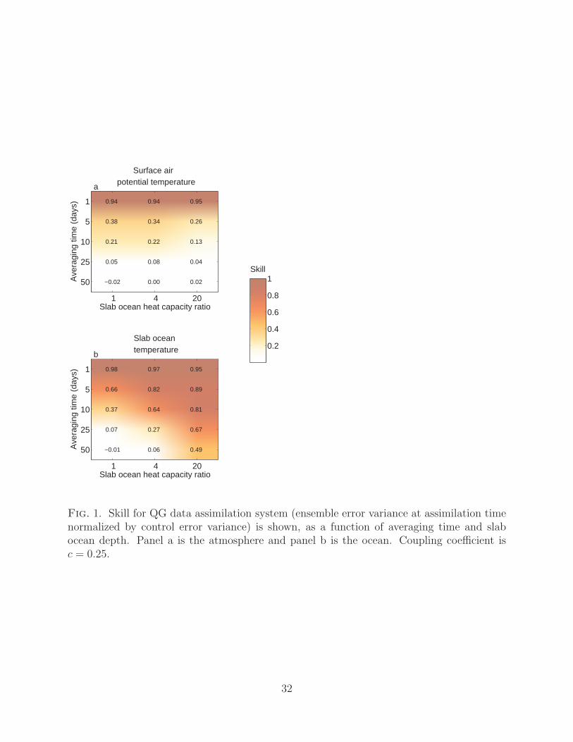
First we consider the dependence of background skill on slab-ocean depth and averaging
time, holding the coupling strength fixed at c = 0.25, shown in Fig. 1. Each pixel is the
skill of the background time-averaged state for a data assimilation experiment of length 100
assimilation cycles, area-averaged over the meridional center of the domain (the region of
basic state meridional temperature gradient). We show skill for the surface temperature
in the atmosphere; skill at the tropopause is nearly identical. The slab ocean depth d is
represented by the ratio of the slab ocean heat capacity to the atmospheric heat capacity.
Results show that for both the atmosphere and ocean, and for all depths of the slab ocean,
skill decreases as the averaging time increases, consistent with prior expectation. There is
a sharp drop of skill between 5 and 10 days, which we suspect corresponds to the model
damping timescale of 8.6 days.
As slab ocean depth increases, skill in the ocean increases, as expected. In contrast,
background skill for the atmosphere decreases with increasing slab-ocean depth, despite the
fact that ocean temperature reconstruction is more skillful. We will revisit these conflicting
results after reviewing those for the BB model.
11
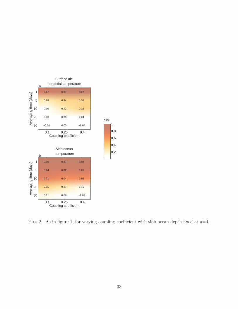
Figure 2 shows the analogous experiment for fixed slab ocean depth ratio at d = 4, and
varying the coupling parameter. For the atmosphere, skill increases slightly with increasing
coupling coefficient. Skill in the ocean decreases as the coupling coefficient gets bigger. These
results are consistent with expectations in the sense that the atmosphere is a source of noise
for the ocean and the ocean is a source of thermal memory for the atmosphere.
In both Figs. 1 and 2 there is a striking difference between skill in the ocean and
atmosphere. This is due to two factors. The first is simply the longer thermal inertia of
the ocean. The process timescales in the ocean are each a factor of d longer than in the
atmosphere, so persistence and predictability in the ocean should be longer. But even for
d=1, when the ocean and atmosphere have the same heat capacity (not shown), the ocean
has longer predictability than the atmosphere. One potential explanation is that since the
ocean has no advection, it integrates over the faster dynamics in the atmosphere, which are
dominated by advection, leading to higher skill at longer time averages.
b. Results for the stochastic energy-balance model
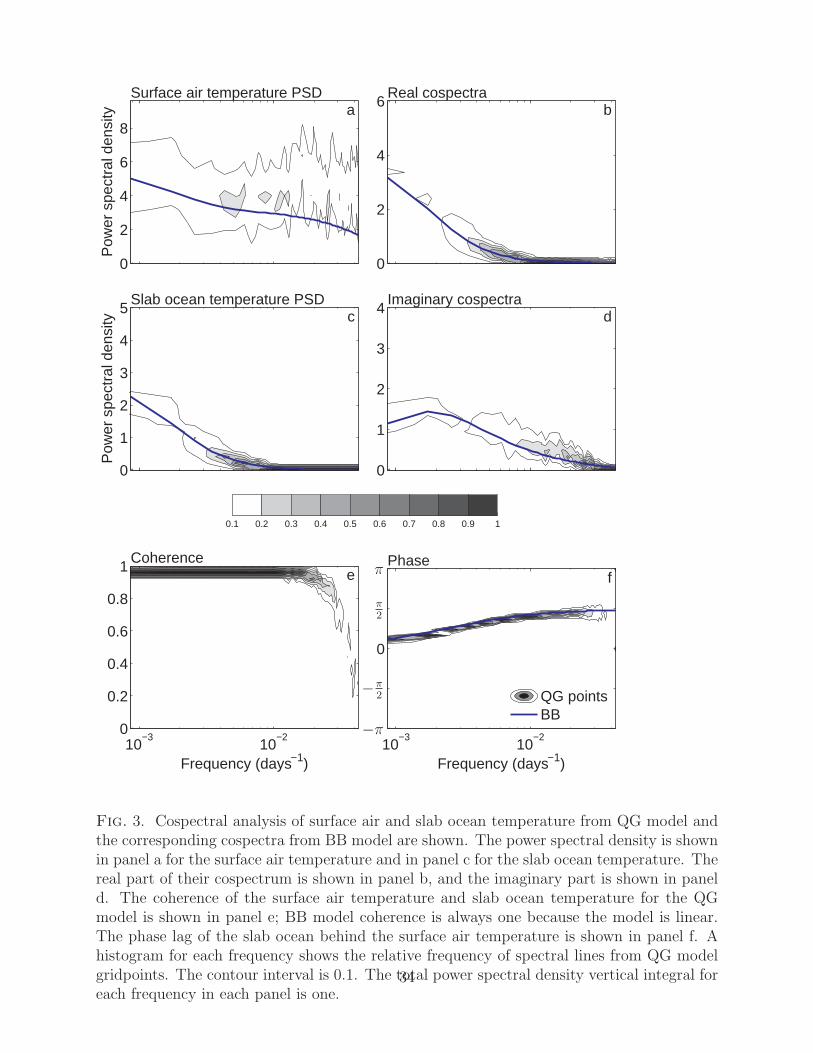
Before reporting the results from the BB model, we will compare its equilibrium statistical
properties with those of the QG model, which it is meant to approximate. Cospectral analysis
of the surface air and slab-ocean temperatures for the QG model are shown in Fig. 3, along
with analytical spectra from the BB model. For the QG model, histograms of analyses are
shown for each grid point in the center half of the domain in the y direction, where the
basic state temperature gradient is nonzero. Analyses apply to the last 8000 days of an 8500
day integration. Ten-day blocks of un-normalized timeseries are averaged together, and then
12
cospectral analysis is carried out with a Hanning window of length 800 days using Matlab’s
spectrum function. Power spectra (Pa and Po), cospectra (Fao), and phase (φ) from the BB
model are calculated from Eqs. (14) and (15) in Barsugli and Battisti (1998),
Pa(σ) =(d2σ2 + (c + τ)2)|N |2
((c + τ)2 − dσ2 − bc) + σ2(1 + d)2(c + τ)2, (5)
Po(σ) =c2|N |2
((c + τ)2 − dσ2 − bc) + σ2(1 + d)2(c + τ)2, (6)
Fao(σ) = TaT∗
o =c|N |2(c + τ + idσ)
((c + τ)2 − dσ2 − bc) + σ2(1 + d)2(c + τ)2, (7)
φ = tan−1 ImFao
ReFao
=dσ
c + τ, (8)
where σ is the frequency, (·)∗ indicates the complex conjugate, and α = bc. Just one line
is shown for the BB model, calculated with parameters b = 0.5 and N = 5, chosen by trial
and error to correspond well the QG model spectra; other parameters are the same as those
for the QG model.
As with the BB model, the spectra of the QG ocean and atmosphere increase toward lower
frequencies; power in the system cannot increase indefinitely because of the damping terms.
The cospectral power increases as frequency decreases in both the BB and QG models, and
there is a low-frequency peak in the quadrature spectrum of both models. The atmosphere
and ocean show high coherence at frequencies below 2π/100 days−1, which then degrades due
to nonlinear effects at high frequencies. The phase relationship of the QG model follows very
closely the BB phase at frequencies for which it is well defined. The close correspondence of
the spectral characteristics of the two models lends confidence that the BB model provides
a good approximation to the QG model for further analysis in a simpler framework.
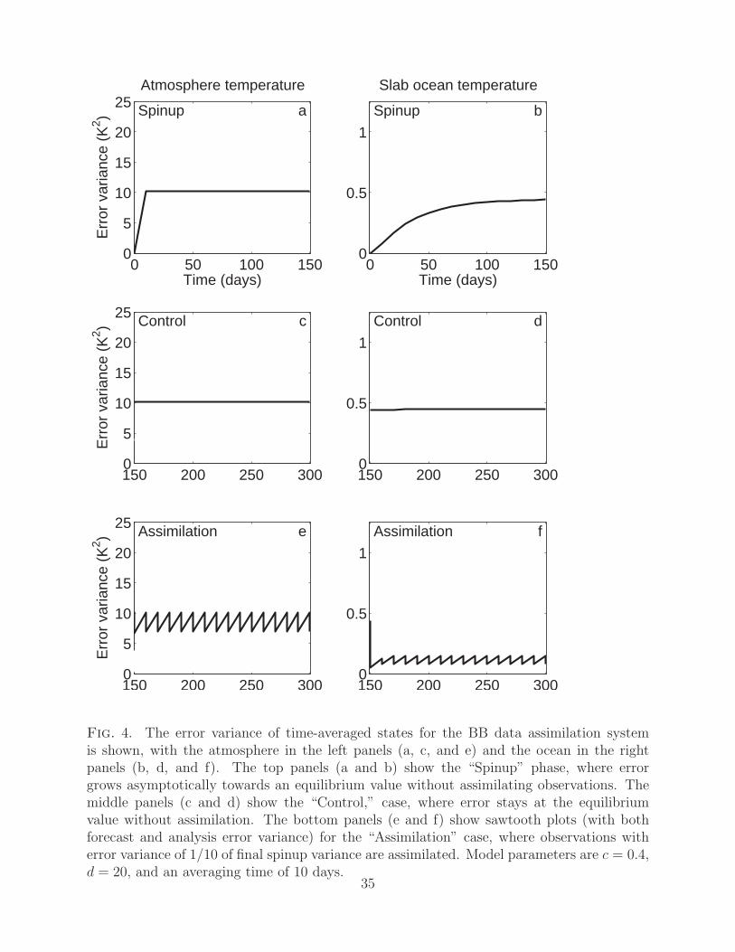
The BB model data assimilation system discussed in section 2b provides the expected
error statistics over an infinite number of experiments and ensemble members. The numerical
13
evaluation of Eq. (4), described more completely in the Appendix, begins with zero error and
cycles until equilibrium is reached. Observations of both the air and slab ocean temperatures
are assimilated with observational error taken to be 10% of the equilibrated error variance
in the absence of assimilation. The evolution of the solution to equilibrium is shown in Fig.
4.
Skill as a function of averaging time and slab-ocean depth for fixed coupling strength
is shown in Fig. 5 (compare to QG model results in Fig. 1). As in the QG experiments,
skill decreases with increasing averaging time in both the atmosphere and ocean. Skill in
the atmosphere decreases with increasing depth, and skill in the ocean increases with depth,
which is also consistent with results from the QG model. A notable difference between the
QG and BB model results is lower skill in the atmosphere of the BB model for all slab-ocean
depths and averaging times.
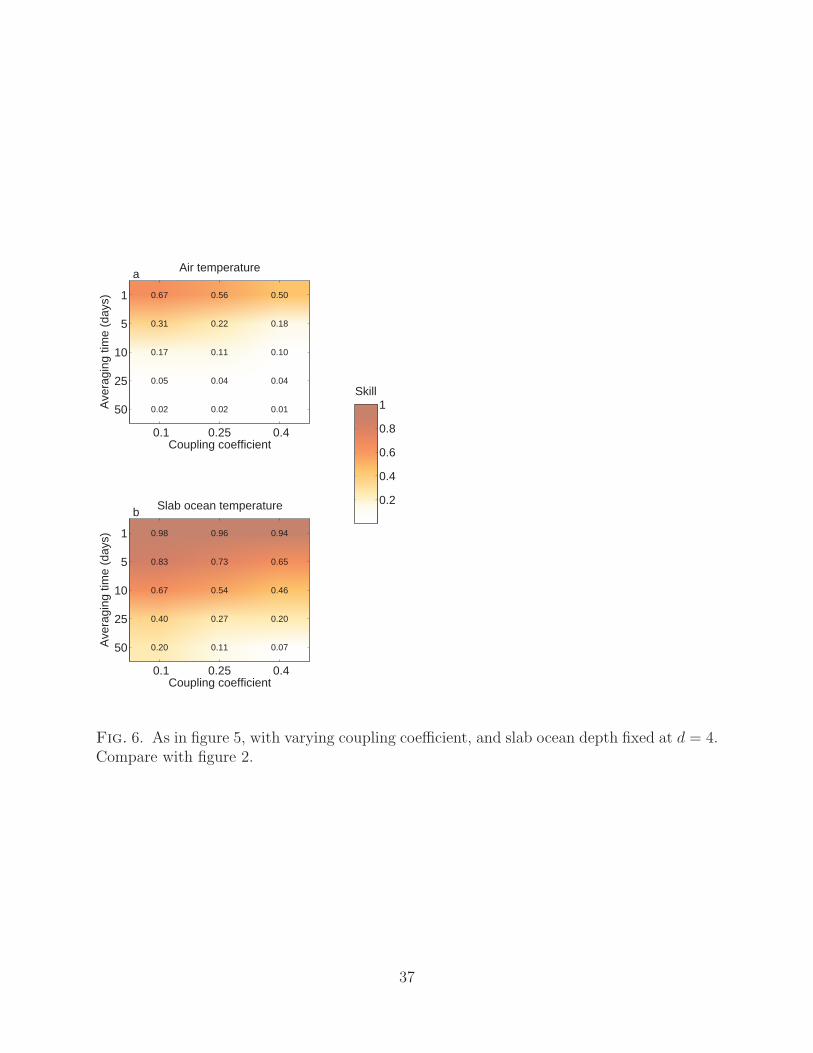
Skill as a function of averaging time and coupling strength, for fixed slab-ocean depth, is
shown in Fig. 6 (compare to QG model results in Fig. 2). Skill for air temperature decreases
as coupling increases, which is the opposite of that found in the QG experiments. Skill for
ocean temperature decreases as coupling increases, which is consistent with that found for
the QG model. In summary, compared to the QG results, the BB system shows a similar
response to varying slab-ocean depth, the same response to coupling for the ocean, but the
opposite response to coupling in the atmosphere.
14
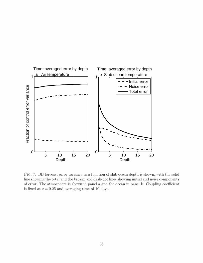
c. Decomposing error: accumulation of noise and initial condition
We can gain further understanding of the dependence of reconstruction skill on coupling
strength and slab ocean depth from the error evolution equation (4) for the BB system. As
discussed in section 2b, the error covariance evolution depends on two factors: the initial
error at the start of an assimilation cycle and the accumulation of stochastic noise. We
note that although the initial error depends on the noise error, observation error, and data
assimilation system, the decomposition discussed here provides a useful perspective on the
relative importance of initial error to accumulating noise in the forecast. Figure 7 shows the
total error broken into these two terms as a function of slab-ocean depth. Assimilation is
performed as for the previous assimilation experiments; the converged solution for the total
error and its two component parts are plotted separately for the atmosphere and ocean.
For the atmosphere, the fraction of the error variance attributable to initial error decreases
slightly with increasing depth, while the part proportional to noise accumulation increases.
The increase due to noise accumulation dominates, so that the total error increases with
depth. For the ocean, the fraction of error due to noise decreases strongly with increasing
slab-ocean depth, whereas the fraction due to initial error peaks at small depth and decreases
gradually with depth so that it dominates the total error for large depth.
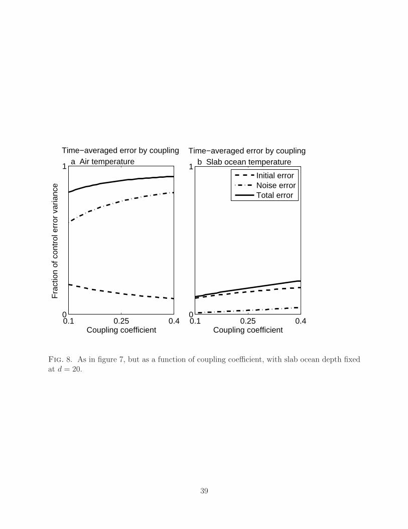
Results for sensitivity to the coupling strength are shown in Fig. 8. For the atmosphere
noise error dominates over initial-condition error, as is the case for the depth experiments.
For the ocean, initial-condition error dominates, as for the depth experiments. For the ocean,
a notable difference from the depth experiments is that the noise error increases slowly with
coupling, whereas it decreases sharply with increasing depth. A physical interpretation of
15
these sensitivity results is that deeper slab oceans are less sensitive to atmospheric noise
due to increased thermal inertia, whereas stronger coupling increases the amount of noise
introduced from the atmosphere, but this latter effect is weak compared to initial condition
error.
4. Conclusions
The problem of reconstructing past climates from time-average observations has been
explored within an idealized framework for midlatitude atmosphere-ocean interaction. A QG
model coupled to a slab ocean was used to explore the hypotheses that skill in reconstructions
will increase when (1) the depth of the slab ocean increases, and (2) the strength of the
coupling increases. Results show that for increasing slab-ocean depth ocean skill increases
as expected, but skill in the atmosphere does not. Skill increases slightly in the atmosphere
for stronger coupling, but it decreases in the ocean. For both atmosphere and ocean, skill
decreases with increasing observation averaging time.
The average freely-evolving behavior of the QG system was shown to correspond well
to that of a simple two-variable linear stochastic model for midlatitude air–sea interaction
(the BB system). Results for assimilation experiments for this system are similar to QG for
sensitivity to slab-ocean depth, but not for coupling. An analytical expression for the BB
error covariance forecast evolution helps explain these results. The atmosphere loses state-
dependent skill faster than the ocean because the stochastic component of error accumulates
more quickly than in the ocean. Moreover, the fraction of the total atmospheric forecast
error variance due to stochastic noise increases with both slab-ocean depth and coupling
16
strength. That is, in the BB system, noise controls the solution more than initial-condition
error. A physical interpretation of these results is that the ocean becomes thermally stiffer for
increasing depth and coupling, so that noise “accumulates” in the atmosphere. For changes
in coupling, responses are not consistent between the models. We speculate that advection
of atmospheric anomalies combined with nonlinearities in the QG model cause this difference
in behavior.
What do these results imply for climate reconstructions from data assimilation? Recon-
structions from data assimilation are possible even when the “skill” of the forecast model
at assimilation time, which was explored here, is no better than climatology. In this case,
data assimilation can still be an improvement over statistical reconstruction, where climate
covariances are a strong function of mean state, for example. The simple mixed-layer models
considered here lack skill beyond a few months. Therefore, for the problem of paleoclimate
data assimilation, a prerequisite is to establish that there is skill on longer time scales. This
might happen with a model coupled to more slowly varying components such as the deep
ocean or ice sheets. However, two more criteria must also be met: 1) the component’s fidelity
to nature must be quantified, and 2) there should be a strong relationship between the slow
component and the observed proxy.
Acknowledgments.
This research was sponsored by the National Science Foundation through grant 0902500,
awarded to the University of Washington. The first author was also by supported by fel-
lowships from National Defense Science and Engineering Graduate fellowship program and
17

Achievement Rewards for College Scientists. The first author thanks Nils Napp for insightful
conversations on stochastic calculus.
18
APPENDIX
Development and evaluation of error covariance.
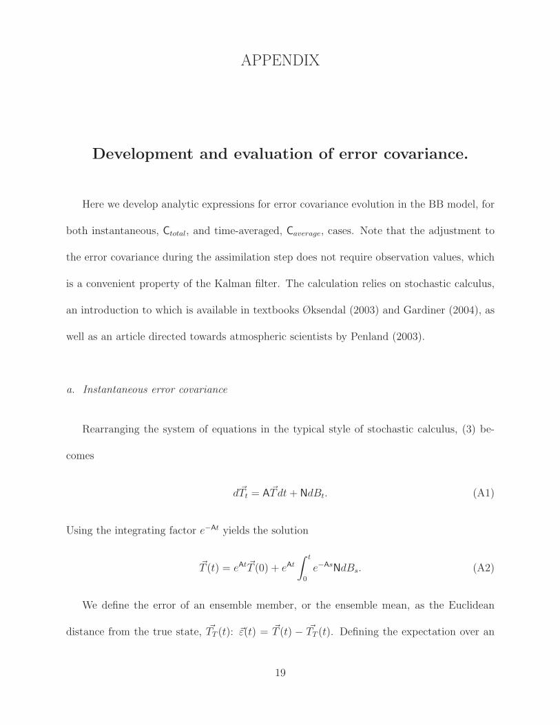
Here we develop analytic expressions for error covariance evolution in the BB model, for
both instantaneous, Ctotal, and time-averaged, Caverage, cases. Note that the adjustment to
the error covariance during the assimilation step does not require observation values, which
is a convenient property of the Kalman filter. The calculation relies on stochastic calculus,
an introduction to which is available in textbooks Øksendal (2003) and Gardiner (2004), as
well as an article directed towards atmospheric scientists by Penland (2003).
a. Instantaneous error covariance
Rearranging the system of equations in the typical style of stochastic calculus, (3) be-
comes
d~Tt = A~Tdt + NdBt. (A1)
Using the integrating factor e−At yields the solution
~T (t) = eAt ~T (0) + eAt
∫ t
0
e−AsNdBs. (A2)
We define the error of an ensemble member, or the ensemble mean, as the Euclidean
distance from the true state, ~TT (t): ~ε(t) = ~T (t) − ~TT (t). Defining the expectation over an
19
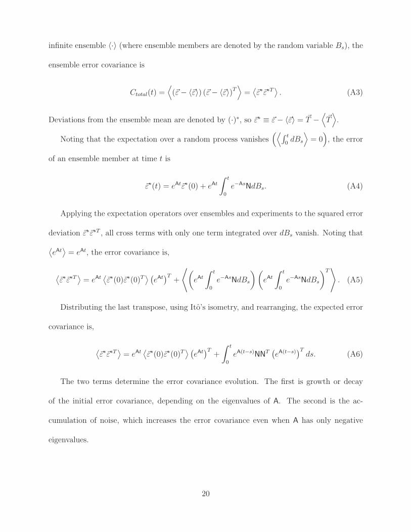
infinite ensemble 〈·〉 (where ensemble members are denoted by the random variable Bs), the
ensemble error covariance is
Ctotal(t) =⟨
(~ε − 〈~ε〉) (~ε − 〈~ε〉)T⟩
=⟨
~ε∗~ε∗T⟩
. (A3)
Deviations from the ensemble mean are denoted by (·)∗, so ~ε∗ ≡ ~ε − 〈~ε〉 = ~T −⟨
~T⟩
.
Noting that the expectation over a random process vanishes(⟨
∫ t
0dBs
⟩
= 0)
, the error
of an ensemble member at time t is
~ε∗(t) = eAt~ε∗(0) + eAt
∫ t
0
e−AsNdBs. (A4)
Applying the expectation operators over ensembles and experiments to the squared error
deviation ~ε∗~ε∗T , all cross terms with only one term integrated over dBs vanish. Noting that
⟨
eAt⟩
= eAt, the error covariance is,
⟨
~ε∗~ε∗T⟩
= eAt⟨
~ε∗(0)~ε∗(0)T⟩ (
eAt)T
+
⟨
(
eAt
∫ t
0
e−AsNdBs
) (
eAt
∫ t
0
e−AsNdBs
)T⟩
. (A5)
Distributing the last transpose, using Ito’s isometry, and rearranging, the expected error
covariance is,
⟨
~ε∗~ε∗T⟩
= eAt⟨
~ε∗(0)~ε∗(0)T⟩ (
eAt)T
+
∫ t
0
eA(t−s)NN
T(
eA(t−s))T
ds. (A6)
The two terms determine the error covariance evolution. The first is growth or decay
of the initial error covariance, depending on the eigenvalues of A. The second is the ac-
cumulation of noise, which increases the error covariance even when A has only negative
eigenvalues.
20
b. Error covariance of time-averaged states
The error of the time-averaged state is equal to the time-averaged error. Therefore, the
error of a time-averaged state is given by
ε∗ =1
L
∫ L
0
ε∗(t)dt =1
L
∫ L
0
(
eAt~ε∗(0) + eAt
∫ t
0
e−AsNdBs
)
dt, (A7)
where · denotes a time average and vector symbols are omitted for clarity.
Squaring the quantity above and applying the expectation operator, the cross-terms
cancel as they did for the instantaneous error covariance, leaving
⟨
ε∗ε∗T⟩
=1
L2
∫ L
0
eAtε∗(0)dt
(∫ L
0
eAtε∗(0)dt
)T
+1
L2
(∫ L
0
(∫ t
0
eA(t−s)NdBs
)
dt
)(∫ L
0
(∫ t
0
eA(t−s)NdBs
)
dt
)T
. (A8)
Switching the order of integration and using Ito’s isometry again yields
⟨
ε∗ε∗T⟩
=1
L2
∫ L
0
eAtε∗(0)dt
(∫ L
0
eAtε∗(0)dt
)T
+1
L2
∫ L
0
(∫ L
s
eA(t−s)Ndt
) (∫ L
s
eA(t−s)Ndt
)T
ds. (A9)
The error covariance of time-averaged states evolves in an analogous fashion to the instan-
taneous states, depending on initial error and the accumulation of stochastic noise.
c. Evaluating the integrals
Since A is linear and constant for the BB model, the evaluation of the covariance integrals
is straightforward. The calculation will be shown only once, since all other terms can be
solved in a similar manner.
21
The first term in the instantaneous error covariance equation (A6) can be evaluated
directly. For the second term, we define M(t, s) = eA(t−s), so that the second term can be
written as
∫ t
0
M(t, s)NNTM(t, s)T ds = N2
∫ t
0m2
11ds∫ t
0m21m11ds
∫ t
0m21m11ds
∫ t
0m2
21ds
, (A10)
where the elements of M are mii and depend on t and s. We calculate the elements of M
by doing an eigenvalue decomposition of A, since if A = VDV−1 then eA(t−s) = VeD(t−s)V−1.
Then distributing and rearranging the elements of V and D yields
M(t, s) =1
det(V)
v11v22ed1(t−s) − v12v21e
d2(t−s) −v11v12ed1(t−s) + v12v11e
d2(t−s)
v21v22ed1t(t−s) − v21v22e
d2(t−s) −v12v21ed1(t−s) + v22v11e
d2(t−s)
. (A11)
The integral of each element of (A11) has three exponential terms: e2d1(t−s), e(d1+d2)(t−s),
and e2d2(t−s), with all other quantities constant. This leaves the sum of many integrals of
the form∫ t
0ea(t−s)ds for a = 2d1, d1 + d2, and 2d2, which have solution
∫ t
0
ea(t−s)ds =1
a
(
eat − 1)
. (A12)
Evaluating the error covariance of time-averaged states is similar to evaluating the instan-
taneous error covariances. The first term of (A9) is rewritten by distributing transposes and
integrating (note that I is the identity matrix and (·)−T indicates an inverse and a transpose),
1
L2
∫ L
0
eAtε∗(0)dt
(∫ L
0
eAtε(0)dt
)T
=1
L2
(∫ L
0
eAtdt
)
ε(0)ε∗(0)T
(∫ L
0
(
eAt)T
dt
)
(A13)
=1
L2A−1
(
eAL − I)
ε∗(0)ε∗(0)T(
eAL − I)T
A−T . (A14)
22
For the second term, we return to M and its elements,
1
L2
∫ L
0
(∫ L
s
M(t, s)Ndt
) (∫ L
s
M(t, s)Ndt
)T
ds
=N2
L2
∫ L
0
(
∫ L
sm11(t, s)dt
)2∫ L
sm11(t, s)dt
∫ L
sm21(t, s)dt
∫ L
sm21(t, s)dt
∫ L
sm11(t, s)dt
(
∫ L
sm21(t, s)dt
)2
ds. (A15)
As in the instantaneous case, each of the elements of this matrix is the product of integrals
over exponential terms. Each of the exponential integral parts can be broken down into
∫ L
0
(∫ L
s
ea(t−s)dt
∫ L
s
eb(t−s)dt
)
ds
=1
ab
(
−1
a + b
(
1 − e(a+b)L)
+1
a
(
1 − eaL)
+1
b
(
1 − ebL)
+ L
)
. (A16)
Matlab implementation allows calculation of the error covariance of quantities averaged over
time L from an initial error covariance. An example integration of the system is shown in
Fig. 4.
23
REFERENCES
Anderson, J., T. Hoar, K. Raeder, H. Liu, N. Collins, R. Torn, and A. Avellano, 2009:
The data assimilation research testbed: A community facility. Bull. Amer. Meteor. Soc.,
90 (9), 1283–1296.
Anderson, J. L., 2001: An ensemble adjustment Kalman filter for data assimilation. Mon.
Wea. Rev., 129 (12), 2884–2903.
Barsugli, J. J. and D. S. Battisti, 1998: The basic effects of atmosphere–ocean thermal
coupling on midlatitude variability. J. Atmos. Sci., 55 (4), 477–493.
Boer, G. J., 2000: A study of atmosphere-ocean predictability on long time scales. Cli-
mate Dyn., 16 (6), 469–477.
Boer, G. J. and S. J. Lambert, 2008: Multi-model decadal potential predictability of precip-
itation and temperature. Geophys. Res. Lett., 35 (5), L05 706.
Collins, M., 2002: Climate predictability on interannual to decadal time scales: the initial
value problem. Climate Dyn., 19 (8), 671–692.
Davis, R., 1976: Predictability of sea surface temperature and sea level pressure anomalies
over the North Pacific Ocean. J. Phys. Oceanogr., 6 (3), 249–266.
Deser, C., M. A. Alexander, and M. S. Timlin, 2003: Understanding the persistence of sea
surface temperature anomalies in midlatitudes. J. Climate, 16 (1), 57–72.
24
Dirren, S. and G. J. Hakim, 2005: Toward the assimilation of time-averaged observations.
Geophys. Res. Lett., 32 (4), L04 804.
Frankignoul, C. and K. Hasselmann, 1977: Stochastic climate models. Part II: Application
to sea-surface temperature anomalies and thermocline variability. Tellus, 29 (4), 289–305.
Gardiner, C. W., 2004: Handbook Of Stochastic Methods: for Physics, Chemistry And The
Natural Sciences. 3rd ed., Springer, 415 pp.
Gaspari, G. and S. E. Cohn, 1999: Construction of correlation functions in two and three
dimensions. Quart. J. Roy. Meteor. Soc., 125, 723–757.
Griffies, S. M. and K. Bryan, 1997: A predictability study of simulated North Atlantic
multidecadal variability. Climate Dyn., 13 (7-8), 459–487.
Grotzner, A., M. Latif, A. Timmermann, and R. Voss, 1999: Interannual to decadal pre-
dictability in a coupled ocean-atmosphere general circulation model. J. Climate, 12 (8),
2607–2624.
Hakim, G. J., 2000: Role of nonmodal growth and nonlinearity in cyclogenesis initial-value
problems. J. Atmos. Sci., 57 (17), 2951–2967.
Hasselmann, K., 1976: Stochastic climate models Part I. Theory. Tellus, 28 (6), 473–485.
Hoskins, B. and N. West, 1979: Baroclinic waves and frontogenesis. Part II: Uniform poten-
tial vorticity jet flows—Cold and warm fronts. J. Atmos. Sci, 36, 1663–1680.
Huntley, H. S. and G. J. Hakim, 2009: Assimilation of time-averaged observations in a
quasi-geostrophic atmospheric jet model. Climate Dyn., 1–15.
25
Jones, P. D., et al., 2009: High-resolution palaeoclimatology of the last millennium: A review
of current status and future prospects. Holocene, 19 (1), 3–49.
Koenigk, T. and U. Mikolajewicz, 2009: Seasonal to interannual climate predictability in mid
and high northern latitudes in a global coupled model. Climate Dyn., 32 (6), 783–798.
Latif, M., 1998: Dynamics of interdecadal variability in coupled ocean-atmosphere models.
J. Climate, 11 (4), 602–624.
Latif, M., M. Collins, H. Pohlmann, and N. Keenlyside, 2006: A review of predictability
studies of Atlantic sector climate on decadal time scales. J. Climate, 19 (23), 5971–5987.
Mann, M. E., R. S. Bradley, and M. K. Hughes, 1999: Northern hemisphere temperatures
during the past millennium: Inferences, uncertainties, and limitations. Geophys. Res. Lett.,
26 (6), 759–762.
Meehl, G. A., et al., 2009: Decadal prediction: Can it be skillful? Bull. Amer. Meteor. Soc.,
90 (10), 1467–1485.
Øksendal, B. K., 2003: Stochastic Differential Equations: An Introduction With Applica-
tions. 6th ed., Springer, 360 pp.
Penland, C., 2003: A stochastic approach to nonlinear dynamics: A review (extended version
of the article - ”Noise out of chaos and why it won’t go away”). Bull. Amer. Meteor. Soc.,
84 (7), 925–925.
Pohlmann, H., M. Botzet, M. Latif, A. Roesch, M. Wild, and P. Tschuck, 2004: Estimating
the decadal predictability of a coupled AOGCM. J. Climate, 17 (22), 4463–4472.
26
Saravanan, R., G. Danabasoglu, S. C. Doney, and J. C. McWilliams, 2000: Decadal vari-
ability and predictability in the midlatitude oceanatmosphere system. J. Climate, 13 (6),
1073–1097.
Saravanan, R. and J. C. McWilliams, 1998: Advective oceanatmosphere interaction: An
analytical stochastic model with implications for decadal variability. J. Climate, 11 (2),
165–188.
Schopf, P. S., 1985: Modeling tropical sea-surface temperature: Implications of various
atmospheric responses. Coupled ocean–atmosphere models, J. C. J. Nihoul, Ed., Elsevier
Science Publishers B.V., Elsevier Oceanography Series, Vol. 40, 727–734.
Scott, R. B., 2003: Predictability of SST in an idealized, one-dimensional, coupled
atmosphere–ocean climate model with stochastic forcing and advection. J. Climate,
16 (2), 323–335.
27

List of Tables
1 Values of parameters used as baseline in the BB and QG models. 28
28
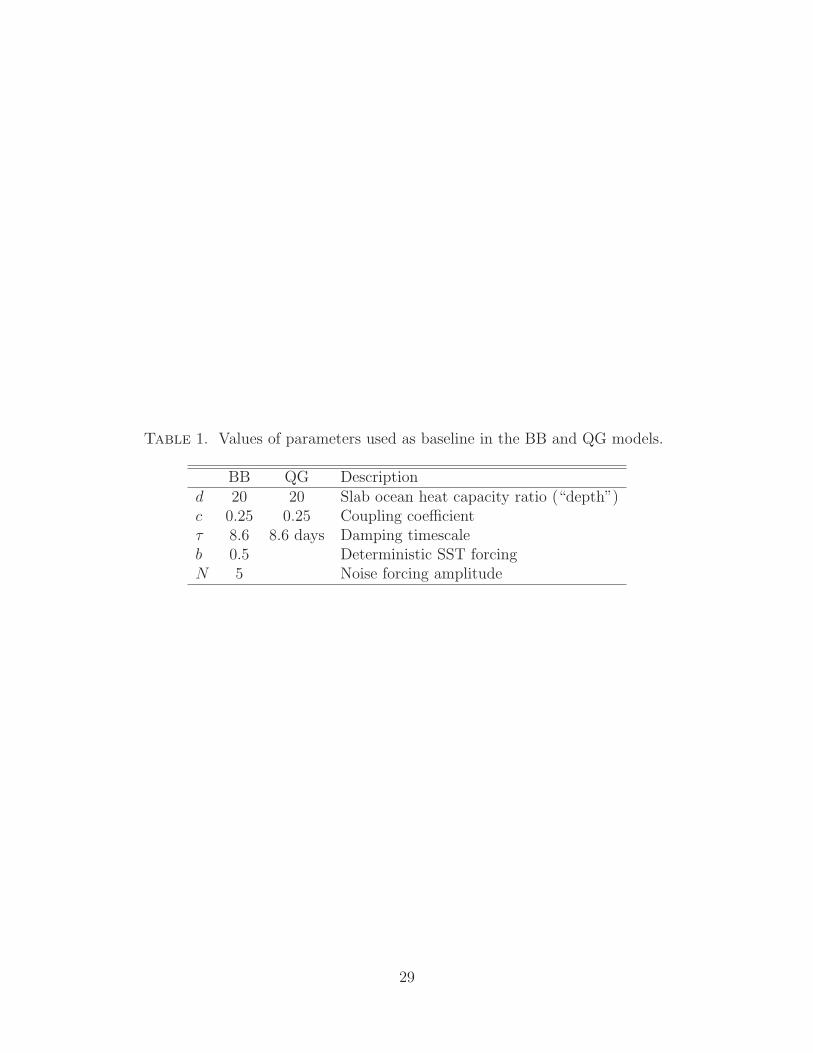
Table 1. Values of parameters used as baseline in the BB and QG models.
BB QG Descriptiond 20 20 Slab ocean heat capacity ratio (“depth”)c 0.25 0.25 Coupling coefficientτ 8.6 8.6 days Damping timescaleb 0.5 Deterministic SST forcingN 5 Noise forcing amplitude
29
List of Figures
1 Skill for QG data assimilation system (ensemble error variance at assimilation
time normalized by control error variance) is shown, as a function of averaging
time and slab ocean depth. Panel a is the atmosphere and panel b is the ocean.
Coupling coefficient is c = 0.25. 31
2 As in figure 1, for varying coupling coefficient with slab ocean depth fixed at
d=4. 32
3 Cospectral analysis of surface air and slab ocean temperature from QG model
and the corresponding cospectra from BB model are shown. The power spec-
tral density is shown in panel a for the surface air temperature and in panel
c for the slab ocean temperature. The real part of their cospectrum is shown
in panel b, and the imaginary part is shown in panel d. The coherence of
the surface air temperature and slab ocean temperature for the QG model
is shown in panel e; BB model coherence is always one because the model is
linear. The phase lag of the slab ocean behind the surface air temperature is
shown in panel f. A histogram for each frequency shows the relative frequency
of spectral lines from QG model gridpoints. The contour interval is 0.1. The
total power spectral density vertical integral for each frequency in each panel
is one. 33
30
4 The error variance of time-averaged states for the BB data assimilation system
is shown, with the atmosphere in the left panels (a, c, and e) and the ocean
in the right panels (b, d, and f). The top panels (a and b) show the “Spinup”
phase, where error grows asymptotically towards an equilibrium value without
assimilating observations. The middle panels (c and d) show the “Control,”
case, where error stays at the equilibrium value without assimilation. The
bottom panels (e and f) show sawtooth plots (with both forecast and analysis
error variance) for the “Assimilation” case, where observations with error
variance of 1/10 of final spinup variance are assimilated. Model parameters
are c = 0.4, d = 20, and an averaging time of 10 days. 34
5 Skill for the BB data assimilation system (error variance at assimilation time
normalized by control error variance) is shown, as a function of averaging time
and slab ocean depth, with the atmosphere in panel a and ocean in panel b.
Coupling coefficient is fixed at c = 0.25. Compare with figure 1. 35
6 As in figure 5, with varying coupling coefficient, and slab ocean depth fixed
at d = 4. Compare with figure 2. 36
7 BB forecast error variance as a function of slab ocean depth is shown, with the
solid line showing the total and the broken and dash-dot lines showing initial
and noise components of error. The atmosphere is shown in panel a and the
ocean in panel b. Coupling coefficient is fixed at c = 0.25 and averaging time
of 10 days. 37
8 As in figure 7, but as a function of coupling coefficient, with slab ocean depth
fixed at d = 20. 38
31
Skill
0.2
0.4
0.6
0.8
1
Ave
ragi
ng ti
me
(day
s)
Slab ocean temperature
0.98
0.66
0.37
0.07
−0.01
0.97
0.82
0.64
0.27
0.06
0.95
0.89
0.81
0.67
0.49
Slab ocean heat capacity ratio
b
1 4 20
1
5
10
25
50
Ave
ragi
ng ti
me
(day
s)
Surface air potential temperature
0.94
0.38
0.21
0.05
−0.02
0.94
0.34
0.22
0.08
0.00
0.95
0.26
0.13
0.04
0.02
Slab ocean heat capacity ratio
a
1 4 20
1
5
10
25
50
Fig. 1. Skill for QG data assimilation system (ensemble error variance at assimilation timenormalized by control error variance) is shown, as a function of averaging time and slabocean depth. Panel a is the atmosphere and panel b is the ocean. Coupling coefficient isc = 0.25.
32
Skill
0.2
0.4
0.6
0.8
1
Ave
ragi
ng ti
me
(day
s)
Slab ocean temperature
0.95
0.84
0.71
0.35
0.11
0.97
0.82
0.64
0.27
0.06
0.98
0.81
0.65
0.16
−0.03
Coupling coefficient
b
0.1 0.25 0.4
1
5
10
25
50
Ave
ragi
ng ti
me
(day
s)
Surface air potential temperature
0.87
0.28
0.10
0.00
−0.01
0.94
0.34
0.22
0.08
0.00
0.97
0.36
0.32
0.04
−0.04
Coupling coefficient
a
0.1 0.25 0.4
1
5
10
25
50
Fig. 2. As in figure 1, for varying coupling coefficient with slab ocean depth fixed at d=4.
33
Frequency (days−1)
Phasef
10−3
10−2
0
0.1 0.2 0.3 0.4 0.5 0.6 0.7 0.8 0.9 1
Frequency (days−1)
Coherencee
10−3
10−2
0
0.2
0.4
0.6
0.8
1
Imaginary cospectrad
0
1
2
3
4
Real cospectrab
0
2
4
6P
ower
spe
ctra
l den
sity
Surface air temperature PSDa
0
2
4
6
8
Pow
er s
pect
ral d
ensi
ty
Slab ocean temperature PSDc
0
1
2
3
4
5
QG pointsBB
π
−π
−π2
π2
Fig. 3. Cospectral analysis of surface air and slab ocean temperature from QG model andthe corresponding cospectra from BB model are shown. The power spectral density is shownin panel a for the surface air temperature and in panel c for the slab ocean temperature. Thereal part of their cospectrum is shown in panel b, and the imaginary part is shown in paneld. The coherence of the surface air temperature and slab ocean temperature for the QGmodel is shown in panel e; BB model coherence is always one because the model is linear.The phase lag of the slab ocean behind the surface air temperature is shown in panel f. Ahistogram for each frequency shows the relative frequency of spectral lines from QG modelgridpoints. The contour interval is 0.1. The total power spectral density vertical integral foreach frequency in each panel is one.
34
150 200 250 3000
0.5
1
Assimilation f
150 200 250 3000
5
10
15
20
25 Assimilation
Err
or v
aria
nce
(K2 ) e
150 200 250 3000
0.5
1
Control d
150 200 250 3000
5
10
15
20
25 Control
Err
or v
aria
nce
(K2 ) c
0 50 100 1500
0.5
1
Slab ocean temperature
Spinup
Time (days)
b
0 50 100 1500
5
10
15
20
25Atmosphere temperature
SpinupE
rror
var
ianc
e (K
2 )
Time (days)
a
Fig. 4. The error variance of time-averaged states for the BB data assimilation systemis shown, with the atmosphere in the left panels (a, c, and e) and the ocean in the rightpanels (b, d, and f). The top panels (a and b) show the “Spinup” phase, where errorgrows asymptotically towards an equilibrium value without assimilating observations. Themiddle panels (c and d) show the “Control,” case, where error stays at the equilibriumvalue without assimilation. The bottom panels (e and f) show sawtooth plots (with bothforecast and analysis error variance) for the “Assimilation” case, where observations witherror variance of 1/10 of final spinup variance are assimilated. Model parameters are c = 0.4,d = 20, and an averaging time of 10 days.
35

Skill
0.2
0.4
0.6
0.8
1Ave
ragi
ng ti
me
(day
s)
Air temperature
0.60
0.25
0.13
0.03
0.01
0.56
0.22
0.11
0.04
0.02
0.54
0.18
0.08
0.03
0.02
Slab ocean heat capacity ratio
a
1 4 20
1
5
10
25
50
Ave
ragi
ng ti
me
(day
s)
Slab ocean temperature
0.90
0.52
0.30
0.08
0.02
0.96
0.73
0.54
0.27
0.11
0.98
0.89
0.80
0.61
0.43
Slab ocean heat capacity ratio
b
1 4 20
1
5
10
25
50
Fig. 5. Skill for the BB data assimilation system (error variance at assimilation time nor-malized by control error variance) is shown, as a function of averaging time and slab oceandepth, with the atmosphere in panel a and ocean in panel b. Coupling coefficient is fixed atc = 0.25. Compare with figure 1.
36
Skill
0.2
0.4
0.6
0.8
1Ave
ragi
ng ti
me
(day
s)
Air temperature
0.67
0.31
0.17
0.05
0.02
0.56
0.22
0.11
0.04
0.02
0.50
0.18
0.10
0.04
0.01
Coupling coefficient
a
0.1 0.25 0.4
1
5
10
25
50
Ave
ragi
ng ti
me
(day
s)
Slab ocean temperature
0.98
0.83
0.67
0.40
0.20
0.96
0.73
0.54
0.27
0.11
0.94
0.65
0.46
0.20
0.07
Coupling coefficient
b
0.1 0.25 0.4
1
5
10
25
50
Fig. 6. As in figure 5, with varying coupling coefficient, and slab ocean depth fixed at d = 4.Compare with figure 2.
37
5 10 15 200
1
Time−averaged error by depth Slab ocean temperature
Depth
b
Initial errorNoise errorTotal error
5 10 15 200
1
Fra
ctio
n of
con
trol
err
or v
aria
nce
Time−averaged error by depth Air temperature
Depth
a
Fig. 7. BB forecast error variance as a function of slab ocean depth is shown, with the solidline showing the total and the broken and dash-dot lines showing initial and noise componentsof error. The atmosphere is shown in panel a and the ocean in panel b. Coupling coefficientis fixed at c = 0.25 and averaging time of 10 days.
38
0.1 0.25 0.40
1
Time−averaged error by coupling Slab ocean temperature
Coupling coefficient
b
Initial errorNoise errorTotal error
0.1 0.25 0.40
1
Fra
ctio
n of
con
trol
err
or v
aria
nce
Time−averaged error by coupling Air temperature
Coupling coefficient
a
Fig. 8. As in figure 7, but as a function of coupling coefficient, with slab ocean depth fixedat d = 20.
39