IS THE US ECONOMY

RECOVERING?

Angela Sordello Christopher

Friedberg Can Shen

Hui LaiHui Wang

Fang Guo

OUTLINE

Introduction Original Data Pre Whitening Comparison of Models Modeling Model Validation Forecasting Conclusion

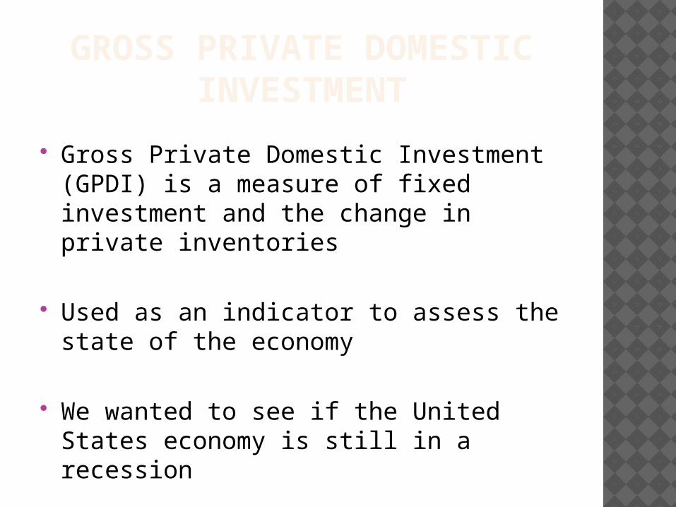
GROSS PRIVATE DOMESTIC INVESTMENT

Gross Private Domestic Investment (GPDI) is a measure of fixed investment and the change in private inventories

Used as an indicator to assess the state of the economy

We wanted to see if the United States economy is still in a recession

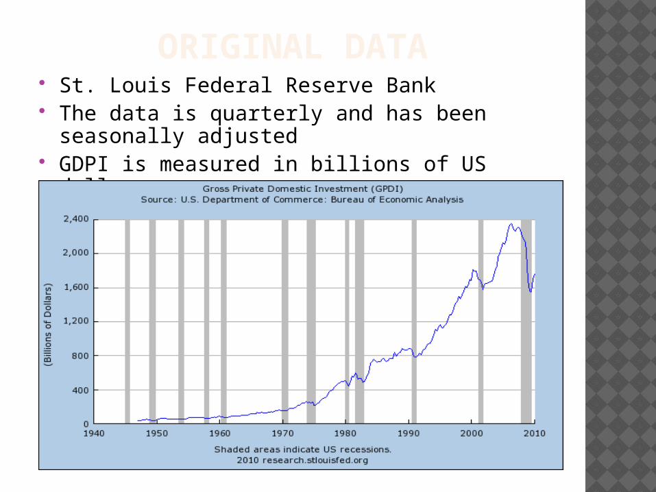
ORIGINAL DATA St. Louis Federal Reserve Bank The data is quarterly and has been seasonally

adjusted GDPI is measured in billions of US dollars

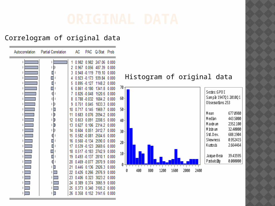
ORIGINAL DATA

0

10

20

30

40

50

60

70

0 400 800 1200 1600 2000 2400

Series: GPDISample 1947Q1 2010Q1Observations 253

Mean 677.0980Median 443.5000Maximum 2352.100Minimum 32.40000Std. Dev. 688.1904Skewness 0.952415Kurtosis 2.664464

Jarque-Bera 39.43595Probability 0.000000

Histogram of original data

Correlogram of original data

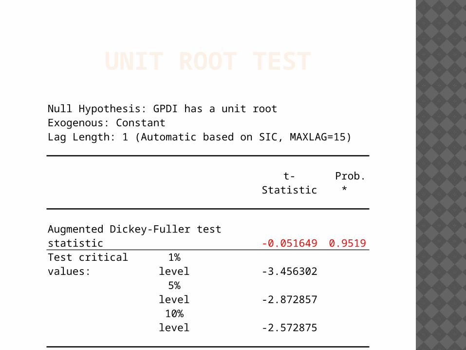
UNIT ROOT TEST

Null Hypothesis: GPDI has a unit rootExogenous: ConstantLag Length: 1 (Automatic based on SIC, MAXLAG=15)

t-Statistic   Prob.*

Augmented Dickey-Fuller test statistic -0.051649  0.9519Test critical values: 1% level -3.456302

5% level -2.87285710% level -2.572875

*MacKinnon (1996) one-sided p-values.

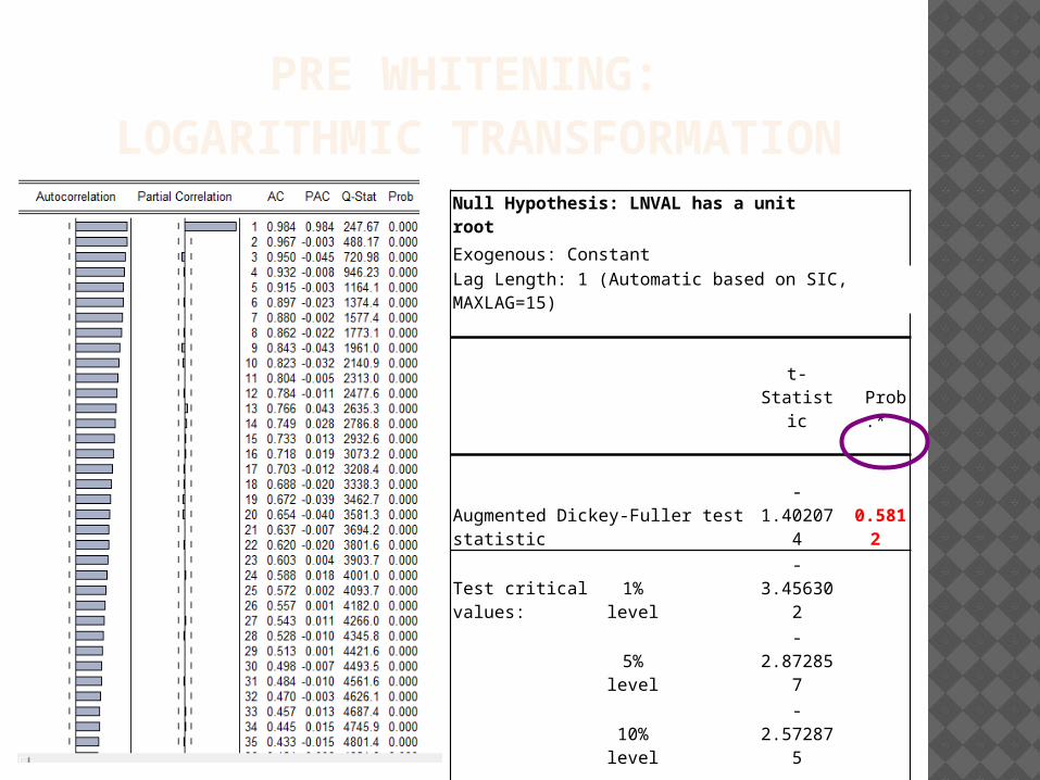
PRE WHITENING: LOGARITHMIC TRANSFORMATION

Null Hypothesis: LNVAL has a unit root

Exogenous: Constant

Lag Length: 1 (Automatic based on SIC, MAXLAG=15)

t-Statistic   Prob.*

Augmented Dickey-Fuller test statistic -1.402074  0.5812

Test critical values: 1% level -3.456302

5% level -2.872857

10% level -2.572875

*MacKinnon (1996) one-sided p-values.

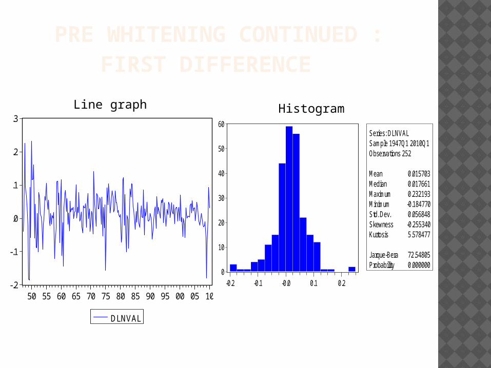
PRE WHITENING CONTINUED :FIRST DIFFERENCE

-.2

-.1

.0

.1

.2

.3

50 55 60 65 70 75 80 85 90 95 00 05 10

DLNVAL

0

10

20

30

40

50

60

-0.2 -0.1 -0.0 0.1 0.2

Series: DLNVALSample 1947Q1 2010Q1Observations 252

Mean 0.015703Median 0.017661Maximum 0.232193Minimum -0.184770Std. Dev. 0.056848Skewness -0.255340Kurtosis 5.578477

Jarque-Bera 72.54805Probability 0.000000

Line graph Histogram

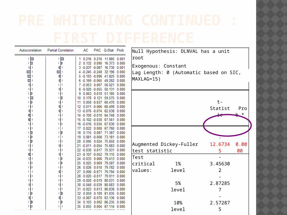
PRE WHITENING CONTINUED :FIRST DIFFERENCE

Null Hypothesis: DLNVAL has a unit root

Exogenous: ConstantLag Length: 0 (Automatic based on SIC, MAXLAG=15)

t-Statistic   Prob.*

Augmented Dickey-Fuller test statistic

-12.67345  0.0000

Test critical values:

1% level

-3.456302

5% level

-2.872857

10% level

-2.572875

*MacKinnon (1996) one-sided p-values.

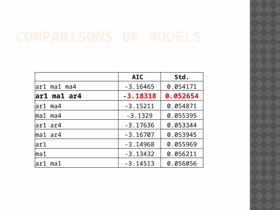
COMPARISONS OF MODELS

AIC Std.

ar1 ma1 ma4 -3.16465 0.054171

ar1 ma1 ar4 -3.18318 0.052654ar1 ma4 -3.15211 0.054871

ma1 ma4 -3.1329 0.055395

ar1 ar4 -3.17636 0.053344

ma1 ar4 -3.16707 0.053945

ar1 -3.14968 0.055969

ma1 -3.13432 0.056211

ar1 ma1 -3.14513 0.056056

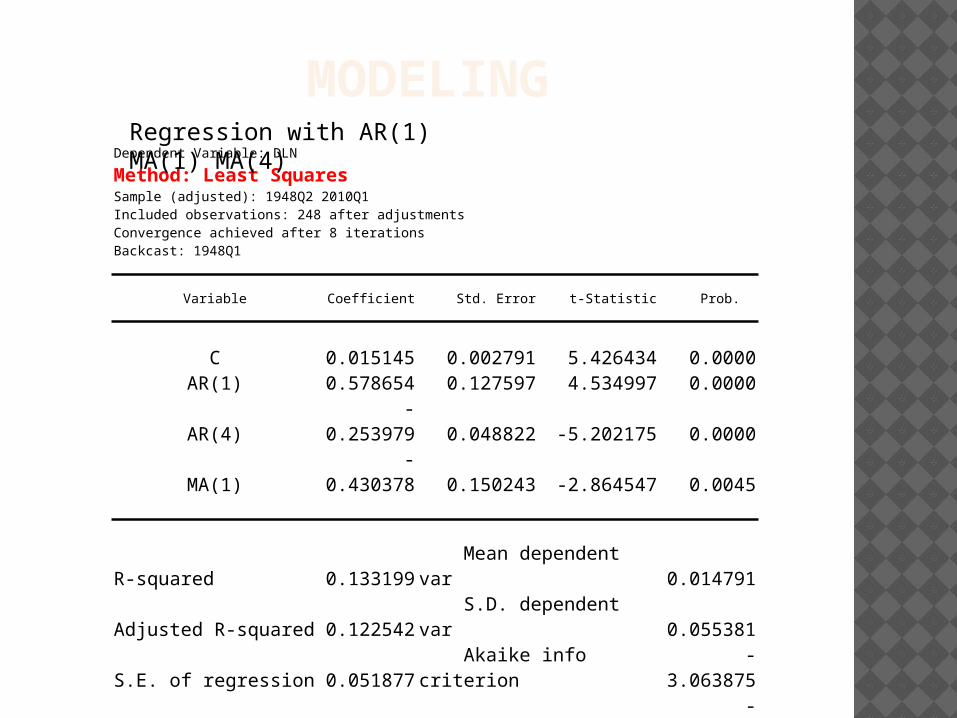
MODELINGDependent Variable: DLN

Method: Least SquaresSample (adjusted): 1948Q2 2010Q1Included observations: 248 after adjustmentsConvergence achieved after 8 iterationsBackcast: 1948Q1

Variable Coefficient Std. Error t-Statistic Prob.  

C 0.015145 0.002791 5.426434 0.0000AR(1) 0.578654 0.127597 4.534997 0.0000AR(4) -0.253979 0.048822 -5.202175 0.0000MA(1) -0.430378 0.150243 -2.864547 0.0045

R-squared 0.133199     Mean dependent var 0.014791Adjusted R-squared 0.122542     S.D. dependent var 0.055381S.E. of regression 0.051877     Akaike info criterion -3.063875Sum squared resid 0.656665     Schwarz criterion -3.007206Log likelihood 383.9205     F-statistic 12.49830Durbin-Watson stat 2.031919     Prob(F-statistic) 0.000000

Inverted AR Roots  .68-.46i      .68+.46i   -.39+.48i -.39-.48iInverted MA Roots       .43

Regression with AR(1) MA(1) MA(4)

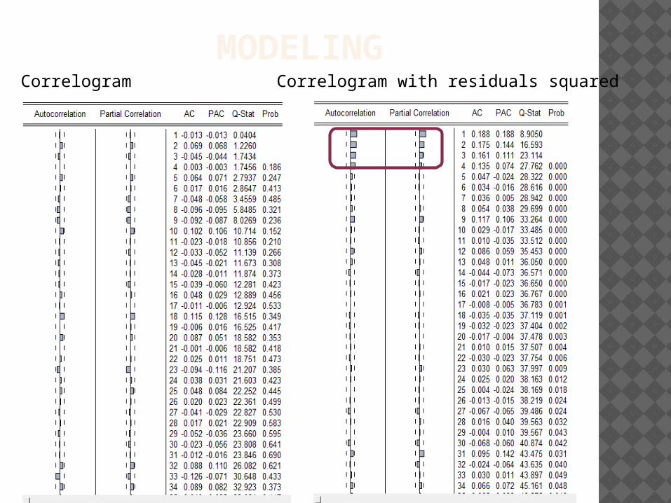
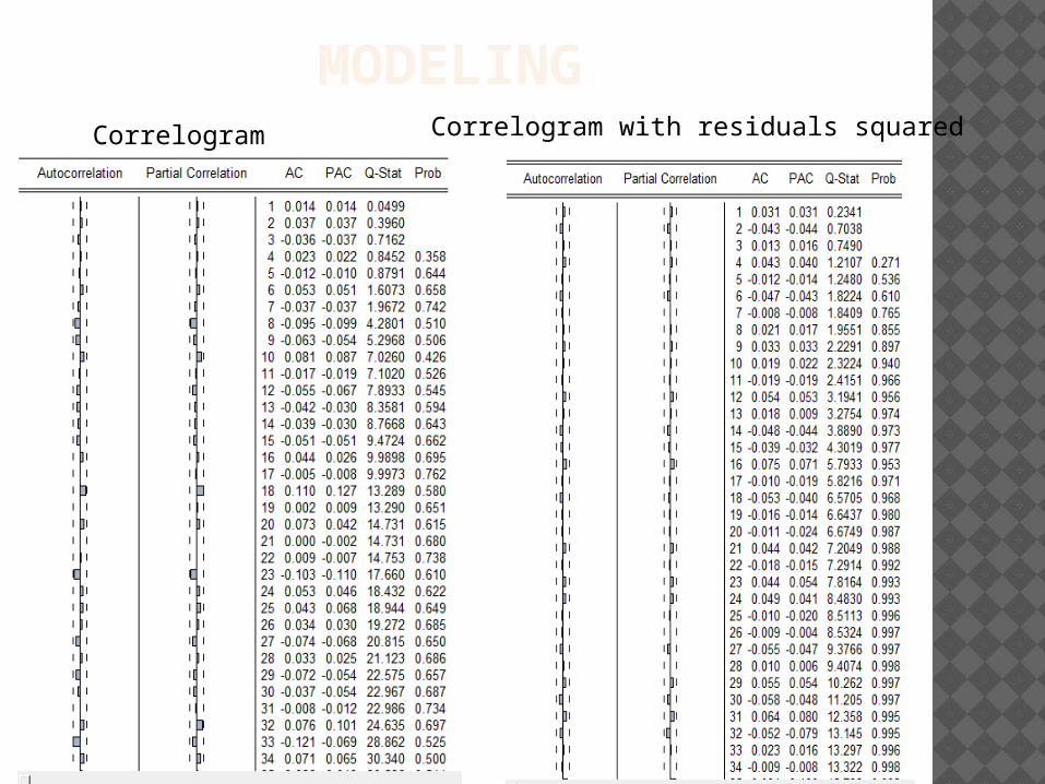
MODELINGCorrelogram Correlogram with residuals squared

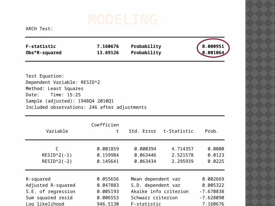
MODELINGARCH Test:

F-statistic 7.160676     Probability 0.000951Obs*R-squared 13.69126     Probability 0.001064

Test Equation:Dependent Variable: RESID^2Method: Least SquaresDate: Time: 15:25Sample (adjusted): 1948Q4 2010Q1Included observations: 246 after adjustments

Variable Coefficient Std. Error t-Statistic Prob.  

C 0.001859 0.000394 4.714357 0.0000RESID^2(-1) 0.159984 0.063446 2.521578 0.0123RESID^2(-2) 0.145641 0.063434 2.295939 0.0225

R-squared 0.055656     Mean dependent var 0.002669Adjusted R-squared 0.047883     S.D. dependent var 0.005322S.E. of regression 0.005193     Akaike info criterion -7.670838Sum squared resid 0.006553     Schwarz criterion -7.628090Log likelihood 946.5130     F-statistic 7.160676Durbin-Watson stat 2.036030     Prob(F-statistic) 0.000951

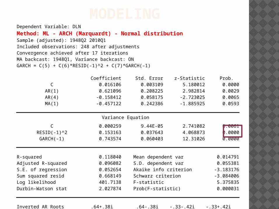
MODELINGDependent Variable: DLNMethod: ML - ARCH (Marquardt) - Normal distributionSample (adjusted): 1948Q2 2010Q1Included observations: 248 after adjustmentsConvergence achieved after 17 iterationsMA backcast: 1948Q1, Variance backcast: ONGARCH = C(5) + C(6)*RESID(-1)^2 + C(7)*GARCH(-1)

Coefficient Std. Error z-Statistic Prob.  C 0.016106 0.003109 5.180012 0.0000

AR(1) 0.621096 0.208225 2.982814 0.0029AR(4) -0.158412 0.058175 -2.723025 0.0065MA(1) -0.457122 0.242386 -1.885925 0.0593

Variance Equation

C 0.000259 9.44E-05 2.741082 0.0061RESID(-1)^2 0.153163 0.037643 4.068873 0.0000GARCH(-1) 0.743574 0.060403 12.31026 0.0000

R-squared 0.118040     Mean dependent var 0.014791Adjusted R-squared 0.096082     S.D. dependent var 0.055381S.E. of regression 0.052654     Akaike info criterion -3.183176Sum squared resid 0.668149     Schwarz criterion -3.084006Log likelihood 401.7138     F-statistic 5.375835Durbin-Watson stat 2.027874     Prob(F-statistic) 0.000031

Inverted AR Roots  .64+.38i      .64-.38i   -.33-.42i -.33+.42iInverted MA Roots       .46

MODELINGCorrelogram Correlogram with residuals squared

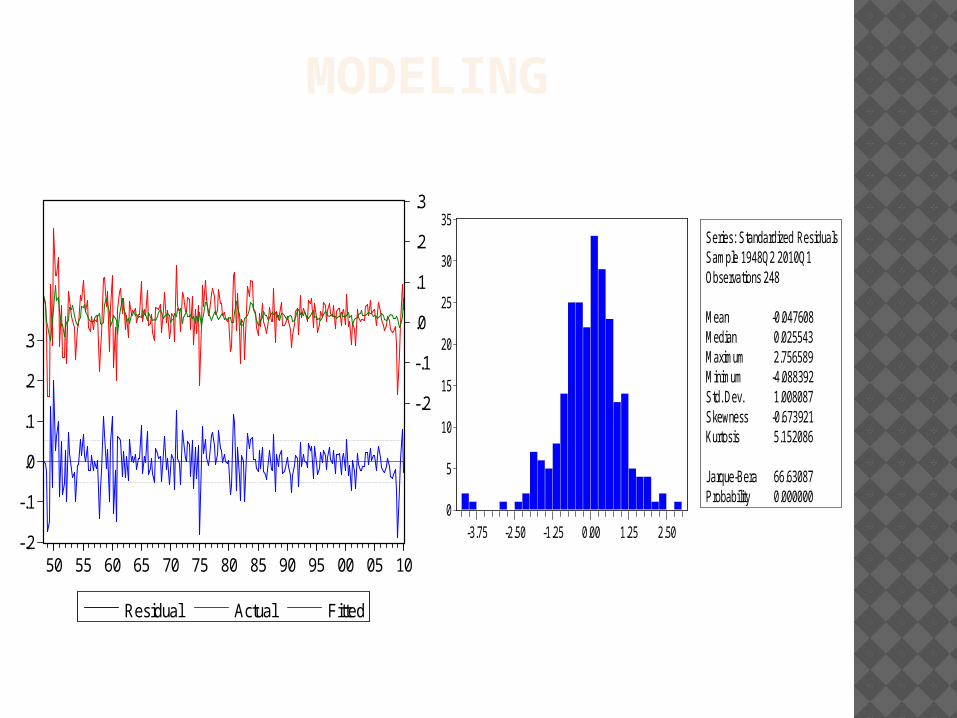
MODELING

-.2

-.1

.0

.1

.2

.3

-.2

-.1

.0

.1

.2

.3

50 55 60 65 70 75 80 85 90 95 00 05 10

Residual Actual Fitted

0

5

10

15

20

25

30

35

-3.75 -2.50 -1.25 0.00 1.25 2.50

Series: Standardized ResidualsSample 1948Q2 2010Q1Observations 248

Mean -0.047608Median 0.025543Maximum 2.756589Minimum -4.088392Std. Dev. 1.008087Skewness -0.673921Kurtosis 5.152086

Jarque-Bera 66.63087Probability 0.000000

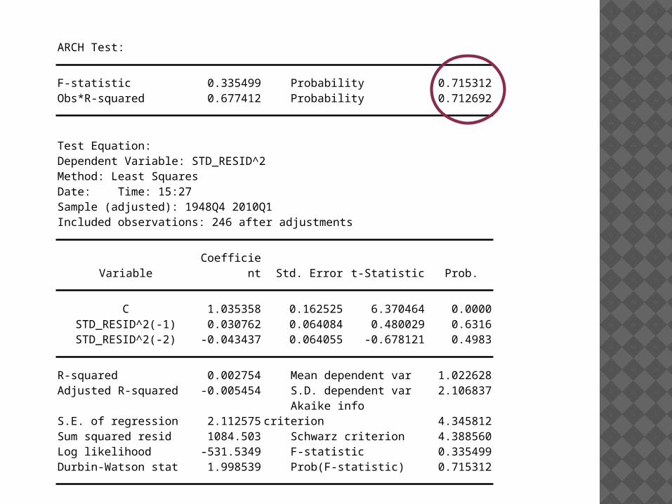
ARCH Test:

F-statistic 0.335499     Probability 0.715312Obs*R-squared 0.677412     Probability 0.712692

Test Equation:Dependent Variable: STD_RESID^2Method: Least SquaresDate: Time: 15:27Sample (adjusted): 1948Q4 2010Q1Included observations: 246 after adjustments

Variable Coefficient Std. Error t-Statistic Prob.  

C 1.035358 0.162525 6.370464 0.0000STD_RESID^2(-1) 0.030762 0.064084 0.480029 0.6316STD_RESID^2(-2) -0.043437 0.064055 -0.678121 0.4983

R-squared 0.002754     Mean dependent var 1.022628Adjusted R-squared -0.005454     S.D. dependent var 2.106837S.E. of regression 2.112575     Akaike info criterion 4.345812Sum squared resid 1084.503     Schwarz criterion 4.388560Log likelihood -531.5349     F-statistic 0.335499Durbin-Watson stat 1.998539     Prob(F-statistic) 0.715312

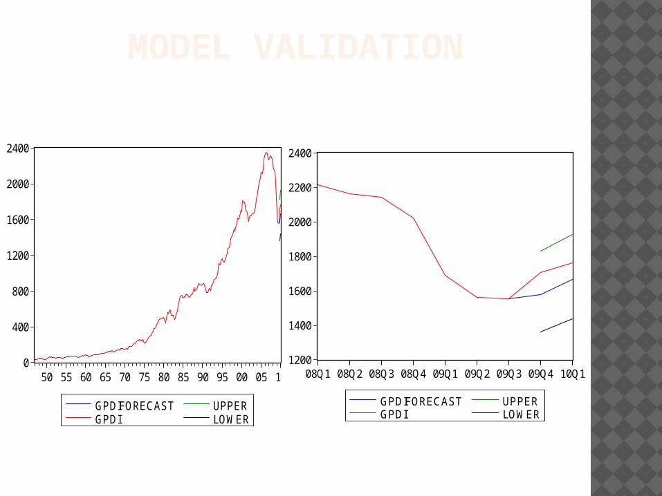
MODEL VALIDATION

0

400

800

1200

1600

2000

2400

50 55 60 65 70 75 80 85 90 95 00 05 10

GPDIFORECASTGPDI

UPPERLOWER

1200

1400

1600

1800

2000

2200

2400

08Q1 08Q2 08Q3 08Q4 09Q1 09Q2 09Q3 09Q4 10Q1

GPDIFORECASTGPDI

UPPERLOWER

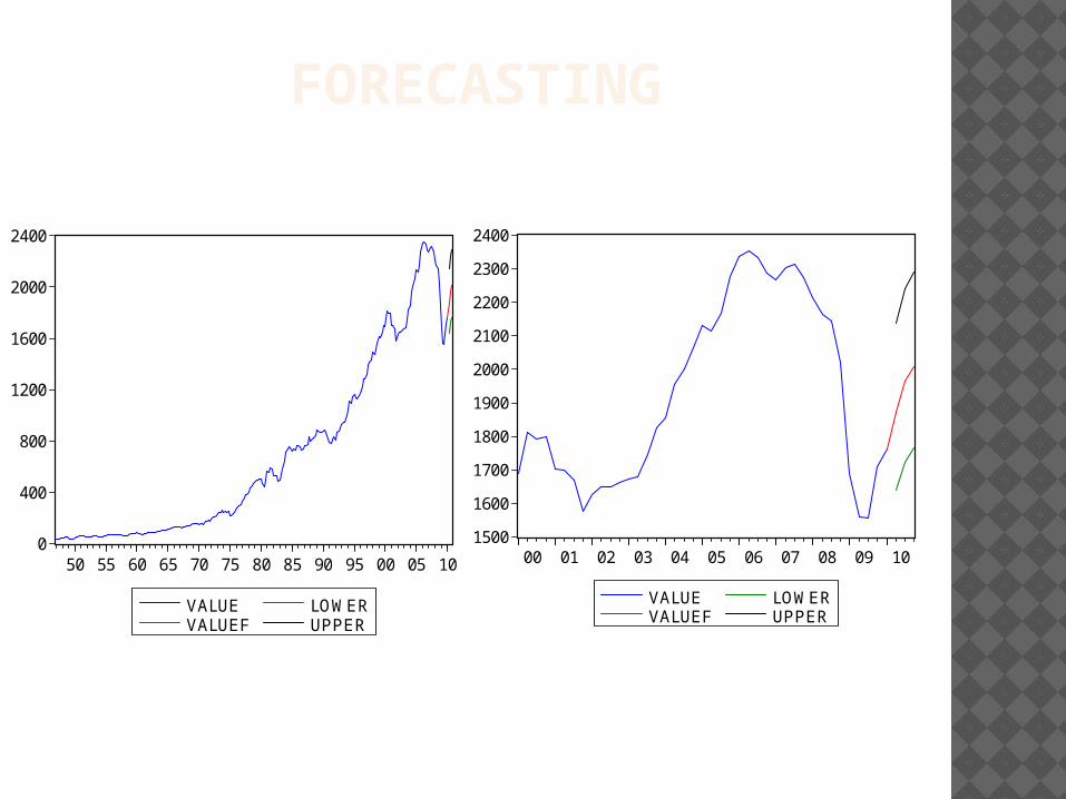
FORECASTING

0

400

800

1200

1600

2000

2400

50 55 60 65 70 75 80 85 90 95 00 05 10

VALUEVALUEF

LOWERUPPER

1500

1600

1700

1800

1900

2000

2100

2200

2300

2400

00 01 02 03 04 05 06 07 08 09 10

VALUEVALUEF

LOWERUPPER

The GDPI is increasing.It is signaling the US economy is recovering.