World-Wide Data Available for Single-Station Sigma

and

Regional Variations in the φS2S Term

Southwestern U.S. Ground Motion Characterization

SSHAC Level 3 Workshop 1 – Critical Issues and Data Needs

Adrian Rodriguez-Marek Virginia Tech

March 19-21, 2013 Oakland, CA

Outline

• Objectives

• Notation

• Available data and models

• Requirements for use of single-station sigma

2

TI Team Questions

1) What are the world-wide data (non NGA-West2) available for single-station sigma?

2) Regional variation of the fS2S term

3

Notation

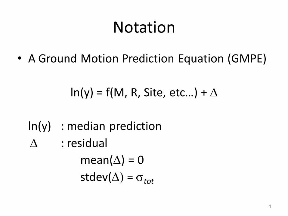
• A Ground Motion Prediction Equation (GMPE)

ln(y) = f(M, R, Site, etc…) + D

ln(y) : median prediction

D : residual

mean(D) = 0

stdev(D) = stot

4

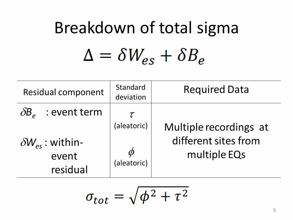
Breakdown of total sigma

Residual component Standard deviation

Required Data

dBe : event term

t (aleatoric) Multiple recordings at

different sites from multiple EQs

dWes : within-event residual

f (aleatoric)

5

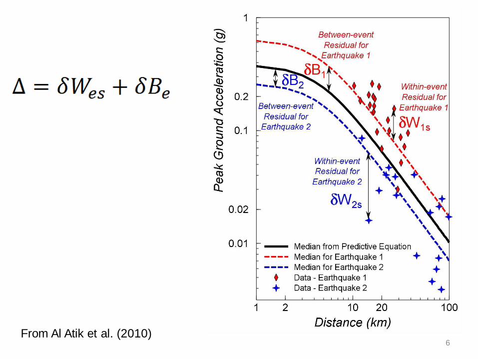
6 From Al Atik et al. (2010)

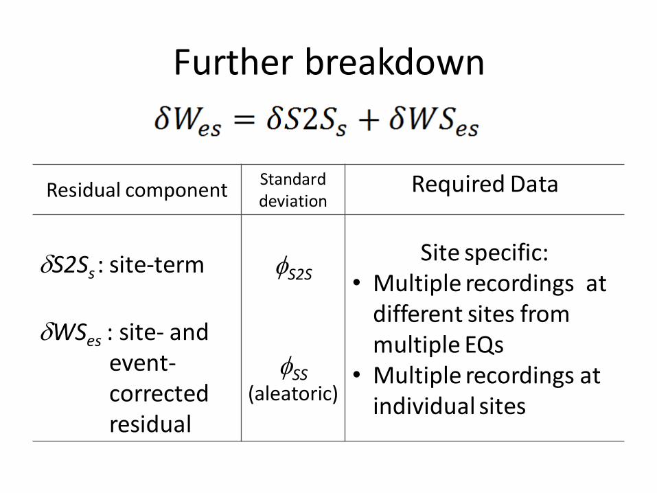
Further breakdown

Residual component Standard deviation

Required Data

dS2Ss : site-term fS2S Site specific:

• Multiple recordings at different sites from multiple EQs

• Multiple recordings at individual sites

dWSes : site- and event-corrected residual

fSS (aleatoric)

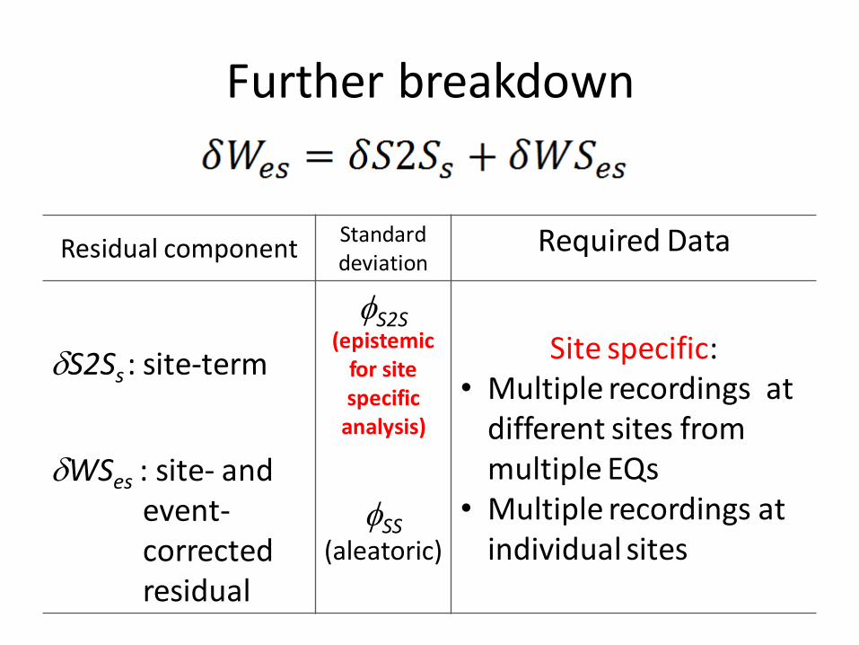
Further breakdown

Residual component Standard deviation

Required Data

dS2Ss : site-term

fS2S (epistemic

for site specific

analysis)

Site specific: • Multiple recordings at

different sites from multiple EQs

• Multiple recordings at individual sites

dWSes : site- and event-corrected residual

fSS (aleatoric)

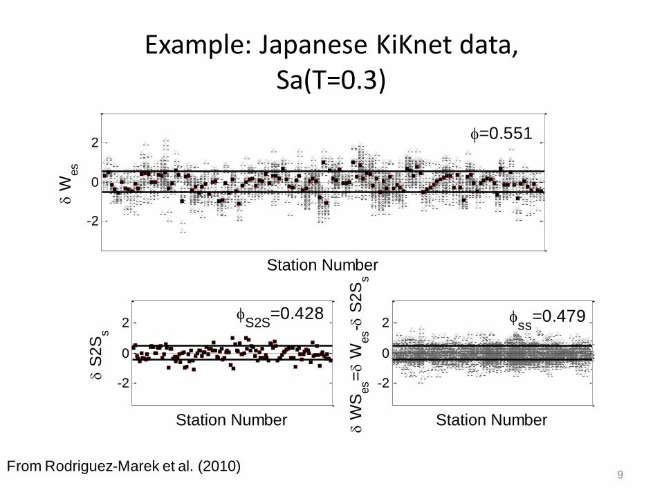
Example: Japanese KiKnet data, Sa(T=0.3)

9 From Rodriguez-Marek et al. (2010)

-2

0

2

Station Number

d W

es

f=0.551

-2

0

2

Station Number

d S

2S

s

fS2S

=0.428

-2

0

2

Station Number

d W

Ses=

d W

es-d

S2S

s

fss

=0.479

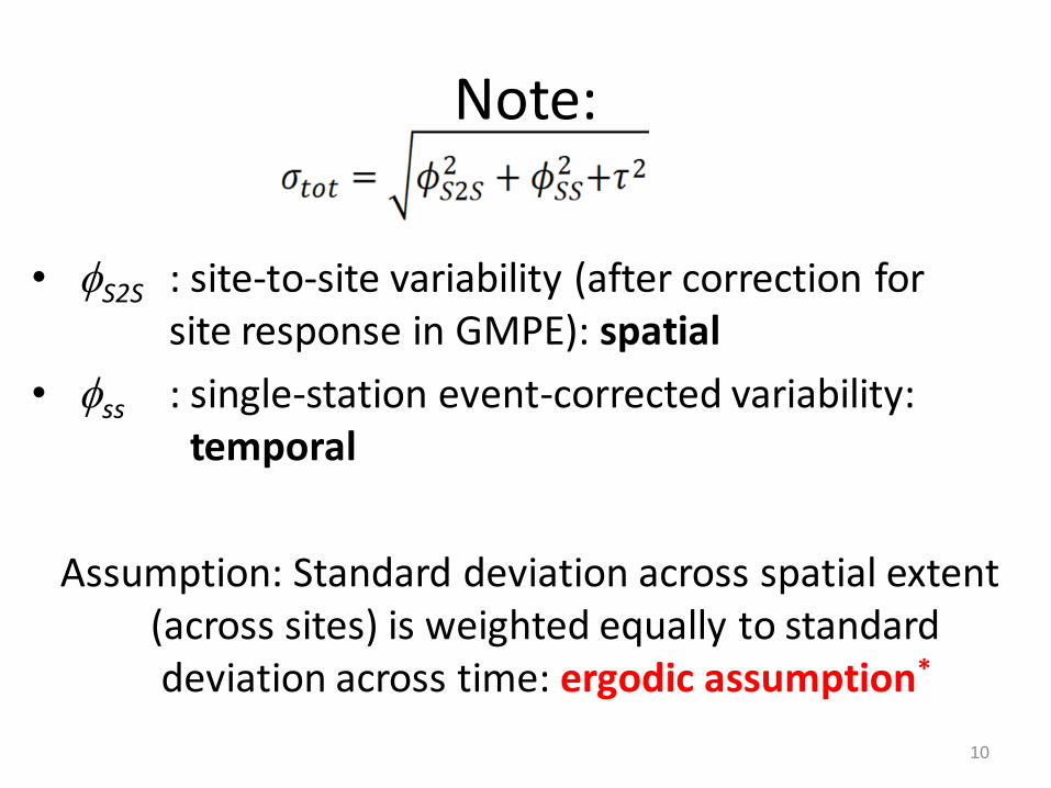
Note:

• fS2S : site-to-site variability (after correction for site response in GMPE): spatial

• fss : single-station event-corrected variability: temporal

Assumption: Standard deviation across spatial extent (across sites) is weighted equally to standard deviation across time: ergodic assumption*

10

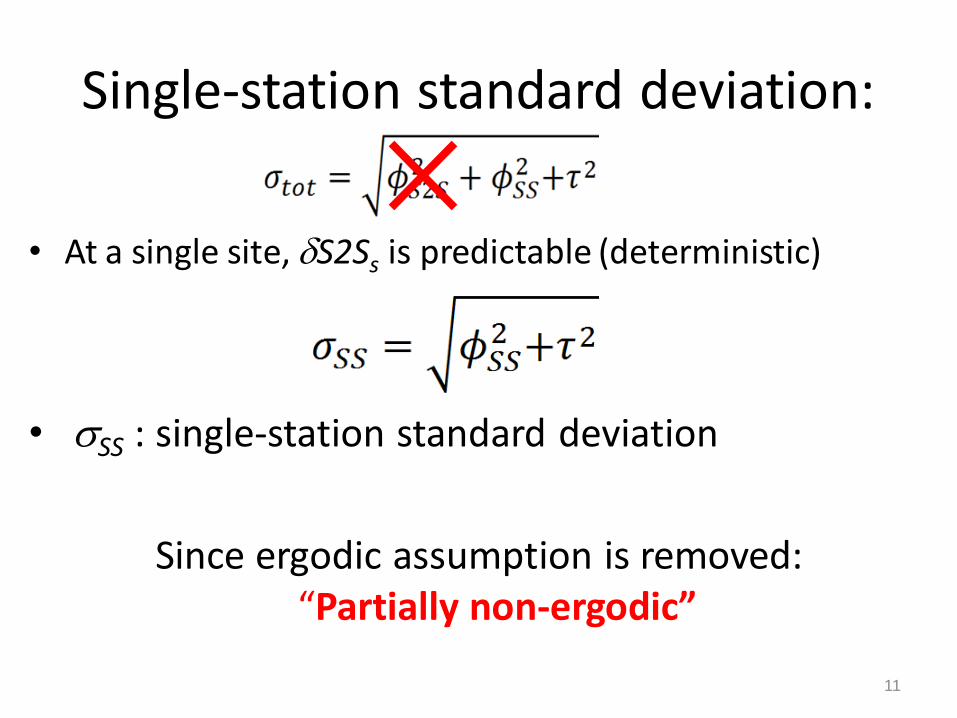
Single-station standard deviation:

• At a single site, dS2Ss is predictable (deterministic)

• sSS : single-station standard deviation

Since ergodic assumption is removed: “Partially non-ergodic”

11

MOTIVATION FOR USE OF SINGLE-STATION SIGMA

12

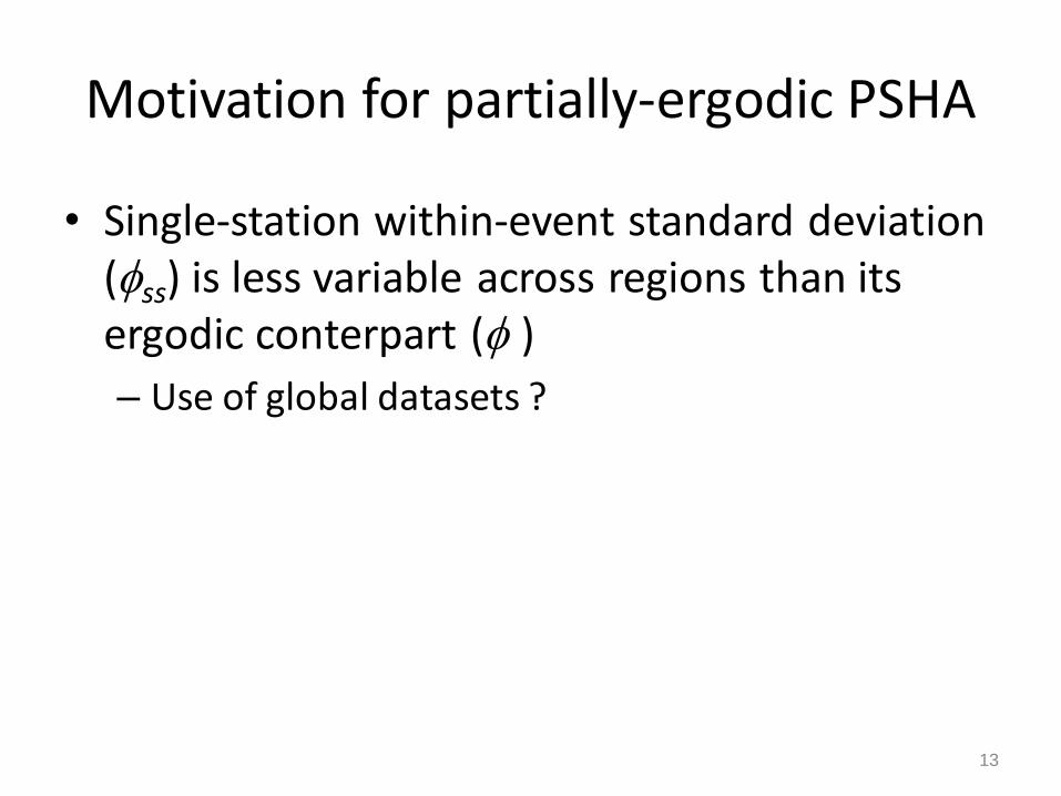
Motivation for partially-ergodic PSHA

• Single-station within-event standard deviation (fss) is less variable across regions than its ergodic conterpart (f )

– Use of global datasets ?

13

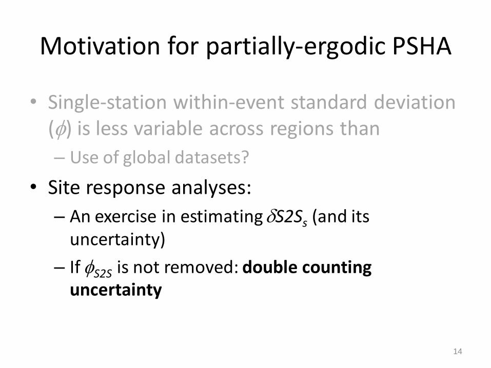
Motivation for partially-ergodic PSHA

• Single-station within-event standard deviation (f) is less variable across regions than

– Use of global datasets?

• Site response analyses:

– An exercise in estimating dS2Ss (and its uncertainty)

– If fS2S is not removed: double counting uncertainty

14

AVAILABLE DATA AND MODELS

15

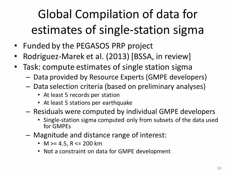
Global Compilation of data for estimates of single-station sigma

• Funded by the PEGASOS PRP project • Rodriguez-Marek et al. (2013) [BSSA, in review] • Task: compute estimates of single station sigma

– Data provided by Resource Experts (GMPE developers) – Data selection criteria (based on preliminary analyses)

• At least 5 records per station • At least 5 stations per earthquake

– Residuals were computed by individual GMPE developers • Single-station sigma computed only from subsets of the data used

for GMPEs

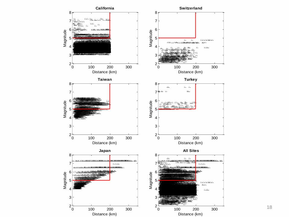
– Magnitude and distance range of interest: • M >= 4.5, R <= 200 km • Not a constraint on data for GMPE development

16

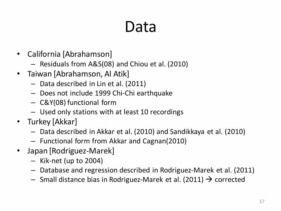
Data

• California [Abrahamson] – Residuals from A&S(08) and Chiou et al. (2010)

• Taiwan [Abrahamson, Al Atik] – Data described in Lin et al. (2011) – Does not include 1999 Chi-Chi earthquake – C&Y(08) functional form – Used only stations with at least 10 recordings

• Turkey [Akkar] – Data described in Akkar et al. (2010) and Sandikkaya et al. (2010) – Functional form from Akkar and Cagnan(2010)

• Japan [Rodriguez-Marek] – Kik-net (up to 2004) – Database and regression described in Rodriguez-Marek et al. (2011) – Small distance bias in Rodriguez-Marek et al. (2011) corrected

17

18

0 100 200 3002

3

4

5

6

7

8California

Distance (km)

Magnitude

0 100 200 3002

3

4

5

6

7

8Switzerland

Distance (km)

Magnitude

0 100 200 3002

3

4

5

6

7

8Taiwan

Distance (km)

Magnitude

0 100 200 3002

3

4

5

6

7

8Turkey

Distance (km)

Magnitude

0 100 200 3002

3

4

5

6

7

8Japan

Distance (km)

Magnitude

0 100 200 3002

3

4

5

6

7

8All Sites

Distance (km)

Magnitude

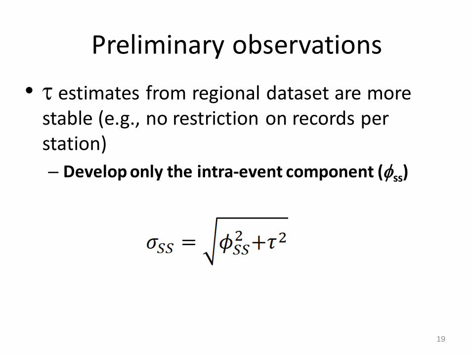
Preliminary observations

• t estimates from regional dataset are more stable (e.g., no restriction on records per station)

– Develop only the intra-event component (fss)

19

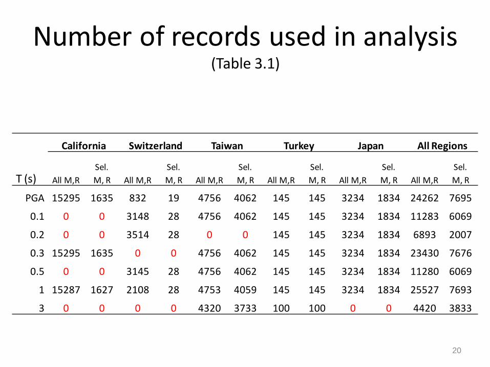
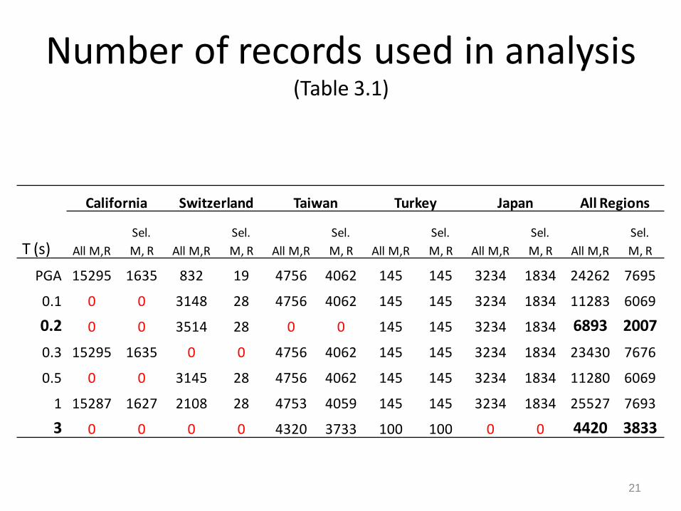
Number of records used in analysis

(Table 3.1)

20

California Switzerland Taiwan Turkey Japan All Regions

T (s) All M,R

Sel.

M, R All M,R

Sel.

M, R All M,R

Sel.

M, R All M,R

Sel.

M, R All M,R

Sel.

M, R All M,R

Sel.

M, R

PGA 15295 1635 832 19 4756 4062 145 145 3234 1834 24262 7695

0.1 0 0 3148 28 4756 4062 145 145 3234 1834 11283 6069

0.2 0 0 3514 28 0 0 145 145 3234 1834 6893 2007

0.3 15295 1635 0 0 4756 4062 145 145 3234 1834 23430 7676

0.5 0 0 3145 28 4756 4062 145 145 3234 1834 11280 6069

1 15287 1627 2108 28 4753 4059 145 145 3234 1834 25527 7693

3 0 0 0 0 4320 3733 100 100 0 0 4420 3833

Number of records used in analysis

(Table 3.1)

21

California Switzerland Taiwan Turkey Japan All Regions

T (s) All M,R

Sel.

M, R All M,R

Sel.

M, R All M,R

Sel.

M, R All M,R

Sel.

M, R All M,R

Sel.

M, R All M,R

Sel.

M, R

PGA 15295 1635 832 19 4756 4062 145 145 3234 1834 24262 7695

0.1 0 0 3148 28 4756 4062 145 145 3234 1834 11283 6069

0.2 0 0 3514 28 0 0 145 145 3234 1834 6893 2007

0.3 15295 1635 0 0 4756 4062 145 145 3234 1834 23430 7676

0.5 0 0 3145 28 4756 4062 145 145 3234 1834 11280 6069

1 15287 1627 2108 28 4753 4059 145 145 3234 1834 25527 7693

3 0 0 0 0 4320 3733 100 100 0 0 4420 3833

AVAILABLE DATA AND MODELS: GENERAL OBSERVATIONS ON GLOBAL DATABASE

23

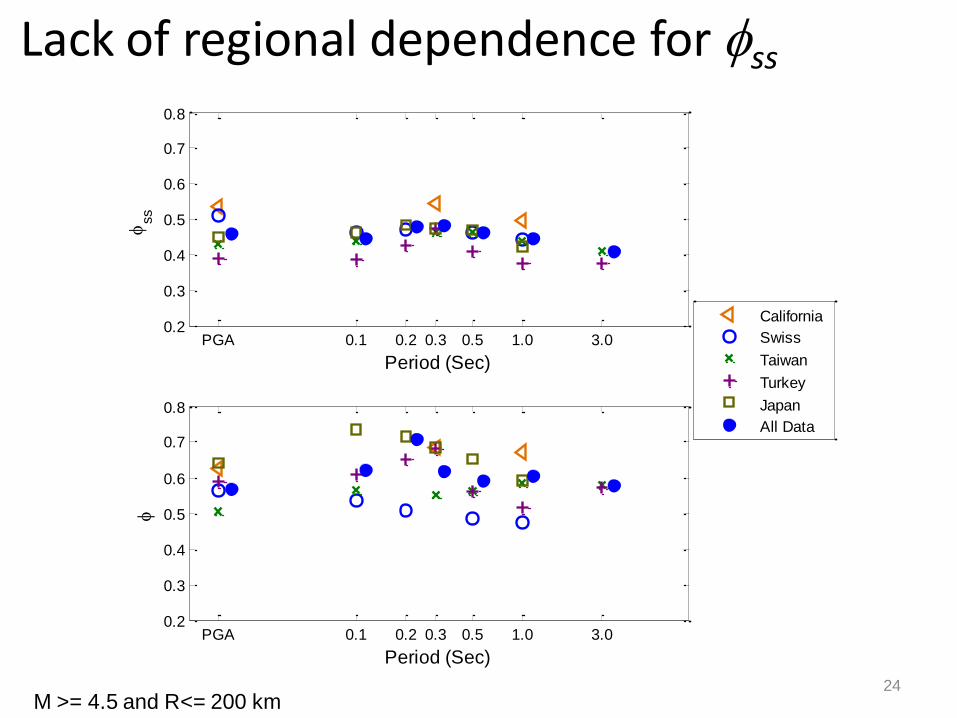
Lack of regional dependence for fss

24 M >= 4.5 and R<= 200 km

PGA 0.1 0.2 0.3 0.5 1.0 3.00.2

0.3

0.4

0.5

0.6

0.7

0.8

Period (Sec)

fss

PGA 0.1 0.2 0.3 0.5 1.0 3.00.2

0.3

0.4

0.5

0.6

0.7

0.8

Period (Sec)

f

California

Swiss

Taiwan

Turkey

Japan

All Data

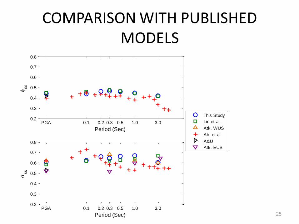
COMPARISON WITH PUBLISHED MODELS

25

This Study

Lin et al.

Atk. WUS

Ab. et al.

A&U

Atk. EUS

PGA 0.1 0.2 0.3 0.5 1.0 3.00.2

0.3

0.4

0.5

0.6

0.7

0.8

Period (Sec)

fss

PGA 0.1 0.2 0.3 0.5 1.0 3.00.2

0.3

0.4

0.5

0.6

0.7

0.8

Period (Sec)

sss

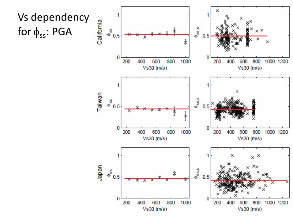
Vs dependency for fss: PGA

27

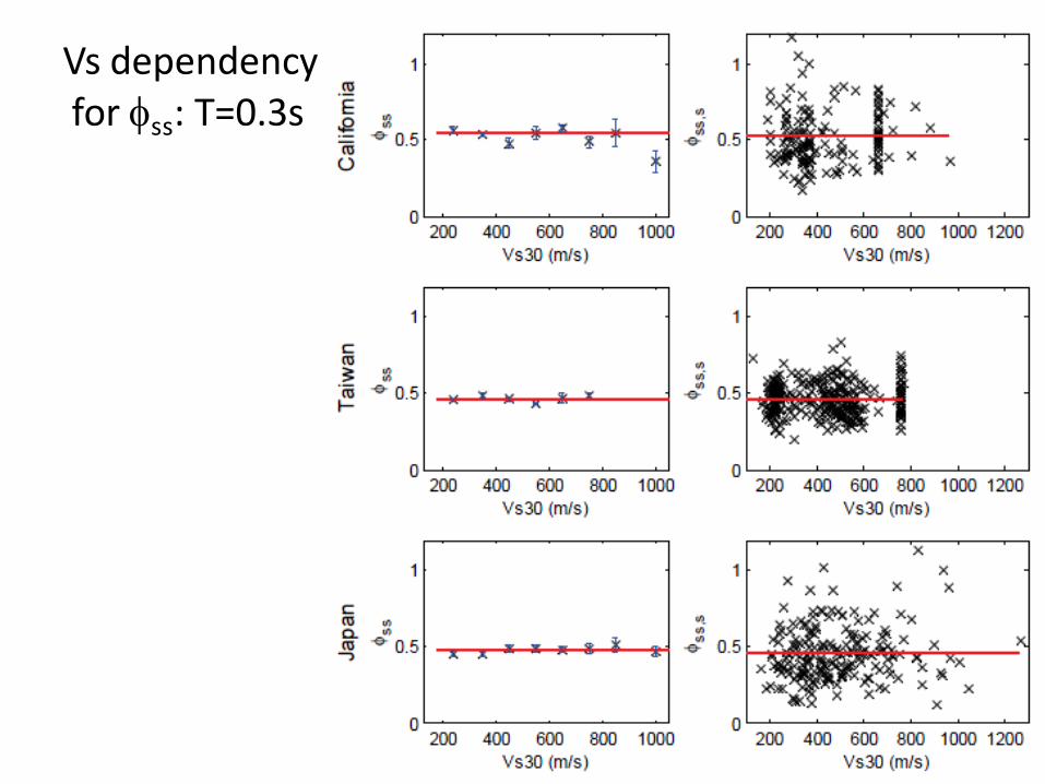
Vs dependency for fss: T=0.3s

28

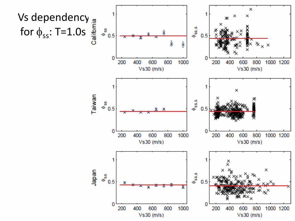
Vs dependency for fss: T=1.0s

29

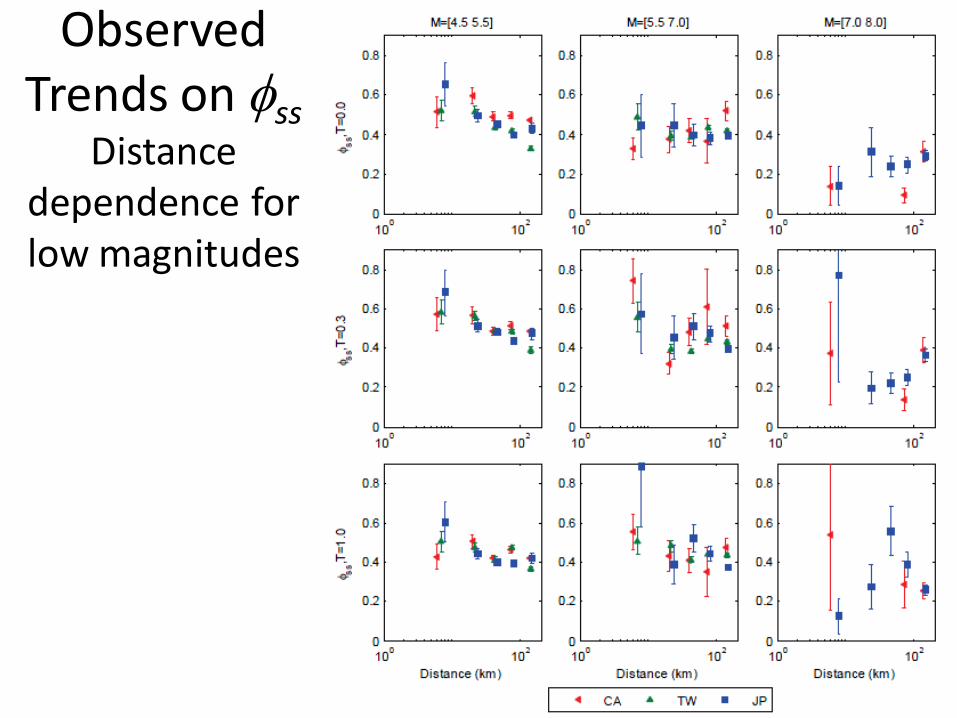
Observed Trends on fss

Distance dependence for low magnitudes

30

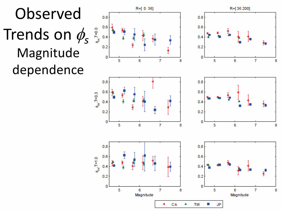
Observed Trends on fss

Magnitude dependence

31

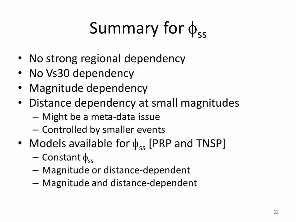
Summary for fss

• No strong regional dependency • No Vs30 dependency • Magnitude dependency • Distance dependency at small magnitudes

– Might be a meta-data issue – Controlled by smaller events

• Models available for fss [PRP and TNSP] – Constant fss

– Magnitude or distance-dependent – Magnitude and distance-dependent

32

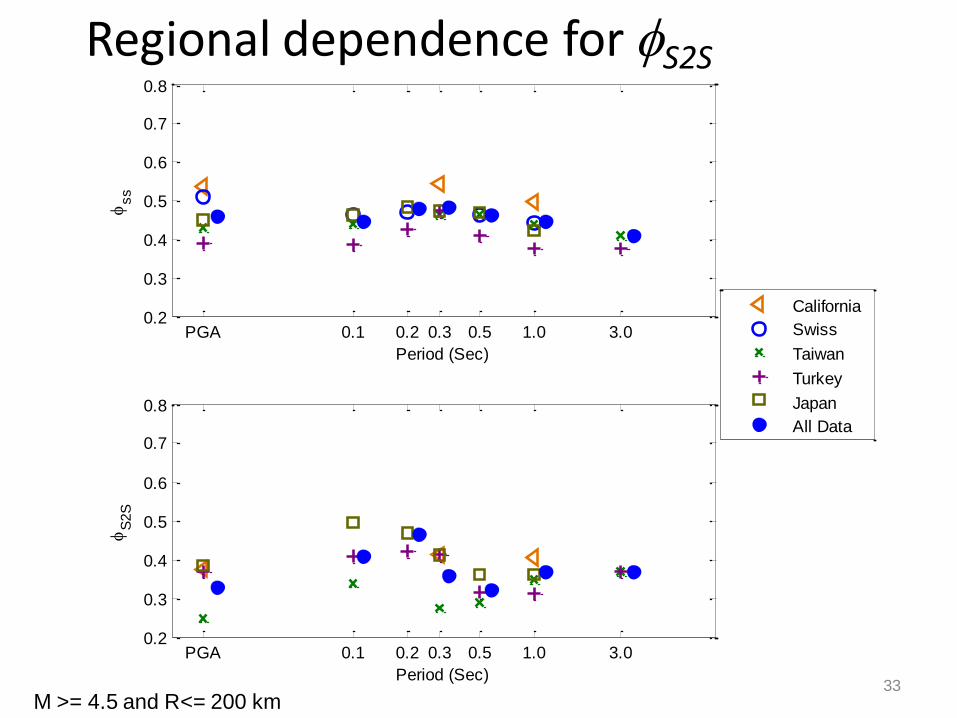
Regional dependence for fS2S

33 M >= 4.5 and R<= 200 km

PGA 0.1 0.2 0.3 0.5 1.0 3.00.2

0.3

0.4

0.5

0.6

0.7

0.8

Period (Sec)

fss

PGA 0.1 0.2 0.3 0.5 1.0 3.00.2

0.3

0.4

0.5

0.6

0.7

0.8

Period (Sec)

fS

2S

California

Swiss

Taiwan

Turkey

Japan

All Data

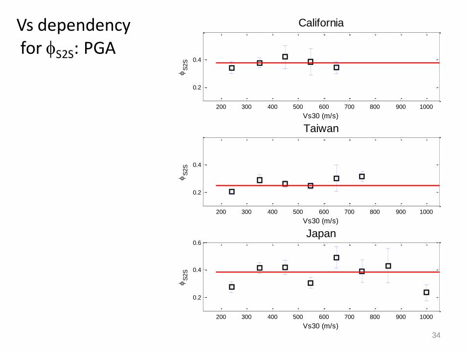
Vs dependency for fS2S: PGA

34

200 300 400 500 600 700 800 900 1000

0.2

0.4

Vs30 (m/s)

fS

2S

California

200 300 400 500 600 700 800 900 1000

0.2

0.4

Vs30 (m/s)

fS

2S

Taiwan

200 300 400 500 600 700 800 900 1000

0.2

0.4

0.6

Vs30 (m/s)

fS

2S

Japan

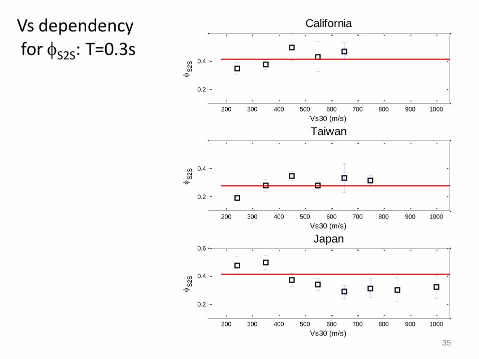
Vs dependency for fS2S: T=0.3s

35

200 300 400 500 600 700 800 900 1000

0.2

0.4

Vs30 (m/s)

fS

2S

California

200 300 400 500 600 700 800 900 1000

0.2

0.4

Vs30 (m/s)

fS

2S

Taiwan

200 300 400 500 600 700 800 900 1000

0.2

0.4

0.6

Vs30 (m/s)

fS

2S

Japan

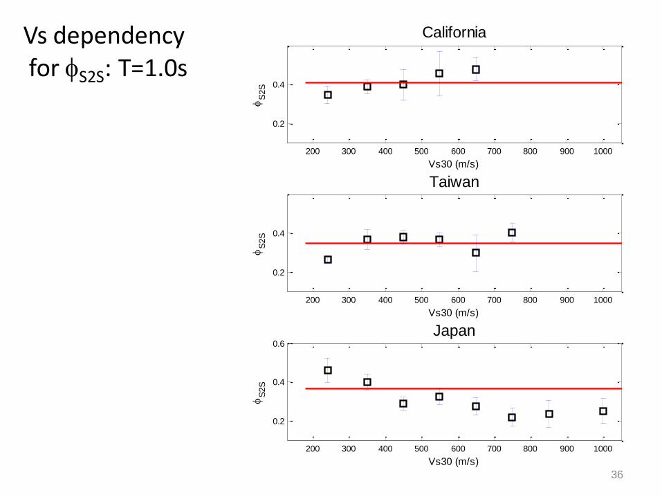
Vs dependency for fS2S: T=1.0s

36

200 300 400 500 600 700 800 900 1000

0.2

0.4

Vs30 (m/s)

fS

2S

California

200 300 400 500 600 700 800 900 1000

0.2

0.4

Vs30 (m/s)

fS

2S

Taiwan

200 300 400 500 600 700 800 900 1000

0.2

0.4

0.6

Vs30 (m/s)

fS

2S

Japan

Summary for fS2S

• Stronger regional dependency than fss

• There might be Vs30 dependency in some datasets

37

REQUIREMENTS FOR USE OF SINGLE-STATION SIGMA

38

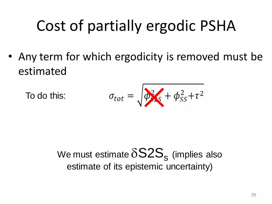
Cost of partially ergodic PSHA

• Any term for which ergodicity is removed must be estimated

39

To do this:

We must estimate dS2Ss (implies also

estimate of its epistemic uncertainty)

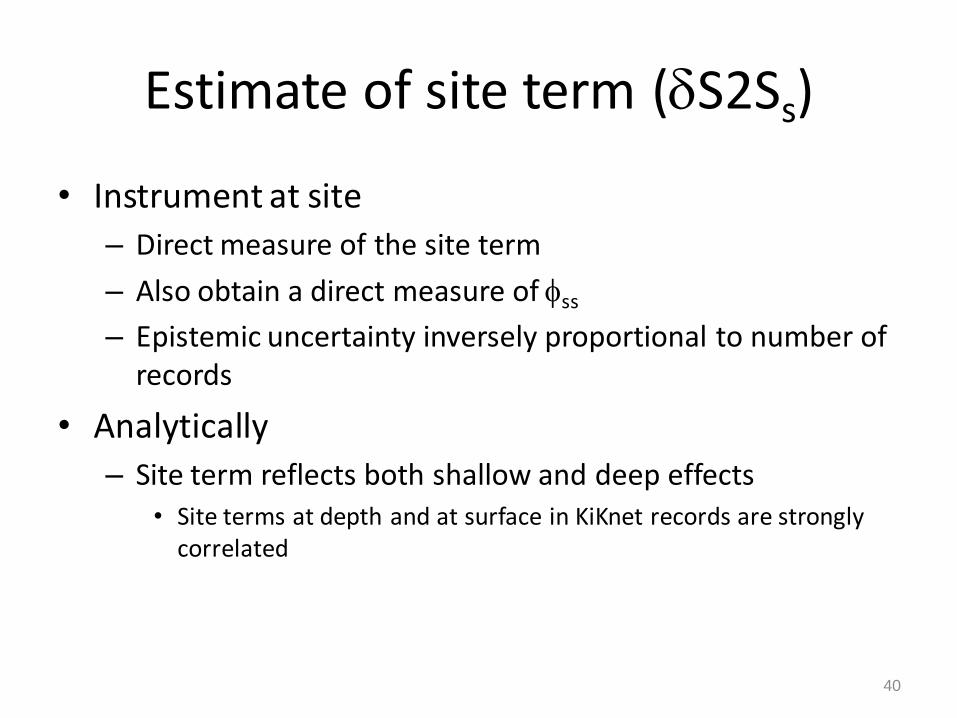
Estimate of site term (dS2Ss)

• Instrument at site

– Direct measure of the site term

– Also obtain a direct measure of fss

– Epistemic uncertainty inversely proportional to number of records

• Analytically

– Site term reflects both shallow and deep effects • Site terms at depth and at surface in KiKnet records are strongly

correlated

40

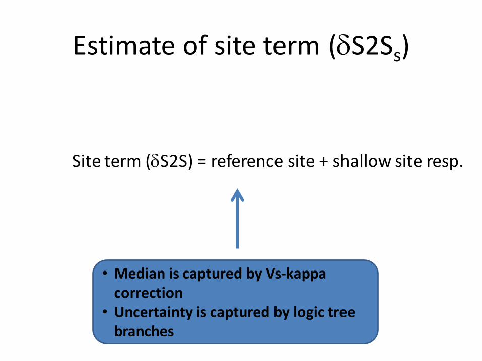
Estimate of site term (dS2Ss)

Site term (dS2S) = reference site + shallow site resp.

• Median is captured by Vs-kappa correction

• Uncertainty is captured by logic tree branches

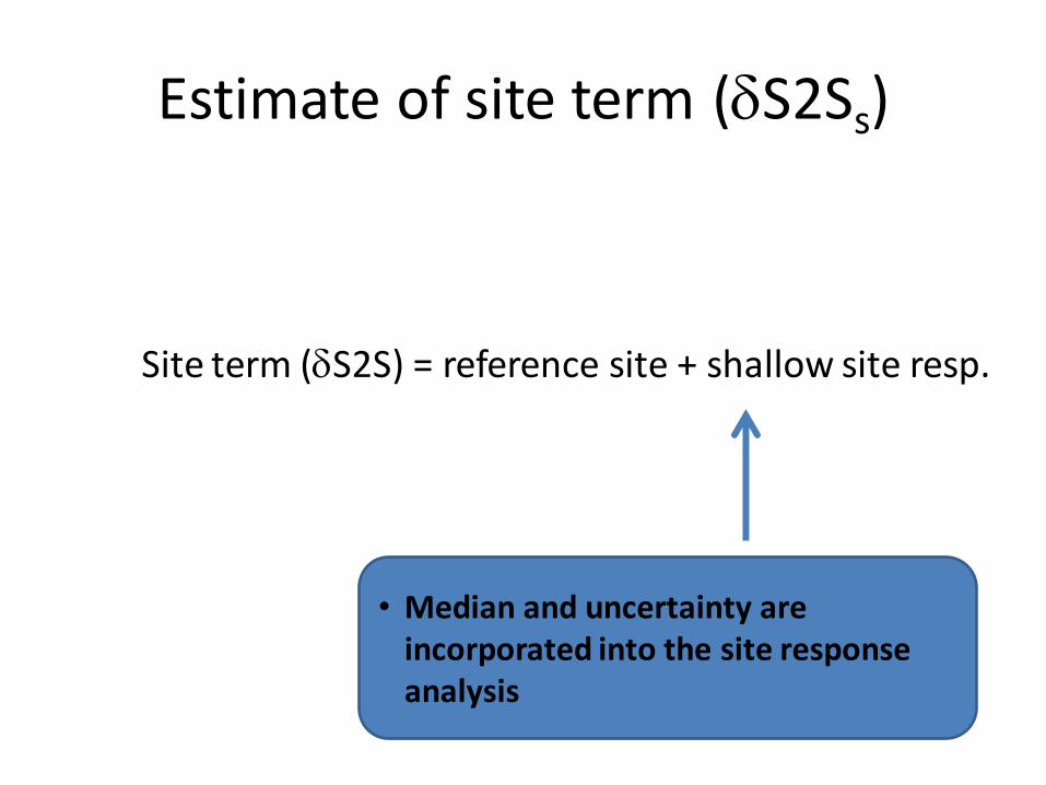
Estimate of site term (dS2Ss)

Site term (dS2S) = reference site + shallow site resp.

• Median and uncertainty are incorporated into the site response analysis

Uncertainty in fss

• Both the site term (dS2Ss) and the single-station standard deviation (fss) have epistemic uncertainties.

– Different stations sample different sources/paths

– 2D and 3D effects imply azimuthal dependency

– Degree of nonlinearity

43

Summary of requirements for using single-station sigma

• Site term (dS2S) must be estimated

• Epistemic uncertainty on site term must be estimated and accounted for

• Epistemic uncertainty on fss must be accounted for

44

VARIATION OF fss FROM STATION TO STATION

45

Epistemic uncertainty on fss

• Both the site term (dS2Ss) and the single-station standard deviation (fss) have epistemic uncertainties.

– Different stations sample different sources/paths

– 2D and 3D effects imply azimuthal dependency

– Degree of nonlinearity

46

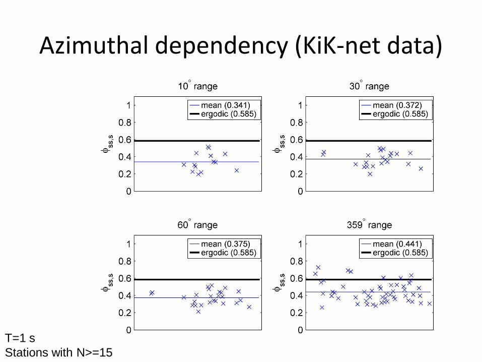
Azimuthal dependency (KiK-net data)

47 T=1 s Stations with N>=15

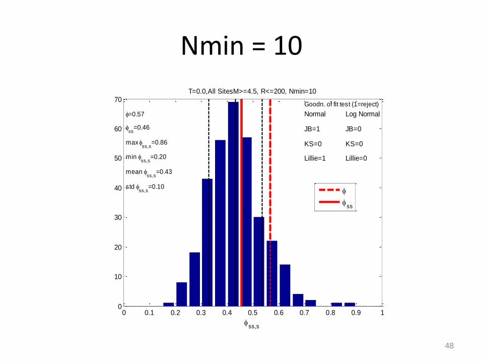
Nmin = 10

48

0 0.1 0.2 0.3 0.4 0.5 0.6 0.7 0.8 0.9 10

10

20

30

40

50

60

70Goodn. of fit test (1=reject)

Normal

JB=1

KS=0

Lillie=1

Log Normal

JB=0

KS=0

Lillie=0

f=0.57

fss

=0.46

max fss,s

=0.86

min fss,s

=0.20

mean fss,s

=0.43

std fss,s

=0.10

T=0.0,All SitesM>=4.5, R<=200, Nmin=10

fss,s

f

fss

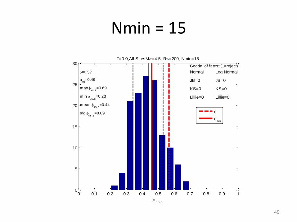
Nmin = 15

49

0 0.1 0.2 0.3 0.4 0.5 0.6 0.7 0.8 0.9 10

5

10

15

20

25

30Goodn. of fit test (1=reject)

Normal

JB=0

KS=0

Lillie=0

Log Normal

JB=0

KS=0

Lillie=0

f=0.57

fss

=0.46

max fss,s

=0.69

min fss,s

=0.23

mean fss,s

=0.44

std fss,s

=0.09

T=0.0,All SitesM>=4.5, R<=200, Nmin=15

fss,s

f

fss

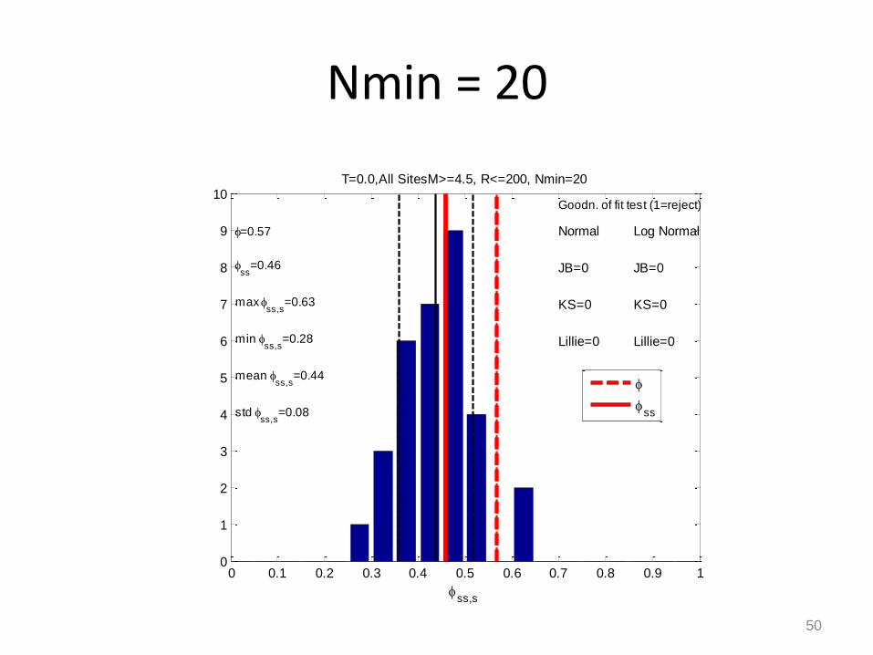
Nmin = 20

50

0 0.1 0.2 0.3 0.4 0.5 0.6 0.7 0.8 0.9 10

1

2

3

4

5

6

7

8

9

10Goodn. of fit test (1=reject)

Normal

JB=0

KS=0

Lillie=0

Log Normal

JB=0

KS=0

Lillie=0

f=0.57

fss

=0.46

max fss,s

=0.63

min fss,s

=0.28

mean fss,s

=0.44

std fss,s

=0.08

T=0.0,All SitesM>=4.5, R<=200, Nmin=20

fss,s

f

fss

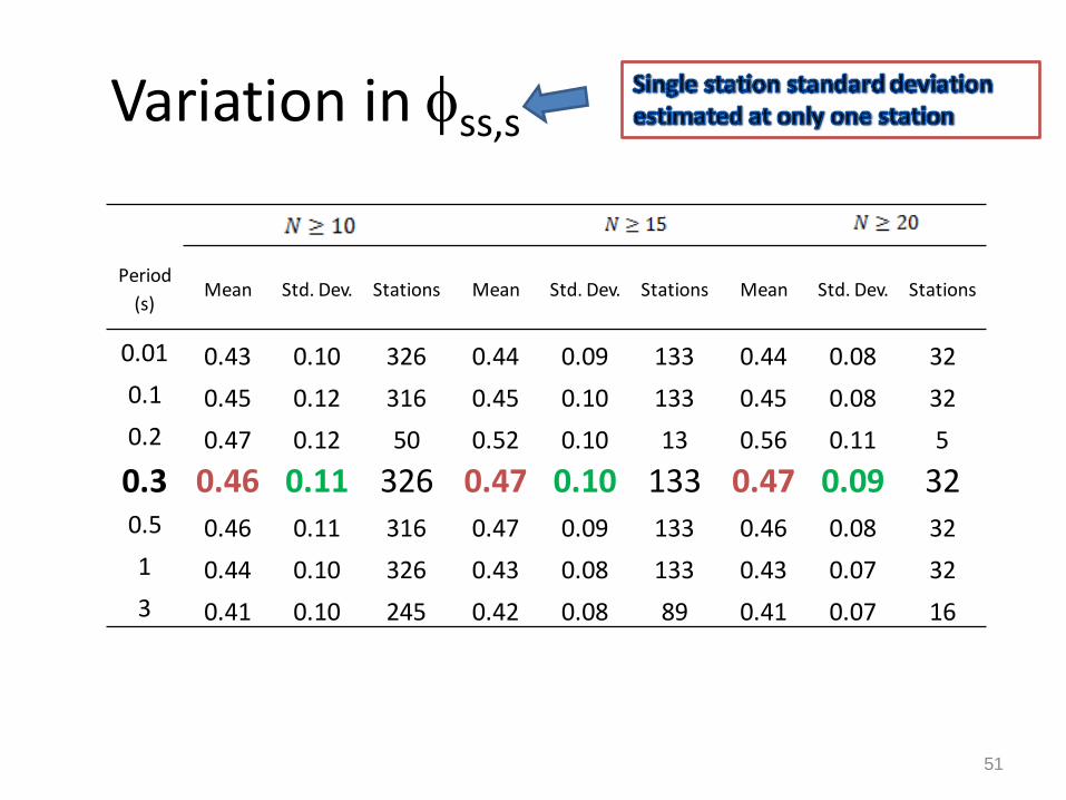
Variation in fss,s

51

Period

(s) Mean Std. Dev. Stations Mean Std. Dev. Stations Mean Std. Dev. Stations

0.01 0.43 0.10 326 0.44 0.09 133 0.44 0.08 32

0.1 0.45 0.12 316 0.45 0.10 133 0.45 0.08 32

0.2 0.47 0.12 50 0.52 0.10 13 0.56 0.11 5

0.3 0.46 0.11 326 0.47 0.10 133 0.47 0.09 32 0.5 0.46 0.11 316 0.47 0.09 133 0.46 0.08 32

1 0.44 0.10 326 0.43 0.08 133 0.43 0.07 32

3 0.41 0.10 245 0.42 0.08 89 0.41 0.07 16

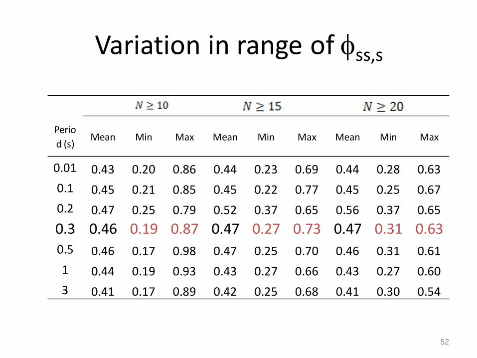
Variation in range of fss,s

52

Perio

d (s) Mean Min Max Mean Min Max Mean Min Max

0.01 0.43 0.20 0.86 0.44 0.23 0.69 0.44 0.28 0.63

0.1 0.45 0.21 0.85 0.45 0.22 0.77 0.45 0.25 0.67

0.2 0.47 0.25 0.79 0.52 0.37 0.65 0.56 0.37 0.65

0.3 0.46 0.19 0.87 0.47 0.27 0.73 0.47 0.31 0.63 0.5 0.46 0.17 0.98 0.47 0.25 0.70 0.46 0.31 0.61

1 0.44 0.19 0.93 0.43 0.27 0.66 0.43 0.27 0.60

3 0.41 0.17 0.89 0.42 0.25 0.68 0.41 0.30 0.54

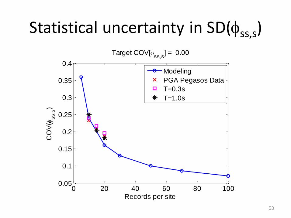
Statistical uncertainty in SD(fss,s)

53

0 20 40 60 80 1000.05

0.1

0.15

0.2

0.25

0.3

0.35

0.4

Target COV[fss,s

] = 0.00

Records per site

CO

V(f

ss,s

)

Modeling

PGA Pegasos Data

T=0.3s

T=1.0s

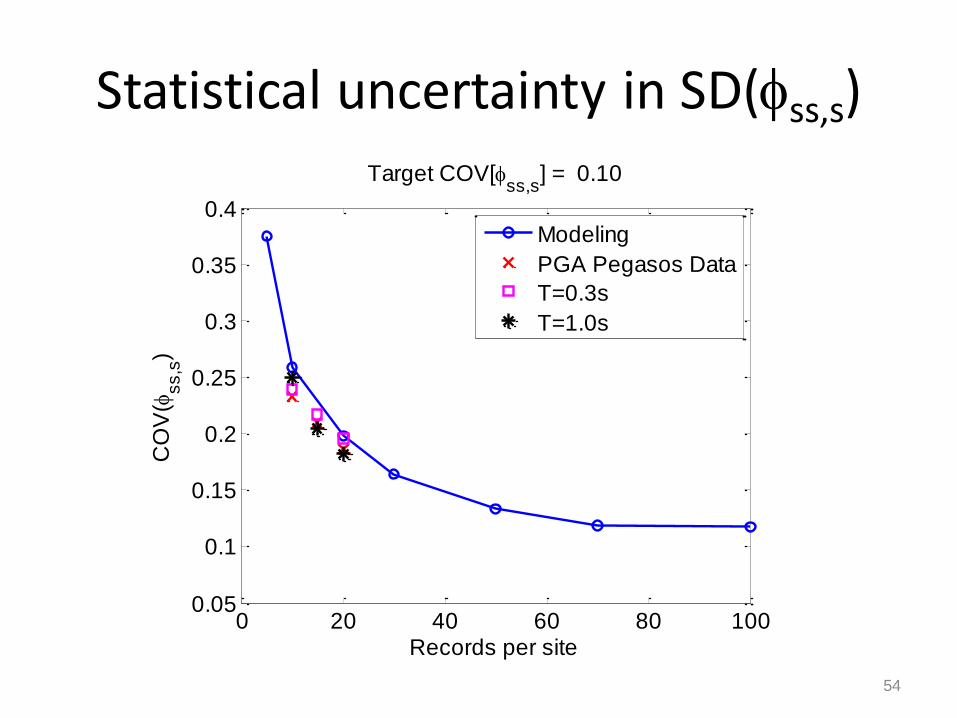
0 20 40 60 80 1000.05

0.1

0.15

0.2

0.25

0.3

0.35

0.4

Target COV[fss,s

] = 0.10

Records per site

CO

V(f

ss,s

)

Modeling

PGA Pegasos Data

T=0.3s

T=1.0s

Statistical uncertainty in SD(fss,s)

54

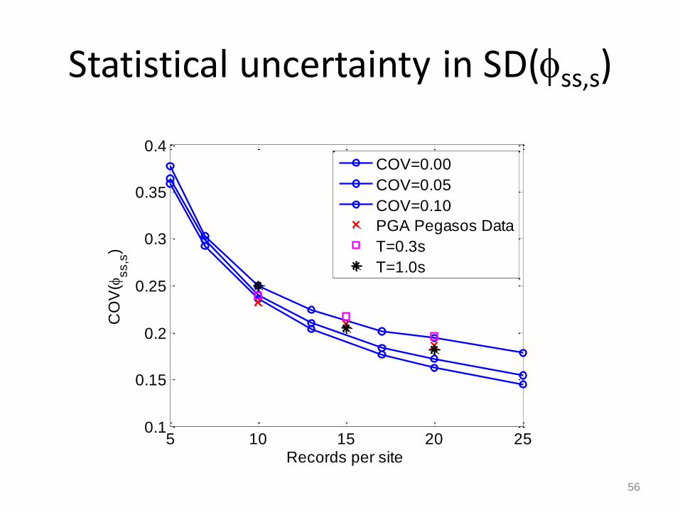
Statistical uncertainty in SD(fss,s)

56

5 10 15 20 250.1

0.15

0.2

0.25

0.3

0.35

0.4

Records per site

CO

V(f

ss,s

)

COV=0.00

COV=0.05

COV=0.10

PGA Pegasos Data

T=0.3s

T=1.0s

Epistemic Uncertainty on fss

Summary

• The standard deviation of the single-station phi measured at each station [std(fss,s)] can be used as a basis to assign epistemic uncertainty on fss

– Use well recorded stations (N>20) to estimate std(fss,s)

– Use modeling to estimate pure uncertainty (e.g., uncertainty that does not include statistical uncertainty)

57

Thank you

58

California data

• The California dataset used in this study consists of ground motion data from the Abrahamson and Silva (2008) NGA dataset and small-to-moderate magnitude California data used for the small magnitude extension of the Chiou and Youngs (2008) NGA model (Chiou et al., 2010) at peak ground acceleration (PGA) and at periods of 0.3 and 1 second. The Abrahamson and Silva (2008) data are part of the NGA West dataset. The small-to-moderate magnitude data used in Chiou et al. (2010) were obtained from ShakeMap.

• Between-event residuals and within-event residuals of these two California datasets were obtained by separately fitting the large magnitude and small-to-moderate magnitude datasets with the Abrahamson and Silva (2008) GMPE and with the Chiou et al. (2010) GMPE, respectively.

59

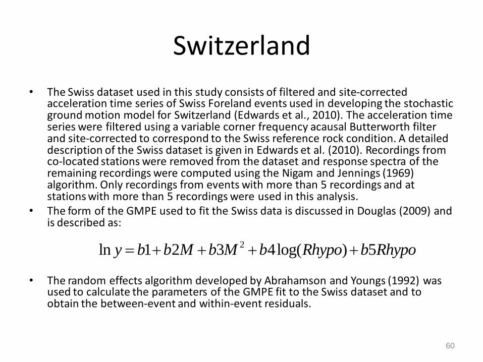
Switzerland

• The Swiss dataset used in this study consists of filtered and site-corrected acceleration time series of Swiss Foreland events used in developing the stochastic ground motion model for Switzerland (Edwards et al., 2010). The acceleration time series were filtered using a variable corner frequency acausal Butterworth filter and site-corrected to correspond to the Swiss reference rock condition. A detailed description of the Swiss dataset is given in Edwards et al. (2010). Recordings from co-located stations were removed from the dataset and response spectra of the remaining recordings were computed using the Nigam and Jennings (1969) algorithm. Only recordings from events with more than 5 recordings and at stations with more than 5 recordings were used in this analysis.

• The form of the GMPE used to fit the Swiss data is discussed in Douglas (2009) and is described as:

• The random effects algorithm developed by Abrahamson and Youngs (1992) was

used to calculate the parameters of the GMPE fit to the Swiss dataset and to obtain the between-event and within-event residuals.

60

2ln 1 2 3 4log( ) 5y b b M b M b Rhypo b Rhypo

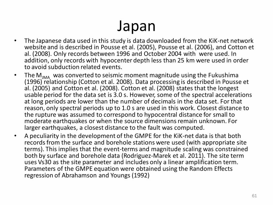
Japan • The Japanese data used in this study is data downloaded from the KiK-net network

website and is described in Pousse et al. (2005), Pousse et al. (2006), and Cotton et al. (2008). Only records between 1996 and October 2004 with were used. In addition, only records with hypocenter depth less than 25 km were used in order to avoid subduction related events.

• The MJMA was converted to seismic moment magnitude using the Fukushima (1996) relationship (Cotton et al. 2008). Data processing is described in Pousse et al. (2005) and Cotton et al. (2008). Cotton et al. (2008) states that the longest usable period for the data set is 3.0 s. However, some of the spectral accelerations at long periods are lower than the number of decimals in the data set. For that reason, only spectral periods up to 1.0 s are used in this work. Closest distance to the rupture was assumed to correspond to hypocentral distance for small to moderate earthquakes or when the source dimensions remain unknown. For larger earthquakes, a closest distance to the fault was computed.

• A peculiarity in the development of the GMPE for the KiK-net data is that both records from the surface and borehole stations were used (with appropriate site terms). This implies that the event-terms and magnitude scaling was constrained both by surface and borehole data (Rodriguez-Marek et al. 2011). The site term uses Vs30 as the site parameter and includes only a linear amplification term. Parameters of the GMPE equation were obtained using the Random Effects regression of Abrahamson and Youngs (1992)

61

Taiwan

• The Taiwan dataset used in this study consists of ground motion data from shallow earthquakes that occurred in and near Taiwan from 1992 to 2003. This dataset was assembled by Lin (2009) and the ground motion recordings were baseline corrected and limited to distances of less than 200 km. The 1999 Chi-Chi earthquake was excluded from the dataset. A more detailed description of the Taiwan data is given in Lin et al. (2011). Within-event and between-event residuals of the Taiwan dataset were computed using a mixed-effects algorithm with respect to a revised version of the Chiou and Youngs (2008) model. Only stations with at least 10 recordings were used to calculate the site terms.

62

Turkey • The Turkish data used in this study is compiled within the framework of the project entitled

“Compilation of Turkish strong-motion network according to the international standards.” The procedures followed to assemble the database are described in Akkar et al. (2010) and Sandıkkaya et al. (2010). The dataset comprises of events with depths less than 30 km. Each event in the dataset has at least 5 recordings. The distance measure is Joyner-Boore distance metric for all recordings. For small events (i.e., Mw 5.5) epicentral distance is assumed to approximate Joyner-Boore distance. The dataset is processed (band-pass acausal filtering) by the method described in Akkar and Bommer (2006). The same article also describes a set of criteria for computing the usable spectral period range that is used to define the maximum usable period for each processed record. The database consists of very few recordings with VS30 > 760 m/s (where Vs30 is the average shear wave velocity over the upper 30 m of a profile) and almost all events are either strike-slip or normal. The database contains 239 recordings but this number is reduced to 206 at T = 3.0 s due usable period range criteria in Akkar and Bommer (2006).

• Regression analysis is conducted using the above dataset to derive a set of GMPEs for the analysis of within event residuals. A one-stage maximum likelihood regression method (Joyner and Boore, 1993) is employed while developing the GMPEs. The model estimates the geometric mean of the ground motion. The functional form is the same one that is presented in Akkar and Çağnan (2010). It is capable of capturing magnitude saturation and magnitude-dependent geometrical spreading. Site effects are considered using a function of Vs30 that also includes nonlinearity.

63

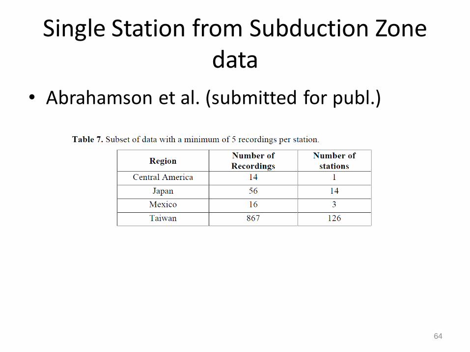
Single Station from Subduction Zone data

• Abrahamson et al. (submitted for publ.)

64

References • Abrahamson, N.A. & W.J. Silva (2008). Summary of the Abrahamson & Silva NGA ground-motion relations.

Earthquake Spectra 24(1), 67-97. • Abrahamson, N.A. & W.J. Silva (2009). Errata for ‘Summary of the Abrahamson & Silva NGA ground-motion

relations’. PEER NGA website • Abrahamson, N.A., Gregor, N., and Addo, K. (2012). “BCHydro ground motion prediction equations for

subduction earthquakes,” Submitted to Earthquake Spectra. • Akkar, S., and Z. Çagnan (2010). A Local Ground-Motion Predictive Model for Turkey, and Its Comparison

with Other Regional and Global Ground-Motion Models, Bull. Seismol. Soc. Am. 100, 2978-2995. • Al-Atik, L., N. Abrahamson, F. Cotton, F. Scherbaum, J. Bommer, and N. Kuehn (2010). The variability of

ground-motion prediction models and its components, Seismol. Res. Lett. 81, no. 5, 794–801. • Anderson, J. G. and J. N. Brune (1999). Probabilistic seismic hazard assessment without the ergodic

assumption, Seism. Res. Let., 70, 19-28. • Anderson, J.G., and Uchiyama (2011). “A Methodology to Improve Ground Motion Prediction Equations by

Including Path Corrections .” Accepted for Publication, BSSA. • Atkinson, G. M. (2006). Single-station sigma, Bull. Seism. Soc. Am., 96, 446-455. • Bommer, J. J., and N. A. Abrahamson (2006). Why do modern probabilistic seismic-hazard analyses often

lead to increased hazard estimates?, Bull. Seismol. Soc. Am. 96 1967–1977. • Chiou, B.S.J & R.R. Youngs (2008). An NGA model for the average horizontal component of peak ground

motion and response spectra. Earthquake Spectra 24(1), 173-215. • Chiou, B.S.J., R.R. Youngs, N.A. Abrahamson & K. Addo (2010). Ground-motion attenuation model for small-

to-moderate shallow crustal earthquakes in California and its implications on regionalization of ground-motion prediction models. Earthquake Spectra 26(4), 907-926.

65

References

• Chen Y-H., and C-C. P. Tsai (2002). A new method for estimation of the attenuation relationship with variance components, Bull. Seism. Soc. Am., 92, 1984-1991.

• Lin, P-S., Chiou, B., Abrahamson, N., Walling, M., Lee, C-T, and Cheng, C-T (2011). “Repeatable source, site, and path effects on the standard deviation for empirical ground-motion prediction models.” Bulletin of the Seismological Society of America, 101(5), 2281-2295.

• McGuire, R.K., Silva W.J., and Costantino, C.J. (2001). “Technical basis for revision of regulatory guidance on design ground motions: Hazard- and Risk- consistent groudn motion spectra guidelines. NUREG/CR-6728.” Prepared for the USNRC, Washington DC.

• Morikawa, N., T. Kanno, A. Narita, H. Fujiwara, T. Okumura, Y. Fukushima, and A. Guerpinar (2008). Strong motion uncertainty determined from observed records by dense network in Japan, J. Seism., 12(4):529-546.

• Rodriguez-Marek, A., and F. Cotton (2011). “Draft final report: single station sigma project” Pegasos Refinement Project, report EXT-TB-1058.

• Rodriguez-Marek. A., G. A. Montalva, F. Cotton, and F. Bonilla (2011). Analysis of Single-Station Standard Deviation Using the KiK-net Data, Bull. Seismol. Soc. Am. 101 1242–1258.

• Rodriguez-Marek, A., Cotton, F., Abrahamson, N., Akkar, S., Al Atik, L., Edwards, B., Montalva, G.A., and Dawood, H.M. (2013). “A model for single-station standard deviation using data from various tectonic regions.” Submitted to BSSA, February 2013.

• Sandıkkaya, M. A., M. T. Yılmaz, B. B. Bakır, and Ö. Yılmaz (2010). Site classification of Turkish national strong-motion stations, Journal of Seismology 14, 543–563.

• Walling, M. A. (2009). Non-Ergodic Probabilistic Seismic Hazard Analysis and Simulation Spatial of Variation in Ground Motion, PhD. Thesis, University of California, Berkeley, Department of Civil and Environment Engineering.

66

EXTRA SLIDES

67