Analyzing the Factors of Deforestation in the Amazon using GIS and Logistic Regression

Maximilian Ornat, Kale Smith & Sophie Zajaczkiwsky

April 10th 2020

Professor Ben DeVries | GEOG*4480 University of Guelph

2

Abstract

Deforestation is a shockingly destructive worldwide issue silently contributing to climate

change. Unfortunately, in the Amazon, deforestation rates have been climbing since 2012, mainly due

to agriculture expansion and institutionalized issues and remiss regulations. Using a GIS-based spatial

analysis and logistic regression, this project aimed to explore different factors affecting deforestation

(roads, waterbodies, protected area and slope) and create a predictive model. Analysis was conducted

in southern Roraima, Brazil, to determine factor(s) most influential to deforestation in that location. It

was found that the only main factor influencing deforestation at this site are the roads. Conclusions

were supported by the p value for roads (p value = 9.49e-05) at a 95% confidence interval and the

Akaike Information Criterion (AIC) evaluation of four models. Through this same analysis water bodies,

protected areas and slopes were not determined to be statistically significant using spatial regression

when used to compare predicted to actual deforestation. Further analysis which was not covered in

the model included factors such as city size and land use. In addition, the application of the model to

other sites in other areas of the world was not proven effective.

3

Table of Contents

Contents Abstract ............................................................................................................................................ 2

Table of Contents ............................................................................................................................... 3

Problem Context & Purpose ............................................................................................................... 4

Problem Definition and Significance of Research ......................................................................................... 4

Knowledge and Research Gaps .................................................................................................................... 5

Why GIS is the Correct Method Choice for Analysis ...................................................................................... 6

Study Area ......................................................................................................................................... 6

Extent Choice ............................................................................................................................................. 7

Purpose of the Research .................................................................................................................... 8

Research Approach ............................................................................................................................ 9

Objective 1 ................................................................................................................................................. 9 Roads ................................................................................................................................................................................... 9 Waterbodies ........................................................................................................................................................................ 9 Protected Area ..................................................................................................................................................................... 9 Topography/Slope ............................................................................................................................................................. 10

Objective 2 ............................................................................................................................................... 11

Objective 3 ............................................................................................................................................... 15

Objective 4 ............................................................................................................................................... 16

Research Findings ............................................................................................................................ 17

Model Evaluation ............................................................................................................................ 22

Discussion........................................................................................................................................ 23

Conclusions ..................................................................................................................................... 23

References and Works Cited............................................................................................................. 25

Appendices ...................................................................................................................................... 28

4

Problem Context & Purpose Problem Definition and Significance of Research

Figure 1 Deforestation in the Brazilian Amazon. There were significant spikes in deforestation in 1995 and from 2003-2004. Deforestation rates hit their lowest in 2012, but have been slowly climbing since then. Source: Hansen et al., 2019 via Mongabay

The world’s forests provide humans and all life on Earth with air to breathe, and act as the lungs

of our planet. The Amazon is a wonder of its own, home to 13% of the world’s species and laying claim

to 40% of South America (WWF, 2020 & Lewinsohn & Prady, 2005). It acts as a massive carbon sink and

aids in the regulation of CO2 for all fauna and flora (Hashimoto et al., 2009). The IPCC(2019) predicts

that forests absorb a third of all anthropogenic greenhouse gas emissions, and with unprecedented

worldwide forest loss, the climate is likely to change even faster than previously thought.

There are many causes for the alarming rate of deforestation within the Amazon. Rates have

declined since the early 2000’s, but are slowly rising again (Hansen et al., 2019) (Figure 1). As stated by

Geist & Lambin (2002), some of these factors include “proximate causes” and “underlying causes”.

Proximate causes include direct human actions that impact forests such as agricultural/infrastructure

expansion, whereas indirect factors such as economic, technological and political advancements that

lead to increased rates of forest cover loss are considered underlying causes.

The largest contributing proximate cause to deforestation of the Amazon is agricultural

expansion, an overwhelming 63% caused by land clearing for pasture and cattle ranches (Marchand,

2012 & Rosa et al., 2013). Since the 1970’s, ranches have been the top cause of deforestation. In

addition, there is significant amounts of deforestation for small farms and soy crops (Figure 2)—in the

1990’s a soy crop was genetically engineered to thrive in the rainforest climate. Due to this, this crop

was planted across the rainforest at increasing rates (Mongabay, 2020).

5

Figure 2 Drivers of deforestation in the Brazilian Amazon. Source: Hansen et al., 2019 via Mongabay.

Underlying causes of deforestation are more complex, institutional problems. In the past,

farmers were incentivized by the Brazilian government to invest in ranches in the Amazon or grow a

specific export crop (Fearnside, 1987). Today, there are issues surrounding the effective governing of

forests in the Amazon creating the phenomenon of “paper parks” where the designation of a protected

area is not respected (Figueiredo, 2007). One critical factor contributing is the expansion of illegal

roads. It is believed that for every kilometer of road, there are three kilometers of illegal,

undocumented roads (Barber et al., 2014). The Brazilian government lacks the necessary resources to

properly police protected land and these illegal roads (Verburg et al., 2012). The Forest Code in Brazil

recently ruled to forgive $2.2 billion USD in fines for illegal deforestation, giving agribusiness lobbies

and land-grabbers even more incentive to continue clear cutting (Branford & Torres, 2018).

Knowledge and Research Gaps

A potential research gap we have identified is the effect that buffer zones have on the rates of

deforestation outside of protected areas (PA) in the Amazon. Buffer zones are areas surrounding PAs

that have been implemented to provide an extra source of protection surrounding a property (Wells et

al., 1993). However, it has been found that the effectiveness of these buffer zones is highly variable,

especially in the Amazon as they are often more ambiguous and have informal rules, stemming from

the initial lack of resources to police the PAs (Weisse & Naughton-Treves, 2016 & Verburg et al., 2012).

Therefore, it will be difficult to gauge the output model in relation to these buffer zones, and whether

6

they influence deforestation rates.

Another potential research gap from preliminary analysis conducted is the indirect effect that

the construction of roads has on deforestation. The clearing of trees to provide the needed space for

roads contributes to the amount of deforestation but, roads also lead to many indirect factors that

may further increase rates. These factors are difficult to quantify and account for in our model.

The research gaps that have been identified as important to this region do not necessarily

require more advanced GIS-based techniques, but have required modified critical thinking methods

based on other studies to display our results effectively.

Why GIS is the Correct Method Choice for Analysis

This analysis inherently requires a Geographical Information Systems (GIS) based approach as

we are looking to determine if it is possible to predict forest cover loss considering proximity to road,

water and PA and slope. We used ArcGIS, a software developed by ESRI that is used for spatial

analysis to “model problems geographically, derive results by computer processing, and then explore

and examine those results” (ESRI, 2018). The ability to quantify the spatial connectedness of the

forest cover loss to the four variables is a spatial analysis and will require GIS-based analysis and tools

(Bavaghar, 2015).

Study Area

This analysis was conducted in the Southern portion of the Northern Brazilian Province of

Roraima, Brazil within the reaches of the Amazon Rainforest (Figure 3a). Based on Google Earth

imaging and past Landsat data, this area has seen major development in the past 20 years, and has

substantially expanded its urban presence with the construction of new roads every year, further

accelerating forest loss. This area was chosen as the area of interest due to its combination of the

noted important factors.

7

Figure 3a. Overview of where the study site is located, in central Northern Brazil, just North of the Equator. It is in the state of Roraima, which borders the State of the Amazonas. To the North are Venezuela and Guyana, and the Amazon River is about 500 kilometers to the South.

Figure 3b. Detailed location of our study site and relevant variables such as major cities, rivers, ponds, roads, slope and protected areas. Fishbone road patterns emerge where land parcels are narrow, long and regularly distributed, and are often deforested in a similar pattern surrounding these roads due to ease of access (Filho and Metzger, 2006). This layout causes the roads to take shape as pictured. There are 5 PAs in total, one pond and a small network of rivers. Topography has some minor variations in isolated areas, with a slope up to 74 degrees. The total area of the study site is approximately 180km by 160km, or 28,800km2.

The study area contains the cities of Rorainópolis (pop. 10,673), São João da Baliza (pop. 7,516)

and Caroebe (pop. 7,400) (CityPopulation, 2019). The cities are within a triangular road pattern that

contains roads in a fishbone layout (Figure 3b). There is PA to the North, West and South, small to

medium-sized rivers and one lake. Overall, this area was chosen because it has all the variables we

require to conduct our analysis, and has experienced significant change over the last 20 years.

Extent Choice

We chose our extent because we wanted to include the three major factors including PA’s,

roads and water features. We opted for a rectangular extent for our processing instead of political

boundaries as our study area falls on the edge of two states in Brazil (Roraima & State of the

8

Amazonas). We chose a rectangular extent to remove administrative biases in spatial patterns (Thapa &

Murayama, 2009).

Purpose of the Research

The purpose of this research is to create a predictive deforestation model using a logistic

regression-based analysis which will determine which factor(s) is most influential to deforestation.

• O1 Identify: Identify variables associated with forest loss in Roraima, Brazil in the

past 30 years.

• O2 Develop: Develop a statistical model relating various spatial variables and forest loss.

• O3 Assess: Assess the accuracy of predicted forest loss using the model developed in

O2.

• O4 Evaluate: Evaluate the results for strengths and weaknesses regarding selection of

study site and chosen deforestation variables.

9

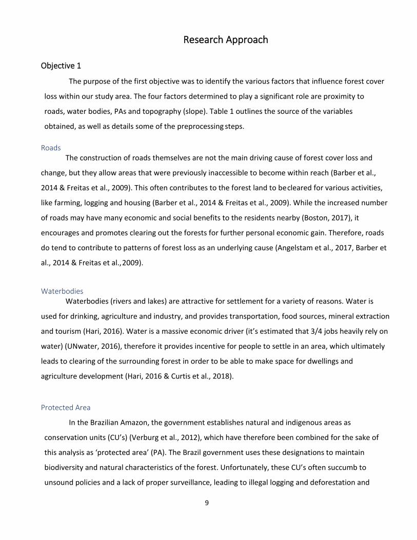
Research Approach Objective 1

The purpose of the first objective was to identify the various factors that influence forest cover

loss within our study area. The four factors determined to play a significant role are proximity to

roads, water bodies, PAs and topography (slope). Table 1 outlines the source of the variables

obtained, as well as details some of the preprocessing steps.

Roads The construction of roads themselves are not the main driving cause of forest cover loss and

change, but they allow areas that were previously inaccessible to become within reach (Barber et al.,

2014 & Freitas et al., 2009). This often contributes to the forest land to be cleared for various activities,

like farming, logging and housing (Barber et al., 2014 & Freitas et al., 2009). While the increased number

of roads may have many economic and social benefits to the residents nearby (Boston, 2017), it

encourages and promotes clearing out the forests for further personal economic gain. Therefore, roads

do tend to contribute to patterns of forest loss as an underlying cause (Angelstam et al., 2017, Barber et

al., 2014 & Freitas et al., 2009).

Waterbodies Waterbodies (rivers and lakes) are attractive for settlement for a variety of reasons. Water is

used for drinking, agriculture and industry, and provides transportation, food sources, mineral extraction

and tourism (Hari, 2016). Water is a massive economic driver (it’s estimated that 3/4 jobs heavily rely on

water) (UNwater, 2016), therefore it provides incentive for people to settle in an area, which ultimately

leads to clearing of the surrounding forest in order to be able to make space for dwellings and

agriculture development (Hari, 2016 & Curtis et al., 2018).

Protected Area

In the Brazilian Amazon, the government establishes natural and indigenous areas as

conservation units (CU’s) (Verburg et al., 2012), which have therefore been combined for the sake of

this analysis as ‘protected area’ (PA). The Brazil government uses these designations to maintain

biodiversity and natural characteristics of the forest. Unfortunately, these CU’s often succumb to

unsound policies and a lack of proper surveillance, leading to illegal logging and deforestation and

10

“paper parks” (Figueiredo, 2007 & Verburg et al., 2012). Over 60% of the borders of PAs are not

respected, primarily because they are lacking implementation of initiatives.

Topography/Slope Topography and variations in slope influence the ease of travel. Generally, areas with steeper

slope tend to experience less deforestation, whereas areas of lower elevation with gentler slopes are

often used for sugarcane plantations and ranches in the Amazon, contributing to clear-cutting (Freitas

et al., 2009 & Ranta et al., 1998). In addition, areas with steeper slopes often have lower-quality soil

and therefore experience less human use (Silva et al., 2007). Construction of the Transamazon

Highway and others in the Amazon tended to avoid areas with high slope (Arima et al., 205), therefore

slope and topography are likely contributing factors to rates of forest loss.

Table 1. Data sources and pre-processing requirements for data preparation.

Required Data Data Type Scale Year Source Pre-Processing Required

Forest Loss

(lossyear)

Raster 30mx30m 2000-2018 University of Maryland (Landsat & Landsat 8 OLI)

Download the lossyear raster for three areas (10N70W, 10N60W, 0N,70W) and mosaic them to encompass our study area and clip. Derive a binary raster for deforested areas and forested areas.

Important to note that this data is based on Landsat 8 imaging that identifies tree cover change over time and is subject to minor error.

Protected Area

(5 files in total – one for each area of protected land)

Vector (Shapefile, polygon)

N/A January 2020 (updated monthly)

Brazil’s Ministry of Justice and Public Security

Combine 5 shapefiles. Clip the protected areas to our necessary study area. Rasterization to 30mx30m. Generate a Euclidean distance raster.

DEM (slope)

(six files in total)

Raster (TIFF)

30mx30m 2000 USGS – Shuttle Radar Topography Mission

Create a mosaic of six DEM sections. Clip to study area. Derive slope.

Roads

(Roraima_roads)

Vector (shapefile, line)

N/A Most Recent OpenStreetMap; user community

Clip the roads to our necessary study area. Rasterization to 30mx30m. Generate a Euclidean distance raster.

11

Required Data Data Type Scale Year Source Pre-Processing Required

Water Features

(Roraima_rivers & Lago_jatapu)

Vector (shapefile, line and polygon)

N/A 2019 OpenStreetMap; user community

Clip the rivers to our necessary study area. Rasterization to 30mx30m. Generate a Euclidean distance raster.

Objective 2

The second objective was to create and design a model which considers the four variables that

were predicted to influence forest loss. This model was achieved using a similar technique to Bavaghar

(2015), as his methodology included the identification of variables that may be contributing to

deforestation, as well as a final logistic regression to generate a map of predicted deforested areas.

Preparation of data can be seen in Figures 4, 5 and 6. The final workflow to yield the end product can be

seen in Figure 7. A logistic regression was performed in RStudio that yielded the beta values to input

into the raster calculator to produce an output model which showed the probability that an area will

experience forest loss (Bavaghar, 2015 & Mohammadi et al., 2013) (Table 3). This output model was

then validated against the forest loss data from the University of Maryland, which can be seen in Figure

9.

12

Figure 4. Workflow to create the slope raster (Slope.tif). This raster acted as the extent for the analysis, therefore was created first. Six files were downloaded from the USGS’ Shuttle Radar Topography Mission, projected, mosaiced together, and then the slope was derived using the Slope Tool to yield the final slope.tif raster.

13

Figure 5. Workflow to obtain the Euclidean distance rasters for both waterbodies (EUC_rivers.tif) and roads (EUC_roads.tif).The process for both followed the same method. Vectors were converted to rasters, clipped to the slope.tif extent, reclassified into binary rasters and then a Euclidean distance raster was derived from each one.

14

Figure 6. Workflow to obtain the Euclidean distance raster for PAs, EUC_protected.tif. Five shapefiles (one for each PA) were converted to rasters, ad mosaiced to a new raster which was then clipped to the slope.tif extent. The combined PA raster was then reclassified to become binary, and a Euclidean distance raster was generated.

15

Figure 7. Workflow to create the forest loss raster. Beginning with four files from the Hansen et al. University of Maryland dataset, they were mosaiced and clipped to the slope.tif extent. The raster was split into forested and deforested, then each one was converted to a polygon. 100 random points were selected from both polygons, and the point files were merged. Multivalues were extracted and outputted as an excel table. Beta coefficients were then determined in R and the raster calculator was used to create the final raster, probability.tif.

Objective 3

The purpose of the third objective was to assess the accuracy of predicted forest loss using the

16

model developed in Objective 2. In order to validate our results, we followed a similar methodology to

Bavaghar (2015) as well as Hosmer & Lemeshow (2000). We validated the significance of each factor

and then determined the accuracy of the model when compared to the forest loss data. Factors were

validated based on the p coefficients. p coefficients, given by the output of the logistic regression, that

have a value lower than 0.05 are considered to be significant factors and any value higher will be

deemed insignificant (Hosmer & Lemeshow, 2000). The accuracy of the overall model was determined

through an Akaike Information Criterion (AIC), which is a statistical model that estimates out of sample

prediction error and therefore can determine the most appropriate model (Akaike, 1973). Four

different models were generated (Table 3) in order to determine the lowest AIC value, and the model

with the lowest value was therefore the model we used (Akaike, 1973). The probability values were

then acquired and compared to the University of Maryland Forest Loss data.

Objective 4 The purpose of the fourth objective was to evaluate the results of Objectives 2 and 3 for

strengths and weaknesses regarding selection of study site and chosen deforestation variables.

Although chosen for their perceived impact on deforestation, variables slope, rivers and PAs were

found to have insignificant impact. This remainder of objective is met in the following sections.

17

Research Findings

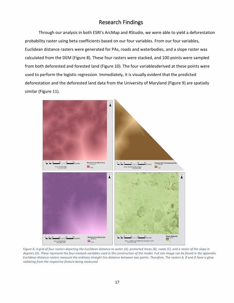
Through our analysis in both ESRI’s ArcMap and RStudio, we were able to yield a deforestation

probability raster using beta coefficients based on our four variables. From our four variables,

Euclidean distance rasters were generated for PAs, roads and waterbodies, and a slope raster was

calculated from the DEM (Figure 8). These four rasters were stacked, and 100 points were sampled

from both deforested and forested land (Figure 10). The four variablesderived at these points were

used to perform the logistic regression. Immediately, it is visually evident that the predicted

deforestation and the deforested land data from the University of Maryland (Figure 9) are spatially

similar (Figure 11).

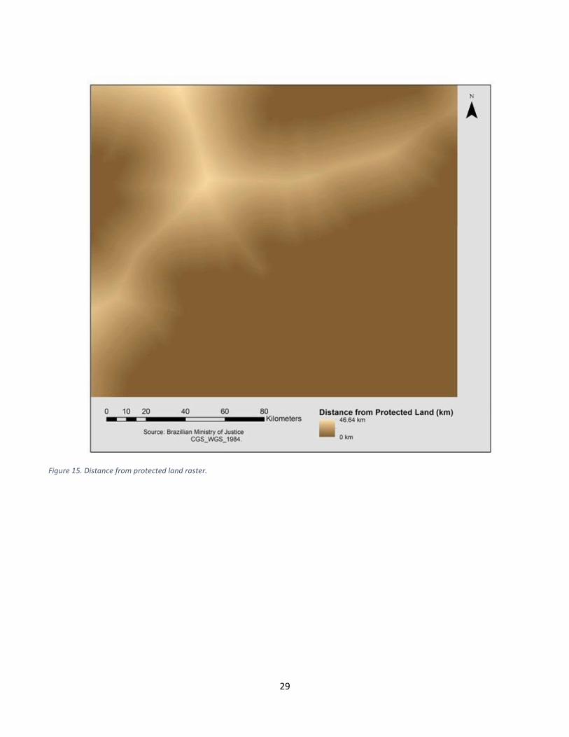
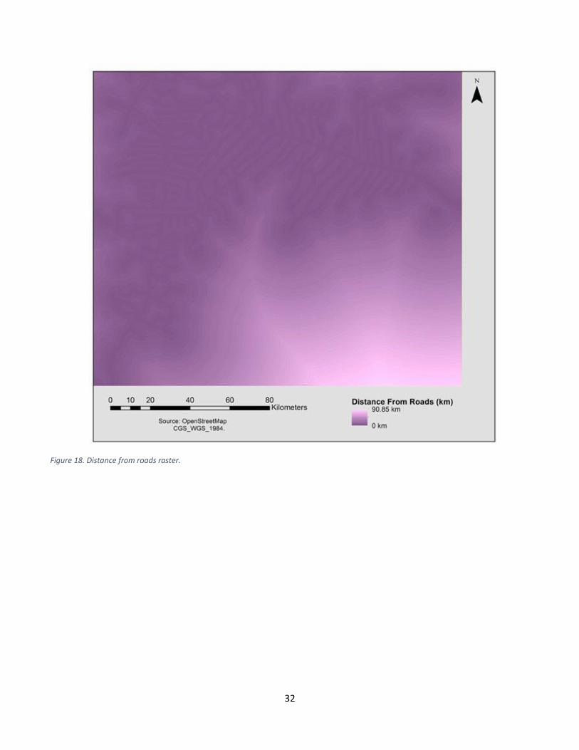
Figure 8. A grid of four rasters depicting the Euclidean distance to water (A), protected Areas (B), roads (C), and a raster of the slope in degrees (D). These represent the four analysis variables used in the construction of the model. Full size image can be found in the appendix. Euclidean distance rasters measure the ordinary straight line distance between two points. Therefore, The rasters A, B and D have a glow radiating from the respective feature being measured

18

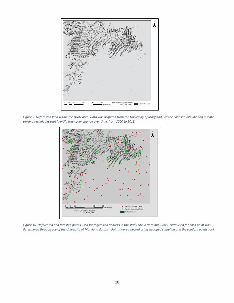
Figure 9. Deforested land within the study area. Data was acquired from the University of Maryland, via the Landsat Satellite and remote sensing techniques that identify tree cover change over time, from 2000 to 2018.

Figure 10. Deforested and forested points used for regression analysis in the study site in Roraima, Brazil. Data used for each point was determined through use of the University of Maryland dataset. Points were selected using stratified sampling and the random points tool.

19

Figure 11. Deforestation data from the University of Maryland in comparison to the predictive raster that was generated from the model. The predictive raster has a glow that radiates from the areas of current deforestation, immediately showing that the model was effective.

Based on the results from the logistic regression performed in R, we were able to determine

which of our predicted variables contributed to deforestation in our chosen study site. Roads

overwhelmingly had the highest correlation to deforestation, with a p value of 9.49e-05. Following this,

none of our other variables were determined to be statistically significant at a 95% confidence interval in

causing deforestation (PAs: p value of 0.527, slope: p value of 0.711 and water: p value of 0.861) (Table

2). The best model to predict deforestation in our study area does not include any variable besides

roads. This was determined based on the AIC (Akaike Information Criterion) (Table 3), which determines

which model is the best fit (Mohammed et al., 2015). Our findings show that a model using only roads

has the lowest AIC value and therefore was determined to be the best model (Figure 12).

20

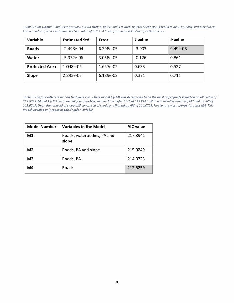
Table 2. Four variables and their p values: output from R. Roads had a p-value of 0.0000949, water had a p-value of 0.861, protected area had a p-value of 0.527 and slope had a p-value of 0.711. A lower p-value is indicative of better results.

Variable Estimated Std. Error Z value P value

Roads -2.498e-04 6.398e-05 -3.903 9.49e-05

Water -5.372e-06 3.058e-05 -0.176 0.861

Protected Area 1.048e-05 1.657e-05 0.633 0.527

Slope 2.293e-02 6.189e-02 0.371 0.711

Table 3. The four different models that were run, where model 4 (M4) was determined to be the most appropriate based on an AIC value of 212.5259. Model 1 (M1) contained all four variables, and had the highest AIC at 217.8941. With waterbodies removed, M2 had an AIC of 215.9249. Upon the removal of slope, M3 composed of roads and PA had an AIC of 214.0723. Finally, the most appropriate was M4. This model included only roads as the singular variable.

Model Number Variables in the Model AIC value

M1 Roads, waterbodies, PA and slope

217.8941

M2 Roads, PA and slope 215.9249

M3 Roads, PA 214.0723

M4 Roads 212.5259

21

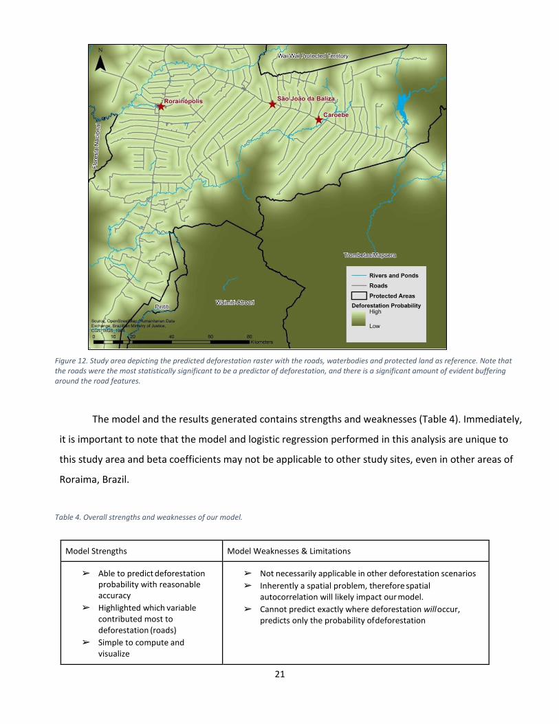
Figure 12. Study area depicting the predicted deforestation raster with the roads, waterbodies and protected land as reference. Note that the roads were the most statistically significant to be a predictor of deforestation, and there is a significant amount of evident buffering around the road features.

The model and the results generated contains strengths and weaknesses (Table 4). Immediately,

it is important to note that the model and logistic regression performed in this analysis are unique to

this study area and beta coefficients may not be applicable to other study sites, even in other areas of

Roraima, Brazil.

Table 4. Overall strengths and weaknesses of our model.

Model Strengths Model Weaknesses & Limitations

➢ Able to predict deforestation probability with reasonable accuracy

➢ Highlighted which variable contributed most to deforestation (roads)

➢ Simple to compute and visualize

➢ Not necessarily applicable in other deforestation scenarios ➢ Inherently a spatial problem, therefore spatial

autocorrelation will likely impact our model. ➢ Cannot predict exactly where deforestation will occur,

predicts only the probability of deforestation

22

Model Evaluation

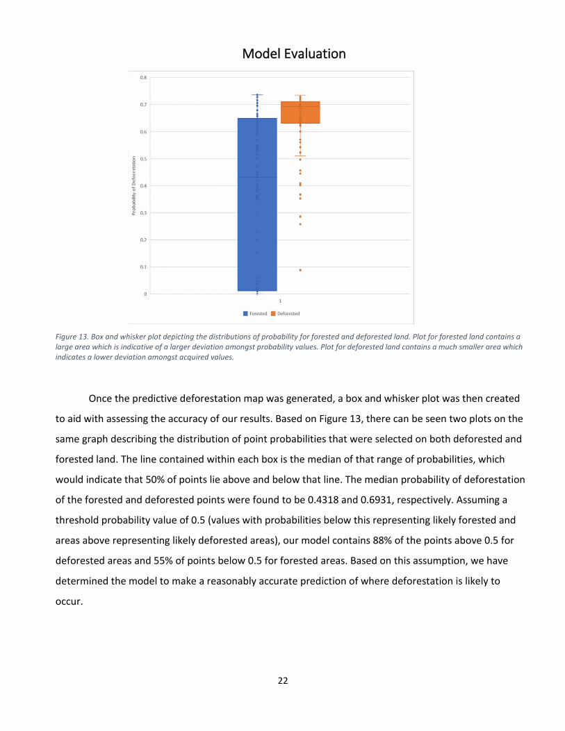
Figure 13. Box and whisker plot depicting the distributions of probability for forested and deforested land. Plot for forested land contains a large area which is indicative of a larger deviation amongst probability values. Plot for deforested land contains a much smaller area which indicates a lower deviation amongst acquired values.

Once the predictive deforestation map was generated, a box and whisker plot was then created

to aid with assessing the accuracy of our results. Based on Figure 13, there can be seen two plots on the

same graph describing the distribution of point probabilities that were selected on both deforested and

forested land. The line contained within each box is the median of that range of probabilities, which

would indicate that 50% of points lie above and below that line. The median probability of deforestation

of the forested and deforested points were found to be 0.4318 and 0.6931, respectively. Assuming a

threshold probability value of 0.5 (values with probabilities below this representing likely forested and

areas above representing likely deforested areas), our model contains 88% of the points above 0.5 for

deforested areas and 55% of points below 0.5 for forested areas. Based on this assumption, we have

determined the model to make a reasonably accurate prediction of where deforestation is likely to

occur.

23

Discussion

Roads were determined to be the most impactful on deforestation. Distance to water,

protected areas (PAs) and relative slope were determined to have an insignificant effect on

deforestation in our study site with given analysis methods. These results contradict the results from

Bavaghar (2015), which claimed that slope was a significant factor. One explanation for this could be

that the land is relatively flat in our study area compared to that of Bavaghar (2015) which took place

in Iran. This could indicate that relative steepness of the slopes plays a much larger impact. PAs

having an insignificant impact on deforestation could indicate that these areas are not being

protected. We would assume that the PAs would have an inverse relationship with deforestation due

to the sites being preserved. This could be indicative of our selected PA’s being part of the “paper

parks” phenomenon where an area is selected for protection, but is not protected due to lack of

resources (Figueiredo, 2007 & Verburg et al., 2012). Water also having insignificant impact on

deforestation in this area is interesting, as it could mean that the study area’s economy does not

heavily rely on water specifically from rivers and ponds for agriculture development. The study area

falls within the Coastal Plain groundwater province in Brazil, where large amounts of groundwater can

be easily obtained from artesian wells (Schneider, 1963). This could imply that the study area already

has an effective irrigation and water system, meaning being in close proximity to water is not a

concern. However, it is important to note that the direct presence of water was not deemed a

significant driving factor of deforestation.

Conclusions

The purpose of this research was to create a predictive deforestation model using a logistic

regression-based analysis which would determine which factor(s) is most influential to deforestation.

Roads were determined to be the most significant factor contributing to deforestation in our study area

based on our model and our outputs. This points to roads as the lead driver in deforestation, however,

our model does not explain why the deforestation was heavily reliant on the presence of roads.

Waterbodies, PAs and slope were not found to significantly contribute to the probability of

deforestation.

The overall goal of this project was not to compute a model applicable worldwide, but to

be predictive in nature for the selected study site. In continuing this work, selection of study site

24

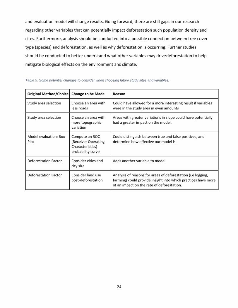
and evaluation model will change results. Going forward, there are still gaps in our research

regarding other variables that can potentially impact deforestation such population density and

cites. Furthermore, analysis should be conducted into a possible connection between tree cover

type (species) and deforestation, as well as why deforestation is occurring. Further studies

should be conducted to better understand what other variables may drive deforestation to help

mitigate biological effects on the environment and climate.

Table 5. Some potential changes to consider when choosing future study sites and variables.

Original Method/Choice Change to be Made Reason

Study area selection Choose an area with less roads

Could have allowed for a more interesting result if variables were in the study area in even amounts

Study area selection Choose an area with more topographic variation

Areas with greater variations in slope could have potentially had a greater impact on the model.

Model evaluation: Box Plot

Compute an ROC (Receiver Operating Characteristics) probability curve

Could distinguish between true and false positives, and determine how effective our model is.

Deforestation Factor Consider cities and city size

Adds another variable to model.

Deforestation Factor Consider land use post-deforestation

Analysis of reasons for areas of deforestation (i.e logging, farming) could provide insight into which practices have more of an impact on the rate of deforestation.

25

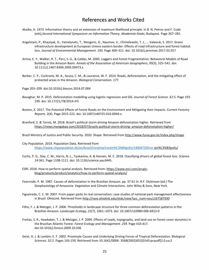
References and Works Cited

Akaike, H. 1973. Information theory and an extension of maximum likelihood principle. In B. N. Petrov and F. Csaki (eds),Second International Symposium on Information Theory, Akademiai Kiado, Budapest. Page 267–281.

Angelstam, P., Khaulyak, O., Yamelynets, T., Mozgeris, G., Naumov, V., Chmielewski, T. J., … Valasiuk, S. 2017. Green infrastructure development at European Unions eastern border: Effects of road infrastructure and forest habitat loss. Journal of Environmental Management. 193. Page 300–311. doi: 10.1016/j.jenvman.2017.02.017

Arima, E. Y., Walker, R. T., Perz, S. G., & Caldas, M. 2005. Loggers and Forest Fragmentation: Behavioral Models of Road Building in the Amazon Basin. Annals of the Association of American Geographers, 95(3), 525–541. doi: 10.1111/j.1467-8306.2005.00473.x

Barber, C. P., Cochrane, M. A., Souza, C. M., & Laurance, W. F. 2014. Roads, deforestation, and the mitigating effect of protected areas in the Amazon. Biological Conservation. 177.

Page 203–209. doi:10.1016/j.biocon.2014.07.004

Bavaghar, M. P. 2015. Deforestation modelling using logistic regression and GIS. Journal of Forest Science. 61:5. Page 193-199. doi: 10.17221/78/2014-JFS

Boston, K. 2017. The Potential Effects of Forest Roads on the Environment and Mitigating their Impacts. Current Forestry Reports. 2(4). Page 2015-222. doi: 10.1007/s40725-016-0044-x

Branford, S. & Torres, M. 2018. Brazil’s political storm driving Amazon deforestation higher. Retrieved from https://news.mongabay.com/2018/07/brazils-political-storm-driving- amazon-deforestation-higher/

Brazil Ministry of Justice and Public Security. 2020. Shape. Retrieved from http://www.funai.gov.br/index.php/shape

City Population. 2019. Population Data. Retrieved from https://www.citypopulation.de/en/brazil/roraima/rorain%C3%B3polis/140047205ror ain%C3%B3polis/

Curtis, P. G., Slay, C. M., Harris, N. L., Tyukavina, A. & Hansen, M. C. 2018. Classifying drivers of global forest loss. Science. 14:361. Page 1108-1111. doi: 10.1126/science.aau3445.

ESRI. 2018. How to perform spatial analysis. Retrieved from: https://www.esri.com/arcgis- blog/products/product/analytics/how-to-perform-spatial-analysis/

Fearnside, P. M. 1987. Causes of deforestation in the Brazilian Amazon. pp. 37-61 In: R.F. Dickinson (ed.) The Geophysiology of Amazonia: Vegetation and Climate Interactions. John Wiley & Sons, New York.

Figueiredo, C. C. M. 2007. From paper parks to real conservation: case studies of national park management effectiveness in Brazil. OhioLink. Retrieved from http://rave.ohiolink.edu/etdc/view?acc_num=osu1167587930

Filho, F. J. & Metzger, J. P. 2006. Thresholds in landscape structure for three common deforestation patterns in the Brazilian Amazon. Landscape Ecology, 21(7), 1061–1073. doi: 10.1007/s10980-006-6913-0

Freitas, S. R., Hawbaker, T. J. & Metzger, J. P. 2009. Effects of roads, topography, and land use on forest cover dynamics in the Brazilian Atlantic Forest. Forest Ecology and Management. 259. Page 410-417. doi:10.1016/j.foreco.2009.10.036

Geist, H. J. & Lambin, E. F. 2002. Proximate Causes and Underlying Driving Forces of Tropical Deforestation. Biological Sciences. 52:2. Pages 143-150. Retrieved from 10.1641/0006- 3568(2002)052[0143:pcaudf]2.0.co;2

26

Hansen, M. C., Potapov, P. V., Moore, R., Hancher, M., Turubanova, S. A., Tyukavina, A., … Townshend, J. R. G. 2019. High-Resolution Global Maps of 21st-Century Forest Cover Change. Science, 342(6160), 850–853. doi: 10.1126/science.1244693

Hari, S. 2016. Communities along Rivers: Importance of Community Networking to Preserve Local Rivers. Retrieved from http://www.gdrc.org/oceans/river-mgmt.html

Hashimoto, H., Melton, F., Ichii, K., Milesi, C., Wang, W., & Nemani, R. R. 2010. Evaluating the impacts of climate and elevated carbon dioxide on tropical rainforests of the western Amazon basin using ecosystem models and satellite data. Global Change Biology. 16(1). Page 255–271. doi: http://10.1111/j.1365-2486.2009.01921.x

Hosmer, D. W. & Lemeshow, S. 2000. Applied Logistic Regression: 2nd Edition. John Wiley & Sons, Inc.

Humanitarian Data Exchange. 2020. Brazil administrative boundaries. Retrieved from: https://data.humdata.org/dataset/brazil-administrative-level-0-boHundaries

IPCC. 2019. Climate Change and Land: an IPCC special report on climate change, desertification, land degradation, sustainable land management, food security, and greenhouse gas fluxes in terrestrial ecosystems [P.R. Shukla, J. Skea, E. Calvo Buendia, V. Masson- Delmotte, H.-O. Pörtner, D. C. Roberts, P. Zhai, R. Slade, S. Connors, R. van Diemen, M. Ferrat, E. Haughey, S. Luz, S. Neogi, M. Pathak, J. Petzold, J. Portugal Pereira, P. Vyas, E. Huntley, K. Kissick, M. Belkacemi, J. Malley, (eds.)]. In press. Retrieved from: https://www.ipcc.ch/srccl/

Krummer, D. & Sham, C. H. 1994. The causes of tropical deforestation: a quantitative analysis and case study from the Philippines. London, England: UCL Press.

Lewinsohn, T. M. & Prado, T. I. 2005. How Many Species Are There in Brazil? Conservation Biology. 19(3). Page 619-624. doi: https://doi.org/10.1111/j.1523-1739.2005.00680.x

Marchand, S. 2012. The relationship between technical efficiency in agriculture and deforestation in the Brazilian Amazon. Ecological Economics. 77. Page 166-175. doi: 10.1016/j.ecolecon.2012.02.025

Mohammadi, F., Bavaghar, M. P., & Shabanian, N. 2013. Forest Fire Risk Zone Modeling Using Logistic Regression and GIS: An Iranian Case Study. Small-Scale Forestry. 13(1), Page 117–125. doi: 10.1007/s11842-013-9244-4

Mohammed, E. A., Naugler, C., & Far, B. H. 2015. Emerging Business Intelligence Framework for a Clinical Laboratory Through Big Data Analytics. Emerging Trends in Computational Biology, Bioinformatics, and Systems Biology. Pages 577–602. doi: 10.1016/b978-0-12- 802508-6.00032-6

Mongabay. 2020. Amazon Destruction. Retrieved from https://rainforests.mongabay.com/amazon/amazon_destruction.html

OSM Foundation. 2020. FAQ’s. Retrieved from https://blog.openstreetmap.org/faq/

Ranta, P., Blom, T., Niemela, J., Joensuu, E. & Siitonen, M. 1998. The Fragmented rain forest of Brazil: size, shape, and distribution of forest fragments. Biodiversity and Conservation. 7. Page 385-403. Retrieved from https://link.springer.com/content/pdf/10.1023%2FA%3A1008885813543.pdf

Rosa, I. M., Purves, D., Souza, C. & Ewers, R. M. 2013. Predictive Modelling of Contagious Deforestation in the Brazilian Amazon. PloS One. 8:10. doi: 10.1371/journal.pone.0077231

Schneider, R. 1963. Ground-water provinces of Brazil. US Department of the Interior. Retrieved from https://pubs.usgs.gov/wsp/1663a/report.pdf

Silva, W. G., Metzger, J. P., Simoes, S. & Simonetti, C. 2007. Relief influence on the spatial distribution of the Atlantic Forest cover on the Ibiúna Plateau, SP. Brazilian Journal of Biology. 67:3. Retrieved from

27

http://dx.doi.org/10.1590/S1519-69842007000300004

Thapa, R. B. and Murayama, Y. 2009. Accuracy of Land Use and Land Cover Mapping Methods.

Retrieved from https://link-springer- com.subzero.lib.uoguelph.ca/content/pdf/10.1007%2F978-94-007-0671-2.pdf

United Nations. 2016. The United Nations World Water Development Report 2016: Water and Jobs. Retrieved from https://unesdoc.unesco.org/ark:/48223/pf0000243938

University of Maryland. 2020. Global Forest Change 2000–2018

Data Download. Retrieved from: https://earthenginepartners.appspot.com/science- 2013-global-forest/download_v1.6.html

Verburg, R., Filho, S. R., Lindoso, D., Debortoli, N., Litre, G. & Bursztyn, M. 2012. The impact of commodity price and conservation policy scenarios on deforestation and agricultural land use in a frontier area within the Amazon. Land Use Policy. 37. Page 14-26.

Retrieved from http://dx.doi.org/10.1016/j.landusepol.2012.10.003"http://dx.doi.org/10.1016/j.landus epol.2012.10.003

Weisse, M. J., & Naughton-Treves, L. C. (2016). Conservation Beyond Park Boundaries: The Impact of Buffer Zones on Deforestation and Mining Concessions in the Peruvian Amazon. Environmental Management, 297-311. Retrieved from: https://link.springer.com/article/10.1007/s00267-016-0709-z

Wells, M. P. & Brandon, K. E. 1993. The Principles and Practice of Buffer Zones and Local Participation in Biodiversity Conservation. Ambio. Page 157-162. Retrieved from https://www-jstor-org.subzero.lib.uoguelph.ca/stable/4314061

World Wildlife Federation. 2020. Amazon. Retrieved from: https://www.worldwildlife.org/places/amazon

28

Appendices

Figure 14. Full flow chart depicting the entire workflow.

29

Figure 15. Distance from protected land raster.

30

Figure 16. Slope raster.

31

Figure 17. Distance from water raster.

32

Figure 18. Distance from roads raster.