Analyzing The Dynamic Nature Of The Economic Factors

Mathematical Theory and Modeling www.iiste.org

ISSN 2224-5804 (Paper) ISSN 2225-0522 (Online)

Vol.5, No.4, 2015

106

Analyzing The Dynamic Nature Of The Economic Factors: An

Application of VAR Model and IRF

Adam H. Yagoob(1*)

; Qian Zhengming (2)

1. School of Economics, Department of Statistics & Planning; Xiamen University,

Room No. 607, Cia Qingjie Build. 361005 Xiamen, Fujian, China.

*E-mail: [email protected]; [email protected]

2. School of Economics, Department of Statistics & Planning Xiamen University,

361005 Xiamen, Fujian P.R. China

Abstract

This paper uses vector autoregressive model and impulse response function to assess the external debt

sustainability of Sudan. It aims to analyse the dynamic and long term effects among economic indicators and

capture response of economic variable to a shock in another variable. Also, to determine the factors that impact a

nation’s struggle to maintain debt at sustainable levels. A precise list of indicators of indebtedness was inserted

in the model. Results showed that indicators of indebtedness are predictable using measures of repayment

capacity. In contrast, the domestic repayment capacities are not possible to be predicted, using indicators of

indebtedness; and significantly affects the indebtedness of Sudan, hence, Policies to enhance the use of domestic

resources to repay debts are recommended. As cost based indicators of indebtedness, significantly affect the

exports growth, they should be maintained at a sustainable level.

Keywords: VAR, IRF, External debt, Repayment capacity,Economic Growth, Sudan

1. Introduction

An economic entity, say a nation, is likely to have income that exceeds the expenditure and at the same time,

another nation’s expenses might increase the level of income. In such a scenario, borrowing and lending

encourage the economic growth in both nations. Debt creation makes them able to realize the output preferences

and intertemporal consumption. One of the assumptions in debt creation is the fulfillment of the debt

requirements by the debtor. Problems arise when the income of the debtor country is insufficient or assets that

are useful in case of insufficient income are inadequate. In the existence of this problem, or even if it is not

raised but only anticipated, both the creditor and debtor countries may not realize the benefits of international

financial flow. Hence, nations need to involve in the risk-management procedures and to maintain the external

debt at sustainable levels.

The difficult economic condition of Sudan was exacerbated by the country’s export base and revenue contracting

sharply. Hence, the country’s debt servicing capacity is seriously reduced due to the severely affected macro-

economic outlook; followed by permanent shock. A so-called zero point is achieved in an agreement between

Sudan and South Sudan before the secession of South Sudan, which stated retaining all the external liabilities of

Sudan after the South Sudan secession provided that; within two years from the secession, the delivery of debt

relief is committed by the international community and debt relief of Sudan will be assisted by South Sudan. A

pending formula will then determine the apportionment of Sudan’s external debt if the commitments are not

made. This paper is an application of VAR model and IRF to perform external debt sustainability analysis of

Sudan. Hence, it determines the factors impacting external debt sustainability of Sudan.

brought to you by COREView metadata, citation and similar papers at core.ac.uk

provided by International Institute for Science, Technology and Education (IISTE): E-Journals

https://core.ac.uk/display/234680056?utm_source=pdf&utm_medium=banner&utm_campaign=pdf-decoration-v1

http://www.iiste.org/

mailto:[email protected]

mailto:[email protected]



Vol.5, No.4, 2015

107

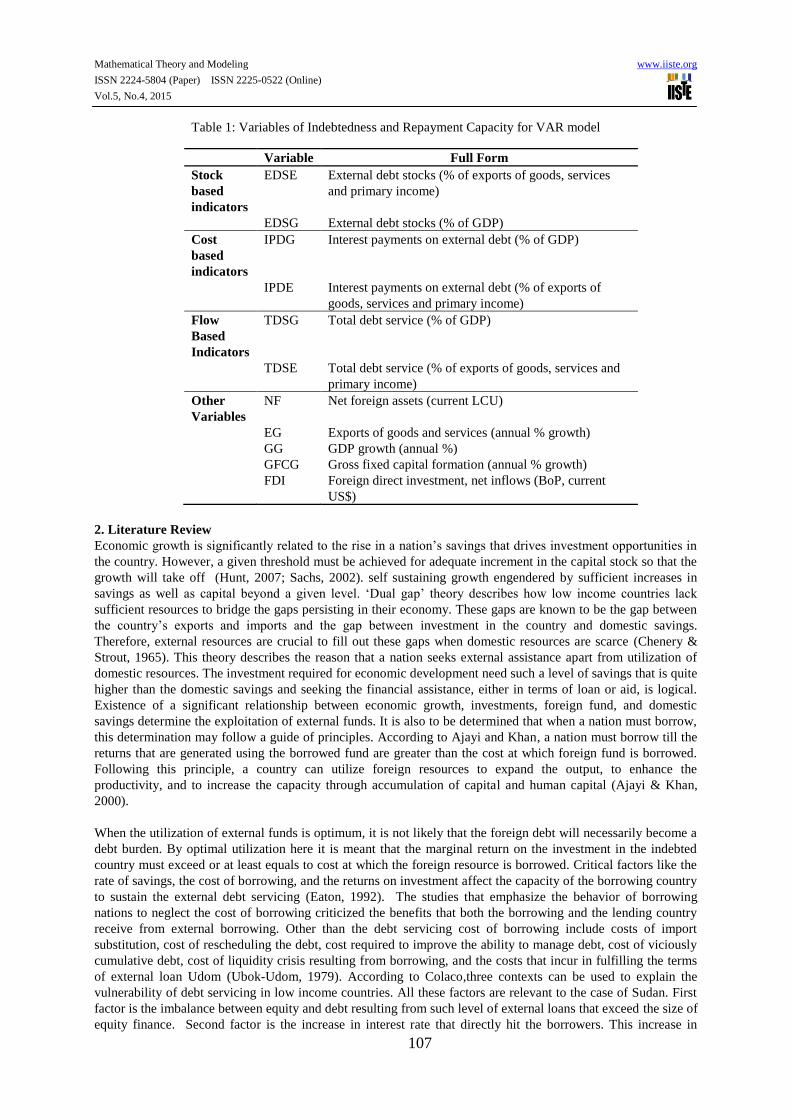
Table 1: Variables of Indebtedness and Repayment Capacity for VAR model

Variable Full Form

Stock

based

indicators

EDSE External debt stocks (% of exports of goods, services

and primary income)

EDSG External debt stocks (% of GDP)

Cost

based

indicators

IPDG Interest payments on external debt (% of GDP)

IPDE Interest payments on external debt (% of exports of

goods, services and primary income)

Flow

Based

Indicators

TDSG Total debt service (% of GDP)

TDSE Total debt service (% of exports of goods, services and

primary income)

Other

Variables

NF Net foreign assets (current LCU)

EG Exports of goods and services (annual % growth)

GG GDP growth (annual %)

GFCG Gross fixed capital formation (annual % growth)

FDI Foreign direct investment, net inflows (BoP, current

US$)

2. Literature Review

Economic growth is significantly related to the rise in a nation’s savings that drives investment opportunities in

the country. However, a given threshold must be achieved for adequate increment in the capital stock so that the

growth will take off (Hunt, 2007; Sachs, 2002). self sustaining growth engendered by sufficient increases in

savings as well as capital beyond a given level. ‘Dual gap’ theory describes how low income countries lack

sufficient resources to bridge the gaps persisting in their economy. These gaps are known to be the gap between

the country’s exports and imports and the gap between investment in the country and domestic savings.

Therefore, external resources are crucial to fill out these gaps when domestic resources are scarce (Chenery &

Strout, 1965). This theory describes the reason that a nation seeks external assistance apart from utilization of

domestic resources. The investment required for economic development need such a level of savings that is quite

higher than the domestic savings and seeking the financial assistance, either in terms of loan or aid, is logical.

Existence of a significant relationship between economic growth, investments, foreign fund, and domestic

savings determine the exploitation of external funds. It is also to be determined that when a nation must borrow,

this determination may follow a guide of principles. According to Ajayi and Khan, a nation must borrow till the

returns that are generated using the borrowed fund are greater than the cost at which foreign fund is borrowed.

Following this principle, a country can utilize foreign resources to expand the output, to enhance the

productivity, and to increase the capacity through accumulation of capital and human capital (Ajayi & Khan,

2000).

When the utilization of external funds is optimum, it is not likely that the foreign debt will necessarily become a

debt burden. By optimal utilization here it is meant that the marginal return on the investment in the indebted

country must exceed or at least equals to cost at which the foreign resource is borrowed. Critical factors like the

rate of savings, the cost of borrowing, and the returns on investment affect the capacity of the borrowing country

to sustain the external debt servicing (Eaton, 1992). The studies that emphasize the behavior of borrowing

nations to neglect the cost of borrowing criticized the benefits that both the borrowing and the lending country

receive from external borrowing. Other than the debt servicing cost of borrowing include costs of import

substitution, cost of rescheduling the debt, cost required to improve the ability to manage debt, cost of viciously

cumulative debt, cost of liquidity crisis resulting from borrowing, and the costs that incur in fulfilling the terms

of external loan Udom (Ubok-Udom, 1979). According to Colaco,three contexts can be used to explain the

vulnerability of debt servicing in low income countries. All these factors are relevant to the case of Sudan. First

factor is the imbalance between equity and debt resulting from such level of external loans that exceed the size of

equity finance. Second factor is the increase in interest rate that directly hit the borrowers. This increase in




Vol.5, No.4, 2015

108

interest rate results from the dramatic rise in the proportion of debt at floating interest rate. Third factor is the

drastic shortfalls in maturities resulting from the decline in share of financial flows (Colaco, 1985). The

increasing complexity in the financial environment essentially requires adequate debt management whose critical

components are statistical analysis, accounting, regulatory environment, and policy coordination . Structural

reforms and fiscal adjustment adopted in the debtor nation help in making the measures effective needed to

support the process of development in the debtor nation. Decision making processes, improvement or sometimes

creation of debt management structure, and anticorruption and transparency policies are included in the features

of debt management(Mehran, 1985). Still the issue remains that whether sustainability of debt is assured by

acquisition and management of external fund.

Macroeconomic instability and tax disincentive are the debt overhang effects of accumulated debt stock that

reduces economic performance. Macroeconomic instability is related to the anticipated inflation, possible

monetary expansion, depreciation in the exchange rate, exceptional financing resulting in uncertainly, and rise in

fiscal deficit. By debt disincentive, it is meant that the anticipation of large taxes in future income to cover the

increasing debt burden in present discourage investments (Claessens, World, et al., 1996). Private investment is

also found to be negatively impacted by external debt as results in the study by Iyoha,affirmed the debt overhang

effect and crowding our effect of debt servicing. The author presented empirical justification that how these two

damaging effects of debt servicing leads to low level of private investment in the borrowing country (Iyoha,

1997). Efficient utilization of external financing is found to be the key factor that drives the rise in economic

development process. It happens that a country experiences growth in economic condition as long as the external

resources are efficiently utilized but as soon as the acquisition of foreign loan become inefficient, process of

economic growth slows down. Development of capital markets, restructuring the programs of sustained export

promotion, and privatization are preventive measures for the severe impact of external debt on public and private

investments whose major factors are global interest rates, balance of payments, and fiscal expenditure (Edo,

2002). African Fourm Network on Debt and Development (2003), recognizing the impacts of increasing external

debt states that integration within and across the African countries with regional groupings is de-accelerated by

the reliance of Africa on northern countries for hard currencies and heavy indebtedness. For a given level of

indebtedness in the future, the current level of investment is curbed by the high debt servicing in the present

which is another aspect of liquidity crisis resulting from external debt(Claessens, Detragiache, Kanbur, &

Wickbam, 1996). Apart the liquidity crisis, moral hazard effect is also identified as a damaging consequence of

external debt. According to Arnone et al. (2005), Moral hazard is evident in countries with poor macroeconomic

policies and high levels of external debt(Arnone, Bandiera, & Presbitero, 2005).

3. Methodology

Time series data is collected for this paper, the data includes the indicators of external debt and capacity to repay

of Sudan from 1970 to 2012. Time series include all the variables listed in Table 1.

3.1 Vector Autoregressive Model (VAR)

As the study employees VAR, each of the variables is endogenous and thus multiple regression equations are

estimated. There are 11 equations and 11 variables in the model. The dependent variable in each equation is

explained by its own value in previous two years and the values of the remaining 10 variables in the previous

two years. A VAR model is a supplementary of a system of equations whose purpose is to capture the dynamic

effects, thus; the 11 variables incorporated in the VAR model are together regarded as a vector Vt. Each of the

variables in Vt is assumed to be demeaned before estimating the model. Hence, none of the 11 equations have

intercept (constant) term. The so-called structural form of the VAR model thus becomes:

α Vt = β1 Vt-1 + β2 Vt-2 + … + βk Vt-k + εt … (1)

Eεε’ = ∑ε = [𝜌𝜀1

2 ⋯ 0⋮ ⋱ ⋮0 ⋯ 𝜌𝜀𝑛

2] … (2)

A VAR of lag length p(VAR(p)) can be written as:

vt = α-1

β1 vt-1 + α-1

β2 vt-2 + … + α-1

βk vt-k + α-1

εt … (3)

Where, E (εt) = 0, E (εt ε’t) = ∑ε for t = τ ; and 0 otherwise. The reduced form of equation 3 includes the past

values of the dependent variable and the past values of all other variables. There are three forms of a VAR




Vol.5, No.4, 2015

109

model, namely structure, recursive, and reduced. Identification of a VAR model is essential in each of the three

forms. Recovery of the estimation of α, β, and ∑ε is regarded here as identification of a VAR model. Here, the

model specifications are given taking only one lagged value in the VAR model for the sake of generality as

inclusion of more lag values is dealt in the same way. Each variable is presented as a linear combination of the

lagged values of the variable and the lagged values of the other variables in the reduced VAR model. Ordinary

Least Square (OLS) method is used to estimate each of the equation presenting linear relationship. After taking

the past values in account, the shock movements in the variables are regarded as error terms. Correlation in

among the error terms exists if a correlation exists among the variables. The α’s and the ∑ε are not easy to

estimate despite of the easy estimations of α-1

β1, …, α-1

βk and α-1

∑ε α-1

’ in the structural form of a VAR. In a

recursive VAR model, error term in each regression equation is assumed to be uncorrelated with the error terms

in the preceding equations. This assumption is made on the basis that the contemporaneous values of other

variables are included in some of the equations as regressors in estimating the VAR equations. The model in this

paper includes 11 variables and 11 equations but here for simplicity a 2-variables 2-equations VAR model is

presented to describe the specification. Once the procedure is clearly specified, model with the 11 variables will

be given. Following is a simple bivariate model with Debt Stock as Y and repayment capacity as X.

Yt = –αYXXt + βYXXt-1 + βYYYT-1 + εYT … (4)

Xt = –αXYXt + βXXXt-1 + βXYYT-1 + εXT … (5)

Where, structural parameters are αYX, αXY, βYX, βXX, βYY, and βXY and the uncorrelated structural shocks are εYT

and εXT with a standard deviation ρX and ρY. OLS cannot be used to estimate equation 4 and equation 5 because

the classical assumption of no correlation between the error term and the regressors is violated. If equation 5 is

estimated using OLS, the correlation between Y and the error terms exists, since:

cov(Yt, Xt) = cov(–αYXXt + βYXXt-1 + βYYYt-1 + Yt,Xt) =

= cov(–αYX (βXXXt-1 + βXYYt-1 – αXYYt + Xt) + βYXXt-1 + βYYYt-1 + Yt,Xt) =

= αYXαXYcov(Yt, Xt) – αYX 𝜌𝜀𝑋2

cov(Yt, Xt) = −αYX

1− αYXαXY 𝜌𝜀𝑋

2 … (6)

Unless αYX = 0 is assumed, the estimation of the parameters in equation 5 using OLS is inconsistent. This implies

that there is no effect of the repayment capacity on the debt stock. If a condition αYX = 0 is imposed, then the

OLS estimates of the parameters of equation 5 will not be inconsistent. A repayment capacity shock Xt = 1 will

not affect Yt while its effect on Xt will be equal to 1. Effect of a debt stock shock Yt on Yt will be 0. Effect of

debt stock shock Yt on Yt will be 1 if –αXY has an effect on Xt. As the OLS method is employed for estimation of

the equations one by one, this approach of estimation is used in recursive VAR. One exception made in this

paper is that Yt is included among the regressors in equation 5 while Xt is excluded from the regressors in

equation 4. Another more precise explanation of the use of OLS in estimating VAR model is the matrix form of

the equations. Let the following VAR model be a structural model that cannot be estimated using OLS:

[1 𝛼𝑌𝑋

𝛼𝑋𝑌 1] [

𝑌𝑡

𝑋𝑡] = [

𝛽𝑌𝑌 𝛽𝑌𝑋

𝛽𝑋𝑌 𝛽𝑋𝑋] [

𝑌𝑡−1

𝑋𝑡−1]+[

𝑌𝑡

𝑋𝑡] … (7)

The reduced form of equation 7 is:

[𝑌𝑡

𝑋𝑡] = [

1 𝛼𝑌𝑋

𝛼𝑋𝑌 1]

−1

[𝛽𝑌𝑌 𝛽𝑌𝑋

𝛽𝑋𝑌 𝛽𝑋𝑋] [

𝑌𝑡−1

𝑋𝑡−1]+ [

1 𝛼𝑌𝑋

𝛼𝑋𝑌 1]

−1

[𝑌𝑡

𝑋𝑡] … (8)

OLS can be used to estimate the reduced form of equation 7 in equation 8. This is because the structural

parameters cannot be identified from the residuals of the two equations; hence, there is a correlation among the

error terms of the equation 7 and equation 8 across the equations. Link between the structural parameters and the

residuals of the reduced form equation 7 and 8 are given by:

r1t = 1

1− αYXαXY (Yt – αYXXt) … (9)




Vol.5, No.4, 2015

110

r2t = 1

1− αYXαXY (Xt – αXYYt) … (10)

If αYX = 0, then:

r1t = Yt … (11)

r2t = Xt – αXYYt … (12)

Following the above information, two major steps in the procedure are identified. The first step is the estimation

of the reduced form equation through regressing Y on its lagged values and the lagged values of X recovering

the structural shock Yt. The second step follows from the realization that if the assumption αYX = 0 is made, the

estimates of equation 5 using OLS are consistent. Hence, Xt = –αXYYt + βXXXt-1 + βXYYt-1 + Xt is estimated and

the residuals are calculated to recover Xt. Structural parameters are easy to estimate in this way for the dynamic

system developed in equation 4 and equation 5. There might be confusion that using reduced form to estimate

equation 4 and excluding contemporaneous regressors to estimate equation 5, and so on for the actual 11

equations and 11 variables is the algorithm of the VAR jargon. The following two steps are involved instead:

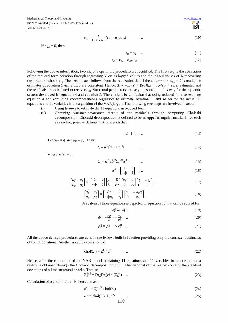
(i) Using Eviews to estimate the 11 equations in reduced form.

(ii) Obtaining variance-covariance matrix of the residuals through computing Choleski

decomposition. Choleski decomposition is defined to be an upper triangular matrix for each

symmetric, positive definite matrix Z such that:

Z =’ … (13)

Let αXY = ϕ and ρ12 = ρz. Then:

Zt = α-1

βzt-1 + α-1t … (14)

where α-1t = rt

r = α-1

1/21/2α

-1’ … (15)

α-1

= [1 0

– ϕ 1] … (16)

[𝜌1

2 𝜌𝑍

𝜌𝑍 𝜌22] = [

1 0

– ϕ 1] [

𝜌𝑌 00 𝜌𝑋

] [𝜌𝑌 00 𝜌𝑋

] [1 – ϕ 0 1

] … (17)

[𝜌1

2 𝜌𝑍

𝜌𝑍 𝜌22] = [

𝜌𝑌 0

– ϕ𝜌𝑌 𝜌𝑋

] [𝜌𝑌 – 𝜌𝑌ϕ0 𝜌𝑋

] … (18)

A system of three equations is depicted in equation 18 that can be solved for:

𝜌𝑌2 = 𝜌1

2 … (19)

𝜙 =–𝜌𝑋

𝜌𝑌2 = –

𝜌𝑋

𝜌12 … (20)

𝜌𝑋2 = 𝜌2

2 − ϕ2𝜌12 … (21)

All the above defined procedures are done in the Eviews built in function providing only the consistent estimates

of the 11 equations. Another notable expression is:

chol(r) = 1/2α

-1’ … (22)

Hence, after the estimation of the VAR model containing 11 equations and 11 variables in reduced form, a

matrix is obtained through the Choleski decomposition of r. The diagonal of the matrix contains the standard

deviations of all the structural shocks. That is:

1/2 = Dg(Dg(chol(r))) … (23)

Calculation of α and/or α-1

.α-1

is then done as:

α-1

’ = −1/2 chol(r) … (24)

α-1

= chol(r)’ −1/2 … (25)




Vol.5, No.4, 2015

111

The contemporaneous relationships among the variables as estimated in the structural VAR model are sorted out

using economic theory. For example, if economic theory suggests that αYX = –0.5, then only the

contemporaneous effect of shocks do not need to be involved in the assumptions.

3.2 Impulse Response Function (IRF)

Impulse response functions (IRF) are often obtained in a VAR model. IRF captures the effect of one-unit

increase or an increase equal to one standard deviation in the current values of the VAR errors on the current or

future values of each of the variables included in the VAR model. Assumption made in obtaining IRF include

that in subsequent periods, the effecting error returns to zero and all the other errors are equal to zero. IRF is

typically obtained in structural and recursive VAR models as the process of estimating effect one error shock,

keeping other error terms constant is appropriate only if the error terms are correlated across the equations. If α

and are known, the procedure of obtaining IRF begins from:

Zt = α-1

βzt-1 + α-1t… (26)

Where, α-1t = rt. Once, α

-1 is known, the IRF’s can be calculated to a unit shock of assuming that for a while,

the system is in steady state. Consider that a two-variable VAR is obtained and the dynamics to a shock to the

first variable are to be obtained. If a shock hits at time, t = 0, then:

0 = [10

] … (27)

Z0 = [𝑌0

𝑋0] = α

-10 … (28)

For every m > 0,

Zm = α-1

βzm-1 … (29)

Hence, the behavior of Z in response to shocks to the vector over a time can be practically represented via IRF.

The 11 equations of the VAR model in the current study are as follows:

EDSEt = α1 + β11 EDSEt-1 + β12 EDSEt-2 + β13 EDSGt-1 + β14 EDSGt-2 + β15 IPDGt-1+ β16 IPDGt-2 + β17 IPDEt-1

+ β18 IPDEt-2 + β19 TDSGt-1 + β110 TDSGt-2 + β111 TDSEt-1 + β112 TDSEt-2 + β113 NFt-1 + β114 NFt-2 + β115 EGt-1 +

β116 EGt-2 + β117 GGt-1 + β118 GGt-2 + β119 GFCGt-1 + β120 GFCGt-2 + β121 FDIt-1 + β121 FDIt-2 + 1t …

(30)

EDSGt = α2 + β21 EDSEt-1 + β22 EDSEt-2 + β23 EDSGt-1 + β24 EDSGt-2 + β25 IPDGt-1+ β26 IPDGt-2 + β27 IPDEt-1



(31)

IPDGt = α3 + β31 EDSEt-1 + β32 EDSEt-2 + β33 EDSGt-1 + β34 EDSGt-2 + β35 IPDGt-1+ β36 IPDGt-2 + β37 IPDEt-1



(32)

IPDEt = α4 + β41 EDSEt-1 + β42 EDSEt-2 + β43 EDSGt-1 + β44 EDSGt-2 + β45 IPDGt-1+ β46 IPDGt-2 + β47 IPDEt-1



(33)

TDSGt = α5 + β51 EDSEt-1 + β52 EDSEt-2 + β53 EDSGt-1 + β54 EDSGt-2 + β55 IPDGt-1+ β56 IPDGt-2 + β57 IPDEt-1



(34)




Vol.5, No.4, 2015

112

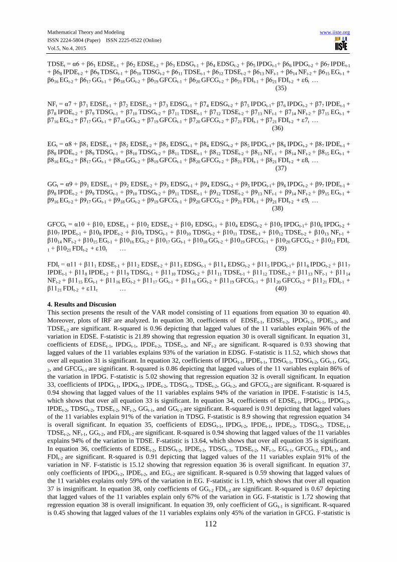
TDSEt = α6 + β61 EDSEt-1 + β62 EDSEt-2 + β63 EDSGt-1 + β64 EDSGt-2 + β65 IPDGt-1+ β66 IPDGt-2 + β67 IPDEt-1



(35)

NFt = α7 + β71 EDSEt-1 + β72 EDSEt-2 + β73 EDSGt-1 + β74 EDSGt-2 + β75 IPDGt-1+ β76 IPDGt-2 + β77 IPDEt-1 +

β78 IPDEt-2 + β79 TDSGt-1 + β710 TDSGt-2 + β711 TDSEt-1 + β712 TDSEt-2 + β713 NFt-1 + β714 NFt-2 + β715 EGt-1 +


(36)

EGt = α8 + β81 EDSEt-1 + β82 EDSEt-2 + β83 EDSGt-1 + β84 EDSGt-2 + β85 IPDGt-1+ β86 IPDGt-2 + β87 IPDEt-1 +



(37)

GGt = α9 + β91 EDSEt-1 + β92 EDSEt-2 + β93 EDSGt-1 + β94 EDSGt-2 + β95 IPDGt-1+ β96 IPDGt-2 + β97 IPDEt-1 +



(38)

GFCGt = α10 + β101 EDSEt-1 + β102 EDSEt-2 + β103 EDSGt-1 + β104 EDSGt-2 + β105 IPDGt-1+ β106 IPDGt-2 +

β107 IPDEt-1 + β108 IPDEt-2 + β109 TDSGt-1 + β1010 TDSGt-2 + β1011 TDSEt-1 + β1012 TDSEt-2 + β1013 NFt-1 +

β1014 NFt-2 + β1015 EGt-1 + β1016 EGt-2 + β1017 GGt-1 + β1018 GGt-2 + β1019 GFCGt-1 + β1020 GFCGt-2 + β1021 FDIt-

1 + β1021 FDIt-2 + 10t … (39)

FDIt = α11 + β111 EDSEt-1 + β112 EDSEt-2 + β113 EDSGt-1 + β114 EDSGt-2 + β115 IPDGt-1+ β116 IPDGt-2 + β117

IPDEt-1 + β118 IPDEt-2 + β119 TDSGt-1 + β1110 TDSGt-2 + β1111 TDSEt-1 + β1112 TDSEt-2 + β1113 NFt-1 + β1114

NFt-2 + β1115 EGt-1 + β1116 EGt-2 + β1117 GGt-1 + β1118 GGt-2 + β1119 GFCGt-1 + β1120 GFCGt-2 + β1121 FDIt-1 +

β1121 FDIt-2 + 11t … (40)

4. Results and Discusion

This section presents the result of the VAR model consisting of 11 equations from equation 30 to equation 40.

Moreover, plots of IRF are analyzed. In equation 30, coefficients of EDSEt-1, EDSEt-2, IPDGt-2, IPDEt-2, and

TDSEt-2 are significant. R-squared is 0.96 depicting that lagged values of the 11 variables explain 96% of the

variation in EDSE. F-statistic is 21.89 showing that regression equation 30 is overall significant. In equation 31,

coefficients of EDSEt-1, IPDGt-1, IPDEt-2, TDSEt-2, and NFt-2 are significant. R-squared is 0.93 showing that

lagged values of the 11 variables explains 93% of the variation in EDSG. F-statistic is 11.52, which shows that

over all equation 31 is significant. In equation 32, coefficients of IPDGt-1, IPDEt-1, TDSGt-1, TDSGt-2, GGt-1, GGt-

2, and GFCGt-1 are significant. R-squared is 0.86 depicting that lagged values of the 11 variables explain 86% of

the variation in IPDG. F-statistic is 5.02 showing that regression equation 32 is overall significant. In equation

33, coefficients of IPDGt-1, IPDGt-2, IPDEt-2, TDSGt-1, TDSEt-2, GGt-2, and GFCGt-2 are significant. R-squared is

0.94 showing that lagged values of the 11 variables explains 94% of the variation in IPDE. F-statistic is 14.5,

which shows that over all equation 33 is significant. In equation 34, coefficients of EDSEt-1, IPDGt-1, IPDGt-2,

IPDEt-2, TDSGt-2, TDSEt-2, NFt-2, GGt-1, and GGt-2 are significant. R-squared is 0.91 depicting that lagged values

of the 11 variables explain 91% of the variation in TDSG. F-statistic is 8.9 showing that regression equation 34

is overall significant. In equation 35, coefficients of EDSGt-1, IPDGt-2, IPDEt-1, IPDEt-2, TDSGt-2, TDSEt-1,

TDSEt-2, NFt-1, GGt-2, and FDIt-2 are significant. R-squared is 0.94 showing that lagged values of the 11 variables

explains 94% of the variation in TDSE. F-statistic is 13.64, which shows that over all equation 35 is significant.

In equation 36, coefficients of EDSEt-2, EDSGt-2, IPDEt-2, TDSGt-1, TDSEt-2, NFt-1, EGt-1, GFCGt-2, FDIt-1, and

FDIt-2 are significant. R-squared is 0.91 depicting that lagged values of the 11 variables explain 91% of the

variation in NF. F-statistic is 15.12 showing that regression equation 36 is overall significant. In equation 37,

only coefficients of IPDGt-2, IPDEt-2, and EGt-2 are significant. R-squared is 0.59 showing that lagged values of

the 11 variables explains only 59% of the variation in EG. F-statistic is 1.19, which shows that over all equation

37 is insignificant. In equation 38, only coefficients of GGt-2 FDIt-2 are significant. R-squared is 0.67 depicting

that lagged values of the 11 variables explain only 67% of the variation in GG. F-statistic is 1.72 showing that

regression equation 38 is overall insignificant. In equation 39, only coefficient of GGt-1 is significant. R-squared

is 0.45 showing that lagged values of the 11 variables explains only 45% of the variation in GFCG. F-statistic is




Vol.5, No.4, 2015

113

0.68, which shows that over all equation 39 is insignificant. In equation 40, coefficients of EDSEt-2 and EDSGt-2

are significant. R-squared is 0.92 depicting that lagged values of the 11 variables explain 92% of the variation in

FDI. F-statistic is 9.8 showing that regression equation 40 is overall significant. Appendix C summarizes the

output of the VAR model obtained via Eviews. According to the results of VAR model, the variables included in

this paper are suitable to predict the stock based indicators (EDSE and EDSG), flow based indicators (TDSE and

TDSG), and the cost based indicators (IPDE and IPDG) of indebtedness. Moreover, domestic capacity of

repayments of external debt (EG and GG) is unpredictable using this VAR model. However; the foreign

resources to repay external debts (NF and FDI) are predictable via the variables in the VAR model. Hence the

debt burden has no long run impact on the tow major sources of repayment of external debt in Sudan, GDP and

exports. The only resources of Sudan that are affected by the external debt are foreign resources. Hence, debt

sustainability depends on the efficient use of the foreign resources, net foreign assets and foreign direct

investments.

Analysis of shocks found significant estimates and given in the IRFs plots. Ratio of external debt to GDP is

found to be significantly related with only one foreign capacity of repayment, net foreign assets, and no domestic

capacity of repayment. Ratio of total debt servicing to GDP is found to be significantly affected by one foreign

capacity of repayment, net foreign assets, and one domestic capacity of repayment, GDP growth. Ratio of total

debt servicing to exports is found to be significantly affected by both of the foreign capacity of repayment,

foreign direct investment and net foreign assets and one domestic capacity of repayment, GDP growth. Ratio of

interest payments on external debt to exports is not significantly impacted by any foreign or domestic capacity of

repayment. Ratio of interest payment on external debt to GDP is found to be significantly affected by two

domestic capacities of repayment, GDP growth and gross fixed capital growth. the IRF plots of the above

discussed significant responses, shows that the indicators of indebtedness response negatively to the positive

shocks in the domestic capacity to repay. (appendix A-1).

Net foreign assets are found to be significantly affected by both of the stock based indicators of indebtedness,

ratio of external debt to GDP and ratio of external debt to exports. From the flow based indicators of

indebtedness, only one indicator, ratio of total debt service to GDP, significantly affect net foreign assets. One of

the cost based indicators of indebtedness, ratio of interest payment on external debt to exports, significantly

affects the net foreign assets. Net foreign assets responses positively to the shock in ratio of total debt service to

GDP and negatively to the shock in the ratio of external debt to exports. Response of net foreign assets to ratio of

external debt to GDP and ratio of interest payment on external debt to exports fluctuates around the line of zero

response. (see appendix A-2) for the above discussed significant responses. Only one domestic capacity, exports

growth, is found to be significantly affected by the cost based indicators of indebtedness, ratio of interest

payment on external debt to GDP and ratio of interest payment on external debt to exports. No other indicator of

indebtedness found to affect any other domestic capacity of repayment. Only stock based indicators of

indebtedness are found significantly affect the foreign direct investment, the foreign capacity of repayment.

Foreign direct investments have positive response to the shock in ratio of external debt to GDP and negative

response to the shock in ratio of external debt to exports. Response of exports growth to the cost based indicators

of indebtedness fluctuates around the line of zero response. (see Appendix A-3) for the above discussed

significant responses.

Sustainable levels of stock based indicators of external debt in Sudan can only be achieved by setting policies for

net foreign assets. However, flow based indicators of indebtedness can be made sustainable through improving

the domestic capacity of repayment, specifically GDP. Cost based indicators of external debt in Sudan can be

controlled to sustainable level if the gross fixed capital formation is also improved with the GDP. There is a

bidirectional relationship between net foreign assets and total debt service to GDP ratio. Thus, any policy to

make the flow based indicator of indebtedness must consider this nature of relationship. Cost based indicators of

external indebtedness are most essential to keep sustainable as they significantly impact a major source of

income of Sudan that is exports. Export growth significantly response to the shock in the interest payment on

external debt; hence, sustainable interest payments are crucial.

5. Conclusion

This paper provides with an effective model to analyze the external debt sustainability of a developing country,

taking the case of Sudan. External debt has a confusing role in the process of economic development of a

country. On one hand it is an obligation; therefore always avoided. On the other hand, it is a supplement of the




Vol.5, No.4, 2015

114

low domestic saving and hence required to finance the investments. Hence, the assessment and evaluations of the

long run impact of external debt has always been an active area of research. Only recently, the question of

dynamic association of the external indebtedness of a country and the country’s growth has been questioned.

Different methods and statistical tools are presented to assess in answering this question. One of such methods is

vector autoregressive (VAR) model followed by a sensitivity analysis of the estimates using impulse response

function (IRF). In VAR model, every variable can be considered as endogenous variables; hence, choice of

variables requires close consideration. In this paper, the variables to be inserted in the VAR model are divided

into broad categories; indicators of indebtedness and measures of repayment capacity. Indicators of indebtedness

are further classified into three categories; stock based indicators, flow based indicators, and cost based

indicators. The measures of repayment capacity are further classified as domestic capacity of repayment and

foreign capacity of repayment. A total of 11 variables are introduced to be used in the VAR mode. And hence,

11 equations are formed. Model specification in this paper is done carefully, starting from the very initial steps

of the VAR procedure using a 2-variabel 2-equation model.

Time series data is inserted in the VAR model for the period 1970-2012. The data is collected for Sudan from the

website of the World Bank, which provides World Development Indicators (WDI). Eviews is used to estimate

the model. The estimates are further used to calculate IRF for the significant relationships only. IRFs plots are

provided in this paper. The results showed that all the three indicators of indebtedness; the stock based

indicators, the flow based indicators, and the cost based indicators, are predictable using the measures of foreign

and domestic capacity to repay the external debt. In turn, the indicators of indebtedness can predict only foreign

direct investment in Sudan. No other measures of foreign and domestic capacity to repay external debt are

predictable by the indicators of indebtedness. IRF plots showed that mostly the response of all three indicators of

indebtedness is negative to the shocks in the capacity to repay external debt. The indicators of indebtedness

respond more to the shocks in the domestic capacities of repayment than to the shocks in the foreign capacity of

repayments. Effective policies to enhance the domestic capacities to repay external debt are recommended on the

basis of this result. As net foreign assets are also found to be significantly effected in turn by the indicators of

indebtedness, it is realized that the policies to control indebtedness to a sustainable level must consider its effects

on the foreign capacity of repayments. Cost based indicators of indebtedness significantly affect the exports

growth of Sudan. Hence, from the three indicators of indebtedness, interest payment on external debt is the most

deteriorating factor of unstable external debt which negatively affects the most important source of income in the

indebted country that is exports.

References

Ajayi, S. I., & Khan, M. S. (2000). External debt and capital flight in Sub-Saharan Africa. International

Monetary Fund Institute. from,

http://search.ebscohost.com/login.aspx?direct=true&scope=site&db=nlebk&db=nlabk&AN=449498

Arnone, M., Bandiera, L., & Presbitero, A. F. (2005). External Debt Sustainability Theory and Empirical

Evidenc. doi: http://128.118.178.162/eps/if/papers/0512/0512007.pdf

Chenery, H. B., & Strout, A. M. (1965). Foreign assistance and economic development. Agency for

International Development: Dept. of State, Office of Program Coordination.

Claessens, S., Detragiache, E., Kanbur, R., & Wickbam, P. (1996). Analytical Aspects of the Debt Problems of

Heavily Indebted Countries. The world Bank, Policy Research Working Paper No.1618.

Claessens, S., World, B., Africa Regional, O., Office of the Chief, E., World, B., East, A., . . . Research, D.

(1996). Analytical aspects of the debt problems of heavily-indebted poor countries. Washington, DC:

World Bank, Africa Regional Office, Office of the Chief Economist : East Asia and Pacific Regional

Office, Office of the Regional Vice President : International Monetary Fund, Research Dept.

Colaco, F. X. (1985). International capital and economic development: World Bank and Oxford University

Press.

Eaton, J. (1992). Sovereign Debt: A Primer. Washington, DC (1818 H St., N.W., Washington 20433):

International Economics Dept., World Bank.


http://search.ebscohost.com/login.aspx?direct=true&scope=site&db=nlebk&db=nlabk&AN=449498

http://128.118.178.162/eps/if/papers/0512/0512007.pdf



Vol.5, No.4, 2015

115

Edo, S. E. (2002). The External Debt Problem in Africa: A Comparative Study of Nigeria and Morocco. African

Development Review, 14(2), 221-236. doi: 10.1111/1467-8268.00052

Hunt, S. D. (2007). Economic growth: should policy focus on investment or dynamic competition? European

Business Review, 19(4), 274-291.

Iyoha, M. A. (1997). An econometric study of debt overhang, debt reduction, investment, and economic growth

in Nigeria. Ibadan, Nigeria: National Centre for Economic Management & Administration (NCEMA).

Mehran, H. (1985, 1985). External debt management. Paper presented at the International Monetary Fund;

Central Banking Department, Washington, D.C.

Sachs, J. D. (2002). Resolving the Debt Crisis of Low-Income Countries. Brookings Papers on Economic

Activity, 257-286.

Ubok-Udom, E. U. (1979). Development Through Debt: Rationalizing the Costs of External Borrowing.

Intereconomics, 14(4), 168-171.




Vol.5, No.4, 2015

116

Appendix A-1: IRF Plots for Response of Indebtedness to Repayment Capacity

-14

-12

-10

-8

-6

-4

-2

0

2

1 2 3 4 5 6 7 8 9 10

Response of EDSG to Generalized OneS.D. NF Innovation

-.6

-.4

-.2

.0

.2

1 2 3 4 5 6 7 8 9 10

Response of TDSG to NF

-.6

-.4

-.2

.0

.2

1 2 3 4 5 6 7 8 9 10

Response of TDSG to GG

Response to Generalized One S.D. Innovations

-.6

-.4

-.2

.0

.2

1 2 3 4 5 6 7 8 9 10

Response of TDSG to NF

-.6

-.4

-.2

.0

.2

1 2 3 4 5 6 7 8 9 10

Response of TDSG to GG


-6

-4

-2

0

2

1 2 3 4 5 6 7 8 9 10

Response of TDSE to NF

-6

-4

-2

0

2

1 2 3 4 5 6 7 8 9 10

Response of TDSE to GG

-6

-4

-2

0

2

1 2 3 4 5 6 7 8 9 10

Response of TDSE to FDI


-6

-4

-2

0

2

1 2 3 4 5 6 7 8 9 10


-6

-4

-2

0

2

1 2 3 4 5 6 7 8 9 10


-6

-4

-2

0

2

1 2 3 4 5 6 7 8 9 10



-6

-4

-2

0

2

1 2 3 4 5 6 7 8 9 10


-6

-4

-2

0

2

1 2 3 4 5 6 7 8 9 10


-6

-4

-2

0

2

1 2 3 4 5 6 7 8 9 10



-.4

-.3

-.2

-.1

.0

.1

1 2 3 4 5 6 7 8 9 10

Response of IPDG to GG

-.4

-.3

-.2

-.1

.0

.1

1 2 3 4 5 6 7 8 9 10

Response of IPDG to GFCG


-.4

-.3

-.2

-.1

.0

.1

1 2 3 4 5 6 7 8 9 10

Response of IPDG to GG

-.4

-.3

-.2

-.1

.0

.1

1 2 3 4 5 6 7 8 9 10

Response of IPDG to GFCG





Vol.5, No.4, 2015

117

Appendix A-2:IRF Plots for Response of Net Foreign Assets to Indebtedness

Appendix A-3: IRF Plots for Response of Repayment Capacities to Indebtedness

-800,000,000

-400,000,000

0

400,000,000

1 2 3 4 5 6 7 8 9 10

Response of NF to EDSE

-800,000,000

-400,000,000

0

400,000,000

1 2 3 4 5 6 7 8 9 10

Response of NF to EDSG

-800,000,000

-400,000,000

0

400,000,000

1 2 3 4 5 6 7 8 9 10

Response of NF to IPDE

-800,000,000

-400,000,000

0

400,000,000

1 2 3 4 5 6 7 8 9 10

Response of NF to TDSG


-6

-4

-2

0

2

4

6

1 2 3 4 5 6 7 8 9 10

Response of EG to IPDG

-6

-4

-2

0

2

4

6

1 2 3 4 5 6 7 8 9 10

Response of EG to IPDE


-400,000,000

-200,000,000

0

200,000,000

400,000,000

600,000,000

1 2 3 4 5 6 7 8 9 10

Response of FDI to EDSE

-400,000,000

-200,000,000

0

200,000,000

400,000,000

600,000,000

1 2 3 4 5 6 7 8 9 10

Response of FDI to EDSG





Vol.5, No.4, 2015

118

Appendix B: IRF Tables

Table 2.IRF for Response of EDSG to NF

Period

1 -2.933088

2 -2.559798

3 -12.42201

4 -11.90654

5 -10.42397

6 -9.010264

7 -6.102706

8 -3.562700

9 -0.572359

10 1.373697

Generalized Impulse

Table 3. IRF for Response of TDSG to NF and GG

Period NF GG

1 0.083277 -0.079764

2 0.103375 -0.202489

3 0.013443 -0.500471

4 -0.070947 -0.249628

5 -0.048390 -0.118819

6 0.035467 -0.025022

7 0.001832 0.027531

8 -0.012068 0.002622

9 0.035689 -0.035274

10 0.016050 0.063654

Generalized Impulse




Vol.5, No.4, 2015

119

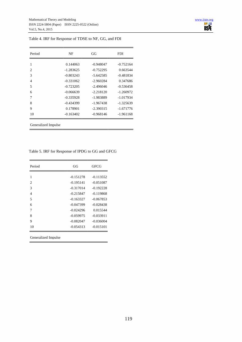
Table 4. IRF for Response of TDSE to NF, GG, and FDI

Period NF GG FDI

1 0.144063 -0.948047 -0.752164

2 -1.283625 -0.752295 0.663544

3 -0.803243 -5.642585 -0.481834

4 -0.331062 -2.960284 0.347686

5 -0.723205 -2.496046 -0.536458

6 -0.066639 -2.218120 -1.260972

7 -0.335928 -1.983889 -1.017934

8 -0.434399 -1.967438 -1.325639

9 0.178901 -2.390315 -1.671776

10 -0.163402 -0.968146 -1.961168

Generalized Impulse

Table 5. IRF for Response of IPDG to GG and GFCG

Period GG GFCG

1 -0.151278 -0.113552

2 -0.195141 -0.051087

3 -0.317014 -0.192228

4 -0.215847 -0.119868

5 -0.163327 -0.067853

6 -0.047399 -0.028438

7 -0.024296 0.015544

8 -0.059975 -0.033911

9 -0.082047 -0.036004

10 -0.054313 -0.015101

Generalized Impulse




Vol.5, No.4, 2015

120

Table 6. IRF for Response of NF to EDSE, EDSG, IPDE, and TDSG

Period EDSE EDSG IPDE TDSG

1 -1.85E+08 -1.05E+08 -74989774 1.63E+08

2 -4.08E+08 1.23E+08 -1.08E+08 5.39E+08

3 -6.19E+08 1.36E+08 56128676 4.37E+08

4 -4.04E+08 -1.34E+08 1.66E+08 3.81E+08

5 -4.23E+08 -40342046 2.13E+08 2.42E+08

6 -3.68E+08 -1.36E+08 2.69E+08 1.18E+08

7 -3.36E+08 -98433332 2.78E+08 21302867

8 -3.39E+08 -67180235 3.16E+08 -9756689.

9 -3.74E+08 32780422 2.52E+08 58587592

10 -3.93E+08 1.15E+08 1.54E+08 1.69E+08

Generalized Impulse

Table 7.IRF for Response of EG to IPDE and IPDG

Period IPDE IPDG

1 -4.816459 4.261872

2 3.425221 -1.344313

3 1.785196 -1.241352

4 -2.328804 1.359812

5 -4.325722 -0.610222

6 -2.235729 -2.447994

7 -1.573983 -2.432179

8 -3.267538 -2.438304

9 -3.102953 -2.839058

10 -3.118011 -3.612517

Generalized Impulse




Vol.5, No.4, 2015

121

Table 8. IRF for Response of FDI to EDSE and EDSG

Period EDSE EDSG

1 -1.82E+08 1.04E+08

2 -2.37E+08 2.30E+08

3 -3.75E+08 3.93E+08

4 -3.35E+08 2.85E+08

5 -3.93E+08 3.96E+08

6 -3.45E+08 3.12E+08

7 -2.82E+08 3.07E+08

8 -2.30E+08 2.83E+08

9 -1.85E+08 2.71E+08

10 -1.48E+08 2.58E+08

Generalized Impulse




Vol.5, No.4, 2015

122

Appendix C: Estimation of VAR Model

EDSE EDSG IPDG IPDE TDSG TDSE NF EG GG GFCG FDI

EDSE(-1) 1.056670* 0.040760* -4.87E-05 0.000228 -0.00041*** -0.002660 314276.0 -0.006380 0.000233 0.002293 -67767.47

(0.21550) (0.01331) (0.00019) (0.00128) (0.00024) (0.00204) (474296.) (0.01419) (0.00267) (0.01570) (494409.)

[ 4.90330] [ 3.06265] [-0.25721] [ 0.17822] [-1.68932] [-1.30182] [ 0.66262] [-0.44948] [ 0.08736] [ 0.14609] [-0.13707]

EDSE(-2) -0.4757** -0.009456 0.000186 0.000320 0.000354 0.000638 -1379046*. 0.007543 0.000937 0.000180

-

966262.1***

(0.22044) (0.01361) (0.00019) (0.00131) (0.00025) (0.00209) (485164.) (0.01452) (0.00273) (0.01606) (505737.)

[-2.15804] [-0.69463] [ 0.95952] [ 0.24478] [ 1.42666] [ 0.30549] [-2.84243] [ 0.51947] [ 0.34357] [ 0.01120] [-1.91060]

EDSG(-1) 2.290466 0.137556 -0.003324 -0.031364 -0.005061 -0.0707*** 6762332. -0.011026 -0.016638 -0.010763 2539585.

(3.86159) (0.23848) (0.00339) (0.02288) (0.00434) (0.03661) (8498934) (0.25435) (0.04779) (0.28126) (8859329)

[ 0.59314] [ 0.57681] [-0.98016] [-1.37051] [-1.16555] [-1.93206] [ 0.79567] [-0.04335] [-0.34814] [-0.03827] [ 0.28666]

EDSG(-2) -4.399345 -0.336369 0.000406 0.017500 -0.000787 0.034315

13386454*** 0.014368 0.031739 -0.070304

13518323***

(3.46932) (0.21425) (0.00305) (0.02056) (0.00390) (0.03289) (7635599) (0.22851) (0.04294) (0.25269) (7959384)

[-1.26807] [-1.56996] [ 0.13313] [ 0.85116] [-0.20186] [ 1.04336] [ 1.75316] [ 0.06287] [ 0.73922] [-0.27823] [ 1.69841]

IPDG(-1) 313.1070

60.21163*** 1.911709* 6.754640** 1.628288* -2.515399 -1.19E+09 5.853567 -2.257136 62.57066 58130028

(573.243) (35.4015) (0.50342) (3.39718) (0.64457) (5.43428) (1.3E+09) (37.7575) (7.09442) (41.7518) (1.3E+09)

[ 0.54620] [ 1.70082] [ 3.79744] [ 1.98831] [ 2.52617] [-0.46288] [-0.94646] [ 0.15503] [-0.31816] [ 1.49863] [ 0.04420]

IPDG(-2) -1040*** -24.75649 -0.182941

5.864633*** 1.121057*** 16.35717* -1.60E+09 71.59720*** -4.825779 -2.590208 -6.79E+08

(589.333) (36.3952) (0.51755) (3.49253) (0.66266) (5.58681) (1.3E+09) (38.8173) (7.29354) (42.9236) (1.4E+09)

[-1.76449] [-0.68021] [-0.35348] [ 1.67919] [ 1.69176] [ 2.92782] [-1.23058] [ 1.84447] [-0.66165] [-0.06034] [-0.50206]

IPDE(-1) 32.01167 -2.262018 -0.126890* 0.067206 -0.082127 2.105018* 1.62E+08 -1.017541 1.017824 -2.014312 52716860

(63.1559) (3.90029) (0.05546) (0.37428) (0.07101) (0.59871) (1.4E+08) (4.15985) (0.78161) (4.59992) (1.4E+08)

[ 0.50687] [-0.57996] [-2.28782] [ 0.17956] [-1.15649] [ 3.51592] [ 1.16830] [-0.24461] [ 1.30221] [-0.43790] [ 0.36383]

IPDE(-2)

219.3322* 7.221339** -0.058492 -0.926206* -0.233121* -2.321273* 2.11E+08*** -8.312801** -0.715766 -1.295137 54516129

(55.8095) (3.44661) (0.04901) (0.33074) (0.06275) (0.52907) (1.2E+08) (3.67598) (0.69069) (4.06485) (1.3E+08)

[ 3.93001] [ 2.09520] [-1.19343] [-2.80040] [-3.71488] [-4.38747] [ 1.71582] [-2.26139] [-1.03630] [-0.31862] [ 0.42578]

TDSG(-1) -186.5081 -18.95530 -0.54489** -3.595561** -0.376062 -3.324137 1.01E+09*** -12.48302 -0.162171 -18.54237 -2.35E+08

(277.954) (17.1655) (0.24410) (1.64722) (0.31254) (2.63497) (6.1E+08) (18.3078) (3.43994) (20.2446) (6.4E+08)

[-0.67100] [-1.10427] [-2.23226] [-2.18281] [-1.20326] [-1.26155] [ 1.65415] [-0.68184] [-0.04714] [-0.91592] [-0.36902]

TDSG(-2) 137.2569 2.612896 0.002895 -1.456363 -0.466113** -3.58143** 2.84E+08 -17.51029 2.606192 0.428720 -93026420

(196.494) (12.1348) (0.17256) (1.16447) (0.22094) (1.86275) (4.3E+08) (12.9424) (2.43180) (14.3115) (4.5E+08)

[ 0.69853] [ 0.21532] [ 0.01678] [-1.25066] [-2.10966] [-1.92266] [ 0.65587] [-1.35294] [ 1.07171] [ 0.02996] [-0.20636]

TDSE(-1) -43.09904 -1.567581

0.059637** 0.190027 0.032678 -0.5222*** -1.02E+08 1.065946 0.066241 0.790385 -26354550

(30.7863) (1.90125) (0.02704) (0.18245) (0.03462) (0.29185) (6.8E+07) (2.02778) (0.38101) (2.24229) (7.1E+07)

[-1.39994] [-0.82450] [ 2.20580] [ 1.04155] [ 0.94400] [-1.78957] [-1.50164] [ 0.52567] [ 0.17386] [ 0.35249] [-0.37313]

TDSE(-2) -101.107* -4.009099*

0.047776** 0.653775* 0.108881* 0.942242* -51887450 2.479884 -0.159016 -0.744782 -24692831

(24.8718) (1.53599) (0.02184) (0.14740) (0.02797) (0.23578) (5.5E+07) (1.63821) (0.30781) (1.81152) (5.7E+07)

[-4.06512] [-2.61010] [ 2.18730] [ 4.43550] [ 3.89330] [ 3.99625] [-0.94789] [ 1.51377] [-0.51660] [-0.41114] [-0.43274]

NF(-1) 1.22E-08 4.92E-09 6.34E-11 -2.98E-10 1.33E-10

-1.3E-

10*** 1.094788* -6.33E-10 4.28E-10 -2.89E-10 0.126779

(8.6E-08) (5.3E-09) (7.6E-11) (5.1E-10) (9.7E-11) (8.2E-10) (0.19002) (5.7E-09) (1.1E-09) (6.3E-09) (0.19808)

[ 0.14077] [ 0.92320] [ 0.83611] [-0.58327] [ 1.36805] [-1.63533] [ 5.76134] [-0.11123] [ 0.40090] [-0.04597] [ 0.64004]

NF(-2) -3.92E-08 -1.38E-08* -2.43E-11 3.76E-10 -1.77E-10*** 2.75E-10 -0.154876 -6.29E-09 -7.22E-10 -3.13E-09 0.107583

(8.7E-08) (5.4E-09) (7.7E-11) (5.2E-10) (9.8E-11) (8.3E-10) (0.19233) (5.8E-09) (1.1E-09) (6.4E-09) (0.20048)

[-0.44821] [-2.56155] [-0.31639] [ 0.72559] [-1.79868] [ 0.33230] [-0.80527] [-1.09270] [-0.66746] [-0.49226] [ 0.53661]

EG(-1) -0.190809 0.125732 0.003479 0.022138 0.003847 0.004937 25393527* -0.158093 0.003307 -0.137267 13882447

(3.96194) (0.24468) (0.00348) (0.02348) (0.00445) (0.03756) (8719798) (0.26096) (0.04903) (0.28856) (9089558)

[-0.04816] [ 0.51387] [ 1.00000] [ 0.94285] [ 0.86346] [ 0.13144] [ 2.91217] [-0.60582] [ 0.06745] [-0.47569] [ 1.52730]

EG(-2) 2.902134 -0.013827 0.001810 0.019673 -0.006072 -0.020693 -8379088. -0.530060** -0.047813 -0.141263 -1911732.

(3.95389) (0.24418) (0.00347) (0.02343) (0.00445) (0.03748) (8702088) (0.26043) (0.04893) (0.28798) (9071098)

[ 0.73399] [-0.05663] [ 0.52116] [ 0.83958] [-1.36583] [-0.55207] [-0.96288] [-2.03534] [-0.97712] [-0.49053] [-0.21075]

GG(-1) 5.844489 0.352099 -0.03666** -0.065790 -0.023196 0.157629 36023519 0.693610 0.116491 2.4768*** 44489119

(19.6376) (1.21275) (0.01725) (0.11638) (0.02208) (0.18616) (4.3E+07) (1.29346) (0.24303) (1.43029) (4.5E+07)

[ 0.29762] [ 0.29033] [-2.12554] [-0.56532] [-1.05050] [ 0.84673] [ 0.83349] [ 0.53624] [ 0.47932] [ 1.73167] [ 0.98748]




Vol.5, No.4, 2015

123

GG(-2) -17.24666 -1.016562 -0.03097** -0.327160* -0.058488* -0.871464* 74796373** -0.487869 -0.38524** -0.313175 28516595

(18.0366) (1.11388) (0.01584) (0.10689) (0.02028) (0.17099) (4.0E+07) (1.18801) (0.22322) (1.31369) (4.1E+07)

[-0.95620] [-0.91263] [-1.95546] [-3.06074] [-2.88392] [-5.09672] [ 1.88420] [-0.41066] [-1.72583] [-0.23839] [ 0.68914]

GFCG(-1) 3.866376 0.204108

0.009079** 0.021193 0.006518 0.000535 -12971079 -0.322686 0.065374 -0.190544 -698446.1

(4.86085) (0.30019) (0.00427) (0.02881) (0.00547) (0.04608) (1.1E+07) (0.32017) (0.06016) (0.35404) (1.1E+07)

[ 0.79541] [ 0.67993] [ 2.12695] [ 0.73571] [ 1.19246] [ 0.01161] [-1.21245] [-1.00787] [ 1.08671] [-0.53821] [-0.06263]

GFCG(-2) 0.749720 0.199553 -0.000518 -0.03610*** 0.000941 -0.024613 -16143080** 0.041027 -0.034572 -0.137490 802131.4

(3.59604) (0.22208) (0.00316) (0.02131) (0.00404) (0.03409) (7914487) (0.23686) (0.04450) (0.26191) (8250099)

[ 0.20849] [ 0.89857] [-0.16397] [-1.69388] [ 0.23278] [-0.72200] [-2.03969] [ 0.17321] [-0.77681] [-0.52494] [ 0.09723]

FDI(-1) -6.51E-08 -9.36E-10 -9.53E-12 3.71E-10 -8.01E-11 9.93E-10 -0.842111* 1.09E-08

2.68E-

09** 5.60E-09 0.326547

(1.0E-07) (6.5E-09) (9.2E-11) (6.2E-10) (1.2E-10) (9.9E-10) (0.23014) (6.9E-09) (1.3E-09) (7.6E-09) (0.23989)

[-0.62232] [-0.14489] [-0.10378] [ 0.59874] [-0.68123] [ 1.00200] [-3.65919] [ 1.58053] [ 2.07329] [ 0.73509] [ 1.36121]

FDI(-2) -1.28E-07 -5.43E-09 3.82E-11 -2.10E-10 5.71E-11 -2.45E-09* 0.716865* -6.33E-09 -1.84E-09 -5.44E-09 0.345706

(1.0E-07) (6.2E-09) (8.8E-11) (5.9E-10) (1.1E-10) (9.5E-10) (0.22074) (6.6E-09) (1.2E-09) (7.3E-09) (0.23010)

[-1.28047] [-0.87613] [ 0.43350] [-0.35326] [ 0.50659] [-2.57544] [ 3.24757] [-0.95823] [-1.47882] [-0.74535] [ 1.50242]

C

1814.489* 115.3306* 0.231026 1.288358 1.809094* 19.81522* -1.05E+09 5.714927 1.003658 16.62889 1.01E+09

(573.126) (35.3943) (0.50332) (3.39648) (0.64444) (5.43317) (1.3E+09) (37.7498) (7.09297) (41.7432) (1.3E+09)

[ 3.16595] [ 3.25845] [ 0.45901] [ 0.37932] [ 2.80725] [ 3.64708] [-0.83319] [ 0.15139] [ 0.14150] [ 0.39836] [ 0.77088]

R-squared 0.963973 0.933701 0.860627 0.946691 0.915925 0.943439 0.948672 0.594147 0.678712 0.456064 0.923507

Adj. R-

squared 0.919941 0.852668 0.690282 0.881536 0.813166 0.874310 0.885937 0.098105 0.286026 -0.208746 0.830015

Sum sq.

resids 2118316. 8078.991 1.633706 74.39589 2.678240 190.3695 1.03E+19 9190.078 324.4490 11237.32 1.11E+19

S.E. equation 343.0514 21.18568 0.301266 2.033004 0.385734 3.252089 7.55E+08 22.59557 4.245580 24.98590 7.87E+08

F-statistic 21.89235 11.52253 5.052268 14.52976 8.913377 13.64741 15.12197 1.197776 1.728385 0.686007 9.877926


The IISTE is a pioneer in the Open-Access hosting service and academic event management.

The aim of the firm is Accelerating Global Knowledge Sharing.

More information about the firm can be found on the homepage:

http://www.iiste.org

CALL FOR JOURNAL PAPERS

There are more than 30 peer-reviewed academic journals hosted under the hosting platform.

Prospective authors of journals can find the submission instruction on the following

page: http://www.iiste.org/journals/ All the journals articles are available online to the

readers all over the world without financial, legal, or technical barriers other than those

inseparable from gaining access to the internet itself. Paper version of the journals is also

available upon request of readers and authors.

MORE RESOURCES

Book publication information: http://www.iiste.org/book/

Academic conference: http://www.iiste.org/conference/upcoming-conferences-call-for-paper/

IISTE Knowledge Sharing Partners

EBSCO, Index Copernicus, Ulrich's Periodicals Directory, JournalTOCS, PKP Open

Archives Harvester, Bielefeld Academic Search Engine, Elektronische Zeitschriftenbibliothek

EZB, Open J-Gate, OCLC WorldCat, Universe Digtial Library , NewJour, Google Scholar


http://www.iiste.org/journals/

http://www.iiste.org/book/

http://www.iiste.org/conference/upcoming-conferences-call-for-paper/

Documents

Analyzing The Dynamic Nature Of The Economic Factors