Analyzing ICAT Data

Gary Van DomselaarUniversity of Alberta

Analyzing ICAT Data• ICAT: Isotope Coded Affinity Tag

• Introduced in 1999 by Ruedi Aebersold as a method for quantitative analysis of complex protein mixtures– Steven P. Gygi, Beate Rist, Scott A. Gerber,

Frantisek Turecek, Michael H. Gelb, Ruedi Aebersold (1999) Nature Biotechnology 17, 994 - 999.

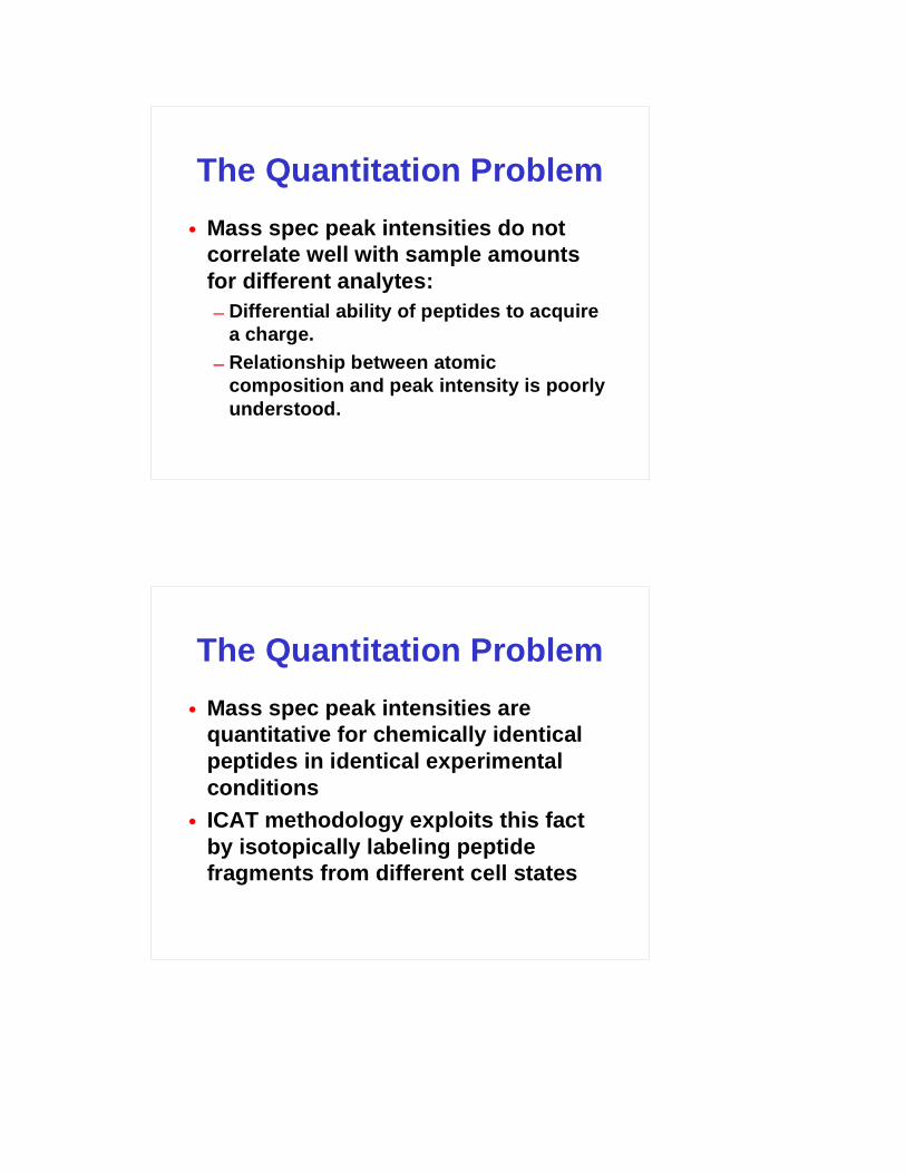
The Quantitation Problem

• Mass spec peak intensities do not correlate well with sample amounts for different analytes:– Differential ability of peptides to acquire

a charge.

– Relationship between atomic composition and peak intensity is poorly understood.

The Quantitation Problem

• Mass spec peak intensities are quantitative for chemically identical peptides in identical experimental conditions

• ICAT methodology exploits this fact by isotopically labeling peptide fragments from different cell states

The ICAT Strategy

Quantitating ICAT Peaks

Quantitating ICAT Peaks

Identifying ICAT Peaks

Identifying ICAT Peaks

ICAT Quantitation Software

• ProICAT – ABI

• SpectrumMill – Agilent

• XPRESS – Institute for Systems Biology

• ASAPRatio – Institute for Systems Biology

• XPRESS and ASAPRatio Work with Peptide Prophet and Protein Prophet

ICAT Quantitation Software

• Sashimi: free open source tools for downstream analysis of mass spectrometric data– Glossolalia: a common file format for MS

Data

– XPRESS & ASAPRatio – Foor relative quantification of isotopically labeled peptides

• http://sashimi.sourceforge.net

Goal of ICAT

• To identify changes in expression– How do we know if the changes we see

are significant?

• To correlate the changes with biochemical processes– What underlies the changes that we see?

ICAT and GeneChip Comparison

A Real Example

Meehan and Sadar Proteomics 2004, 4, 1116–1134

A Real Example

Meehan and Sadar Proteomics 2004, 4, 1116–1134

A Real Example

A Real Example

A Real Example

Scatter Plots

• Simplest kind of data plot (data scattered over a two-axis plot)

• No assumed connectivity (no lines connecting the dots)

• Challenge is to fit a line or a curve to the raw data to reveal a “trend”

A Scatter Plot

Light

Hea

vy

Correlation

“+” correlation Uncorrelated “-” correlation

Correlation

Highcorrelation

Lowcorrelation

Perfectcorrelation

Correlation Coefficient

r = 0.85 r = 0.4 r = 1.0

r = Σ(x i - µ x)(y i - µ y)

Σ(x i - µ x)2(y i - µ y)2

Correlation Coefficient

• Sometimes called coefficient of linear correlation or Pearson product-moment correlation coefficient

• A quantitative way of determining what model (or equation or type of line) best fits a set of data

• Commonly used to assess most kinds of predictions or simulations

Correlation and Outliers

Experimental error orsomething important?

A single “bad” point can destroy a good correlation

Outliers

• Can be both “good” and “bad”

• When modeling data -- you don’t like to see outliers (suggests the model is bad)

• Often a good indicator of experimental or measurement errors -- only you can know!

• When plotting ICAT data you do like to see outliers

• A good indicator of something significant

Cross Sectioning a Scatter Plot

What kind of point scatter do you see?

Gaussian or Normal Distribution

Features of a Normal Distribution

µ = mean• Symmetric Distribution

• Has an average or mean value (µ ) at the centre

• Has a characteristic width called the standard deviation (σ)

• Most common type of distribution known

Gaussian Distribution

µ - 2 σ µ - σ µ µ + σµ - 3 σ µ + 2 σ µ + 3 σ

2

2

2

)(

2

1)( σ

µ

πσ

−−=

x

exP

Some Equations

Mean µ = Σx i

N

Variance σ2 = Σ(x i - µ )2

Standard Deviation σ = Σ(x i - µ )2

N

N

Standard Deviations (Z-values)

µ ± 1.0 S.D. 0.683 > µ + 1.0 S.D. 0.158

µ ± 2.0 S.D. 0.954 > µ + 2.0 S.D. 0.023

µ ± 3.0 S.D. 0.9972 > µ + 3.0 S.D. 0.0014

µ ± 4.0 S.D. 0.99994 > µ + 4.0 S.D. 0.00003

µ ± 5.0 S.D. 0.999998 > µ + 5.0 S.D. 0.000001

µ - 2 σ µ - σ µ µ + σµ - 3 σ µ + 2 σ µ + 3 σ

2

2

2

)(

2

1)( σ

µ

πσ

−−=

x

exP

Significance & Z-values

• Generally if something is more than 2 SD away from the mean, then it is considered significant (p > 0.95)

• Sometimes used to detect “signals” from “noise” or unusual from normal

• Gene expression levels that are 2-2.5 SD above mean are often considered significant

Mean, Median & Mode

ModeMedian

Mean

Log Transformationlinear scale log2 scale

ch1 intensity0

10000

20000

30000

40000

50000

60000

70000

0 10000 20000 30000 40000 50000 60000 70000

ICA

T h

eavy

inte

nsity exp’t Aexp’t A

0

2

4

6

8

10

12

14

16

18

0 5 10 15ICAT Light intensity

Choice of Base is Not Important

0

1

2

3

4

5

6

0 2 4 6

0

2

4

6

8

10

12

14

0 5 10 15

log10 ln

exp’t Aexp’t A

Why Log2 Transformation?

• Makes variation of intensities and ratios of intensities more independent of absolute magnitude

• Makes normalization additive

• Evens out highly skewed distributions

• Gives more realistic sense of variation

• Approximates normal distribution

• Treats increased and diminished expression equally.

log2 H area lo

g 2 L

Are

a 16

16

0

Applying a log transformation makes the variance and offset more proportionate along the entire graph

H L H/L

60 000 40 000 1.5

3000 2000 1.5

log 2 H log 2 L log 2 ratio

15.87 15.29 0.58

11.55 10.97 0.58

Log Transformations

Log Transformations

Signal-to-noise

Significant?

Detecting Clusters

Weight

Hei

gh

t

Is it Right to Calculate a Correlation Coefficient?

Weight

Hei

gh

t

r = 0.73

Or is There More to This?

Weight

Hei

gh

t

Girl

Boy

Clustering Applications in Bioinformatics

• 2D Gel or ProteinChip Analysis

• Microarray or GeneChip Analysis

• Protein Interaction Analysis

• Phylogenetic and Evolutionary Analysis

• Structural Classification of Proteins

• Protein Sequence Families

• ICAT :-)

Clustering

• Definition - a process by which objects that are logically similar in characteristics are grouped together.

• Clustering is different than Classification

• In classification the objects are assigned to pre-defined classes, in clustering the classes are yet to be defined

• Clustering helps in classification

Clustering Requires...

• A method to measure similarity (a similarity matrix) or dissimilarity (a dissimilarity coefficient) between objects

• A threshold value with which to decide whether an object belongs with a cluster

• A way of measuring the “distance” between two clusters

• A cluster seed (an object to begin the clustering process)

Clustering Algorithms

• K-means or Partitioning Methods - divides a set of N objects into M clusters -- with or without overlap

• Hierarchical Methods - produces a set of nested clusters in which each pair of objects is progressively nested into a larger cluster until only one cluster remains

• Self-Organizing Feature Maps - produces a cluster set through iterative “training”

K-means or Partitioning Methods

• Make the first object the centroid for the first cluster

• For the next object calculate the similarity to each existing centroid

• If the similarity is greater than a threshold add the object to the existing cluster and redetermine the centroid, else use the object to start new cluster

• Return to step 2 and repeat until done

K-means or Partitioning Methods

Rule: λ T = λ centroid + 50 nm-

Initial cluster choose 1 choose 2 test & join centroid= centroid=

Hierarchical Clustering

• Find the two closest objects and merge them into a cluster

• Find and merge the next two closest objects (or an object and a cluster, or two clusters) using some similarity measure and a predefined threshold

• If more than one cluster remains return to step 2 until finished

Hierarchical Clustering

Rule: λ T = λ obs + 50 nm-

Initial cluster pairwise select select compare closest next closest

Hierarchical Clustering

Find 2 mostsimilar proteinexpress levelsor curves

Find the nextclosest pairof levels orcurves

Iterate

A

B

B

A

C

A

B

C

D

E

F

Self-Organizing Feature Maps

T=0

T=20 h

T=0

T=3daysT=2days

T=1day

SvOutPlaceObject

Self-Organizing Feature Maps

Cluster 1 Cluster 2

Cluster 4Cluster 3

Cluster 6Cluster 5

Plot Chip Data Compute Feature Examine Clusters forMap with 6 nodes Biological Meaning

SOMs - Details

Specify the number of nodes (clusters) desired, andSpecify the number of nodes (clusters) desired, anda 2-D geometry for the nodes (rectangular or hexagonal)a 2-D geometry for the nodes (rectangular or hexagonal)

N = NodesN = NodesG = GenesG = GenesG1G1 G6G6

G3G3

G5G5G4G4

G2G2

G11G11

G7G7G8G8

G10G10G9G9

G12G12 G13G13G14G14

G15G15

G19G19G17G17

G22G22

G18G18G20G20

G16G16

G21G21G23G23

G25G25G24G24

G26G26 G27G27

G29G29G28G28

N1N1 N2N2

N3N3 N4N4

N5N5 N6N6

Choose a random protein, e.g., G9

G1G1 G6G6

G3G3

G5G5G4G4

G2G2

G11G11

G7G7G8G8

G10G10G9G9

G12G12 G13G13G14G14

G15G15

G19G19G17G17

G22G22

G18G18

G20G20

G16G16

G21G21G23G23

G25G25G24G24

G26G26 G27G27

G29G29G28G28

N1N1 N2N2

N3N3 N4N4

N5N5 N6N6

SOMs - Details

Move the nodes in the direction of G9. The node Move the nodes in the direction of G9. The node closest to G9 (N2) is moved the most, and the other closest to G9 (N2) is moved the most, and the other nodes are moved by smaller varying amounts. The nodes are moved by smaller varying amounts. The farther away the node is from N2, the less it is moved.farther away the node is from N2, the less it is moved.

G1G1 G6G6

G3G3

G5G5G4G4

G2G2

G11G11

G7G7G8G8

G10G10G9G9

G12G12 G13G13G14G14

G15G15

G19G19G17G17

G22G22

G18G18G20G20

G16G16

G21G21G23G23

G25G25G24G24

G26G26 G27G27

G29G29G28G28

N1N1 N2N2

N3N3 N4N4

N5N5 N6N6

SOMs - Details

Repeat the process many (usually several thousand) Repeat the process many (usually several thousand) times choosing different proteins. With each iteration, times choosing different proteins. With each iteration, the amount that the nodes move is decreased.the amount that the nodes move is decreased.

G1G1 G6G6

G3G3

G5G5G4G4

G2G2

G11G11

G7G7G8G8

G10G10G9G9

G12G12 G13G13G14G14

G15G15

G19G19G17G17

G22G22

G18G18G20G20

G16G16

G21G21G23G23

G25G25G24G24

G26G26 G27G27

G29G29G28G28

N1N1N2N2

N3N3 N4N4

N5N5 N6N6

SOMs - Details

Finally, each node will “nestle” among a cluster of Finally, each node will “nestle” among a cluster of genes, and a protein will be considered to be in the genes, and a protein will be considered to be in the cluster if its distance to the node in that cluster is less cluster if its distance to the node in that cluster is less than its distance to any other node. than its distance to any other node.

SOMs - Details

G1G1 G6G6

G3G3

G5G5G4G4

G2G2

G11G11

G7G7G8G8

G10G10G9G9N1N1 N2N2

G12G12 G13G13G14G14

G15G15G26G26 G27G27

G29G29G28G28N3N3

N4N4

G19G19G17G17

G22G22

G18G18G20G20

G16G16

G21G21G23G23

G25G25G24G24N5N5

N6N6

–Excel

–MATLAB

–Octave

–SAS

–SPSS

–S-PLUS

–Statistica

–R

Statistics Software

Cluster Annotation• Once you have your clusters, annotate them and look for

patterns that can reveal the underlying process

– Metabolism:

• KEGG

– http://www.genome.ad.jp/kegg/metabolism.html

• Roche/Boeringer

– http://www.expasy.org/cgi-bin/search-biochem-index

• EcoCyc

– www.ecocyc.org

• PathDB

– http://www.ncgr.org/pathdb

Cluster Annotation• Interaction Databases

– BIND

• http://www.bind.ca

– DIP

• http://dip.doe-mbi.ucla.edu/

– MINT• http://mint.bio.uniroma2.it/mint

– PathCalling

• http://protal.curagen.com/extpc/com.curagen.portal.servlet.Yeast

Cluster Annotation• Bibliographic Databases

– PubMed Medline

• http://www.ncbi.nlm.nih.gov/PubMed/

– Science Citation Index

• http://isi4.isiknowledge.com/portal.cgi

– Your Local Library• www.XXXX.ca

– Current Contents

• http://www.isinet.com/isi

Cluster Annotation• Other

– SWISSPROT: Curated Expert Annotations

• http://www.expasy.org/

– Subcellular Localization

• http://www.cs.ualberta.ca/~bioinfo/PA/Sub/

– Genome Ontology• http://www.geneontology.org/