Analytically computed rates of seepage flow into drains and cavities

Correspondence to: A. R. Kacimov, Institute of Mathematics and Mechanics, Kazan University, 17, University Str., 42008Kazan, Russia

CCC 0363—9061/98/040277—25$17.50 Received 17 March 1997( 1998 John Wiley & Sons, Ltd. Revised 16 July 1997

INTERNATIONAL JOURNAL FOR NUMERICAL AND ANALYTICAL METHODS IN GEOMECHANICS, VOL. 22, 277—301 (1998)

ANALYTICALLY COMPUTED RATES OF SEEPAGE FLOWINTO DRAINS AND CAVITIES

N. FUJII1 AND A. R. KACIMOV2*

1 Osaka Sangyo University, Osaka, Japan2 Institute of Mathematics & Mechanics, Kazan University, 17, University Str., 420008, Kazan, Russia

SUMMARY

The known formulae of Freeze and Cherry, Polubarinova—Kochina, Vedernikov for flow rate during 2-Dseepage into horizontal drains and axisymmetric flow into cavities are examined and generalized. The case ofan empty drain under ponded soil surface is studied and existence of drain depth providing minimal seepagerate is presented. The depth is found exhibiting maximal difference in rate between a filled and an emptydrain. 3-D flow to an empty semi-spherical cavity on an impervious bottom is analysed and the difference inrate as compared with a completely filled cavity is established. Rate values for slot drains in a two-layeraquifer are ‘inverted’ using the Schulgasser theorem from the Polubarinova—Kochina expressions forcorresponding flow rates under a dam. Flow to a point sink modelling a semi-circular drain in a layeredaquifer is treated by the Fourier transform method. For unsaturated flow the catchment area of a singledrain is established in terms of the quasi-linear model assuming the isobaric boundary condition along thedrain contour. Optimal shape design problems for irrigation cavities are addressed in the class of arbitrarycontours with seepage rate as a criterion and cavity cross-sectional area as an isoperimetric restriction.( 1997 John Wiley & Sons, Ltd.

Int. J. Numer. Anal. Meth. Geomech., Vol. 22, 277—301 (1998)

Key words: seepage; flow rate; drain; tunnel; optimization

1. INTRODUCTION

Drains, openings, tunnels or natural cavities are either designed for purposive seepage or areinfluenced by undesirable subsurface flows in their vicinity. In any case, accurate prediction oftotal volume of seeping water and hydraulic gradients is important. Standard software may fail toreproduce these characteristics in a ‘fine scale’ and analytic expressions can be useful.

With the advent of FDM—FEM packages analytic solutions for seepage flow problems becamea supplementary tool in engineering practice. However, new environment like Mathematicaallows one to reconsider applicability of ‘old-fashioned’ analytic technique which restores fromseemingly ponderous forms into standard built-in computer operations. In this paper, we studyanalytically seepage into horizontal drains and cavities. Our goal is both to fill in the lacunae inthe classical books1~5 — and to derive some new solutions. We focus our interest on one of themost important characteristics, total rate of water seeping into a drain, even though other

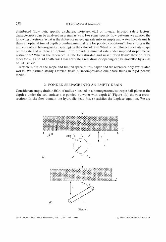
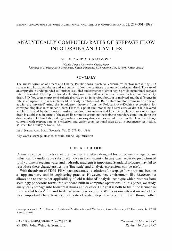
Figure 1

distributed (flow nets, specific discharge, moisture, etc.) or integral (erosion safety factors)characteristics can be analysed in a similar way. For some specific flow patterns we answer thefollowing questions: What is the difference in seepage rate into an empty and water filled drain? Isthere an optimal tunnel depth providing minimal rate for ponded conditions? How strong is theinfluence of soil heterogeneity (layering) on the value of rate? What is the influence of cavity shapeon the rate and is there an optimal form providing minimal rate under imposed isoperimetricrestrictions? What is the difference in rate for saturated and unsaturated flows? How do ratesdiffer for 2-D and 3-D patterns? How accurate a real drain or opening can be modelled by a 2-Dor 3-D sinks?

Review is out of the scope and limited space of this paper and we reference only few relatedworks. We assume steady Darcian flows of incompressible one-phase fluids in rigid porousmedia.

2. PONDED SEEPAGE INTO AN EMPTY DRAIN

Consider an empty drain ABCA of radius r located in a homogeneous, isotropic half-plane at thedepth c under the soil surface a—a ponded by water with depth H (Figure 1(a) shows a cross-section). In the flow domain the hydraulic head h(x, y) satisfies the Laplace equation. We are

278 N. FUJII AND A. R. KACIMOV

( 1998 John Wiley & Sons, Ltd.Int. J. Numer. Anal. Meth. Geomech., Vol. 22, 277—301 (1998)

interested in the value of total seepage rate q%into the drain and its difference from the rate q

&of

a drain filled with water.The case of a filled drain is described everywhere and the formula obtained by Forchheimer2 in

1889 states

q&"

2n*H

arc cosh(c/r )(1)

where *H is the head difference between a—a and the drain contour. Polubarinova-Kochina4(p. 354) gives an approximate formula q

&"2n*H/ln (2c/r). Here and below for saturated

homogeneous matrixes we normalize / and q to hydraulic conductivity k. Note, thatPolubarinova-Kochina reproduced only an approximation of the exact formula of Vedernikov5,who repeated the formula of Forchheimer.

For the sake of further comparison with empty drains restrict ourselves (without any loss ofgenerality) with the limiting case when the pressure p (divided by the specific weight of water) atthe point A (drain top) is atmospheric (zero), i.e. *H"H!y

A. Thorough explanation of

boundary conditions along a drain contour is given by Khan and Rushton.6Forchheimer modelled the drain (well) by a point sink placed at the depth d"c tanh(2n*H/q

&).

Note that the Forchheimer drain contour (an equipotential of the corresponding sink) is exactlya circle while for all other flow patterns1,5 equipotentials deviate from circles.

For the case of empty drain (tunnel) Freeze and Cherry3 say (p. 490, equation (10.17) that theonly theoretical formula of Goodman et al7. for the rate is q

%"2n*H/[2)3 ln(2c/r)] (this

statement was reproduced in the karst literature8). Lei9 showed that this formula is wrong andemphasized the priority of Polubarinova-Kochina in studies of filled drains.

To derive the correct formula for an empty drain we utilize the ‘sink-solution’ (Polubarinova-Kochina,4) p. 353):

/ (x, y )"!h"q

4nln

x2#(y!d )2

x2#(y#d )2(2)

where / is the velocity potential, q and d are the sink strength and depth, respectively. Set /"0along a!a. Then along the contour of an empty drain p"/#y!H. In contrast with the caseof a filled drain we search not for an equipotential, but for an isobar p"0 as the drain contour.According to (2) we find the co-ordinates y

Aand y

Cof points A and C, i.e. the roots of the

equations

y!d

y#d"$E, E"e*2n(H~y)+@q (3)

The centre of the drain is located at the point c"!(yA#y

C)/2. Obviously, the isobar p"0

with contour equation

x(y )"$SE2 (y#d )2!(y!d )2

1!E(4)

is not exactly a circle. However, for wide range of the problem parameters (q, d, H) deviation of (4)from a circle is small. Hence, according to Polubarinova-Kochina4 we derive the radius of an

SEEPAGE FLOW INTO DRAINS AND CAVITIES 279

( 1998 John Wiley & Sons, Ltd. Int. J. Numer. Anal. Meth. Geomech., Vol. 22, 277—301 (1998)

Figure 2

Figure 3

equivalent circular drain as r1"JS/n where S is the cross-sectional area confined by the curve

ABCA

S"2PyB

yC

x (y) dy (5)

Another definition of the drain radius is r2"(y

A!y

C)/2. After expression of c and r in terms of

q, d, H we can regard q as q%.

Figure 2 illustrates the dependence of d/H (curve 1) and f1"2q

%/JS (curve 2) on c/H plotted

for q/H"100. The second curve exhibits a minimum f1"5)97 at c/H"15)75. It is clear because

q%tends to infinity at *HP 0, R (and HO0). Hence, the depth providing this minimum has to

exist. Figure 3 presents the graphs of 10q&/q

%(curve 1), r

1/H (curve 2) and r

2/H (curve 3) as

functions of c/H. The first curve shows that maximal influence of water level in the drain (minimalvalue of q

&/q

%is 0)29) occurs at c/H"9)29. In other words, at this depth influence of the boundary

condition along the drain contour on the rate is most pronounced. Obviously, if the drain is



partially filled its rate q1can be estimated10 as q

&(q

1(q

%. The last two curves in Figure 3 show

that both definitions of the radius (r1

and r2) of our drain provide close results, especially at

sufficiently high c/H.Note, that Lei9 treated analytically the case of a circle even though his regime differs from ours.

Namely, for an empty cavity he considered a descendant seepage which is partially catched bya cavity and partially flows down such that flow velocity is constant at infinity. For our casevelocity decreases to zero sufficiently far from the cavity. Emphasize, that deviation of (4) froma circle should be checked for any specific set of parameters.

3. 3-D SEEPAGE TO DRAINS AND CAVITIES

3-D fluid flows were widely studied in petroleum engineering11 and subsurface hydrology.4 Incontrast with broad variety of 2-D schemes treated analytically by the method of conformalmappings, for 3-D flows explicit solutions were derived only for simplest geometries (allowing forseparation of variables in the Laplace equation). In what follows, we derive one of these solutionsfor flow into an empty hemispherical cavity. But, first we list the known formulae for 3-D seepagerate q of filled cavities dividing the rate by the surface area S of a cavity as k"q/S.

Flow into a spherical cavity-equipotential of arbitrary radius r whose centre is placed undera ponded surface a—a at the depth c is explicitly derived in bi-polar coordinates and thecorresponding solution can be found in many textbooks on special functions and electrostatics.Normalized total rate is

k41"

0)5*H

r C1#e (4!e2 )

8!4e!2e2D (6)

where e"r/c. For a cavity of small radius (r;c) the draining sphere can be modelled by a 3-Dpoint sink (Polubarinova-Kochina,4 p. 366) placed at y"!c. It can be shown that after somealgebra

k4*"

*H

r(1#e/2) (7)

where effective radius r is derived similarly to the case of a 2-D sink.Figure 4 shows the graphs of k

41(curve 1) and k

4*(curve 2) as functions of c/*H at r/*H"1

calculated according to (6) and (7). These curves shows that sink approximation is perfect forlarge c/*H.

For a cylinder of radius r and length ¸ placed under ponded surface at the depth c and theangle c between the cylinder axis and the vertical coordinate axis c (Figure 1(b)) the rate is derivedapproximately by Polubarinova-Kochina4 (pp. 376—380). She employed the method of distrib-uted sinks and obtained the formula:

q#"

2n*H¸

E, E"ln

L

r!0)5 ln

Je2#16#8e cos c#4 cos c#e

Je2#16#8e cos c#4 cos c!e(8)

where e"¸/c. For c"0, n/2 this formula is reduced to the known solution for a vertical andhorizontal well under ponded surface (see equivalent formulations for antennae12). These limitingformulae are valid for r;¸12. Kutateladse13 imposes additional restrictions on radius, screenlength and depth of the cylinder: c*2)5r (a horizontal well) and 2c!¸*5 (a vertical well).



Figure 4

Curves 3—5 corresponding to c"0, n/3, n/2 in Figure 5 show the rate q#/¸2 as a function of

e calculated according to (8) for *H/¸"0)3 and r/c"0)1. From these graphs we can asses howthe flow rate to a cylinder varies with its rotation about the centre.

Let us consider now a hemispherical cavity ABC of radius r placed on an impervious bottomand draining an upper semi-space. Figure 5 shows an axial section, AN and CN are no-flow lines.Assume that at infinity /"!H.

For a filled cavity (ABC being an equipotential line /"0) the normalized rate, l"q/JS, is

l4"J2nH. It is noteworthy, that for the Weber disk (Crank,14 pp. 42—43) of the same radius (i.e.

a circular hole in the bed of an aquifer) l8"4/JnH.

At the points A, C of an empty cavity, set potential /"0. Pressure is atmospheric along ABCand, hence, here we have the standard seepage face condition /"!y. Obviously, for an emptycavity we have to assume r;H, i.e. the head in the aquifer sufficiently far from the cavity remainsundisturbed by seepage to this opening. Introduce the function /*"/#H which satisfies theLaplace equation in the flow domain, vanishes at infinity and along the cavity surface is/*"H!y (we drop further the stars). It is well-known that in the this case a harmonic functioncan be represented as a series of the Legendre polynomials of first kind:

/ (o, h)"=+k/0

bko~k~1P

k(cos h ) (9)

where r)o(R, 0)h(n/2 are spherical coordinates and bkare coefficients to be found. Note,

that generally (9) should involve another series of the Legendre polynomials of second kind, butfor our specific problem it is easy to show that corresponding coefficients are zero. Recall theanalogy with 2-D solutions involving seepage face conditions and Chebyshev polynomialexpansions.15



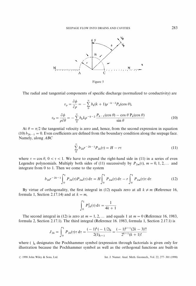
Figure 5

The radial and tangential components of specific discharge (normalized to conductivity) are

vo"L/

Lo"!

=+0

bk(k#1)o~k~2P

k(cos h ),

vh"L/oLh

"!

=+0

bkko~k~2

Pk~1

(cos h)!cos h Pk(cos h )

sin h(10)

At h"n/2 the tangential velocity is zero and, hence, from the second expression in equation(10) b

2k~1"0. Even coefficients are defined from the boundary condition along the seepage face.

Namely, along ABC

=+0

b2k

r~2k~1P2k

(q)"H!rq (11)

where q"cos h, 0(q(1. We have to expand the right-hand side in (11) in a series of evenLegendre polynomials. Multiply both sides of (11) successively by P

2m(q), m"0, 1, 2,2 and

integrate from 0 to 1. Then we come to the system

b2k

r~2k~1P1

0

P2k

(q)P2m

(q) dq"HP1

0

P2m

(q) dq!rP1

0

P2m

(q)q dq (12)

By virtue of orthogonality, the first integral in (12) equals zero at all kOm (Reference 16,formula 1, Section 2.17.14) and at k"m,

P1

0

P22k

(q) dq"1

4k#1

The second integral in (12) is zero at m"1, 2,2 and equals 1 at m"0 (Reference 16, 1983,formula 2, Section 2.17.1). The third integral (Reference 16. 1983, formula 1, Section 2.17.1) is

J2k"P

1

0

P2k

(q)q dq"(!1)k (!1/2)

k2(1)

k`1

"

(!1)k`1(2k!3)!!

2k`1(k#1)!

where ( )n

designates the Pochhammer symbol (expression through factorials is given only forillustration because the Pochhammer symbol as well as the orthogonal functions are built-in



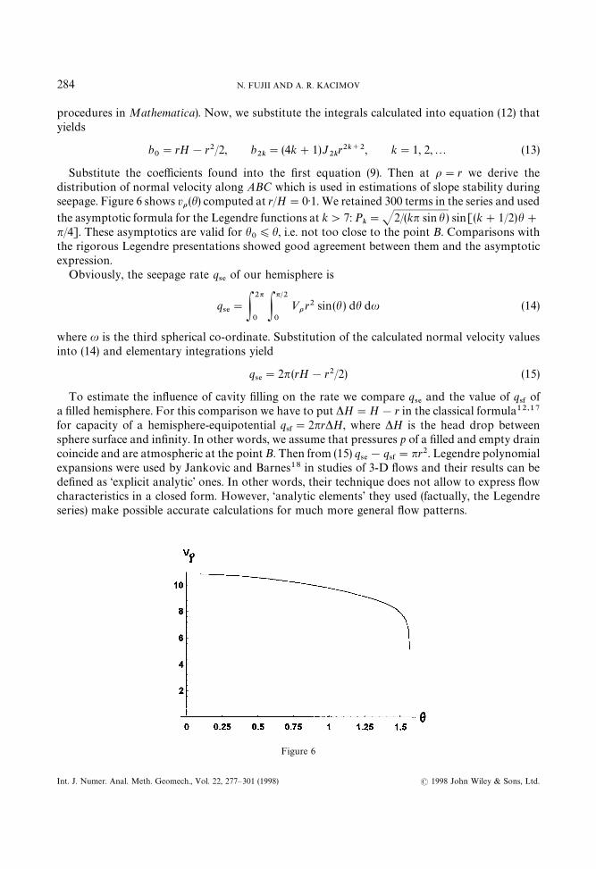
Figure 6

procedures in Mathematica). Now, we substitute the integrals calculated into equation (12) thatyields

b0"rH!r2/2, b

2k"(4k#1)J

2kr2k`2, k"1, 2,2 (13)

Substitute the coefficients found into the first equation (9). Then at o"r we derive thedistribution of normal velocity along ABC which is used in estimations of slope stability duringseepage. Figure 6 shows vo(h) computed at r/H"0)1. We retained 300 terms in the series and used

the asymptotic formula for the Legendre functions at k'7: Pk"J2/(kn sin h ) sin[(k#1/2)h#

n/4]. These asymptotics are valid for h0)h, i.e. not too close to the point B. Comparisons with

the rigorous Legendre presentations showed good agreement between them and the asymptoticexpression.

Obviously, the seepage rate q4%

of our hemisphere is

q4%"P

2n

0P

n@2

0

»or2 sin(h) dh du (14)

where u is the third spherical co-ordinate. Substitution of the calculated normal velocity valuesinto (14) and elementary integrations yield

q4%"2n(rH!r2/2) (15)

To estimate the influence of cavity filling on the rate we compare q4%

and the value of q4&

ofa filled hemisphere. For this comparison we have to put *H"H!r in the classical formula12,17for capacity of a hemisphere-equipotential q

4&"2nr*H, where *H is the head drop between

sphere surface and infinity. In other words, we assume that pressures p of a filled and empty draincoincide and are atmospheric at the point B. Then from (15) q

4%!q

4&"nr2. Legendre polynomial

expansions were used by Jankovic and Barnes18 in studies of 3-D flows and their results can bedefined as ‘explicit analytic’ ones. In other words, their technique does not allow to express flowcharacteristics in a closed form. However, ‘analytic elements’ they used (factually, the Legendreseries) make possible accurate calculations for much more general flow patterns.



Note, that a filled hemisphere in this flow pattern provides minimal seepage rate in the class ofarbitrary equipotential cavities of prescribed volume while the Weber disk was surmised toprovide minimal rate in the class of convex filled cavities of fixed surface area.17 As far as weknow, there are no analytic shape optimizations and corresponding rate estimations for 3-Dempty cavities.

It is worthy of mention, that solution for a Weber disk (which satisfies both the constant headand constant pressure conditions) under ponded surface was utilized for estimations of rate evenin a free surface flow19 that confirms usefulness of simple analytic formulae.

4. DRAINS IN HETEROGENEOUS AQUIFERS

Most soils are not homogeneous and seepage into horizontal drains in aquifers with various typesof heterogeneity was intensively studied analytically.1,4,20 In what follows, we illustrate how theknown solution for flow under a concrete dam can be converted to a scheme of seepage to slotdrains employing the Shulgasser21 formula. Then we compare the seepage rate into a semicirculardrain in a homogeneous aquifer (the Vedernikov formula) and in a two-layer aquifer (the formuladerived by the Polubarinova-Kochina method). We restrict ourselves with the case of filled drainsthough extension to empty ones is straightforward.

First, consider an aquifer composed of two layers of equal thickness ¹ but different conductivi-ties k

2and k

1(Figure 7(a)). Soil surface is ponded and a horizontal (AC) or vertical (DE) slot drain

(gallery) is placed on the impermeable bottom. The head drop between the soil surface and draincontour is H. The question is: how do the conductivity ratio s"k

1/k

2and the drain length

¸ influence the seepage rate?From the Schulgasser21 theorem the rate of the horizontal drain q

)is expressed through the

rate q$

of flow under an impervious dam (AC) in a porous massif with ‘inverted’ conductivityvalues depicted in Figure 7(b):

q)"k

1k2H2/q

$(16)

The rate of the vertical slot drain q7is derived through the value of rate q

4under an ‘equivalent’

sheet piling DE (Figure 7(b)) as

q7"k

1k2H2/q

4(17)

Solutions for the two flow patterns in Figure 7(b) were developed by Polubarinova-Kochina4(pp. 291—308). However, in the dam problem typical length ratios ¸/¹ are high and the graphs ofPolubarinova-Kochina do not fit the range usually encountered for drainage galleries. Hence, wehad to recalculate the values of flow rate. In particular, the value of q

$is

q$"

k1HJ

12 cos(ne)J

,

J"Pn@2

0

cos[2e arcsin(k sinx )] dx

J1!k2 sin2 x, J

1"P

n@2

0

cos[2e arcsin(k@ sin x )] dx

J1!k@2 sin2 x

e"1

narcsinS

1

1#s, k"tanh

n¸2¹

, k@"J1!k2 (18)



Figure 7

and the value of q4is

q4"

k1H tan(en)(J

3#J

4)

2J2

, at ¸'¹

"

k1H

J3#J

4C

k@2eJ5

cos(en )#0)5(J

3!J

4)tan(en )D , at ¸(¹ (19)

where

J2"J

3!J

4#J

5

2k@2esin(en)

, J3"P

n@2

0

(J1!k2 sin2 x#k cos x )2e dx

J1!k2 sin2 x

J4"P

n@2

0

(J1!k2 sin2 x!k cos x )2e dx

J1!k2 sin2 x, J

5"P

n@2

0

cos(2ex) dx

J1!k@2 sin2 x



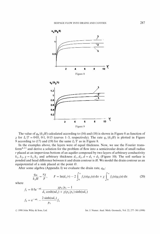
Figure 8

Figure 9

The value of q)/(k

2H) calculated according to (16) and (18) is shown in Figure 8 as function of

s for ¸/¹"0)05, 0)1, 0)15 (curves 1—3, respectively). The rate q7/(k

2H) is plotted in Figure

9 according to (17) and (19) for the same ¸/¹ as in Figure 8.In the examples above, the layers were of equal thickness. Now, we use the Fourier trans-

form4,11 and derive a solution for the problem of flow into a semicircular drain of small radiusr placed at an impervious bottom of an aquifer composed by two layers of arbitrary conductivityk1, k

2, s"k

1/k

2and arbitrary thickness d

1, d

2, d"d

1#d

2(Figure 10). The soil surface is

ponded and head difference between it and drain contour is H. We model the drain contour as anequipotential of a sink placed at the point O.

After some algebra (Appendix I) we evaluate the drain rate, q$3

:

q$3

k2H"

nsF

, F"ln(d1/r)!2 P

=

0

f1(a)g

1(a) da#s P

=

0

f2(a)g

2(a) da (20)

where

f1"0)5e~ad1

sp2/p

1!1

d1

cosh(ad1)#s(p

2/p

1) sinh(ad

1)

f2"e~ad1!

2 sinh(ad1)

p1

f1



Figure 10

p1"e~ad1#e~ad1~2ad2, p

2"e~ad1~2ad2

g1"

cosh(ad1)!cosh(ar)

a

g2"(1#e~2ad)

sinh(ad)!sinh(ad1)

a!(1!e~2ad)

cosh(ad)!cosh(ad1)

a(21)

At k2"k

1"k the Vedernikov5 formula for the rate q0

$3reads

q0$3"

nkH

arctanh(sin[n (1!r/d)/2])(22)

while the Polubarinova-Kochina4 (p. 355) approximate formula is q0$3"(nkH )/(ln[0)5nr/d]).

The rate q$3

/(k2H ) calculated according to (20) and (21) is plotted in Figure 11 as function of

s for r/H"0)05, d1/H"1, d

2/H"0)1, 1)0, 2)0 (curves 1—3, respectively). Mathematica allowed to

perform computations easily. In the limit s"1 our calculations fit the Vedernikov formula (22)well, while the Polubarinova-Kochina one leads to some discrepancy as was the case for a filleddrain in Section 2 above. Extension of the method to the case of three and more layers isstraightforward.

Note, that the Fourier transforms, Fourier series expansions (developed by Kirkham, see Baruaand Tiwari22 for recent references), conformal mappings and analytic continuation principles23allow to take into account rigorous conjugation conditions along division lines of different media.In combination with approximate analytic description4 of inhomogeneities it allows to comp-lement standard numerical codes.



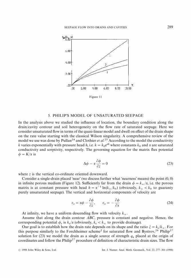
Figure 11

5. PHILIP’S MODEL OF UNSATURATED SEEPAGE

In the analysis above we studied the influence of location, the boundary condition along thedrain/cavity contour and soil heterogeneity on the flow rate of saturated seepage. Here weconsider unsaturated flow in terms of the quasi-linear model and dwell on effect of the drain shapeon the rate value starting with the classical Wilson singularity. A comprehensive review of themodel we use was done by Pullan24 and Clothier et al.25 According to the model the conductivityk varies exponentially with pressure head h, i.e. k"k

0eah where constants k

0and a are saturated

conductivity and sorptivity, respectively. The governing equation for the matrix flux potential/"K/a is

*/!aL/

Lz"0 (23)

where z is the vertical co-ordinate oriented downward.Consider a single-drain placed ‘near’ (we discuss further what ‘nearness’ means) the point (0, 0)

in infinite porous medium (Figure 12). Sufficiently far from the drain /"k=

/a, i.e. the porousmatrix is at constant pressure with head h"a~1 ln(k

=/k

0) (obviously, k

=(k

0to guaranty

purely unsaturated seepage). The vertical and horizontal components of velocity are

vz"a/!

L/

Lz, v

x"!

L/

Lx(24)

At infinity, we have a uniform descending flow with velocity k=

.Assume that along the drain contour ABC, pressure is constant and negative. Hence, the

corresponding potential /#is k

#/a (obviously, k

#(k

=to provide drainage).

Our goal is to establish how the drain rate depends on its shape and the ratio m"k#/k

=. For

this purpose similarly to the Forchheimer scheme2 for saturated flow and Bystrov,26 Philip27

solution for (23) we model the drain as a single source of strength q6

placed at the origin ofcoordinates and follow the Philip27 procedure of definition of characteristic drain sizes. The flow



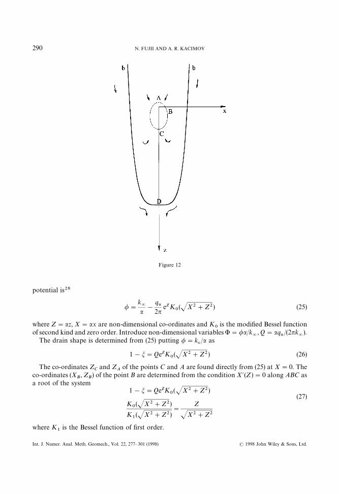
Figure 12

potential is28

/"

k=a!

q6

2neZK

0(JX2#Z2) (25)

where Z"az, X"ax are non-dimensional co-ordinates and K0

is the modified Bessel functionof second kind and zero order. Introduce non-dimensional variables '"/a/k

=, Q"aq

6/(2nk

=).

The drain shape is determined from (25) putting /"k#/a as

1!m"QeZK0(JX2#Z2) (26)

The co-ordinates ZC

and ZA

of the points C and A are found directly from (25) at X"0. Theco-ordinates (X

B, Z

B) of the point B are determined from the condition X@(Z)"0 along ABC as

a root of the system1!m"QeZK

0(JX2#Z2)

(27)K

0(JX2#Z2)

K1(JX2#Z2)

"

Z

JX2#Z2

where K1

is the Bessel function of first order.



Figure 13

Both (26) and (27) are solved using standard Mathematica routines.29 We define the horizontaland vertical sizes (recall that they are nondimensional) of the drain as b"X

Band

a"(ZC!Z

A)/2, correspondingly. We define position of the centre of the drain as

c"(ZC#Z

A)/2. Calculations show that ABC is an oval which can be approximated as an ellipse

and we determine the cross-sectional area of the drain as S"nab. The oval ratio we define ase"a/b and the value of f"c/z

Bcharacterizes deviation of the oval from an equivalent ellipse.

Figure 13 shows the values of e, f and k"Q/JS (curves 1—3, correspondingly) as functions ofg"1!m at Q"1. Note, that at sufficiently high values of /

#the corresponding drain ‘centre’ lies

far below the sink. It means the isobaric contour seeps mostly through its upper part.The drain captures a part of the descendant flow and the line b—b in Figure 12 is a separatrice

bisecting the flow. The stagnation point D can be found according to (23) from the conditionvz(0, z )"0 that in non-dimensional variables is reduced to

eZ[K1(Z)!K

0(Z )]"2/Q (28)

The root ZD

of (2) is shown in Figure 14 as function of Q. Note, that in 2-D saturated flow fora similar pattern of a single pumping well in uniform flow (Bear,30 pp. 323—324) the distancebetween the well and stagnation point is q/(2nv

=) where q is the well rate and v

=is the velocity of

the uniform flow. As we have mentioned, the case of an isobaric circle was studied by Lei9 thoughhe did not distinguish explicitly the separatrice and the drain catchment area.

Emphasize that all geometrical sizes of the drain evaluated are the same for the case of a cavitymodeled by a single source in infinite medium27 since potentials of the two flows differ only ina constant (/

=) though flow nets and velocity distributions clearly differ.

6. OPTIMAL SHAPE DESIGN

Since the classical studies of ancient Greeks, Saint-Venant, and Rayleygh shape optimization andcorresponding isoperimetric inequalities are investigated in many applications,17,31,32 in particu-lar, for seepage flows.33,34 The general statement is clear: what form of the boundary (or its part)



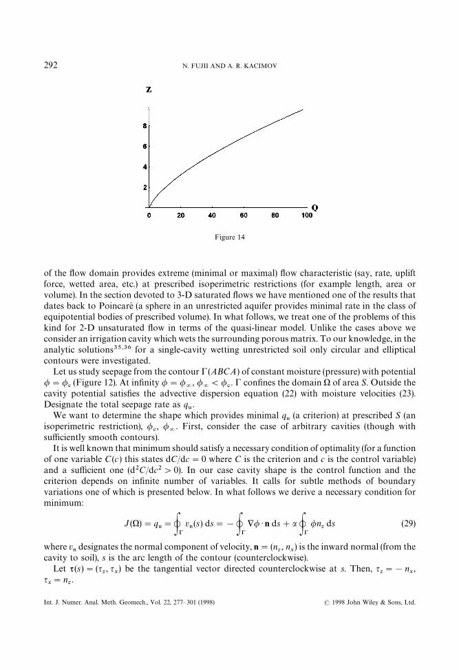
Figure 14

of the flow domain provides extreme (minimal or maximal) flow characteristic (say, rate, upliftforce, wetted area, etc.) at prescribed isoperimetric restrictions (for example length, area orvolume). In the section devoted to 3-D saturated flows we have mentioned one of the results thatdates back to Poincare (a sphere in an unrestricted aquifer provides minimal rate in the class ofequipotential bodies of prescribed volume). In what follows, we treat one of the problems of thiskind for 2-D unsaturated flow in terms of the quasi-linear model. Unlike the cases above weconsider an irrigation cavity which wets the surrounding porous matrix. To our knowledge, in theanalytic solutions35,36 for a single-cavity wetting unrestricted soil only circular and ellipticalcontours were investigated.

Let us study seepage from the contour ! (ABCA) of constant moisture (pressure) with potential/"/

#(Figure 12). At infinity /"/

=, /

=(/

#. ! confines the domain ) of area S. Outside the

cavity potential satisfies the advective dispersion equation (22) with moisture velocities (23).Designate the total seepage rate as q

6.

We want to determine the shape which provides minimal q6

(a criterion) at prescribed S (anisoperimetric restriction), /

#, /

=. First, consider the case of arbitrary cavities (though with

sufficiently smooth contours).It is well known that minimum should satisfy a necessary condition of optimality (for a function

of one variable C(c ) this states dC/dc"0 where C is the criterion and c is the control variable)and a sufficient one (d2C/dc2'0). In our case cavity shape is the control function and thecriterion depends on infinite number of variables. It calls for subtle methods of boundaryvariations one of which is presented below. In what follows we derive a necessary condition forminimum:

J ())"q6"Q! v

/(s) ds"!Q! +/ ) n ds#a Q! /n

zds (29)

where v/designates the normal component of velocity, n"(n

z, n

x) is the inward normal (from the

cavity to soil), s is the arc length of the contour (counterclockwise).Let s(s)"(q

z, q

x) be the tangential vector directed counterclockwise at s. Then, q

z"!n

x,

qx"n

z.



We can easily see that

dn

ds"

1

Rs (30)

hence, in turn

dsds

"A!dn

xds

,dn

zds B

"!

1

Rn (31)

where R denotes the radius of curvature at s. On ! the formula of integration by parts reads

Q! f @(s)g(s ) ds"Q! f (s)g@(s) ds (32)

Let us introduce a variation of !. Let o (s) be a smooth function of s. Let e be a number; itsabsolute value is small enough. We place segment eo(s) on the normal n at s such that positiveeo(s) lies on the normal n. If De D is small enough, the end points of the segments will form a closedcurve !e which and !

=enclose a new domain )e . When we consider the following boundary-

value problem:

*/e"aL/eLz

((z, x )3)e) (33)

/e"/#(const.) ((z, x )3!e) (34)

/e"/=

((z, x )3!=

) (35)

we can easily find that the first variation # of / defined by

/e!/"e##o (e) (36)

is the solution of

*#"aL#Lz

(in )) (37)

#"!

L/

Lno (on ! ) (38)

#"0 (at !=

) (39)

On the other hand, we see that the corresponding ne is given by

ne"n#(!eo@(s)s)#o(e ) (40)

through geometrical inspection. Similarly, we obtain

dse"A1#eoR#o(e)B ds (41)



Objective functional Je for /e is given by

Je"!Q!e

grad /e ) nedse#a Q!e

/enezdse (42)

The first term on the right-hand side of (42) is transformed as follows:

Q!e

grad /e )dse"Q!e

grad(/#e##o(e)) ) ne dse

"Q! grad / ) n ds

#e Q! G1

Rgrad / ) n#A

L2/

Lz2n2z#2

L2/

LzLxnznx#

L2/

Lx2n2xBH ds

#e Q!e

grad # ) n ds!e Q!e

o@(s)grad / ) s ds#o(e ) (43)

where we used (40) and (41).Introduce an adjoint variable p

!as the solution of the following boundary value problem:

*p!#a

Lp!

Lz"0 (in soil) (44)

p!"1 (at the cavity boundary) (45)

p!"0 (at infinity) (46)

Thanks to Green’s formula, we can calculate as follows:

P) (#*p!!p

!*#) da"Q!`!e

Ap!L#Ln

!#Lp

!Ln B ds

"Q! grad # ) n ds#Q!L/

Ln

Lp!

Lno ds (47)

where we used (38), (39), (45) and (46). Hence, using (37), (44), (38) and (39), we obtain

Q! grad # ) n ds#Q!L/Ln

Lp!

Lno ds"P) (#*p

!!p

!*#) da

"!P) AaLp

!Lz

##ap!

L#Lz B da

"!P) div(ap!# ) da

"Q! p!#a ) n ds#Q!=

p!#a ) n ds

"!Q! aL/

Lnon

zds (48)



where a"(a, 0).On the other hand, by integrating by parts, we obtain

!Q! o@(s)grad / ) s ds"Q! o(s )LLs

(grad /s ) ds

"Q! GALLs

grad /B ) s!1

Rgrad / ) nH o ds (49)

Substituting (48) and (49) into (43), we obtain

Q!e

grad /e ) dse"Q! grad / ) n ds#eQ! AL2/

Lz2n2z#2

L2/

LzLxnznx#

L2/

Lx2n2xB o ds

!e Q! AL/

Ln

Lp!

Lno#a

L/

LnnzoB ds

#e Q! ALLs

grad /B ) so#o (e) (50)

Similarly, we can see that

Q!e

/enezdse"Q! /n

zds#eQ! A

1

R/on

z#o

LLs

(/qz)B ds

"Q! /nzds#o (e) (51)

since (L//Ls) vanishes on !. From (50) we see that

Q!e

grad /e )dse!Q! grad / ) n ds"!e Q! AL/Ln

Lp!

Lno#a

L/Ln

nzoB ds

#e Q! AL2/

Lz2n2z#2

L2/

LzLxnznx#

L2/

Lx2n2xB o ds

#e Q! AL2/

Lz2n2z#!2

L2/

LzLxnznx#

L2/

Lx2n2xB o ds#o (e)

"!e Q! AL/Ln

Lp!

Lno#a

L/Ln

nzoB ds#ea Q!

L/Lz

o ds#o(e)

(52)Hence, if we define dJ by

Je!J"edJ#o (e) (53)

we observe that

dJ"!Q! AL/

Ln

Lp!

Ln#a

L/

Lnnz!a

L/

Lz B o ds (54)



Since admissible cavities must satisfy

P)c

da"S (55)

where S is the given area of cross-section of the cavities, we have

Q! o ds"0 (56)

If ) attains minimum q6, dJ must vanish for every o which satisfies (56). Thus, we obtain the

following necessary condition of minimum:If the cavity boundary ! attains a minimum q

6, then there exists a constant j (Lagrange

multiplier) such thatL/

Ln

Lp!

Ln#an

z

L/

Ln!a

LhLz

"j (57)

holds at every point on !.The known sink—source solutions of (23) and the solution of (44) are given by infinite series

expansions in terms of modified Bessel functions; it is difficult to test the condition (57) for thesesolutions. However, (54) gives the gradient of the objective function; (54) can be used fornumerical calculation of the optimal shape. As for more general and prototype shape optimiza-tion, the readers can refer Fujii.32

Preliminary computations based on the Concer35 solution and McLachlan37 asymptotics(small values of the ellipse aspect ratio) showed that starting with a circle and preservingcross-sectional area of a cavity we do can improve the criterion, i.e. minimize the rate (AppendixII). Nevertheless, matching of the rigorous necessary condition and the corresponding conditionfor an optimal ellipse (in some integral sense31) is still an unresolved problem.

7. CONCLUSION AND PERSPECTIVES

We addressed a number of problems for saturated and unsaturated, 2-D and 3-D flow patterns inhomogeneous and layered porous matrixes. Delving in the old books we found a number ofsolutions which seemed to be ponderous at the time they were developed. However, the progressin computer treatment of analytic expressions makes them competitive with standard numericalprocedures. In this way we applied the complex analysis, Fourier expansions and transform,optimal shape design methods and illustrated the simple and tractable solutions utilizingMathematica. Of most interest for us are optimization problems for seepage flows that can betreated analytically. Note, that by virtue of close analogy between the quasi-linear model forunsaturated seepage and advective dispersion model of neutral contaminant transport in subsur-face we plan to employ optimization methods in estimations of tracer distributions.

Obviously, the solutions are derived under severe simplifications about the flow and mediumand can serve as test, ‘back-of-an-envelope’ procedures in implementation of FDM-FEM codesto ‘real-world’ problems.

ACKNOWLEDGEMENTS

The second author thanks the Japanese Society for Promotion of Science (Grant RC 39226015)and Russian Foundation of Basic Research (Grant N96-0100844-96-01-00123) for financialsupport. Helpful comments of an anonymous reviewer are appreciated.



APPENDIX I

In what follows we describe in details derivations of the total rate for the flow in Figure 10(Section 4).

Factually, we use standard technique of Polubarinova-Kochina (Fourier integral presenta-tions). However, in the book of Olejnik (1979) which summarizes the problems solved by thismethod we could not find an analogous solution. Olejnik (and the authors he cites) have usedsome special tricks (series expansions) to derive the final formulae for total rate (it was necessaryin the pre-Mathematica years). We do not need any additional assumptions and performintegration without any simplifications.

Thus, we search for two analytic functions »1"u

1!iv

1"dw

1/dz and »

2"u

2!iv

2"

dw2/dz where w

1and w

2are complex potentials within the two layers, »

1and »

2are complex

conjugated velocities, u1,2

and v1,2

are horizontal and vertical components of the velocity. AlongMO we assume stream function t"0 and t"!q

$3along NO. Since the drain is filled we set

potential /"0 along its contour and /"!H along the flooded surface.Like in the vortex case treated by Polubarinova-Kochina (1977) we present »

1as

»1"!

q$3

nz#P

=

0

[A1(a)e*az#B

1(a)e~*az] da (58)

The first summand in equation (58) corresponds to the half-sink modelling our drain. Analog-ously, in the upper layer

»2"P

=

0

[A2(a)e*az#B

2(a)e~*az] da (59)

(the singular term is omitted because drain is located in the first layer).The complex coefficients A

1"a

r1#ia

i1, B

1"b

r1#ib

i1, A

2"a

r2#ia

i2, B

2"b

r2#ib

i2have to be found. To derive the eight unknown values we use the boundary conditions. Namely,along the horizontal bottom v

1"0. Hence, equating the imaginary part in (58) to zero we come

to ar1"b

r1and a

*1"!b

*1. Along the ponded surface u

2"0. Therefore, from (59) we derive

br2"!a

r2e~2ad and b

i2"!a

*2e~2ad.

Along the contact line of the layers two conditions hold. First, u1"su

2( jump in tangential

velocities). Present the singular term in (58) as

1/z"!i P=

0

e*az da

Equate the real part of (58) and real part of (59) multiplied by s. After elementary calculationswe come to

a*1

(ead1#e~ad1 )#q$3n

e~ad1"sa*2

(e~ad1#e~ad1~2ad2 )

ar1

(ead1#e~ad1 )"sar2

(e~ad1#e~ad1~2ad2)The second conjugation condition along the interface between two layers states that v

1"v

2(continuity of normal velocities). Therefore, equating imaginary parts of (58) and (59) along thisline we obtain

ar1

(e~ad1!ead1 )"ar2

(e~ad1#e~ad1~2ad2)q$3n

e~ad1#a*1

(e~ad1!ead1)"a*2

(e~ad1#e~ad1~2ad2 )



It follows immediately, that ar1"b

r1"a

r2"b

r2"0. Note, that this result could be obtained

from some simple symmetry reasons. However, we carried out all derivations to illustrate theprocedure. For a

*1and a

*2we have a system of linear equations which yields

a*1"

q$3

2ne~ad1

sp2/p

1!1

cosh(ad1)#sp

2/p

1sinh(ad

1)

(60)

a*2"

q$3

e~ad1np

1

!

2a*1

sinh(ad1)

p1

Thus, we derived completely our solution

»1"!

q$3

nz!2 P

=

0

a*1

sin(az) da

»2"i P

=

0

a*2

[cos(az )(1#e~2ad)#i sin(az ) (1!e~2ad )] da (61)

where a*1

and a*2

are defined by (60).However, to determine the total rate we have to circumvent a technical pitfall that is not

perfectly explained in textbooks (say, in the books by Oleynik and Polubarinova-Kochina).Namely, we perform integration of (61) and derive the complex potentials

w1"!

q$3n

ln z#2 P=

0

a*1

cos(az) da#w10

(62)

w2"i P

=

0

a*2 C

sin(az)

a(1#e~2ad)!

cos(az)

a(1!e~2ad)D da#w

20

Now, we employ the boundary conditions for / and t to find the constants of integration w10

,w20

. At the point z"ir the first complex potential w1"0. Hence, from the first equation (62)

w10"

q$3n

ln(ir)!2 P=

0

a*1

cos(air)

ada

In the first layer the potential at the point z"id1

is

/1"!

q$3n

ln(d1/r)#2 P

=

0

a*1

cosh(ad1)!cosh(ar)

ada (63)

At the point z"id the second complex potential is w2"!iq

$3/2!k

2H. Therefore, we can

determine w20

and the potential in the second layer is

/2"!k

2H#P

=

0

a*2 C

sinh(ad)

a(1#e~2ad)!

cosh(ad )

a(1!e~2ad)D da

#P=

0

a*2 C

!sinh(ad1)

a(1#e~2ad)!

cosh(ad1)

a(1!e~2ad)D da (64)

Now, continuity of the pressure (head) along the line y"id1yields /

1"s/

2which we apply at

the point z"id1. In other words, we write a linear combination of (63) and (64) with s as

a coefficient. It allows to get the expression q$3/H"f (k

2, d

1, d

2, r, s ), i.e. formula (19).



APPENDIX II

Consider seepage from elliptical cavities wetting surrounding dry soil. We show how theConcer35 solution can be implemented for optimization in the class of ellipses which allow tofollow the main trend in rate value under shape variations. Note, that considering narrowerclasses of curves is standard to approach the optimum. In this case the objective can be oftenapproximated with good accuracy.38 Thus, let the feeding contour ABCA in Figure 12 is an

ellipse with axes a, b, focus distance c"Ja2!b2, cross-sectional area S"nab and rate q%.

Hence, in the class of ellipses under study the optimization problem is reduced to search for theaxis ratio b/a providing minimum q

eat fixed S.

First, note that the Philip36 solution coincides (up to notations) with the Concer35 solution. Inparticular, Philip’s formula (38) for non-dimensional total rate from a cylindrical cavity beingmultiplied by 2nr, where r is the cylinder radius, brings just the same result as formula (27) ofConcer.35

The value of q%for an elliptical cavity we calculate after slight modification of the Concer (1959)

solution:

qe"un sinh s

0

=+n/0

EnFek

n(s0, !g)[(!1)n

=+r/0

(!1)rA2n2r

(I2r`1

(u cosh s0)#I

2r~1(u cosh(s

0))

#(!1)n=+r/0

(!1)rB2n`12r`1

(I2r`2

(u cosh s0)#I

2r(u cosh(s

0))]

#2n=+n/0

EnFek@

n(s0, !g )[(!1)n

=+r/0

(!1)r A2n2r

I2r

(u cosh s0)

#(!1)n=+r/0

(!1)rB2n`12r`1

I2r`1

(u cosh s0)] (65)

where s0"arctanh(b/a), g"(ac/4)2, u"Jg/2. Note that our g is q of Concer. Coefficients E

nin

(65) are found from the boundary condition along the cavity contour as

En"

/#bn

Fekn(s0, !g )

,

bn"

:2n0

cen(t, !g)e~a cost dt

:2n0

ce2n(t, !g ) dt

Definitions of the Mathieu Fek, ce and Bessel I functions are from McLachlan.37 Note, that weassume coefficient normalization according to Section 2.11 of McLachlan.

We considered ellipses with nearly equal axes (gP0). In this case we used the asymptoticrepresentations for coefficient from Section 3.33 of McLachlan. We calculated series expansionsof Fek functions from Section 8.30 of McLachlan. We also used series expansions for ce

0, ce

1, ce

2,

se1, se

2and their derivatives form Sections 2)13, 2)14, 2)150 of McLachlan. Same expansions we

used to calculate integrals in formulae for b/. Computations showed decrease in q

%at fixed S with

increase of a/b. However, the following questions are still open. First, it is unclear, whetherimprove of the criterion can be tracked further in a/b using asymptotics of small g. Intuitively it is



not clear, how prolonged will be the optimal ellipse. Nevertheless, we surmise existence ofa unique global optimum in the class of elliptic curves, i.e. a unique a/b value providing theminimum of q

%. This guess is based on our experience of optimization in the case of saturated

flows. Factually, existence of a nontrivial minimum can be explained just as in minimization ofthe rate in Section 2: very prolate and very oblate cavities of constant area (‘needles’ placed alongor perpendicular to the vertical axes) give infinitely high rates. Hence, an ‘intermediate’ ellipse hasto provide minimum (though uniquiness of the extremum is not obvious and counter-intuitiveexamples were obtained just in the class of ellipses39). Second, it may be better to use not theasymptotics but implement the general procedure for determination of coefficients37 or build-inprocedures for Mathieu functions from 3.0 version of Mathematica.

However, analysis of the Concer solution was instructive in the following sense. Namely,instead of attempts to satisfy the constant pressure conditions along a prescribed contour (as inthe Concer and Philip solutions) it seems to be interesting to meet the necessary condition ofoptimality from our Section 6 using the approach from Section 5. Namely, the first term inConcer’s expansion (11) is just a point source solution (Wilson’s singularity). Let us retain thesecond term K

1(r) cos(h). Then we can operate with the coefficient E

1and try to minimize the

rate from the corresponding cavity (this rate is easily determined from E0and E

1). The contour of

this E0!E

1cavity we can define according to the condition /"/

#. In other words, fixing the

cross-sectional area we have to solve an equation similar to (26) from Section 5 of our paper. Theprocedure can be extended further for E

2, E

3, etc. This approach was employed for optimization

in the case of the Poisson equation.40

REFERENCES

1. Drainage of Agricultural ¸ands, Ed. J. N. Luthin, ASA, Madison, 1957.2. P. Forchheimer, Hydraulik, Teubner Verlag, Wien, 1930.3. R. A. Freeze and J. A. Cherry, Groundwater, Prentice-Hall, Englewood Cliffs, NJ, 1979.4. P. Ya. Polubarinova-Kochina, ¹heory of Ground ¼ater Movement, Nauka, Moscow, 1977 (in Russian).5. V. V. Vedernikov, ¹heory of Filtration in Soils and Its Application in Problems of Irrigation and Drainage, Gosstrojiz-

dat, Moscow, 1939 (in Russian).6. S. Khan and K. R. Rushton, ‘Reapraisal of flow to tile drains. I. Steady state response’, J. Hydrol. 183, 351—366

(1996).7. R. E. Goodman, D. G. Moye, A. van Schalkwyk and I. Javandel, ‘Ground water inflows during tunnel driving’, Engng.

Geol. 2, 39—56 (1965).8. D. Ford and P. Williams, Karst Geomorphology and Hydrology, Unwin, London, 1989.9. S. Lei, ‘An analytical solution for steady flow into a tunnel’, Proc. Conf. Analytic-based Modeling of Groundwater Flow,

Vol. 2, Netherlands Inst. of Applied Geoscience, TNO, 1997, pp. 447—454.10. N. B. Ilyinsky and A. R. Kacimov, Problems of seepage to empty ditch and drain’, ¼ater Resour. Res., 28, 871—876

(1992).11. M. Muskat, Physical Principles of Oil Production, McGraw-Hill, New York, 1946.12. H. Ebert, Physikalisches ¹aschenbuch, Fiedr. Vieweg & Sohn, Braunschweig, 1957.13. S. Kutateladse, Handbook on Heat ¹ransfer and Hydrodynamic Resistance, Energoatomizdat, Moscow, 1990 (in

Russian).14. J. Crank, ¹he Mathematics of Diffusion, Clarendon Press, Oxford, 1975.15. A. R. Kacimov, ‘Explicit solutions for seepage infiltrating into a porous earth dam due to precipitation’, Int. J. Numer.

Anal. Meth. Geomech. 20, 715—723 (1996).16. A. P. Prudnikov, Yu.A. Brychkov and O. I. Marichev, Integrals and Series. Special Functions, Nauka, Moscow, 1983

(in Russian).17. G. Polya and G. Szego, Isoperimetric Inequalities in Mathematical Physics, Princeton University Press, Princeton,

1951.18. I. Jankovic and R. Barnes, ‘Three-dimensional flow through large numbers of spheroidal inhomogeneities’, Proc.

Conf. Analytic-based Modeling of Groundwater Flow, Vol. 2 Netherlands Inst. of Applied Geoscience, TNO, 1997,425—433.



19. E. G. Youngs, G. Spoor and G. R. Goodall, ‘Infiltration from surface ponds into soils overlying a very permeablesubstratum’, J. Hydrol. 186, 327—334 (1996).

20. A. Ya. Olejnik, Geohydrodynamics of Drainage, Naukova Dumka, Kiev, 1979 (in Russian).21. K. Schulgasser, ‘A reciprocal theorem in two-dimensional heat transfer and its implications’, Int. Commun. Heat Mass

¹ransfer, 19, 639—649 (1992).22. G. Barua and K. N. Tiwari, ‘Theories of ditch drainage in layered anisotropic soil’, J. Irrigation Drain. Engng., 122 (6),

321—330 (1996).23. A. R. Kacimov and Yu.V. Obnosov, ‘Explicit solution to a problem of seepage in a checker-board massif ’, ¹ransport

in Porous Media, 28 (1), 109—124 (1997).24. A. Pullan, ‘The quasilinear approximation for unsaturated porous media flow’, ¼ater Resour. Res., 26, 1219—1234

(1990).25. B. E. Clothier, S. R. Green and H. Katou, ‘Multidimensional infiltration: points, furrows, basins, wells and disks’, Soil

Sci. Soc. Amer. J., 59, 286—292 (1995).26. K. N. Bystrov, ‘Determination of flows with point singularities in bended layers of varying density’, Izv. AN SSSR,

Mekh. Zhidk. Gasa (Fluid Dynamics), 3 (1), 169—175 (1968).27. J. R. Philip, ‘Theory of infiltration’, Adv. Hydrosci., 5, 215—296 (1969).28. A. W. Warrick and G. G. Fennemore, ‘Unsaturated water flow around obstructions simulated by two-dimensional

Rankine bodies’, Adv. ¼ater Resour., 18 (6), 375—382 (1995).29. T. B. Bahder, Mathematica for Scientists and Engineers, Addison-Wesley, Reading, MA, 1995.30. J. Bear, Dynamics of Fluids in Porous Media, Elsevier, New York, 1972.31. O. Pironneau, Optimal Shape Design for Elliptic Systems, Springer, New York, 1984.32. N. Fujii, ‘Second-order necessary conditions in a domain optimization problem’, J. Optim. ¹heory Appl. 65 (2),

223—244 (1990).33. J. R. Philip, J. H. Knight and R. T. Waechter, ‘The seepage exclusion problem for a parabolic and paraboloidal

cavities’, ¼ater Resour. Res., 25, 605—618 (1989).34. N. B. Ilyinsky and A. R. Kacimov, ‘The estimation of integral seepage characteristics of hydraulic structures in terms

of the theory of inverse boundary-value problems’, Zeitschr. Angew. Math. Mech., 72, 103—112 (1992).35. D. B. Concer, ‘Heat flow towards a moving cavity’, Quart. J. Mech. Appl. Math., 12, Pt. 2, 222—232 (1959).36. J. R. Philip, ‘Steady infiltration from circular cylindrical cavities’, Soil Sci. Soc. Am. J., 48, 270—278 (1984).37. N. W. McLachlan, ¹heory and Application of Mathieu Functions, Clarendon Press, Oxford, 1947.38. A. R. Kacimov, ‘Seepage optimization for a trapezoidal channel’, J. Irrigation Drainage, ASCE, 118, 520—526 (1992).39. A. R. Kacimov and Yu.V. Obnosov, ‘Explicit, rigorous solutions to 2-D heat transfer: Two-component media and

optimization of cooling fins’, Int. J. Heat Mass ¹ransfer, 40, 1191—1196 (1997).40. S. Belov and N. Fujii, ‘Symmetry and sufficient conditions of optimality in a domain optimization problem’, Control

Cybernet. 26 (1), 45—56 (1997).



Documents

Analytically computed rates of seepage flow into drains and cavities