This content has been downloaded from IOPscience. Please scroll down to see the full text.

Download details:

IP Address: 201.172.110.154

This content was downloaded on 26/06/2016 at 08:18

Please note that terms and conditions apply.

Analytical study of the magnetic field generated by multipolar magnetic configuration

View the table of contents for this issue, or go to the journal homepage for more

2016 J. Phys.: Conf. Ser. 687 012023

(http://iopscience.iop.org/1742-6596/687/1/012023)

Home Search Collections Journals About Contact us My IOPscience

Analytical study of the magnetic field generated by

multipolar magnetic configuration

M T Murillo Acevedo1,2, V D Dugar-Zhabon2 and O Otero2

1 Universidad Santo Tomas, Bucaramanga, Colombia.2 Universidad Industrial de Santander, Bucaramanga, Colombia.

E-mail: oswaldoterolarte@gmail.com

Abstract. The magneto-statics field from a parallelepiped magnet which can turn around an axis, is the first step to find the whole magnetic field in a multipolar configuration. This configuration is present in the ion sources, which are heated by electron cyclotron resonance. We present the analytic formulas to calculate this magnetic field outside the volume of the magnet. To model the magnet, we considered a constant magnetization vector inside of magnet volume. Therefore, the magnetic scalar potential method can be used. We present the results by a hexapolar system. Their magnetic field components are calculated on confinement region, several graphics are shown with directions and magnitude’s gradients of the magnetic field to help understand better the confinement system. Our results are confronted with experimental ones. These formulas are very useful in research of plasma magnetic confinement in ion sources through computational simulations.

1. IntroductionTo confine plasma in an electron cyclotron resonance (ECR) ion source, a transversal multicuspmagnetic field is used. This field helps to remove magnetohydrodynamics instabilities due to theconvex curvature of mirror’s magnetic field [1]. It is common to use six or eight parallelepipedmagnets around cylinder discharge camera to create a cusp geometric form of magnetic field,which changes the magnetic field curvature. The analytic calculation of magnetic field isuseful in plasma dynamics computational simulations. Although several models use multi-polar approximation, the interaction between the magneto-statics field of the trap and themicrowaves field exerts the biggest influence over plasma behaviour; therefore is very importantto get a better model to calculate magnetic field. An analytical result was published in [4] for themodelling of parallelepipedic magnets of various polarisation directions. However, we presentthe case, when the polarisation vector stays constant, but the whole magnet can turn aroundan axis and we solve each indetermination present in the formulas. Therefore, our formulasare more useful for calculate multipolar magnetic field. The multipolar magnetic field has beenimportant in plasma studying from microelectronics fabrication to the fabrication flat paneldisplay device [2]. This system of magnetic field is used in some configurations of magneticconfinement [3]. It starts from a magnetic scalar potential [5], but its equations are not solved,instead the magnetic fields components are calculated by using gradients, transforming thoseequations until they transform into a integrable form. The final equations are using to calculatethe magnetic field into a cubic mesh. The magnet is considered as a material with constantmagnetisation vector inside it, and zero outside. The equations are solved only in confinement

IMRMPT2015 IOP PublishingJournal of Physics: Conference Series 687 (2016) 012023 doi:10.1088/1742-6596/687/1/012023

Content from this work may be used under the terms of the Creative Commons Attribution 3.0 licence. Any further distributionof this work must maintain attribution to the author(s) and the title of the work, journal citation and DOI.

Published under licence by IOP Publishing Ltd 1

volume, which is found outside magnets inner region. Several pictures show the curvature andmagnitudes gradients.

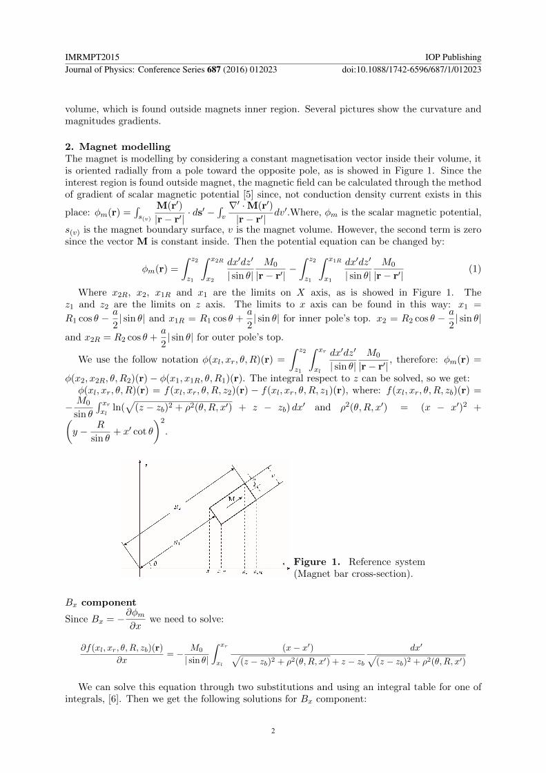
2. Magnet modellingThe magnet is modelling by considering a constant magnetisation vector inside their volume, itis oriented radially from a pole toward the opposite pole, as is showed in Figure 1. Since theinterest region is found outside magnet, the magnetic field can be calculated through the methodof gradient of scalar magnetic potential [5] since, not conduction density current exists in this

place: φm(r) =∫s(v)

M(r′)

|r− r′|· ds′ −

∫v

∇′ ·M(r′)

|r− r′|dv′.Where, φm is the scalar magnetic potential,

s(v) is the magnet boundary surface, v is the magnet volume. However, the second term is zerosince the vector M is constant inside. Then the potential equation can be changed by:

φm(r) =

∫ z2

z1

∫ x2R

x2

dx′dz′

| sin θ|M0

|r− r′|−∫ z2

z1

∫ x1R

x1

dx′dz′

| sin θ|M0

|r− r′|(1)

Where x2R, x2, x1R and x1 are the limits on X axis, as is showed in Figure 1. Thez1 and z2 are the limits on z axis. The limits to x axis can be found in this way: x1 =

R1 cos θ − a

2| sin θ| and x1R = R1 cos θ +

a

2| sin θ| for inner pole’s top. x2 = R2 cos θ − a

2| sin θ|

and x2R = R2 cos θ +a

2| sin θ| for outer pole’s top.

We use the follow notation φ(xl, xr, θ, R)(r) =

∫ z2

z1

∫ xr

xl

dx′dz′

| sin θ|M0

|r− r′|, therefore: φm(r) =

φ(x2, x2R, θ, R2)(r)− φ(x1, x1R, θ, R1)(r). The integral respect to z can be solved, so we get:φ(xl, xr, θ, R)(r) = f(xl, xr, θ, R, z2)(r) − f(xl, xr, θ, R, z1)(r), where: f(xl, xr, θ, R, zb)(r) =

− M0

sin θ

∫ xrxl

ln(√

(z − zb)2 + ρ2(θ,R, x′) + z − zb) dx′ and ρ2(θ,R, x′) = (x − x′)2 +(

y − R

sin θ+ x′ cot θ

)2

.

Figure 1. Reference system(Magnet bar cross-section).

Bx component

Since Bx = −∂φm∂x

we need to solve:

∂f(xl, xr, θ, R, zb)(r)

∂x= − M0

| sin θ|

∫ xr

xl

(x− x′)√(z − zb)2 + ρ2(θ,R, x′) + z − zb

dx′√(z − zb)2 + ρ2(θ,R, x′)

We can solve this equation through two substitutions and using an integral table for one ofintegrals, [6]. Then we get the following solutions for Bx component:

IMRMPT2015 IOP PublishingJournal of Physics: Conference Series 687 (2016) 012023 doi:10.1088/1742-6596/687/1/012023

2

Bx =− p(R2, θ)[S(θ,R2, z2, x2R)(r)− S(θ,R2, z2, x2)(r)− S(θ,R2, z1, x2R)(r) + S(θ,R2, z1, x2)(r)

]+ p(R1, θ)

[S(θ,R1, z2, x1R)(r)− S(θ,R1, z2, x1)(r)− S(θ,R1, z1, x1R)(r) + S(θ,R1, z1, x1)(r)

]+ | sin θ|

[D(x2R, θ, R2, z1, z2) +D(x2, θ, R2, z2, z1) +D(x1R, θ, R1, z2, z1) +D(x1, θ, R1, z1, z2)

]Where:

p(R, θ) =

| sin θ|(x+ cos θ(y sin θ −R)− x sin2 θ)√

x2 sin2 θ + (y sin θ −R)2 − (cos θ(y sin θ −R)− x sin2 θ)2If y sin θ −R 6= 0,

| cos θ| If y sin θ −R = 0

S(θ,R, zb, x′)(r) = −2M0 arctan

(u(θ,R, x ′) +

√q2(θ,R, zb) + u2(θ,R, x ′) + (z − zb)| sin θ|

l(θ,R)

)

D(xb, θ, R, zr, zl) =

M0 ln

(z − zlz − zr

)If sin2 θ = 1 ∧ y sin θ −R = 0 ∧ xb − x = 0,

M0 ln

(Dt(xb, θ, R, zr)

Dt(xb, θ, R, zl)

)Elsewhere

Dt(xb, θ, R, zb) =√q2(θ,R, zb) + u2(θ,R, xb) + (z − zb)| sin θ|

u(θ,R, x ′) = x ′ + cos θ(y sin θ −R)− x sin2 θ

h2(θ,R) = x2 +

(y − R

sin θ

)2

−(

cos θ

(y − R

sin θ

)− x sin θ

)2

Then:

q2(θ,R, zb) =[(z − zb)2 + x2

]sin2 θ + (y sin θ −R)2 −

[cos θ(y sin θ −R)− x sin2 θ

]2l(θ,R) = | sin θ|h(θ,R) =

√x2 sin2 θ + (y sin θ −R)2 −

[cos θ(y sin θ −R)− x sin2 θ

]2

By componentFor By component, we have:

By = j(R2, θ)[−S(θ,R2, z2, x2R)(r) + S(θ,R2, z2, x2)(r) + S(θ,R2, z1, x2R)(r)− S(θ,R2, z1, x2)(r)

]+

j(R1, θ)[S(θ,R1, z2, x1R)(r)− S(θ,R1, z2, x1)(r)− S(θ,R1, z1, x1R)(r) + S(θ,R1, z1, x1)(r)

]+

| sin θ|sin θ

cos θ[D(x1, θ, R1, z2, z1) +D(x1R, θ, R1, z1, z2) +D(x2R, θ, R2, z2, z1) +D(x2, θ, R2, z1, z2)

]Where:

j(R, θ) =

y| sin θ| −R | sin θ|

sin θ+(x sin2 θ − cos θ(y sin θ −R)

)cos θ

| sin θ|sin θ√

x2 sin2 θ + (y sin θ −R)2 − (cos θ(y sin θ −R)− x sin2 θ)2If y sin θ −R 6= 0,

sin θ cos θ

| cos θ|Otherwise

IMRMPT2015 IOP PublishingJournal of Physics: Conference Series 687 (2016) 012023 doi:10.1088/1742-6596/687/1/012023

3

Bz componentFor Bz component, the integral is more simple; first we integrate respect to x′ variable doingthe previous substitutions and then integrate with z′:

Bz = M0 ln

(k(θ,R2, z2, xR2)k(θ,R2, z1, x2)k(θ,R1, z1, xR1)k(θ,R1, z2, x1)

k(θ,R2, z1, xR2)k(θ,R2, z2, x2)k(θ,R1, z2, xR1)k(θ,R1, z1, x1)

)Where, k(θ,R, zb, xb) =

√q2(θ,R, zb) + u2(θ,R, x′) + u(θ,R, x′).

Results for θ = 0 or θ = 180◦

Since these formulas do not work when θ = 0 or θ = 180◦, because in this cases we have:|r− r′| =

√(z − z′)2 + (x−R cos θ)2 + (y − y′)2.

We use the follow notation, φ0(yl, yr, θ, R)(r) =

∫ z2

z1

∫ yr

yl

M0 dy′dz′√

(z − z′)2 + (x−R cos θ)2 + (y − y′)2.

therefore, we have:

φ0(yl, yr, θ, R)(r) = f0(yl, yr, θ, R, z2)(r)− f0(yl, yr, θ, R, z1)(r)

Where:

f0(yl, yr, θ, R, zb)(r) = −M0

∫ yr

yl

ln

(√(z − zb)2 + ρ20(θ,R, y

′) + z − zb)dy′

Bx0 component (with θ = 0)

Bx0 = − S0

(θ,R2, z2,

a

2

)(r) + S0

(θ,R2, z2,−

a

2

)(r) + S0

(θ,R2, z1,

a

2

)(r) − S0

(θ,R2, z1,−

a

2

)(r)

+ S0

(θ,R1, z2,

a

2

)(r) − S0

(θ,R1, z2,−

a

2

)(r) − S0

(θ,R1, z1,

a

2

)(r) + S0

(θ,R1, z1,−

a

2

)(r)

Where:

S0(θ,R, zb, yb)(r) =

0 If x−R cos θ = 0,

2M0x−R cos θ

|x−R cos θ|arctan

y − yb +√q20(θ,R, zb) + (y − yb)2 + (z − zb)

|x−R cos θ|

Otherwise

q20(θ,R, zb) = (z − zb)2 + (x−R cos θ)2

By0 component (with θ = 0)

By0 = D0

(θ,R2,

a

2, z1, z2

)(r) +D0

(θ,R2,−

a

2, z2, z1

)(r) +D0

(θ,R1,

a

2, z2, z1

)(r)

+D0

(θ,R1,−

a

2, z1, z2

)(r)

Where:

D0(θ,R, yb, zn, zd)(r) =

M0 ln

(|z − zd||z − zn|

)If x−R cos θ = 0 ∧ y − yb = 0,

M0 ln

(Dt0(θ,R, yb, zn)

Dt0(θ,R, yb, zd)

)otherwise

IMRMPT2015 IOP PublishingJournal of Physics: Conference Series 687 (2016) 012023 doi:10.1088/1742-6596/687/1/012023

4

Bz0 component (with θ = 0)

Bz0 = M0 ln

k0(θ,R2,−

a

2, z2

)k0

(θ,R2,

a

2, z1

)k0

(θ,R1,

a

2, z2

)k0

(θ,R1,−

a

2, z1

)k0

(θ,R2,

a

2, z2

)k0

(θ,R2,−

a

2, z1

)k0

(θ,R1,−

a

2, z2

)k0

(θ,R1,

a

2, z1

)

Where:

k0(θ,R, yb, zb) =√q20(θ,R, zb) + (y − yb)2 + y − yb

We present a picture of magnetic field from a cubic magnet of 4 cm length, with amagnetization vector of 518.67G of magnitude (see Figure 2). To confront this results, wetake data from Dexter Magnetic Tecnologies [7]. We take a cubic magnet with θ = 270◦,R1 = 0 in, R2 = 2 in, z1 = −1 in, z2 = 1 in, and a = 2 in; Residual induction (Br) G= 500,Material type, Nd -Fe -B. We use a point (xp, yp, zp) to calibrate the magnetic field magnitude, forexample we take M0 = 1 and calculate the magnetic field magnitude in this point, through ourformulas, called Bf (xp, yp, zp). Then we get the experimental result called Be(xp, yp, zp), thenM0 = Be(xp, yp, zp)/Bf (xp, yp, zp), this way we can get the correct magnetization vector, in thiscase is −37.894G. We put both experimental and simulated results in a Table 1. Therefore theseresults help us to show the validity of our formulas. Now we present the results for a hexapolesystem.

Table 1. Confront of data.Coordinates (in) B (G) Experimental B (G) Simulated

x y z Bx By Bz Bx By Bz

0 1 0 0 64.182 0 0 64.18203 00 2 0 0 21.6 0 0 21.59964 00 3 0 0 9.352 0 0 9.35169 00 4 0 0 4.824 0 0 4.82424 00 10 0 0 0.455 0 0 0.45542 00 1 1 0 38.530 29.885 0 38.53027 29.885340 1 2 0 6.546 20.439 0 6.54579 20.439200 1 3 0 -0.621 8.948 0 -0.62051 8.948040 0 3 0 -6.803 8.258 0 -6.80321 8.257550 -1 2 0 -32.091 0 0 -32.09102 01 1 1 20.59 23.287 20.59 20.59032 23.28694 20.590322 1 1 15.491 3.856 7.452 15.49089 3.85553 7.45216

Table 2. Physical scheme(hexapolar system).

3. Hexapolar systemThe physical system consists in a six parallelepiped bar magnets placed on the outside of acylinder, in alternating North/South polarizations, whose poles are targeted radially; this systemis showed in Figure 2.

The cylinder chamber radius is 3.9956cm, with length of 25.9720cm. Longitudinal size magnetbar is 21.0cm, the inner pole radius is R1 = 4.1cm in Figure 2; the external pole radius isR2 = 7.1cm, width a = 2.5cm. For hexapole field simulation we take the following anglesθ = 30◦, 90◦, 150◦, 210◦, 270◦ and 330◦. The field graphic on XY section (plane z = 0cm) isshowed in Figure 3; where the cusp curvature is seen near to magnetic pole zone. In this figurewe can see a gradient radial from the colour scale of field magnitude toward Z axis; this propertyis necessary to press the plasma back inside camera discharge.

The field on z = 10.0cm plane (See Figure 4) is like one central configuration since it isinside region covered by hexapole system. The field on z = 12.5cm plane (Figure 5) is morelongitudinal, specially in regions near magnet poles; since this zone is outside of hexapole region.The longitudinal field view on x = 0cm plane, is given in Figure 6, the magnetic field becomesmore longitudinal, outside of region covered by magnets, in the zone near to the magnets.

IMRMPT2015 IOP PublishingJournal of Physics: Conference Series 687 (2016) 012023 doi:10.1088/1742-6596/687/1/012023

5

Figure 2. Physical system.

Figure 3. XY view (planez = 0.0cm) of the magneticfield.

Figure 4. XY view (planez = 10.0cm) of the magneticfield.

Figure 5. XY view(plane z = 12.5cm) of themagnetic field.

Figure 6. YZ view (plane x = 0.0cm) of themagnetic field.

4. ConclusionThe analytic calculation from a parallelepiped magnet, which can turn around an axis is veryimportant to researchers on plasma physics under multipolar magnetic field, for example, inplasma magnetic confinement in ECR sources, since hexapole magnetic field configurations arean important term to improve the plasma dynamics simulations. Using an approximate value ofmagnetic field can cause mistakes. Although these errors can be small, the plasma simulationscycles need to be performed many times to reach the stability of the system. Therefore theerrors can increase when the number cycles grow. These calculations serve to help reducecomputational effects over the plasma behaviour simulated.

References[1] A Dinklage T Klinger G Marx and L Schweikhard 2005 Plasma physics confinement, transport and collective

effects 1st ed (Berlin: Springer-Verlag) p 148[2] K Kim, Y Lee, S Kyong and G Yeom 2004 Surface and Coatings Technology 177-178 752[3] H Takekida and K Nanbu 2004 Phys D Appl Phys 37 1800[4] R Ravaud and G Lemarquand 2009 Progress in Electromagnetics Research 98 207[5] J Jackson 1999 Classical Electrodynamics 3rd ed (United States of America: John Wiley & Sons Inc) pp

195-197[6] H Bristol 1957 Tables of integrals and other mathematical data 3rd ed (New York: The macmillan company)

p 93[7] Dexter Magnetic Tecnologies 2015 Field calculations for a rectangle (http://www.dextermag.com/resource-

center/magnetic-field-calculators/field-calculations-for-rectangle)

IMRMPT2015 IOP PublishingJournal of Physics: Conference Series 687 (2016) 012023 doi:10.1088/1742-6596/687/1/012023

6