Analytical solutions for solute transport insaturated porous media with semi-infinite or

finite thickness

Youn Sim & Constantinos V. Chrysikopoulos*Department of Civil and Environmental Engineering, University of California, Irvine, CA 92697, USA

(Received 5 April 1997; revised 19 June 1998; accepted 25 June 1998)

Three-dimensional analytical solutions for solute transport in saturated, homogeneousporous media are developed. The models account for three-dimensional dispersion ina uniform flow field, first-order decay of aqueous phase and sorbed solutes withdifferent decay rates, and nonequilibrium solute sorption onto the solid matrix of theporous formation. The governing solute transport equations are solved analytically byemploying Laplace, Fourier and finite Fourier cosine transform techniques. Porousmedia with either semi-infinite or finite thickness are considered. Furthermore,continuous as well as periodic source loadings from either a point or an elliptic sourcegeometry are examined. The effect of aquifer boundary conditions as well as thesource geometry on solute transport in subsurface porous formations is investigated.q 1999 Elsevier Science Ltd. All rights reserved.

Keywords:solute transport, analytical solution, multidimensional systems, nonequili-brium sorption, first-order decay.

NOMENCLATUREa semi-axis of the elliptic source parallel to thex-

axis [L]

a1, a2 defined in eqns (22) and (23), respectively

A defined in eqn (5)

b semi-axis of the elliptic source parallel to they-axis [L]

B defined in eqn (6)

C solute concentration in suspension (liquidphase) [M L¹3]

C0 source concentration [M L¹3]

C* sorbed solute concentration (solute mass/solidsmass) [M M¹1]

C` steady-state solute concentration in the absenceof decay [M L¹3]

Dx longitudinal hydrodynamic dispersion coeffi-cient [L2 t¹1]

Dy lateral hydrodynamic dispersion coefficient [L2 t¹1]

Dz vertical hydrodynamic dispersion coefficient[L 2 t¹1]

erf[x] error function, equal to(2=p1=2)∫x

0e¹ z2

dz

E defined in eqn (B2)

E defined in eqn (A2)

f, f0, f1, f2 arbitrary functions

F general functional form of virus source config-uration [M L¹3 t¹1]

Advances in Water ResourcesVol. 22, No. 5, pp. 507–519, 1999q 1999 Elsevier Science Ltd

Printed in Great Britain. All rights reserved0309-1708/99/$ - see front matterPII: S 0 3 0 9 - 1 7 0 8 ( 9 8 ) 0 0 0 2 7 - X

507

*Corresponding author. E-mail: costas@eng.uci.edu

F¹1 Fourier inverse operator

F fc finite Fourier cosine transform operator

F ¹ 1fc finite Fourier cosine inverse operator

g defined in eqn (B9)

G source loading function [M t¹1 (point source);M L ¹2 t¹1 (elliptic source)]

H finite aquifer thickness [L]

H defined in eqn (7)

I 0[·] modified Bessel function of first kind of orderzero

I 1[·] modified Bessel function of first kind of firstorder

K0[·] modified Bessel function of second kind oforder zero

l x0,l y0,l z0 x, y andz Cartesian coordinates, respectively, of apoint source or the center of an elliptic source [L]

L¹1 Laplace inverse operator

m integer summation index

p dummy integration variable

P defined in eqn (A27)

q dummy integration variable

Q defined in eqn (A17)

r radius of circular source [L]

r 1 forward rate coefficient [t¹1]

r 2 reverse rate coefficient [t¹1]

s Laplace transform variable with respect to time

S defined in eqn (B7)

t time [t]

U average interstitial velocity [L t¹1]

v dummy integration variable

W source geometry function [L¹3]

x,y,z spatial coordinates [L]

Greek symbols.a arbitrary constant

ax longitudinal dispersivity [L]

ay lateral dispersivity [L]

az vertical dispersivity [L]

b, b1, b2 arbitrary constants

g Fourier transform variable with respect tospatial coordinatex

d(·) Dirac delta function

z dummy integration variable

h defined in eqn (A23)

v porosity (liquid volume/porous mediumvolume) [L3 L ¹3]

k, k1, k2 defined in eqns (26a), (24) and (25), respectively

l decay rate of liquid phase solute [t¹1]

l* decay rate of sorbed solute [t¹1]

L1,…,L6 defined in eqns (17a)–(17d), (21) and (30),respectively

y dummy integration variable

r bulk density of the solid matrix (solids mass/aquifer volume) [M L¹3]

t dummy integration variable

f Laplace transform variable with respect tospatial coordinatez

F defined in eqn (A8)

wm finite Fourier cosine transform variable withrespect to spatial coordinatez, defined in eqn(31)

W defined in eqn (B6)

q Fourier transform variable with respect tospatial coordinatey

1 INTRODUCTION

Mathematical modeling of contaminant transport in porousmedia has increasingly captured the attention of severalenvironmental engineers and scientists because of the publicconcern, and the widespread attention paid to the disposal,movement and fate of toxic contaminants in natural subsur-face systems. As the number of contaminated sitesincreases, so does the need for understanding the transport

508 Y. Sim and C.V. Chrysikopoulos

and fate of contaminants in the subsurface. For well-defined,ideal aquifers, analytical solute transport models arefrequently employed. Furthermore, analytical models areoften used for verifying the accuracy of numerical solutionsto complex solute transport models.

Multidimensional contaminant transport models haveseveral advantages over one-dimensional models. For exam-ple, multidimensional models can account for concentrationgradients and contaminant transport in directions perpendicu-lar to the groundwater flow. As indicated by Leij and Dane,14

measuring experimentally lateral and vertical dispersion coef-ficients is not a trivial task. However, multidimensional trans-port models can provide such parameters by direct fitting ofavailable experimental data. In addition, multidimensionalmodels can easily account for a variety of boundary condi-tions, as well as contaminant source geometries.

Although several multidimensional analytical models forsolute or colloid/virus transport are available in the litera-ture,1,3–5,8,10,14,15,20,22,23 multidimensional analyticalmodels that can accommodate a variety of contaminationsource configurations in porous media with semi-infinite orfinite thickness are nonexistent.

The present study extends the collection of contaminanttransport models by presenting analytical solutions to multi-dimensional transport through saturated, homogeneous por-ous media, accounting for first-order decay of the solute inthe aqueous phase or sorbed onto the solid matrix withdifferent decay rates. A variety of source configurations,including continuous as well as periodic source loadingsfrom either point or elliptic source geometries, are consid-ered. Generalized analytical solutions applicable to solute aswell as virus transport in aquifers of semi-infinite and finitethickness are derived.

2 MODEL DEVELOPMENT

The transport of solutes in saturated, homogeneous porousmedia, accounting for three-dimensional hydrodynamic dis-persion in a uniform flow field, nonequilibrium sorption,and first-order decay of liquid phase and sorbed soluteswith different decay rates, is governed by the followingpartial differential equation:

]C(t,x,y, z)]t

þr

v

]Cp(t, x,y,z)]t

¹ Dx]2C(t, x, y,z)

]x2

¹ Dy]2C(t,x,y,z)

]y2 ¹ Dz]2C(t,x,y,z)

]z2

þ U]C(t,x, y, z)

]xþlC(t,x, y, z)

þ lp r

vCp(t,x,y, z) ¼ F(t, x, y,z), ð1Þ

whereC is the liquid phase solute concentration;C* is thesolute concentration sorbed onto the solid matrix;Dx, Dy

and Dz are the longitudinal, lateral and vertical hydrody-namic dispersion coefficients, respectively;U is the average

interstitial velocity;t is time; x, y andz are the spatial coor-dinates in the longitudinal, lateral and vertical directions,respectively;r is the bulk density of the solid matrix;v isthe porosity of the porous medium;l is the decay rate ofliquid phase solutes;l* is the decay rate of sorbed solutes;andF is a general form of the source configuration. It shouldbe noted that the effective porosity, defined as percentage ofinterconnected pore space, may be employed instead of por-osity in a porous medium that contains a large number ofdead-end pores or in a fractured porous formation.2,7

The accumulation of solutes onto the solid matrix isdescribed by the following nonequilibrium expression:

r

v

]Cp(t,x,y, z)]t

¼ r1C(t,x,y,z) ¹ r2r

vCp(t,x,y,z)

¹ lp r

vCp(t,x, y, z), ð2Þ

wherer 1 andr 2 are the forward and reverse rate coefficients.Assuming that initially there are no sorbed solutes present

in the porous formation, the expression describingC* isobtained by solving eqn (2) subject to the initial conditionC*(0,x,y,z) ¼ 0 to yield

Cp(t, x,y,z)¼r1v

r

∫t

0C(t,x, y, z) exp ¹ r2 þ lp

ÿ �(t¹t)

� �dt,

(3)

wheret is a dummy integration variable. In view of eqns(2) and (3), the governing equation, eqn (1), can be writtenas

]C(t,x, y, z)]t

¹ Dx]2C(t,x,y, z)

]x2 ¹ Dy]2C(t,x,y,z)

]y2

¹ Dz]2C(t, x, y,z)

]z2 þ U]C(t, x,y,z)

]x

þ AC(t,x, y, z) ¹ B∫t

0C(t,x, y, z)e¹ H (t ¹ t) dt

¼ F(t,x,y,z), ð4Þ

where the following substitutions have been employed

A ¼ r1 þl, (5)

B ¼ r1r2, (6)

H ¼ r2 þ lp: (7)

The derived integrodifferential equation, eqn (4), is solvedanalytically in the subsequent sections for the cases ofaquifers with semi-infinite and finite thickness.

2.1 Source configuration

The source configuration is represented by the followinggeneral function:

F(t,x,y,z) ¼ G(t)W(x,y,z), (8)

whereG(t) is the solute mass release rate per unit source

Solute transport in saturated porous media 509

area andW(x,y,z) characterizes the source physical geome-try. In this work, point as well as two-dimensional sourcegeometries are considered. Furthermore,G(t) characterizesthe source loading type. Although instantaneous or contin-uous/temporally periodic source loading types can easily beemployed, the present research efforts focus only on a con-tinuous/temporally periodic source loading.

2.1.1 Point source geometryThe point source geometry is described mathematically bythe following expression:

W(x,y,z) ¼1vd(x¹ lx0

)d(y¹ ly0)d(z¹ lz0

), (9)

where lx0, ly0

, lz0represent the x,y,z unbounded

( ¹ ` , lx0, ly0

, lz0, `) Cartesian coordinates of the point

source, respectively, andd is the Dirac delta function. Itshould be noted that hereG represents the solute massrelease from the point source.

2.1.2 Elliptic source geometryThe elliptic source geometry is described mathematically bythe following expression:

W(x,y,z) ¼

d(z¹ lz0)

v

(x¹ lx0)2

a2 þ(y¹ ly0

)2

b2 # 1,

0 otherwise,

8><>:(10)

where lx0, ly0

, lz0are x,y,z Cartesian coordinates, respec-

tively, of the center of the elliptic source geometry, andaandb represent the semi-axes of the ellipse parallel to thex-and y-axes, respectively. It should be noted that hereGsignifies the solute mass release rate per unit source area.

2.2 Aquifer with semi-infinite thickness

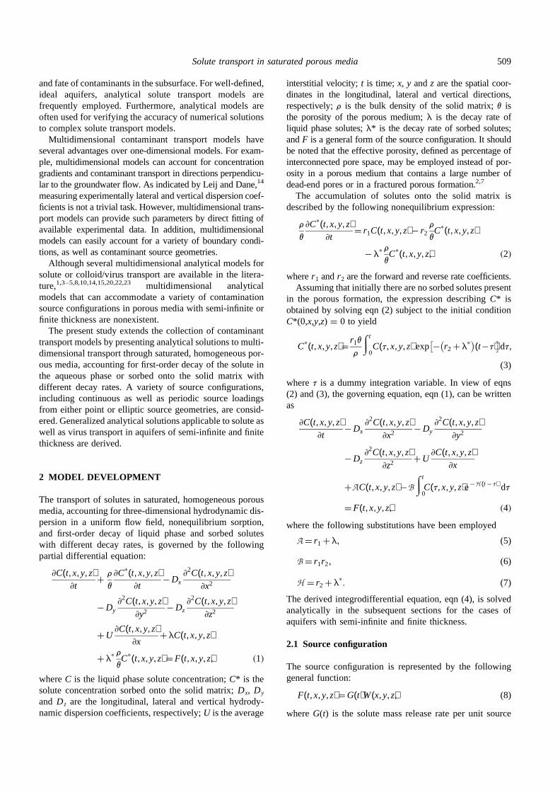
The appropriate initial and boundary conditions for the caseof an aquifer with infinite longitudinal and lateral directionsand semi-infinite vertical direction (thickness), as illustratedschematically in Fig. 1(a), are as follows:

C(0,x,y,z) ¼ 0, (11)

C(t, 6 `, y, z) ¼ 0, (12)

C(t,x, 6 `, z) ¼ 0, (13)

]C(t,x,y, 0)]z

¼ 0, (14)

]C(t,x,y, `)]z

¼ 0, (15)

where condition (11) corresponds to the situation in whichsolutes are initially absent from the three-dimensional por-ous formation, eqns (12) and (13) indicate that the aquiferis infinite horizontally and laterally, boundary condition(14) represents a zero dispersive flux boundary and eqn

(15) preserves concentration continuity for a semi-infinitevertical aquifer thickness. The vertical levelz ¼ 0 definesthe location of the water table or a confining layer. Eqn (4),subject to conditions (11)–(15), is solved analytically. Itshould be noted thatz increases in the downward direction.

The analytical solution to the governing partial differen-tial equation, eqn (4), can be derived by a variety of meth-ods, including the conventional method of separation ofvariables, as well as integral transform methods. Further-more, a solution technique developed by Walker24 invol-ving a Green function (fundamental solution) can also beutilized. However, in the present study, integral transformtechniques were employed because the multidimensionalmodels developed are an extension of our previous analy-tical work on virus transport models,19,20 where Laplacetransform techniques were employed. Similar mathematicaltechniques were employed for the analytical solutions ofmultidimensional solute transport by Torideet al.21 andShan and Javandel.18

Taking Laplace transforms with respect to time variabletand space variablez, and Fourier transforms with respect tospace variablesx andy of eqn (4), and subsequently employ-ing the transformed initial and boundary conditions,followed by inverse transformations, yields the desired ana-lytical solution for an aquifer with semi-infinite thickness

Fig. 1. Schematic illustration of point and elliptic sources of con-tamination with coordinateslx0

, ly0, lz0

in an aquifer with semi-infinite (a) and finite (b) thickness. Note that the positive direction

for the vertical coordinate is inverted.

510 Y. Sim and C.V. Chrysikopoulos

(see Appendix A):

C(t,x,y,z) ¼1

64p3DxDyDz

� �1=2 ∫t

0

∫`

¹ `

∫`

¹ `

∫`

0

3 F(t ¹ t,q, v, p)L1(t)

3∫t

0

L2(t)z3=2 L3(z,x¹ q, y¹ v) L4(z,zþ p)

��þ L4(z,z¹ p)ÿ dz þ

L3(t,x¹ q, y¹ v)t3=2

3 L4(t, zþp)þL4(t,z¹ p)� ��

dp dv dq dt,

ð16Þ

wherep, q, v and z are dummy integration variables; thefollowing definitions were employed:

L1(t) ¼ exp ¹ H t½ ÿ, (17a)

L2(t) ¼Bz

t ¹ z

� �1=2

I1 2 Bz(t ¹ z)ÿ �1=2

h i, (17b)

L3(t,x,y) ¼ expUx2Dx

¹14t

x2

Dxþ

y2

Dy

� ��

¹ t A ¹ H þU2

4Dx

� ��, ð17cÞ

L4(t,z) ¼ exp¹ z2

4Dzt

� �, (17d)

and I 1 is the modified Bessel function of the first kind offirst order.

2.2.1 Point source geometrySubstituting eqns (8) and (9) into eqn (16) yields the analy-tical solution for the case of point source geometry:

C(t,x,y,z) ¼1

64p3DxDyDz

� �1=2 ∫t

0

G(t ¹ t)v

L1(t)

3∫t

0

L2(t)z3=2 L3(z,x¹ lx0

,y¹ ly0)

�3

�L4(z,zþ lz0

) þ L4(z, z¹ lz0)�

dz

þL3(t,x¹ lx0

, y¹ ly0)

t3=2

3 L4(t,zþ lz0) þL4(t,z¹ lz0

)� ��

dt, ð18Þ

where L1–L4 are defined in eqns (17a)– (17d), respec-tively, and the following property of the Dirac delta func-tion was employed:∫b

af0(t)d(t ¹ t0) dt ¼ f0(t0), a # t0 # b, (19)

wherea andb are arbitrary constants, andf0 is an arbitraryfunction.

2.2.2 Elliptic source geometrySubstituting eqns (8) and (10) into eqn (16) leads to theanalytical solution for the case of elliptic source geometry:

C(t,x,y, z) ¼1

64p2DxDz

� �1=2 ∫t

0

∫a2

a1

G(t ¹ t)v

L1(t)

3∫t

0

L2(t)z

L3(z, x¹ q,0) L4(z, zþ lz0)

��þL4(z, z¹ lz0

)ÿL5(z) dz þL3(t,x¹ q,0)

t

3 L4(t, zþ lz0)þL4(t,z¹ lz0

)� �

L5(t)�

dq dt,

ð20Þ

whereL1–L4 are defined in eqns (17a)– (17d), respectively,

L5(t) ¼ erf k1(t,q,y)� �

¹ erf k2(t,q,y)� �

, (21)

a1 ¼ lx0¹ a, (22)

a2 ¼ lx0þ a, (23)

k1(t,q,y) ¼ y¹ ly0þ b2 ¹

b2(q¹ lx0)2

a2

" #1=2( )1

4Dyt

� �1=2

,

(24)

k2(t,q,y)¼ y¹ ly0¹ b2 ¹

b2(q¹ lx0)2

a2

" #1=2( )1

4Dyt

� �1=2

,

(25)

erf[·] is the error function, and the following transformationand integral relationships were employed:

k ¼y¹ v

(4tDy)1=2 (26a)

dk ¼¹ dv

(4tDy)1=2, (26b)

∫k2

k1

exp[ ¹ k2] dk ¼¹p1=2

2erf k1

� �¹ erf k2

� �� : (27)

As noted by Chrysikopoulos,4 solving for an elliptic sourcegeometry is advantageous because the appropriate solutionfor a circular source can easily be obtained by settinga ¼ b¼ r in eqns (22)–(25), wherer is the radius of the circularsource.

2.3 Aquifer with finite thickness

The desired analytical solution for the case of an aquiferwith finite thickness, as illustrated schematically in Fig.1(b), is obtained by solving eqn (4) subject to conditions(11)–(14) and the following finite vertical, lower boundarycondition:

]C(t,x, y, H)]z

¼ 0, (28)

whereH is the aquifer thickness. The boundary condition

Solute transport in saturated porous media 511

(28) implies that the aquifer is confined by an impermeablelayer at depthz ¼ H. Taking the Laplace transform withrespect to the time variablet, Fourier transforms withrespect to space variablesx and y, and the finite Fouriercosine transform with respect to the space variablez of eqn(4), and subsequently employing the transformed initial andboundary conditions, followed by inverse transformationsyields (see Appendix B):

C(t,x,y, z) ¼1

16p2DxDy

� �1=2 ∫t

0

∫`

¹ `

∫`

¹ `L1(t)

3∫t

0

L2(t)z

L3(z, x¹ q,y¹ v)�

3 L6 z, F̈(t ¹ t,q,v,0), F̈(t ¹ t, q,v,wm)ÿ �

dz

þL3(t,x¹ q, y¹ v)

tL6 t, F̈(t¹t,q,v,0),ÿ

3 F̈(t ¹ t,q, v,wm)Þ�

dv dq dt, ð29Þ

whereL1–L3 are defined in eqns (17a)–(17c), respectively,

L6(t, f1, f2) ¼f1H

þ2H

∑̀m¼ 1

f2 exp ¹ w2mDzt

� �cos wmzÿ �

,

(30)

wm ¼mp

H, (31)

m is the integer summation index,F̈(t,x, y,wm) representsthe finite Fourier cosine transform ofF(t,x,y,z) with respectto space variablez with corresponding finite Fourier cosinetransform variablewm, andf1 andf2 are arbitrary functions.

2.3.1 Point source geometryThe desired analytical solution for the case of point sourcegeometry is obtained by substituting the correspondingexpression for̈F(t,x, y,wm) into eqn (29). Substituting eqn(9) into eqn (8) and subsequently taking the finite Fouriercosine transform (defined in eqn (B3)) with respect to spacevariablez of the resulting expression yields

F̈(t, x,y,wm) ¼

∫H

0

G(t)v

d(x¹ lx0)d(y¹ ly0

)d(z¹ lz0)

3 cos(wmz) dz¼G(t)v

d(x¹ lx0)d(y¹ ly0

)

3 cos(wmlz0), ð32Þ

where the latter formulation in eqn (32) is a consequence ofemploying eqn (19). In view of eqns (19) and (32), thegeneral solution, eqn (29), reduces to the following form:

C(t,x,y,z) ¼1

16p2DxDy

� �1=2 ∫t

0

G(t ¹ t)v

L1(t)

3∫t

0

L2(t)z

L3(z,x¹ lx0,y¹ ly0

)�

3 L6 z,1, cos wmlz0

ÿ �ÿ �dz

þL3(t,x¹ lx0

, y¹ ly0)

t

3 L6 t, 1,cos wmlz0

ÿ �ÿ ��dt, ð33Þ

whereL1–L3 andL6 are defined in eqns (17a)–(17c) and(30), respectively.

2.3.2 Elliptic source geometryIn view of eqn (10), the finite Fourier cosine transform ofeqn (8) with respect toz is given by

F̈(t,x,y,wm)¼G(t)v

cos(wmlz0)

(x¹ lx0)2

a2 þ(y¹ ly0

)2

b2 #1,

0 otherwise:

8><>:(34)

Substituting eqn (34) into eqn (29), the desired analyticalsolution for the case of elliptic source geometry is asfollows:

C(t,x,y, z) ¼1

16pDx

� �1=2 ∫t

0

∫a2

a1

G(t ¹ t)v

L1(t)

3∫t

0

L2(t)z1=2 L3(z, x¹ q,0)L5(z)

�3 L6 z, 1,cos wmlz0

ÿ �ÿ �dzþ

L3(t, x¹ q,0)t1=2

3 L5(t)L6 t,1,cos wmlz0

ÿ �ÿ ��dq dt, ð35Þ

wherea1 anda2 are defined in eqns (22) and (23), respec-tively, andL1–L3, L5 and L6 are defined in eqns (17a)–(17c), (21) and (30), respectively.

3 MODEL SIMULATIONS AND DISCUSSION

Model simulations are performed for two different sourceconfigurations, and aquifers with either semi-infinite orfinite thickness. The integrals present in the analytical solu-tions (18), (20), (33) and (35) are evaluated numerically bythe integration routines Q1DA and QDAG, which utilizeglobally adaptive quadrature algorithms.11,12 The infiniteseries part of the solution for the case of an aquifer withfinite thickness (eqn (30)) is evaluated by considering up to1000 terms (m¼ 1000). The number of terms,m, is selectedso that additional terms do not alter the summation morethan 0.001%.

The groundwater table and the bottom of the finite thick-ness aquifer are assumed to be located atz¼ 0 cm andz¼ H¼ 100 cm, respectively. Although all analytical solutionsderived here are general enough to account for temporally

Table 1. Model parameters for simulations

Parameter Value Reference

Dx 1331.25 cm2 h¹1 Batu1

Dy ¼ Dz 268.75 cm2 h¹1 Batu1

U 0.625 cm h¹1 Batu1

l ¼ l* 0 days —r 1.5 g cm¹3 Yates and Ouyang25

v 0.25 Parket al.16

512 Y. Sim and C.V. Chrysikopoulos

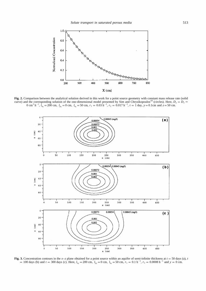
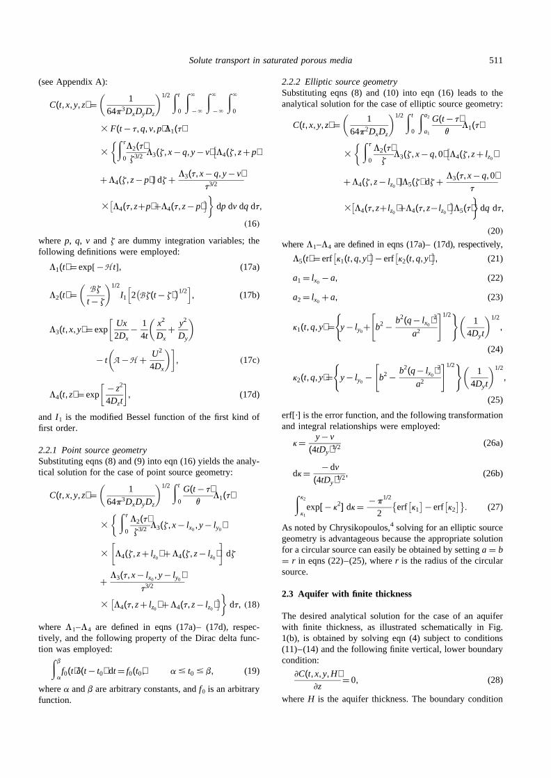
Fig. 2. Comparison between the analytical solution derived in this work for a point source geometry with constant mass release rate (solidcurve) and the corresponding solution of the one-dimensional model presented by Sim and Chrysikopoulos19 (circles). Here,Dy ¼ Dz .

0 cm2 h¹1, lx0¼ 200 cm, ly0

¼ 0 cm, lz0¼ 50 cm,r 1 ¼ 0.03 h¹1, r 2 ¼ 0.017 h¹1, t ¼ 1 day,y¼ 0:1cm andz¼ 50 cm.

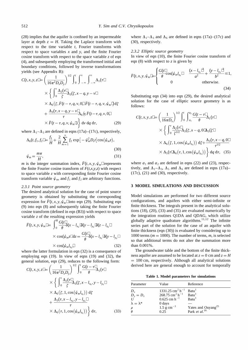
Fig. 3. Concentration contours in thex–z plane obtained for a point source within an aquifer of semi-infinite thickness att ¼ 50 days (a),t¼ 100 days (b) andt ¼ 300 days (c). Here,lx0

¼ 200 cm, ly0¼ 0 cm, lz0

¼ 50 cm,r 1 ¼ 0.1 h¹1, r 2 ¼ 0.0008 h¹1 andy ¼ 0 cm.

Solute transport in saturated porous media 513

periodic source loading, for simplicity, the model simula-tions presented are based on a constant solute mass releaserate and the value ofG is set to unity. Unless otherwisespecified, the fixed parameter values used in the simulationsare those listed in Table 1.

For the case whereDy ¼ Dz . 0 cm2 h¹1, the analyticalsolution derived in this work for a point source geometrywith constant solute mass release rate is equivalent to theone-dimensional analytical solution for virus transport withconstant concentration boundary conditions presented bySim and Chrysikopoulos19 (eqn (31)). For this specialcase, model simulations are compared in Fig. 2 against theone-dimensional model derived by Sim and Chrysikopou-los.19 It should be noted, however, that in Fig. 2 the con-centrations simulated by the one-dimensional transportmodel (circles) are normalized with the source concentra-tion (C0), whereas concentrations generated by solutionsderived in this work (solid curves) are normalized withthe steady-state concentration (C`) evaluated at t ¼

400 days, as suggested by Hunt.10 Fig. 2 clearly indicates

that the model simulations compared are virtuallyidentical.

Fig. 3 illustrates two-dimensional snapshots of soluteconcentration at three successive times simulated for anaquifer with semi-infinite thickness (eqn (18)). A pointsource is assumed to be located inside the aquifer atlx0

¼ 200 cm, ly0¼ 0 cm andlz0

¼ 50 cm. It is observedthat as the solute plume spreads with increasing time,solute spreading is restricted at the groundwater table (z ¼

0 cm), with a consequent zero gradient of solute concentra-tion distribution, whereas a continuous solute spreadingoccurs anywhere else below the water table because theaquifer extends to infinity without a boundary (eqn (15)).Consequently, the observed solute plume is asymmetricwith respect to the flow direction along the plume center-line. In contrast, Fig. 4 illustrates symmetric solute plumesat three successive times, for an aquifer with finite thicknessand point source geometry (eqn (33)). This is due to thepresence of a fixed impermeable lower boundary (eqn(28),z¼ H ¼ 100 cm) in addition to the upper groundwater

Fig. 4. Concentration contours in thex–z plane obtained for a point source within an aquifer of finite thickness att ¼ 50 days (a),t ¼100 days (b) andt ¼ 300 days (c). Here,lx0

¼ 200 cm, ly0¼ 0 cm, lz0

¼ 50 cm,r 1 ¼ 0.03 h¹1, r 2 ¼ 0.017 h¹1 andy ¼ 0 cm.

514 Y. Sim and C.V. Chrysikopoulos

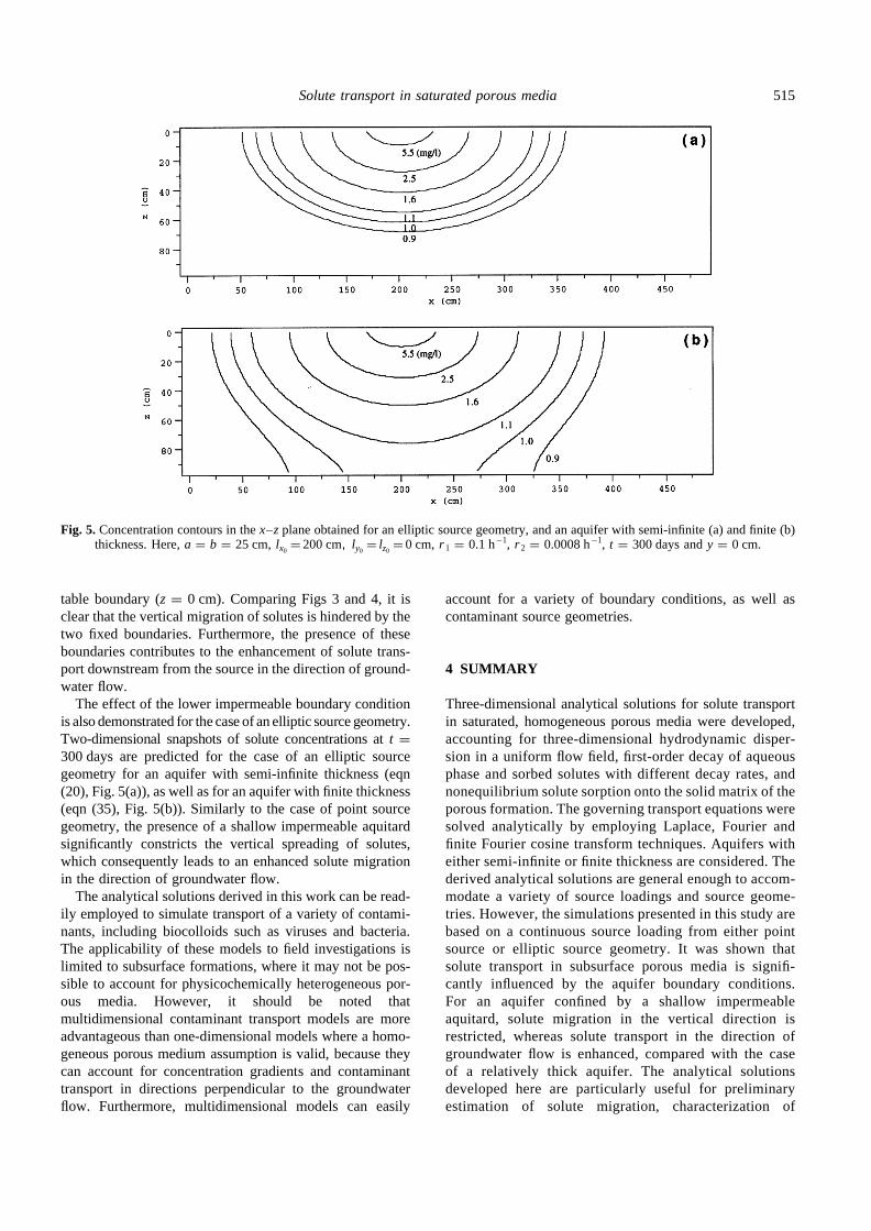
table boundary (z ¼ 0 cm). Comparing Figs 3 and 4, it isclear that the vertical migration of solutes is hindered by thetwo fixed boundaries. Furthermore, the presence of theseboundaries contributes to the enhancement of solute trans-port downstream from the source in the direction of ground-water flow.

The effect of the lower impermeable boundary conditionis also demonstrated for the case of an elliptic source geometry.Two-dimensional snapshots of solute concentrations att ¼

300 days are predicted for the case of an elliptic sourcegeometry for an aquifer with semi-infinite thickness (eqn(20), Fig. 5(a)), as well as for an aquifer with finite thickness(eqn (35), Fig. 5(b)). Similarly to the case of point sourcegeometry, the presence of a shallow impermeable aquitardsignificantly constricts the vertical spreading of solutes,which consequently leads to an enhanced solute migrationin the direction of groundwater flow.

The analytical solutions derived in this work can be read-ily employed to simulate transport of a variety of contami-nants, including biocolloids such as viruses and bacteria.The applicability of these models to field investigations islimited to subsurface formations, where it may not be pos-sible to account for physicochemically heterogeneous por-ous media. However, it should be noted thatmultidimensional contaminant transport models are moreadvantageous than one-dimensional models where a homo-geneous porous medium assumption is valid, because theycan account for concentration gradients and contaminanttransport in directions perpendicular to the groundwaterflow. Furthermore, multidimensional models can easily

account for a variety of boundary conditions, as well ascontaminant source geometries.

4 SUMMARY

Three-dimensional analytical solutions for solute transportin saturated, homogeneous porous media were developed,accounting for three-dimensional hydrodynamic disper-sion in a uniform flow field, first-order decay of aqueousphase and sorbed solutes with different decay rates, andnonequilibrium solute sorption onto the solid matrix of theporous formation. The governing transport equations weresolved analytically by employing Laplace, Fourier andfinite Fourier cosine transform techniques. Aquifers witheither semi-infinite or finite thickness are considered. Thederived analytical solutions are general enough to accom-modate a variety of source loadings and source geome-tries. However, the simulations presented in this study arebased on a continuous source loading from either pointsource or elliptic source geometry. It was shown thatsolute transport in subsurface porous media is signifi-cantly influenced by the aquifer boundary conditions.For an aquifer confined by a shallow impermeableaquitard, solute migration in the vertical direction isrestricted, whereas solute transport in the direction ofgroundwater flow is enhanced, compared with the caseof a relatively thick aquifer. The analytical solutionsdeveloped here are particularly useful for preliminaryestimation of solute migration, characterization of

Fig. 5. Concentration contours in thex–z plane obtained for an elliptic source geometry, and an aquifer with semi-infinite (a) and finite (b)thickness. Here,a ¼ b ¼ 25 cm, lx0

¼ 200 cm, ly0¼ lz0

¼ 0 cm, r 1 ¼ 0.1 h¹1, r 2 ¼ 0.0008 h¹1, t ¼ 300 days andy ¼ 0 cm.

Solute transport in saturated porous media 515

contamination sources, examination of possible aquiferboundary conditions, validation of numerical solutionsand determination of solute transport parameters fromlaboratory or well-defined field experiments.

ACKNOWLEDGEMENTS

This work was sponsored jointly by the National WaterResearch Institute and the University of California, WaterResources Center, as part of Water Resources Center Pro-ject UCAL-WRC-854. The content of this manuscript doesnot necessarily reflect the views of the agencies and noofficial endorsement should be inferred.

REFERENCES

1. Batu, V. A generalized two-dimensional analytical solutetransport model in bounded media for flux-type finitemultiple sources.Water Resour. Res., 1993, 29(8), 1125–1132.

2. Bear, J.,Dynamics of Fluids in Porous Media. Dover, 1972.3. Bellin, A., Rinaldo, A., Bosma, W. J. P., van der Zee, S. E. A.

T. M. and Rubin, Y. Linear equilibrium adsorbing solutetransport in physically and chemically heterogeneousporous formations. 1. Analytical solutions.Water Resour.Res., 1993,29(12), 4019–4030.

4. Chrysikopoulos, C. V. Three-dimensional analytical modelsof contaminant transport from nonaqueous phase liquid pooldissolution in saturated subsurface formations.Water Resour.Res., 1995,31(4), 1137–1145.

5. Chrysikopoulos, C. V., Voudrias, E. A. and Fyrillas, M. M.Modeling of contaminant transport resulting from dissolutionof nonaqueous phase liquid pools in saturated porous media.Trans. Porous Media, 1994,16(2), 125–145.

6. Churchill, R. V., Operational Mathematics. McGraw-Hill,New York, 1958.

7. Domenico, P. A. & Schwartz, F. W.,Physical and ChemicalHydrogeology. John Wiley, New York, 1990.

8. Goltz, M. N. and Roberts, P. V. Three-dimensional solutionsfor solute transport in an infinite medium with mobile andimmobile zones.Water Resour. Res., 1986, 22(7), 1139–1148.

9. Gradshteyn, I. S. & Ryzhik, I. M.,Table of Integral, Series,and Products. Academic Press, New York, 1980.

10. Hunt, B. Dispersive sources in uniform groundwater flow.J.Hydraul. Div., Am. Soc. Civ. Engng, 1978,104(HY1), 75–85.

11. IMSL, IMSL MATH/LIBRARY User’s Manual, version 2.0.IMSL, Houston, 1991.

12. Kahaner, D., Moler, C. & Nash, S.,Numerical Methods andSoftware. Prentice Hall, Englewood Cliffs, NJ, 1989.

13. Kreyszig, E.,Advanced Engineering Mathematics, 7th ed.John Wiley, New York, 1993.

14. Leij, F. J. and Dane, J. H. Analytical solutions of the one-dimensional advection equation and two- or three-dimensional dispersion equation.Water Resour. Res., 1990,26(7), 1475–1482.

15. Leij, F. J., Skaggs, T. H. and van Genuchten, M. Th.Analytical solutions for solute transport in three-dimensionalsemi-infinite porous media.Water Resour. Res., 1991,27(10), 2719–2733.

16. Park, N., Blanford, T. N. & Huyakorn, P. S.,VIRALT: AModular Semi-analytical and Numerical Model forSimulating Viral Transport in Ground Water. International

Ground Water Modeling Center, Colorado School of Mines,Golden, CO, 1992.

17. Roberts, G. E. & Kaufman, H.,Table of Laplace Transforms.W. B. Saunders, Philadelphia, PA, 1966.

18. Shan, C. and Javandel, I. Analytical solutions for solutetransport in a vertical aquifer section.J. Contam. Hydrol.,1997,27(1)2, 63–82.

19. Sim, Y. & Chrysikopoulos, C. V., Analytical models for one-dimensional virus transport in saturated porous media.WaterResour. Res., 31(5) (1995) 1429–1437. [Correction,WaterResour. Res., 32(5), (1996) 1473].

20. Sim, Y. and Chrysikopoulos, C. V. Three-dimensionalanalytical models for virus transport in saturated porousmedia.Transport in Porous Media, 1998,30(1), 87–112.

21. Toride, N., Leij, F. J. and Van Genuchten, M. T. Acomprehensive set of analytical solutions fornonequilibrium solute transport with 1st-order decayand zero-order production.Water Resour. Res., 1993,29(7), 2167–2182.

22. van Dujin, C. J. and van der Zee, S. E. A. T. M. Solutetransport parallel to an interface separating two differentporous materials.Water Resour. Res., 1986,22(13), 1779–1789.

23. van Kooten, J. J. A. A method to solve the advection–dispersion equation with a kinetic adsorption isotherm.Adv. Water Resour., 1996,19(4), 193–206.

24. Walker, G. R. Solution to a class of coupled linearpartial differential equations.IMA J. Appl. Math.,1987,38, 35–48.

25. Yates, M. V. and Ouyang, Y. VIRTUS, a model of virustransport in unsaturated soils.Appl. Environ. Microb.,1992,58(5), 1609–1616

APPENDIX A DERIVATION OF THE ANALYTICALSOLUTION FOR AN AQUIFER WITH SEMI-INFINITE THICKNESS

The analytical solution for the case of semi-infinite thick-ness is obtained by solving eqn (4) subject to conditions(11)–(15). Taking Laplace transforms with respect to timevariablet and space variablez, and Fourier transforms withrespect to space variablesx and y of eqn (4) and subse-quently employing eqn (11) and transformed boundarycondition (14) yields

C̃(s,g,q,f) ¼f

¯̂̃C(s,g,q, 0)

(f þ E)(f ¹ E)¹

˙̂̄F̃(s,g,q,f)

Dz(f þ E)(f ¹ E),

(A1)

where

E ¼1

D1=2z

sþ g2Dx þ igU þ q2Dy þ A ¹B

sþ H

� �1=2

,

(A2)

and the following properties were employed for the Laplaceand Fourier transformations:13,17

C̃(s,x,y,z) ¼

∫`

0C(t,x,y,z)e¹ st dt, (A3)

ˆ̃C(s,g, y, z) ¼1

(2p)1=2

∫`

¹ `C̃(s,x,y,z)e¹ igx dx, (A4)

516 Y. Sim and C.V. Chrysikopoulos

¯̂̃C(s,g,q,z) ¼

1(2p)1=2

∫`

¹ `

ˆ̃C(s,g, y, z)e¹ iqy dy, (A5)

˙̂̄C̃(s,g,q,f) ¼

∫`

0

¯̂̃C(s,g,q, z)e¹fz dz, (A6)

where the tilde and overdot signify Laplace transform withrespect to time and space variablest and z, respectively,and s and f are the corresponding Laplace domain vari-ables; the hat and overbar signify Fourier transforms withrespect to space variablesx and y with correspondingFourier domain variablesg and q, respectively; andi ¼ ( ¹ 1)1/2.

Taking the Laplace inverse transformation of eqn (A1)with respect tof, applying boundary condition (15) and

subsequently evaluating¯̂̃C(s,g,q,0) at the limit z → `,

yields

¯̂̃C(s,g,q,z) ¼

12Dz

∫`

0

¯̂̃F(s,g,q,p) F(s,g,q,zþ p)

��þ F(s,g,q,p¹ z)ÿ dpþ

∫z

0

¯̂̃F(s,g,q,p)

3 F(s,g,q,z¹ p) ¹ F(s,g,q,p¹ z)� �

dp

�,

ðA7Þwhere

F(s,g,q, z) ¼e¹ Ez

E, (A8)

and the following Laplace inversion identities were uti-lized:17

L ¹ 1 f̃ 1(p)f̃ 2(p)�

¼

∫z

0f1(z¹ p)f2(p) dp, (A9)

L ¹ 1 f

(f þ a)(f þ b)

� �¼

ae¹ az

a ¹ bþ

be¹ bz

b¹ a, (A10)

L ¹ 1 1(f þ a)(f þ b)

� �¼

e¹ az ¹ e¹bz

b¹ a, (A11)

whereL¹1 is the Laplace inverse operator, anda andb arearbitrary constants.

Furthermore, for mathematical convenience, let

F ¼HF

sþ Hþ

sFsþ H

: (A12)

The inverse Laplace transformation of eqn (A12) withrespect tos can be found by employing the followingrelationship:19

L ¹ 1 1sþ H

f̃ 0 sþ H ¹a

sþ H

� �� �¼ e¹ H t

∫t

0I0 2 az(t ¹ z)

ÿ �1=2h i

f0(z) dz, ðA13Þ

where f̃ 0(s) is the Laplace transform of the arbitrary func-tion f0(t) anda is an arbitrary constant. Following the pro-cedures provided in Sim and Chrysikopoulos,19 the inverse

Laplace transform of eqn (A12) is obtained as

L¹ 1 HF(s,g,q, z)sþ H

þsF

sþ H

� �

¼ H ¯̂P(t,g,q,z) þ] ¯̂P(t,g,q, z)

]t, ðA14Þ

where

¯̂P(t,g,q,z) ¼ e¹ H t∫t

0I0 2 Bz(t ¹ z)

ÿ �1=2h i Dz

pz

� �1=2

3 exp ¹z2

4Dzz¹ q2Dy þ A ¹ Hÿ �

z

� �Q (g, z) dz,

ðA15Þ

] ¯̂P(t,g,q,z)]t

¼ e¹ H t∫t

0

Bz

t ¹ z

� �1=2

I1 2 Bz(t ¹ z)ÿ �1=2

h i�¹ H I0 2 Bz(t ¹ z)

ÿ �1=2h i

g 3Dz

pz

� �1=2

3 exp ¹z2

4Dzz¹ q2Dy þ A ¹ Hÿ �

z

� �3 Q (g, z) dz þ e¹ H t Dz

pt

� �1=2

3 exp ¹z2

4Dzt¹ q2DyþA¹Hÿ �

t

� �Q (g, t),

ðA16Þ

Q (g, t) ¼ exp ¹ Dxt g2 þiUDx

g

� �� �: (A17)

In view of eqns (A12) and (A14), and application of theconvolution theorem, the inverse Laplace transformation ofeqn (A7) with respect tos is given by

¯̂C(t,g,q,z) ¼1

2Dz

∫t

0

∫`

0

¯̂F(t ¹ t,g,q,p)�H ¯̂P(t,g,q, zþp)

þ] ¯̂P(t,g,q,zþ p)

]tþ H ¯̂P(t,g,q, p¹ z)

þ] ¯̂P(t,g,q,p¹ z)

]t

�dp dt: ðA18Þ

The inverse Fourier transformation of eqn (A18) withrespect tog is

C̄(t,x,q,z) ¼1

8pD2z

� �1=2 ∫t

0

∫`

¹ `

∫`

0F̄(t ¹ t,q,q,p)

3

�H P̄(t, x¹ q,q, zþ p)

þ]P̄(t,x¹ q,q,zþ p)

]t

þ HP̄(t,x¹ q,q,p¹ z)

þ]P̄(t,x¹ q,q,p¹ z)

]t

�dp dq dt, ðA19Þ

Solute transport in saturated porous media 517

where the following definitions of the Fourier inversetransform were employed:

F ¹ 1 f̂ 1(g)�

¼1

(2p)1=2

∫`

¹ `f̂ 1(g)eigx dg, (A20)

F ¹ 1 f̂ 1(g)f̂ 2(g)�

¼1

(2p)1=2

∫`

¹ `f1(x¹ y)f2(y) dy,

(A21)whereF¹1 is the Fourier inverse operator andy is a dummyintegration variable.

In order to obtain the inverse Fourier transformation ofeqn (A15) with respect tog, only the termQ(g,t) defined ineqn (A17) requires inversion, and is obtained as follows:

F ¹ 1 Q (g, t)�

¼1

(2p)1=2

∫`

¹ `exp ¹ Dxt g2 þ

iUDx

g

� �� �3 eigx dg¼

12Dxt

� �1=2

h(x, t), ðA22Þ

where

h(x, t) ¼ exp ¹1

Dx

U2t4

þx2

4t¹

Ux2

� �� �, (A23)

and the latter expression in eqn (A22) is a consequence ofemploying Euler’s formula (eigx ¼ cos(gx) þ isin(gx)) andthe integral identities found in Gradshteyn and Ryzhik9

(eqn 3.923.1 and 2, p. 485) were utilized. Therefore, inview of eqn (A22), the inverse Fourier transformation ofeqn (A15) is

P̄(t, x,q,z) ¼ e¹ H t∫t

0I0 2 Bz(t ¹ z)

ÿ �1=2h i Dz

2pDxz2

� �1=2

3 exp ¹z2

4Dzz¹ q2Dy þ A ¹ Hÿ �

z

��3 h(x, z) dz: ðA24Þ

The inverse Fourier transformation of eqn (A19) withrespect toq is

C(t,x,y,z) ¼1

4pDz

∫t

0

∫`

¹ `

∫`

¹ `

∫`

0F(t ¹ t, q,v,p)

3

�HP(t,x¹ q, y¹ v, zþ p)

þ]P(t,x¹ q, y¹ v,zþ p)

]t

þ H P(t, x¹ q,y¹ v,p¹ z)

þ]P(t,x¹ q, y¹ v,p¹ z)

]t

�dp dv dq dt:

ðA25Þ

In view of the following inverse Fourier transform relation-ship (see Kreryszig,13 eqn 9, p. 621):

F ¹ 1 exp ¹ q2Dyz� ��

¼1

2Dyz

� �1=2

exp ¹y2

4Dyz

� �,

(A26)

the inverse Fourier transformation of eqn (A24) is

P(t,x,y,z) ¼ e¹ H t∫t

0I0 2 Bz(t ¹ z)

ÿ �1=2h i Dz

4pDxDyz3

� �1=2

3 exp ¹z2

4Dzz¹

y2

4Dyz¹ A ¹ Hð Þz

� �3 h(x, z) dz: ðA27Þ

Furthermore, in order to complete the description of eqn(A25), the derivative ofP(t,x,y,z) with respect to t isobtained as follows:

]P(t,x,y,z)]t

¼ e¹ H t∫t

0

Bz

t ¹ z

� �1=2

I1 2 Bz(t ¹ z)ÿ �1=2

h i�¹ H I0 2 Bz(t ¹ z)

ÿ �1=2h io

3Dz

4pDxDyz3

� �1=2

3 exp ¹z2

4Dzz¹

y2

4Dyz¹ A ¹ Hð Þz

� �

3 h(x, z) dz þ e¹ H t Dz

4pDxDyt3

� �1=2

3 exp ¹z2

4Dzt¹

y2

4Dyt¹ A ¹ Hð Þt

� �h(x, t):

ðA28Þ

Substituting eqn (A23) into eqns (A27) and (A28) and sub-sequently substituting the resulting expressions into eqn(A25) yields the desired generalized analytical solution,eqns (16), (17a)– (17d).

APPENDIX B DERIVATION OF THE ANALYTICALSOLUTION FOR AN AQUIFER WITH FINITETHICKNESS

The analytical solution for the case of an aquifer with finitethickness is obtained by solving eqn (4) subject to eqns(11)–(14) and (28). Taking the Laplace transform withrespect to the time variablet, Fourier transforms withrespect to space variablesx and y, and the finite Fouriercosine transform with respect to space variablez of eqn(4) and subsequently employing transformed initial condi-tion (11) yields

¨̄̂C̃(s,g,q,wm) ¼

¨̄̂F̃(s,g,q,wm)

g2Dx þ igU þ E, (B1)

where

E¼q2Dy þ w2mDz þ A þ s¹

Bsþ H

, (B2)

the Laplace and Fourier transformation properties (A3)–(A5),and the following finite Fourier cosine transformation and

518 Y. Sim and C.V. Chrysikopoulos

operational property were employed (see Churchill,6 p. 294):

¨̄̂C̃(s,g,q,wm) ¼

∫H

0

¯̂̃C(s,g,q,z)cos(wmz) dz, (B3)

F fcd2f (z)dz2

� �¼ w2

mf̈ (w2m) ¹

df (0)dz

þ ( ¹ 1)m df̈ (H)dz

(m¼ 0,1,2…), ðB4Þ

where the double over-dot signifies finite Fourier cosinetransform with respect to space variablez, withcorresponding finite Fourier cosine transform variablewm

¼ mp/H, F fc is the finite Fourier cosine transform operatorand f is an arbitrary function.

The Fourier inverse transformation of eqn (B1) withrespect tog is obtained by employing the Fourier inversetransforms (A20) and (A21), Euler’s formula, integralidentities found in Gradshteyn and Ryzhik9 (eqns 3.724.1and 2, p. 407), eqn (B2) and application of the convolutiontheorem as follows:

¨̄̃C(s,x,q,wm) ¼

∫`

¹ `

¨̄̃F(s, q,q,wm)W(s,x¹ q,q,wm) dq,

(B5)where

W(s, x,q,wm) ¼1

4DxDy q2 þ Sÿ � !1=2

expUx2Dx

� �

3 exp ¹ x q2 þ Sÿ �Dy

Dx

� �1=2� �, ðB6Þ

S ¼1

Dyw2

mDz þ A þ s¹B

sþ Hþ

U2

4Dx

� �: (B7)

In view of eqns (A20), (A21) and (B6), Euler’s formula, theintegral identity found in Gradshteyn and Ryzhik9 (eqn3.961.2, p. 498), and application of the convolutiontheorem, the inverse Fourier transformation of eqn (B5)with respect toq is given by

¨̃C(s,x,y,wm)¼∫`

¹ `

∫`

¹ `

¨̃F(s, q,v,wm)g(s,x¹q,y¹v,wm)dv dq,

(B8)

where

g(s,x,y,wm) ¼1

4p2DxDy

� �1=2

expUx2Dx

� �

3 K0 S1=2 y2 þ x2 Dy

Dx

� �1=2� �: ðB9Þ

In view of eqns (B7) and (B9), the inverse Laplace trans-form (see Roberts and Kaufman,17 eqn 3, p. 169 andeqn 13.2.1, p. 304):

f0(t) ¼ L ¹ 1 K0 b1 sþ b2

ÿ �1=2h in o

¼12t

exp¹b2

1

4t¹ b2t

� �,

(B10)

and by following the procedures outlined in Appendix A,the inverse Laplace transformation of eqn (B8) with respectto s is given by

C̈(t,x,y,wm) ¼1

16p2DxDy

� �1=2 ∫t

0

∫`

¹ `

∫`

¹ `

3 expU(x¹ q)

2Dx

� �e¹ HtF̈(t ¹ t,q, v,wm)

3∫t

0

Bz(t ¹ z)

� �1=2

I1 2 Bz(t ¹ z)ÿ �1=2

h i�3 exp ¹ z w2

mDz þ A þU2

4Dx¹ H

� �� �3 exp ¹

14z

(x¹ q)2

Dxþ

(y¹ v)2

Dy

� �� �dz

þ1t

exp ¹ t w2mDz þ A þ

U2

4Dx¹ H

� �� �3 exp ¹

14t

(x¹ q)2

Dxþ

(y¹ v)2

Dy

� �� ��3 dv dq dt: ðB11Þ

The inverse Fourier cosine transformation of eqn (B11)with respect towm is given by

C(t,x,y, z) ¼1

16p2DxDy

� �1=2 ∫t

0

∫`

¹ `

∫`

¹ `

3 expU(x¹ q)

2Dx

� �e¹ Ht

3∫t

0

Bz(t ¹ z)

� �1=2

I1 2 Bz(t ¹ z)ÿ �1=2

h i�3 exp ¹

14z

(x¹ q)2

Dxþ

(y¹ v)2

Dy

� �� �3 exp ¹ z A þ

U2

4Dx¹ H

� �� �3 F ¹ 1

fc F̈(t ¹ t,q, v,wm)exp ¹ w2mDzz

� �� dz

þ1texp ¹

14t

(x¹ q)2

Dxþ

(y¹ v)2

Dy

� �� �3 exp ¹ t A þ

U2

4Dx¹ H

� �� �3 F ¹ 1

fc F̈(t ¹ t,q, v,wm)exp ¹ w2mDzt

� �� �3 dv dq dt, ðB12Þ

where F ¹ 1fc is the inverse finite Fourier cosine operator,

defined as

F ¹ 1fc f̈ (wm)�

¼f̈ (0)H

þ2H

∑̀m¼ 1

f̈ (wm)cos(wmz), 0 # z# H:

(B13)In view of eqn (B13), eqn (B12) is simplified to the form ofthe generalized analytical solution, eqns (29)–(31).

Solute transport in saturated porous media 519