Analytical solutions for advective–dispersive solute transport in double-layered finite porous media

INTERNATIONAL JOURNAL FOR NUMERICAL AND ANALYTICAL METHODS IN GEOMECHANICSInt. J. Numer. Anal. Meth. Geomech. 2011; 35:438–460Published online 14 May 2010 in Wiley Online Library (wileyonlinelibrary.com). DOI: 10.1002/nag.903

Analytical solutions for advective–dispersive solute transportin double-layered finite porous media

Yu-Chao Li‡ and Peter John Cleall∗,†,§

Geoenvironmental Research Centre, Cardiff School of Engineering, Cardiff University,Cardiff, CF24 3AA, Wales, U.K.

SUMMARY

Analytical solutions for advection and dispersion of a conservative solute in a one-dimensional double-layered finite porous media are presented. The solutions are applicable to five scenarios that have variouscombinations of fixed concentration, fixed flux and zero concentration gradient conditions at the inlet andoutlet boundaries that provide a wide number of options. Arbitrary initial solute concentration distributionsthroughout the media can be considered via explicit formulations or numerical integration. The analyticalsolutions presented have been verified against numerical solutions from a finite-element-based approachand an existing closed-form solution for double-layered media with an excellent correlation being found inboth cases. A practical application pertaining to advective transport induced by consolidation of underlyingsediment layers on contaminant movement within a capped contaminated sediment system is presented.Comparison of the calculated concentrations and fluxes with alternative approaches clearly illustrates theneed to consider advection processes. Consideration of the different features of contaminant transportdue to varying pore-water velocity fields in primary consolidation and secondary consolidation stagesis achieved via the use of non-uniform initial concentration distributions within the proposed analyticalsolutions. Copyright � 2010 John Wiley & Sons, Ltd.

Received 3 June 2009; Revised 6 January 2010; Accepted 12 January 2010

KEY WORDS: advection; analytical techniques; containment; diffusion; layered systems; porous media

1. INTRODUCTION

Contaminant transport in layered porous media is often observed in geoenvironmental engineeringas stratified soils are formed by both geological sedimentation/weathering and anthropogenicactivities, such as construction of engineered barriers to contain contamination dispersions orremediation of the existing contaminated sites [1].

When considering advective and dispersive transport in layered soils, the medium is usuallyassumed to be a series of homogeneous layers, each having its own physical and chemical proper-ties, and with pore-water flow limited to being perpendicular to the layers. A simplifying approach[2, 3] for the concentration distribution in layered media was obtained by assuming that theconcentration in any layer is independent of the transport properties of the downstream layers.

∗Correspondence to: Peter John Cleall, Geoenvironmental Research Centre, Cardiff School of Engineering, CardiffUniversity, Cardiff, CF24 3AA, Wales, U.K.

†E-mail: [email protected]‡Research Associate.§Lecturer.

Contract/grant sponsor: Engineering and Physical Sciences Research Council, U.K.; contract/grant number:EP/C532651/2

Copyright � 2010 John Wiley & Sons, Ltd.

ANALYTICAL SOLUTIONS FOR ADVECTIVE–DISPERSIVE SOLUTE TRANSPORT 439

The concentration profile in each layer can be evaluated with the analytical solutions for homo-geneous media by applying a first- or third-type condition at the inlet boundary, at which theconcentration follows directly from the solute concentration of the upper layer, and a zero gradientat the outlet boundary. Some analytical solutions are also available for the consideration of advec-tion and dispersion of solutes in layered media. Leij et al. [4] proposed an approach to solvethe advection–dispersion equation (ADE) for a two-layer medium using Laplace transformationscombined with a numerical inversion transform. They addressed mass balance at the interfacebetween the layers by considering different interface continuity conditions. Leij and van Genuchten[5] presented approximate solutions for the ADE for a two-layer porous medium with a zeroconcentration initial condition using Laplace transformations and binomial theorem. The outletlayer was assumed to be of infinite thickness by both Leij et al. [4] and Leij and van Genuchten[5], and this assumption may lead to errors when a finite system is considered. Liu et al. [6]presented an analytical solution to the one-dimensional ADE in multi-layer porous media usinga generalized integral transform method. This solution is relatively complex, although it is ableto yield valuable insights into the key mechanisms. All of the aforementioned analytical solutionsonly consider scenarios with a third-type (or Robin) condition at the inlet boundary and a second-type (or Neumann) condition at the outlet boundary or infinity. Such combinations of boundaryconditions are not applicable for many practical geoenvironmental problems.

This paper presents analytical solutions for advective and dispersive solute transport in double-layered finite porous media subjected to arbitrary initial conditions. These solutions are presented interms of a combination of different inlet and outlet boundary conditions that provide a wide numberof options. These analytical solutions are able to offer insight into the governing physical processes,provide useful tools for validating numerical approaches and are often applicable to practicalproblems. They are also sometimes more computationally efficient, compared with numericalapproaches, and address the Robin-type boundary condition that is often not available in numericalprogrammes. The analytical solutions are verified against numerical solutions and are comparedwith an existing solution [5]. Finally, the influence of pore-water flow induced by underlyingsediment consolidation on contaminant transport within a capped contaminated sediment systemis evaluated as an example.

2. THEORY

2.1. Problem formulation

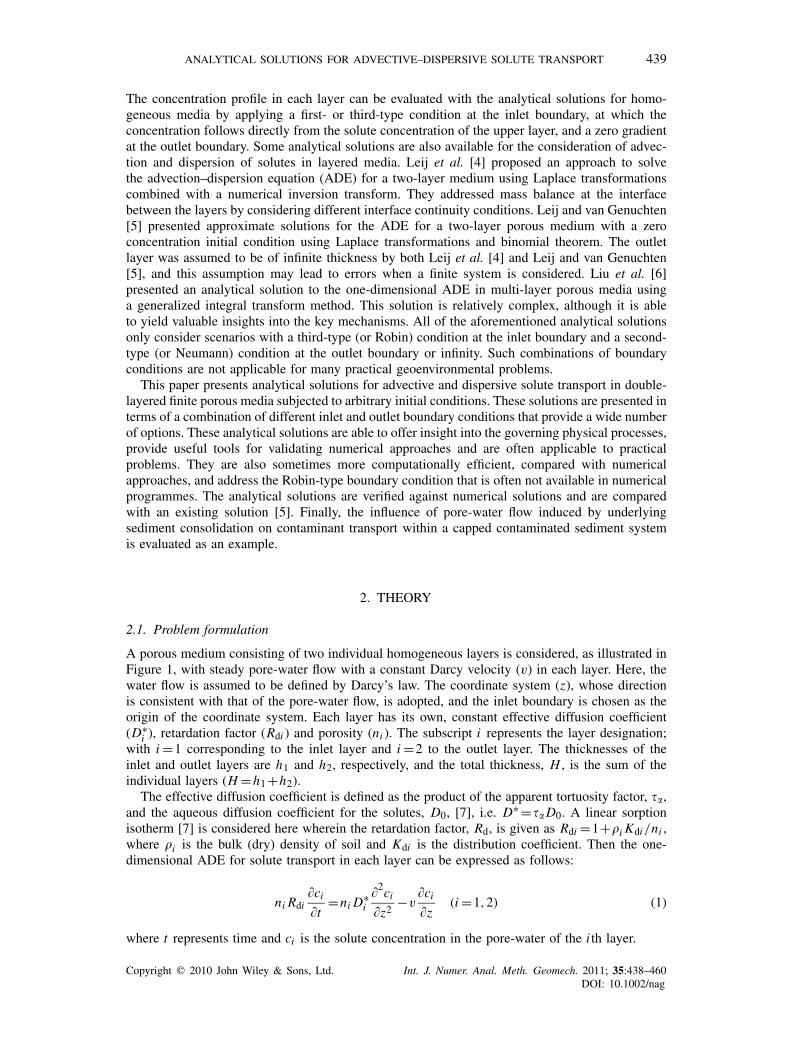
A porous medium consisting of two individual homogeneous layers is considered, as illustrated inFigure 1, with steady pore-water flow with a constant Darcy velocity (v) in each layer. Here, thewater flow is assumed to be defined by Darcy’s law. The coordinate system (z), whose directionis consistent with that of the pore-water flow, is adopted, and the inlet boundary is chosen as theorigin of the coordinate system. Each layer has its own, constant effective diffusion coefficient(D∗

i ), retardation factor (Rdi ) and porosity (ni ). The subscript i represents the layer designation;with i =1 corresponding to the inlet layer and i =2 to the outlet layer. The thicknesses of theinlet and outlet layers are h1 and h2, respectively, and the total thickness, H , is the sum of theindividual layers (H =h1 +h2).

The effective diffusion coefficient is defined as the product of the apparent tortuosity factor, ��,and the aqueous diffusion coefficient for the solutes, D0, [7], i.e. D∗ =��D0. A linear sorptionisotherm [7] is considered here wherein the retardation factor, Rd, is given as Rdi =1+�i Kdi/ni ,where �i is the bulk (dry) density of soil and Kdi is the distribution coefficient. Then the one-dimensional ADE for solute transport in each layer can be expressed as follows:

ni Rdi�ci

�t=ni D∗

i�2ci

�z2−v

�ci

�z(i =1,2) (1)

where t represents time and ci is the solute concentration in the pore-water of the i th layer.

Copyright � 2010 John Wiley & Sons, Ltd. Int. J. Numer. Anal. Meth. Geomech. 2011; 35:438–460DOI: 10.1002/nag

440 Y.-C. LI AND P. J. CLEALL

Figure 1. Schematic representation for advection–dispersion solute transport ina double-layered porous medium.

The pore-water velocity determined by Darcy’s law, sometimes termed as the effective orapparent velocity, has the same value for both the layers. The seepage velocity of water in the i thlayer, vsi , is equal to v/ni , and water mass balance at the interface between the layers is satisfieddue to the relationship of vs1n1 =vs2n2 =v. If vsi is substituted into Equation (1), it becomes thewidely used one-dimensional ADE [7, 8], i.e.

Rdi�ci

�t= D∗

i�2ci

�z2−vsi

�ci

�z(i =1,2) (2)

Arbitrary initial conditions are defined as follows:

ci (z, t)=ci (z,0) (i =1,2) (3)

where ci (z,0) is an arbitrary function for the initial solute concentration distribution in the i thlayer.

The inlet and outlet boundary conditions considered in this paper are as follows:

Inlet boundary: c1(0, t) = c0 (Dirichlet or first type) (4a)

or −n1 D∗1�c1(z, t)

�z

∣∣∣∣z=0

+vc1(0, t) = vc0 (Robin [9] or third type) (4b)

Outlet boundary: c2(H, t) = cH (Dirichlet or first type) (5a)

or�c2(z, t)

�z

∣∣∣∣z=H

= 0 (Neumann or second type) (5b)

or −n2 D∗2

�c2(z, t)

�z

∣∣∣∣z=H

+vc2(H, t) = vcH (Robin or third type) (5c)

where c0 and cH are the constant boundary solute concentrations at the inlet and outlet boundaries,respectively. Equations (4a) and (5a) represent fixed solute concentration situations, Equations (4b)and (5c) represent fixed flux situations and Equation (5b) is the zero gradient condition often usedto describe the outlet boundary [4–6].

A detailed discussion on the continuity conditions at the interface between the layers has beenmade by Leij et al. [4]. Simultaneous imposition of the Dirichlet and the Robin conditions at the



Table I. Scenarios with various combinations of inlet and outlet boundary conditions.

Scenario Inlet boundary Outlet boundary

Dirichlet inlet and outlet c1(0, t)=c0 c2(H, t)=cH

Dirichlet inlet–Neumann outlet c1(0, t)=c0�c2(z,t)

�z

∣∣z=H =0

Dirichlet inlet–Robin outlet c1(0, t)=c0 −n2 D∗2

�c2(z,t)�z

∣∣z=H +vc2(H, t)=vcH

Robin inlet–Dirichlet outlet −n1 D∗1

�c1(z,t)�z

∣∣∣ z=0 c2(H, t)=cH

+vc1(0, t)=vc0

Robin inlet–Neumann outlet −n1 D∗1

�c1(z,t)�z

∣∣∣z=0

�c2(z,t)�z

∣∣z=H =0

+vc1(0, t)=vc0

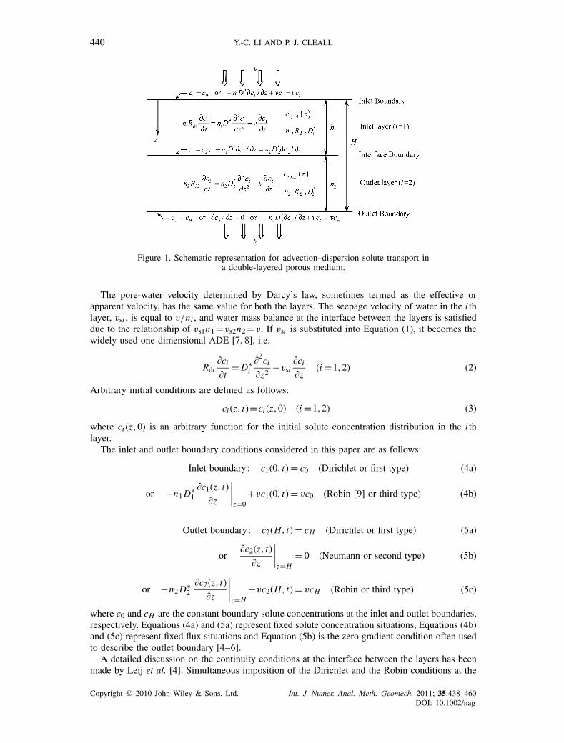
Figure 2. Potential application cases: (a) landfill liner system; (b) capped contaminated sediment system;and (c) vertical barrier system.

interface was found to ensure both solute concentration and solute flux continuities and provides asuperior description of the physical problem compared with when only one condition is satisfied.The Dirichlet and the Robin continuity conditions at the interface can be expressed as follows,respectively:

c1(h1, t)=c2(h1, t) (6a)

and

−n1 D∗1�c1(z, t)

�z

∣∣∣∣z=h1

+vc1(h1, t)=−n2 D∗2

�c2(z, t)

�z

∣∣∣∣z=h1

+vc2(h1, t) (6b)

Equation (6b) becomes a Neumann continuity condition after substitution of Equation (6a) yielding

n1 D∗1

�c1(z, t)

�z

∣∣∣∣z=h1

=n2 D∗2

�c2(z, t)

�z

∣∣∣∣z=h1

(7)

Analytical solutions for the governing equations, i.e. Equation (1), subjected to the initial condition,i.e. Equation (3), and the boundary conditions, i.e. Equations (4)–(6), are presented in this paper.A scenario with fixed flux conditions at both the inlet and the outlet boundaries is not includedsince such a system will not reach a steady-state if different fixed flux values are applied. However,the analytical solution for the scenario with zero flux conditions at both the inlet and the outletboundaries is worth consideration since this scenario may represent cases of contaminant releasefrom contaminated media. The analytical solutions presented in this paper for the scenarios listedin Table I can be applied to a number of geoenvironmental engineering applications as representedin Figure 2.



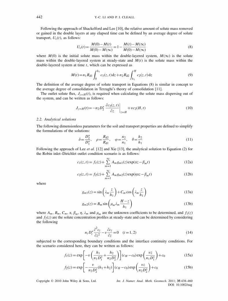
Following the approach of Shackelford and Lee [10], the relative amount of solute mass removedor gained in the double layers at any elapsed time can be defined by an average degree of solutetransport, Uc(t), as follows:

Uc(t)= M(0)− M(t)

M(0)− M(∞)=1− M(t)− M(∞)

M(0)− M(∞)(8)

where M(0) is the initial solute mass within the double-layered system, M(∞) is the solutemass within the double-layered system at steady-state and M(t) is the solute mass within thedouble-layered system at time t , which can be expressed as

M(t)=n1 Rd1

∫ h1

0c1(z, t)dz+n2 Rd2

∫ H

h1

c2(z, t)dz (9)

The definition of the average degree of solute transport in Equations (8) is similar in concept tothe average degree of consolidation in Terzaghi’s theory of consolidation [11].

The outlet solute flux, Jz=H (t), is required when calculating the solute mass dispersing out ofthe system, and can be written as follows:

Jz=H (t)=−n2 D∗2

�c2(z, t)

�z

∣∣∣∣z=H

+vc2(H, t) (10)

2.2. Analytical solutions

The following dimensionless parameters for the soil and transport properties are defined to simplifythe formulations of the solutions:

�= D∗2

D∗1, �= Rd2

Rd1, �= n2

n1, �= h2

h1(11)

Following the approach of Lee et al. [12] and Xie [13], the analytical solution to Equation (2) forthe Robin inlet–Dirichlet outlet condition scenario is as follows:

c1(z, t) = f1(z)+∞∑

m=1Am gm1(z)exp(�z−�mt) (12a)

c2(z, t) = f2(z)+∞∑

m=1Am gm2(z)exp(�z−�mt) (12b)

where

gm1(z) = sin

(m

z

h1

)+Cm cos

(m

z

h1

)(13a)

gm2(z) = Bm sin

(�mm

H −z

h1

)(13b)

where Am , Bm , Cm , �, �m , , m and �m are the unknown coefficients to be determined, and f1(z)and f2(z) are the solute concentration profiles at steady-state and can be determined by consideringthe following

ni D∗i�2ci

�z2−v

�ci

�z=0 (i =1,2) (14)

subjected to the corresponding boundary conditions and the interface continuity conditions. Forthe scenario considered here, they can be written as follows:

f1(z) = exp

[−v

(h1

n1 D∗1

+ h2

n2 D∗2

)](cH −c0)exp

(vz

n1 D∗1

)+c0 (15a)

f2(z) = exp

[− v

n2 D∗2

(h1 +h2)

](cH −c0)exp

(vz

n2 D∗2

)+c0 (15b)



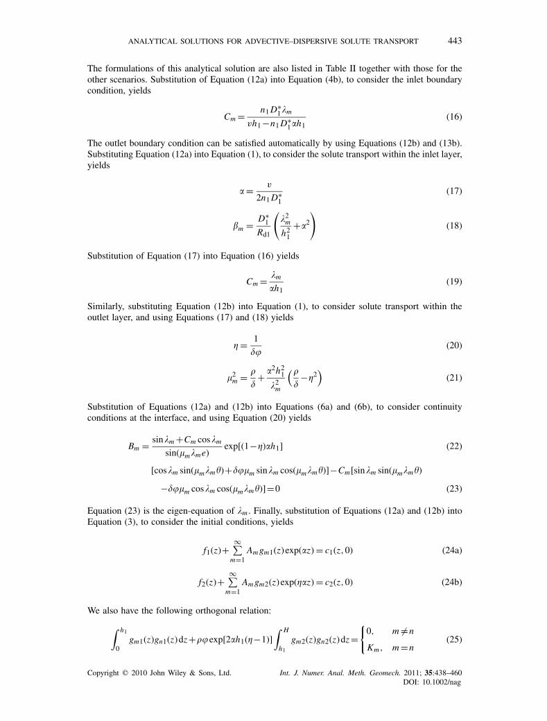
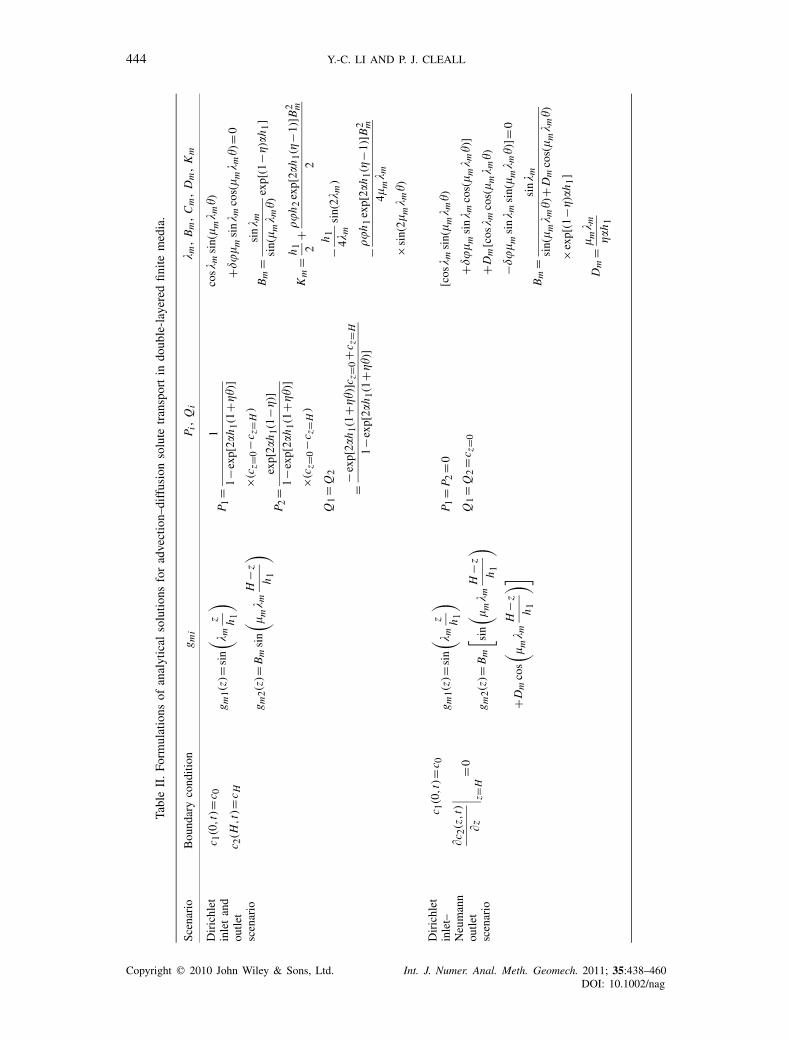
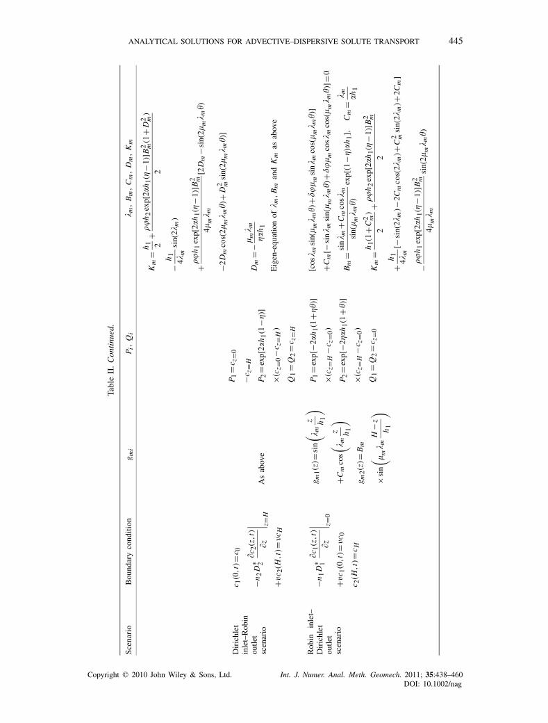
The formulations of this analytical solution are also listed in Table II together with those for theother scenarios. Substitution of Equation (12a) into Equation (4b), to consider the inlet boundarycondition, yields

Cm = n1 D∗1m

vh1 −n1 D∗1�h1

(16)

The outlet boundary condition can be satisfied automatically by using Equations (12b) and (13b).Substituting Equation (12a) into Equation (1), to consider the solute transport within the inlet layer,yields

� = v

2n1 D∗1

(17)

�m = D∗1

Rd1

(2

m

h21

+�2

)(18)

Substitution of Equation (17) into Equation (16) yields

Cm = m

�h1(19)

Similarly, substituting Equation (12b) into Equation (1), to consider solute transport within theoutlet layer, and using Equations (17) and (18) yields

= 1

��(20)

�2m = �

�+ �2h2

1

2m

(�

�−2

)(21)

Substitution of Equations (12a) and (12b) into Equations (6a) and (6b), to consider continuityconditions at the interface, and using Equation (20) yields

Bm = sinm +Cm cosm

sin(�mme)exp[(1−)�h1] (22)

[cosm sin(�mm�)+��m sinm cos(�mm�)]−Cm[sinm sin(�mm�)

−��m cosm cos(�mm�)]=0 (23)

Equation (23) is the eigen-equation of m . Finally, substitution of Equations (12a) and (12b) intoEquation (3), to consider the initial conditions, yields

f1(z)+∞∑

m=1Am gm1(z)exp(�z) = c1(z,0) (24a)

f2(z)+∞∑

m=1Am gm2(z)exp(�z) = c2(z,0) (24b)

We also have the following orthogonal relation:

∫ h1

0gm1(z)gn1(z)dz+��exp[2�h1(−1)]

∫ H

h1

gm2(z)gn2(z)dz ={

0, m �=n

Km, m =n(25)



Tabl

eII

.Fo

rmul

atio

nsof

anal

ytic

also

lutio

nsfo

rad

vect

ion–

diff

usio

nso

lute

tran

spor

tin

doub

le-l

ayer

edfin

item

edia

.

Scen

ario

Bou

ndar

yco

nditi

ong m

iP i

,Q

i m

,B

m,

Cm

,D

m,

Km

Dir

ichl

etin

let

and

outle

tsc

enar

io

c 1(0

,t)=

c 0

c 2(H

,t)=

c Hg m

1(z

)=si

n

( mz h1

)

g m2(z

)=B

msi

n

( � m m

H−

z

h1

)P 1

=1

1−e

xp[2

�h1(1

+�)

]

×(c z

=0−c

z=H

)

P 2=

exp[

2�h

1(1

−)]

1−e

xp[2

�h1(1

+�)

]

×(c z

=0−c

z=H

)

Q1=

Q2

=−

exp[

2�h

1(1

+�)

]cz=

0+c

z=H

1−e

xp[2

�h1(1

+�)

]

cos

msi

n(� m

m�)

+ ��

� msi

n m

cos(

� m m

�)=

0

Bm

=si

n m

sin(

� m m

�)ex

p[(1

− )�

h1]

Km

=h

1 2+

��h

2ex

p[2�

h1(

−1)]

B2 m

2

−h

1

4m

sin(

2m

)

−��

h1

exp[

2�h

1(

−1)]

B2 m

4�m

m

×si

n(2�

m m

�)

Dir

ichl

etin

let–

Neu

man

nou

tlet

scen

ario

c 1(0

,t)=

c 0

�c2(z

,t)

�z

∣ ∣ ∣ ∣ z=H

=0

g m1(z

)=si

n

( mz h1

)

g m2(z

)=B

m

[ sin

( � m m

H−

z

h1

)

+Dm

cos( � m

mH

−z

h1

)]

P 1=

P 2=

0

Q1=

Q2=

c z=0

[cos

msi

n(� m

m�)

+ ��

� msi

n m

cos(

� m m

�)]

+Dm

[cos

mco

s(� m

m�)

− ��

� msi

n m

sin(

� m m

�)]=

0

Bm

=si

n m

sin(

� m m

�)+

Dm

cos(

� m m

�)

×ex

p[(1

− )�

h1]

Dm

=� m

m�

h1



Tabl

eII

.C

onti

nued

.

Scen

ario

Bou

ndar

yco

nditi

ong m

iP i

,Q

i m

,B

m,

Cm

,D

m,

Km

Km

=h

1 2+

��h

2ex

p[2�

h1(

−1)]

B2 m

(1+

D2 m

)

2

−h

1

4m

sin(

2m

)

+��

h1

exp[

2�h

1(

−1)]

B2 m

4�m

m[2

Dm

−sin

(2� m

m�)

−2D

mco

s(2�

m m

�)+

D2 m

sin(

2�m

m�)

]

Dir

ichl

etin

let–

Rob

inou

tlet

scen

ario

c 1(0

,t)=

c 0

−n2

D∗ 2

�c2(z

,t)

�z

∣ ∣ ∣ ∣ z=H

+vc 2

(H,t

)=v

c H

As

abov

e

P 1=

c z=0

−cz=

H

P 2=

exp[

2�h

1(1

−)]

×(c z

=0−c

z=H

)

Q1=

Q2=

c z=H

Dm

=−

� m m

�h

1

Eig

en-e

quat

ion

of m

,B

man

dK

mas

abov

e

Rob

inin

let–

Dir

ichl

etou

tlet

scen

ario

−n1

D∗ 1

�c1(z

,t)

�z

∣ ∣ ∣ ∣ z=0

+vc 1

(0,t

)=v

c 0

c 2(H

,t)=

c H

g m1(z

)=si

n

( mz h1

)

+Cm

cos( m

z h1

)

g m2(z

)=B

m

×si

n

( � m m

H−

z

h1

)

P 1=

exp[

−2�h

1(1

+�)

]

×(c z

=H−c

z=0)

P 2=

exp[

−2�

h1(1

+�)]

×(c z

=H−c

z=0)

Q1=

Q2=

c z=0

[cos

msi

n(� m

m�)

+��

� msi

n m

cos(

� m m

�)]

+Cm

[−si

n m

sin(

� m m

�)+�

�� m

cos

mco

s(� m

m�)

]=0

Bm

=si

n m

+Cm

cos

m

sin(

� m m

�)ex

p[(1

− )�

h1],

Cm

= m �h

1

Km

=h

1(1

+C2 m

)

2+

��h

2ex

p[2�

h1(

−1)]

B2 m

2

+h

1

4m

[−si

n(2

m)−

2Cm

cos(

2m

)+C

2 msi

n(2

m)+

2Cm

]

−��

h1

exp[

2�h

1(

−1)]

B2 m

4�m

msi

n(2�

m m

�)



Tabl

eII

.C

onti

nued

.

Scen

ario

Bou

ndar

yco

nditi

ong m

iP i

,Q

i m

,B

m,

Cm

,D

m,

Km

Rob

inin

let-

Neu

man

nou

tlet

scen

ario

−n1

D∗ 1

�c1(z

,t)

�z

∣ ∣ ∣ ∣ z=0

+vc 1

(0,t

)=v

c 0

�c2(z

,t)

�z

∣ ∣ ∣ ∣ z=H

=0

g m1(z

)=si

n

( mz h1

)

+Cm

cos( m

z h1

)

g m2(z

)=B

m

[ sin

( � m m

H−

z

h1

)

+Dm

cos( � m

mH

−z

h1

)]

P 1=

P 2=

0

Q1=

Q2=

c z=0

[cos

msi

n(� m

m�)

+��

� msi

n m

cos(

� m m

�)]

+Cm

[−si

n m

sin(

� m m

�)+�

�� m

cos

mco

s(� m

m�)

]

+Dm

[cos

mco

s(� m

m�)

−��

� msi

n m

sin(

� m m

�)]

+Cm

Dm

[−si

n m

cos(

� m m

�)

− ��

� mco

sm

sin(

� m m

�)]=

0

Bm

=si

n m

+Cm

cos

m

sin(

� m m

�)+

Dm

cos(

� m m

�)ex

p[(1

− )�

h1],

Cm

= m �h

1,

Dm

=� m

m�

h1

Km

=h

1(1

+C2 m

)

2+

��h

2ex

p[2�

h1(

−1)]

B2 m

(1+

D2 m

)

2

+h

1

4m

[−si

n(2

m)−

2Cm

cos(

2m

)

+C2 m

sin(

2m

)+2C

m]

+��

h1

exp[

2�h

1(

−1)]

B2 m

4�m

m

+[2

Dm

−sin

(2� m

m�)

−2D

mco

s(2�

m m

�)+

D2 m

sin(

2�m

m�)

]

�=

D∗ 2/

D∗ 1,�

=R

d2/

Rd1

,�=

n 2/n 1

,�=

h2/h

1,

H=

h1+h

2,c

1(z

,t)=

f 1(z

)+∑ ∞ m

=1A

mg m

1(z

)exp

(�z−

� mt)

,c2(z

,t)=

f 2(z

)+∑ ∞ m

=1A

mg m

2(z

)exp

(�z

−�m

t),

f 1(z

)=P 1

exp(

2�z)

+Q

1,

f 2(z

)=P 2

exp(

2�z

)+Q

2,

�=

v/(2

n 1D

∗ 1),

� m=

(D∗ 1/

Rd1

)(2 m

/h

2 1+�

2),

=

1/(�

�),

�2 m=

�/�+(

�2h

2 1/2 m

)(�/

�−

2),

Km

=∫ h 1 0

g m1(z

)gm

1(z

)dz+

��ex

p[2�

h1(

−1)]∫ H h

1g m

2(z

)gm

2(z

)dz.



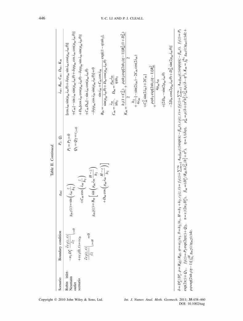
where Km can be written as the following expression for the scenario considered:

Km = h1(1+C2m)

2+ ��h2 exp[2�h1(−1)]B2

m

2

+ h1

4m[−sin(2m)−2Cm cos(2m)+C2

m sin(2m)+2Cm]

−��h1 exp[2�h1(−1)]B2m

4�mmsin(2�mm�) (26)

Using Equations (24)–(26), the following formulation for Am can be obtained:

Am = 1

Km

∫ h1

0gm1(z)

c1(z,0)− f1(z)

exp(�z)dz+ ��exp[2�h1(−1)]

Km

×∫ H

h1

gm2(z)c2(z,0)− f2(z)

exp(�z)dz (27)

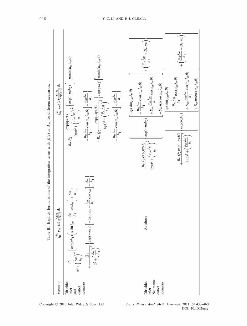
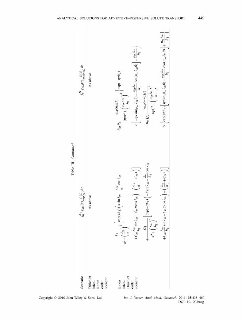
The integration terms of∫ h1

0 gm1(z) f1(z)exp(−�z)dz and∫ H

h1gm2(z) f2(z)exp(−�z)dz in Equa-

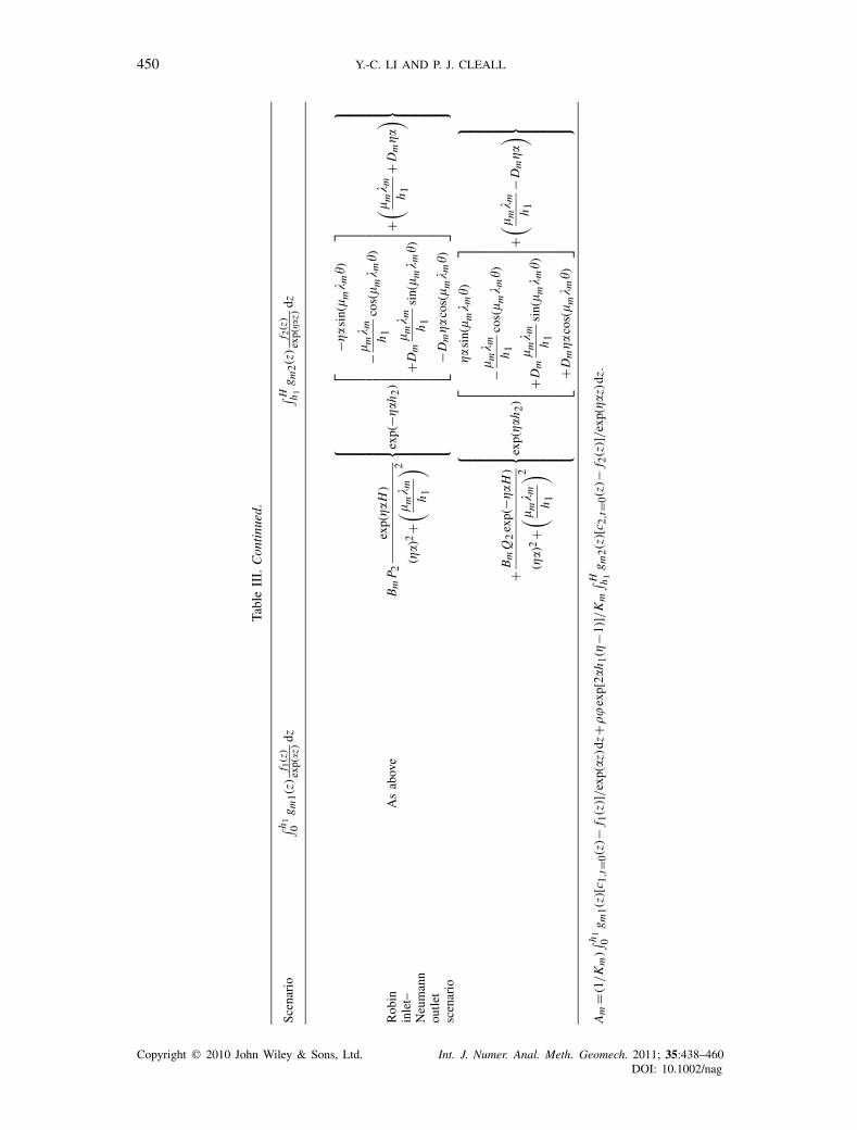
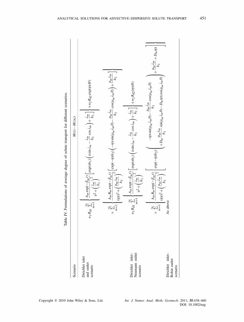
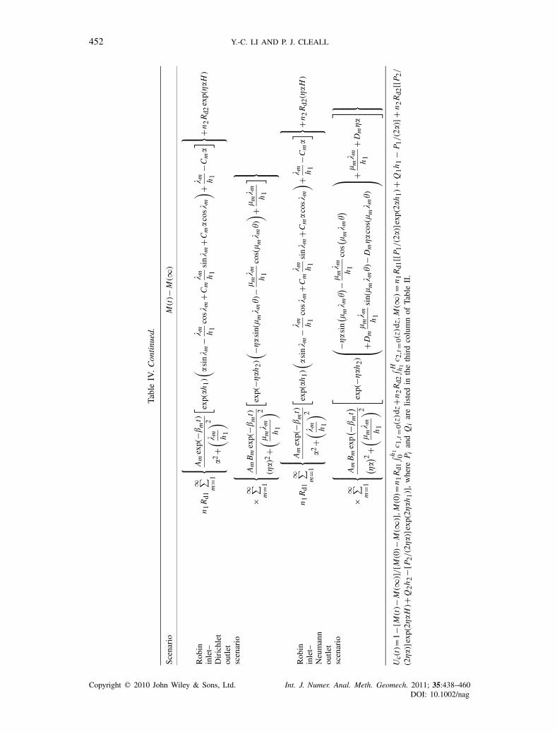
tion (27) can be written explicitly as shown in Table III. The integration terms with the initialconcentration functions in Equation (27) might also be written explicitly if ci (z) has a simpleform, such as a unique function; otherwise, numerical integration techniques [14] can be employedto obtain their integration values. The terms M(∞) and M(t)− M(∞) in the formulation of theaverage degree of solute transport, i.e. Equation (9), for the scenario considered can be obtainedusing Equations (12), (13) and (15) and are shown in Table IV.

Similar analytical solutions for the other four scenarios in Table I are detailed in Table II.The unknown coefficients can be obtained following the procedure presented for the Robin inlet–Dirichlet outlet scenario and can also be found in Table II. The analytical solution for the scenariowith zero flux conditions at both the inlet and outlet boundaries is the same as that for the Robininlet–Neumann outlet scenario except Pi = Qi =0. The eigen-equations of m for these analyticalsolutions can be solved by the ‘sign-count’ method [6, 15].

The outlet boundary condition and continuity conditions at the interface are satisfied by estab-lishing an appropriate term of gmi (z). The infinite series solution might converge slowly forrelatively large values of the column Peclet number [13], PH,i , which can be defined for the i thlayer of the double-layered media considered by

PH,i = vhi

ni D∗i

(28)

Following van Genuchten and Alves [16], the following range of application of the presentedanalytical solutions is suggested:

PH,i<5+40vt

Rdi hi(29)

For the problems having larger PH,i values, approximate solutions, which can be derived via theLaplace transform techniques and the binomial theorem following Leij and van Genuchten [5],may provide satisfactory answers.

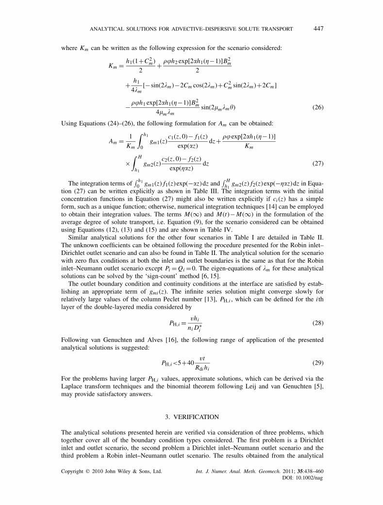
3. VERIFICATION

The analytical solutions presented herein are verified via consideration of three problems, whichtogether cover all of the boundary condition types considered. The first problem is a Dirichletinlet and outlet scenario, the second problem a Dirichlet inlet–Neumann outlet scenario and thethird problem a Robin inlet–Neumann outlet scenario. The results obtained from the analytical



Tabl

eII

I.E

xplic

itfo

rmul

atio

nsof

the

inte

grat

ion

term

sw

ithf i

(z)

inA

mfo

rdi

ffer

ent

scen

ario

s.

Scen

ario

∫ h 1 0g m

1(z

)f 1

(z)

exp(

�z)

dz∫ H h

1g m

2(z

)f 2

(z)

exp(

�z)

dz

Dir

ichl

etin

let

and

outle

tsc

enar

io

P 1

�2+( m h

1

) 2{ exp(

�h1)[ �

sin m

− m h

1co

sm

] + m h

1

}

+Q

1

�2+( m h

1

) 2{ exp(

− �h

1)[ −�

sin m

− m h

1co

sm

] + m h

1

}

Bm

P 2ex

p(�

H)

(�)

2+( � m

m h1

) 2{ exp(

− �h

2)[ −

�si

n(� m

m�)

−� m

m h1

cos(

� m m

�)] +

� m m h1

}

+Bm

Q2

exp(

−�

H)

(�)

2+( � m

m h1

) 2{ exp(

�h

2)[ �

sin(

� m m

�)

−� m

m h1

cos(

� m m

�)] +

� m m h1

}

Dir

ichl

etin

let–

Neu

man

nou

tlet

scen

ario

As

abov

eB

mP 2

exp(

�H

)

(�)

2+( � m

m h1

) 2⎧ ⎪ ⎪ ⎪ ⎪ ⎪ ⎪ ⎪ ⎪ ⎪ ⎨ ⎪ ⎪ ⎪ ⎪ ⎪ ⎪ ⎪ ⎪ ⎪ ⎩exp(

− �h

2)⎡ ⎢ ⎢ ⎢ ⎢ ⎢ ⎢ ⎢ ⎢ ⎢ ⎣−

�si

n(� m

m�)

−� m

m h1

cos(

� m m

�)

+Dm

� m m h1

sin(

� m m

�)

−Dm

�co

s(� m

m�)

⎤ ⎥ ⎥ ⎥ ⎥ ⎥ ⎥ ⎥ ⎥ ⎥ ⎦+( � m m h1

+D

m�)⎫ ⎪ ⎪ ⎪ ⎪ ⎪ ⎪ ⎪ ⎪ ⎪ ⎬ ⎪ ⎪ ⎪ ⎪ ⎪ ⎪ ⎪ ⎪ ⎪ ⎭

+B

mQ

2ex

p(−

�H

)

(�)

2+( � m

m h1

) 2⎧ ⎪ ⎪ ⎪ ⎪ ⎪ ⎪ ⎪ ⎪ ⎪ ⎨ ⎪ ⎪ ⎪ ⎪ ⎪ ⎪ ⎪ ⎪ ⎪ ⎩exp(

�h

2)⎡ ⎢ ⎢ ⎢ ⎢ ⎢ ⎢ ⎢ ⎢ ⎢ ⎣�

sin(

� m m

�)

−� m

m h1

cos(

� m m

�)

+Dm

� m m h1

sin(

� m m

�)

+Dm

�co

s(� m

m�)

⎤ ⎥ ⎥ ⎥ ⎥ ⎥ ⎥ ⎥ ⎥ ⎥ ⎦+( � m m h1

−D

m�)⎫ ⎪ ⎪ ⎪ ⎪ ⎪ ⎪ ⎪ ⎪ ⎪ ⎬ ⎪ ⎪ ⎪ ⎪ ⎪ ⎪ ⎪ ⎪ ⎪ ⎭



Tabl

eII

I.C

onti

nued

.

Scen

ario

∫ h 1 0g m

1(z

)f 1

(z)

exp(

�z)

dz∫ H h

1g m

2(z

)f 2

(z)

exp(

�z)

dz

Dir

ichl

etin

let–

Rob

inou

tlet

scen

ario

As

abov

eA

sab

ove

Rob

inin

let–

Dir

ichl

etou

tlet

scen

ario

P 1

�2+( m h

1

) 2[ exp(

�h1)( �

sin m

− m h

1co

sm

+Cm

m h1

sin m

+Cm

�co

sm

) +( m h1

−Cm

�)]

+Q

1

�2+( m h

1

) 2[ exp(

− �h

1)( −�

sin m

− m h

1co

sm

+Cm

m h1

sin m

−Cm

�co

sm

) +( m h1

+Cm

�)]

Bm

P 2ex

p(�

H)

(�)

2+( � m

m h1

) 2{ exp(

−�h

2)

×[ −

�si

n(� m

m�)

−� m

m h1

cos(

� m m

�)] +

� m m h1

}

+Bm

Q2

exp(

−�

H)

(�)

2+( � m

m h1

) 2

×{ ex

p(�

h2)[ �

sin(

� m m

�)−

� m m h1

cos(

� m m

�)] +

� m m h1

}



Tabl

eII

I.C

onti

nued

.

Scen

ario

∫ h 1 0g m

1(z

)f 1

(z)

exp(

�z)

dz∫ H h

1g m

2(z

)f 2

(z)

exp(

�z)

dz

Rob

inin

let–

Neu

man

nou

tlet

scen

ario

As

abov

eB

mP 2

exp(

�H

)

(�)

2+( � m

m h1

) 2⎧ ⎪ ⎪ ⎪ ⎪ ⎪ ⎪ ⎪ ⎪ ⎪ ⎨ ⎪ ⎪ ⎪ ⎪ ⎪ ⎪ ⎪ ⎪ ⎪ ⎩exp(

− �h

2)⎡ ⎢ ⎢ ⎢ ⎢ ⎢ ⎢ ⎢ ⎢ ⎢ ⎣

− �

sin(

� m m

�)

−� m

m h1

cos(

� m m

�)

+Dm

� m m h1

sin(

� m m

�)

−Dm

�co

s(� m

m�)

⎤ ⎥ ⎥ ⎥ ⎥ ⎥ ⎥ ⎥ ⎥ ⎥ ⎦+( � m m h1

+D

m�)⎫ ⎪ ⎪ ⎪ ⎪ ⎪ ⎪ ⎪ ⎪ ⎪ ⎬ ⎪ ⎪ ⎪ ⎪ ⎪ ⎪ ⎪ ⎪ ⎪ ⎭

+B

mQ

2ex

p(−

�H

)

(�)

2+( � m

m h1

) 2⎧ ⎪ ⎪ ⎪ ⎪ ⎪ ⎪ ⎪ ⎪ ⎪ ⎨ ⎪ ⎪ ⎪ ⎪ ⎪ ⎪ ⎪ ⎪ ⎪ ⎩exp(

�h

2)⎡ ⎢ ⎢ ⎢ ⎢ ⎢ ⎢ ⎢ ⎢ ⎢ ⎣

�si

n(� m

m�)

−� m

m h1

cos(

� m m

�)

+Dm

� m m h1

sin(

� m m

�)

+Dm

�co

s(� m

m�)

⎤ ⎥ ⎥ ⎥ ⎥ ⎥ ⎥ ⎥ ⎥ ⎥ ⎦+( � m m h1

−D

m�)⎫ ⎪ ⎪ ⎪ ⎪ ⎪ ⎪ ⎪ ⎪ ⎪ ⎬ ⎪ ⎪ ⎪ ⎪ ⎪ ⎪ ⎪ ⎪ ⎪ ⎭

Am

=(1

/K

m)∫ h

10

g m1(z

)[c 1

,t=0

(z)−

f 1(z

)]/ex

p(�z

)dz+

��ex

p[2�

h1(

−1)]/

Km∫ H h

1g m

2(z

)[c 2

,t=0

(z)−

f 2(z

)]/ex

p(�

z)dz

.



Tabl

eIV

.Fo

rmul

atio

nsof

aver

age

degr

eeof

solu

tetr

ansp

ort

for

diff

eren

tsc

enar

ios.

Scen

ario

M(t

)−M

(∞)

Dir

ichl

etin

let

and

outle

tsc

enar

ion 1

Rd1

∞ ∑ m=1

⎧ ⎪ ⎪ ⎪ ⎨ ⎪ ⎪ ⎪ ⎩Am

exp(

−�m

t)

�2+( m h

1

) 2[ ex

p(�h

1)( �

sin m

− m h

1co

sm

) + m h

1

]⎫ ⎪ ⎪ ⎪ ⎬ ⎪ ⎪ ⎪ ⎭+n2

Rd2

exp(

�H

)

×∞ ∑ m=1

⎧ ⎪ ⎪ ⎪ ⎨ ⎪ ⎪ ⎪ ⎩Am

Bm

exp(

−�m

t)

(�)

2+( � m

m h1

) 2[ exp(

− �h

2)( −

�si

n(� m

m�)

−� m

m h1

cos(

� m m

�)) +

� m m h1

]⎫ ⎪ ⎪ ⎪ ⎬ ⎪ ⎪ ⎪ ⎭D

iric

hlet

inle

t–N

eum

ann

outle

tsc

enar

io

n 1R

d1∞ ∑ m=1

⎧ ⎪ ⎪ ⎪ ⎨ ⎪ ⎪ ⎪ ⎩Am

exp(

−�m

t)

�2+( m h

1

) 2[ ex

p(�h

1)( �

sin m

− m h

1co

sm

) + m h

1

]⎫ ⎪ ⎪ ⎪ ⎬ ⎪ ⎪ ⎪ ⎭+n2

Rd2

(�

H)

×∞ ∑ m=1

⎧ ⎪ ⎪ ⎪ ⎨ ⎪ ⎪ ⎪ ⎩Am

Bm

exp(

−�m

t)

(�)

2+( � m

m h1

) 2⎡ ⎢ ⎢ ⎢ ⎣exp(

− �h

2)⎛ ⎜ ⎜ ⎜ ⎝

− �

sin(

� m m

�)−

� m m h1

cos(

� m m

�)

+Dm

� m m h1

sin(

� m m

�)−

Dm

�co

s(� m

m�)

⎞ ⎟ ⎟ ⎟ ⎠+� m

m h1

+D

m�

⎤ ⎥ ⎥ ⎥ ⎦⎫ ⎪ ⎪ ⎪ ⎬ ⎪ ⎪ ⎪ ⎭D

iric

hlet

inle

t–R

obin

outle

tsc

enar

io

As

abov

e



Tabl

eIV

.C

onti

nued

.

Scen

ario

M(t

)−M

(∞)

Rob

inin

let–

Dir

ichl

etou

tlet

scen

ario

n 1R

d1∞ ∑ m=1

⎧ ⎪ ⎪ ⎪ ⎨ ⎪ ⎪ ⎪ ⎩Am

exp(

−�m

t)

�2+( m h

1

) 2[ ex

p(�h

1)( �

sin m

− m h

1co

sm

+Cm

m h1

sin m

+Cm

�co

sm

) + m h

1−C

m�]⎫ ⎪ ⎪ ⎪ ⎬ ⎪ ⎪ ⎪ ⎭+n

2R

d2ex

p(�

H)

×∞ ∑ m=1

⎧ ⎪ ⎪ ⎪ ⎨ ⎪ ⎪ ⎪ ⎩Am

Bm

exp(

−�m

t)

(�)

2+( � m

m h1

) 2[ exp(

− �h

2)( −

�si

n(� m

m�)

−� m

m h1

cos(

� m m

�)) +

� m m h1

]⎫ ⎪ ⎪ ⎪ ⎬ ⎪ ⎪ ⎪ ⎭R

obin

inle

t–N

eum

ann

outle

tsc

enar

io

n 1R

d1∞ ∑ m=1

⎧ ⎪ ⎪ ⎪ ⎨ ⎪ ⎪ ⎪ ⎩Am

exp(

−�m

t)

�2+( m h

1

) 2[ ex

p(�h

1)( �

sin m

− m h

1co

sm

+Cm

m h1

sin m

+Cm

�co

sm

) + m h

1−C

m�]⎫ ⎪ ⎪ ⎪ ⎬ ⎪ ⎪ ⎪ ⎭+n

2R

d2(

�H

)

×∞ ∑ m=1

⎧ ⎪ ⎪ ⎪ ⎪ ⎨ ⎪ ⎪ ⎪ ⎪ ⎩Am

Bm

exp( −�

mt)

( �) 2 +( � m

m h1

) 2⎡ ⎢ ⎢ ⎢ ⎢ ⎣exp(

− �h

2)⎛ ⎜ ⎜ ⎜ ⎜ ⎝−

�si

n( � m

m�) −

� m m h1

cos( � m

m�)

+Dm

� m m h1

sin(

� m m

�)−

Dm

�co

s(� m

m�)

⎞ ⎟ ⎟ ⎟ ⎟ ⎠+� m

m h1

+D

m�

⎤ ⎥ ⎥ ⎥ ⎥ ⎦⎫ ⎪ ⎪ ⎪ ⎪ ⎬ ⎪ ⎪ ⎪ ⎪ ⎭U

c(t)

=1−[

M(t

)−M

(∞)]

/[M

(0)−

M(∞

)],

M(0

)=n 1

Rd1∫ h 1 0

c 1,t

=0(z

)dz+

n 2R

d2∫ H h

1c 2

,t=

0(z

)dz,

M(∞

)=n 1

Rd1

[[P 1

/(2

�)]e

xp(2

�h1)+

Q1h

1−

P 1/(2

�)]+

n 2R

d2[[

P 2/

(2�

)]ex

p(2

�H

)+Q

2h

2−[

P 2/(2

�)]

exp(

2�h

1)]

,w

here

P ian

dQ

iar

elis

ted

inth

eth

ird

colu

mn

ofTa

ble

II.



solutions are compared for the first two problems with a numerical solution using the finite elementmethod [17, 18] and for the third problem with an alternative analytical solution using a Laplacetransformation approach for solute transport in a two-layer porous media [5].

For the first problem, the two layers are defined to initially have a zero solute concentration.The solute concentration is assumed to be fixed at a value of c0 at the inlet boundary and fixed atzero at the outlet boundary, which is often considered as appropriate if an aquifer is present belowthe outlet boundary. According to the boundary conditions considered, the analytical solution forDirichlet inlet and outlet scenario presented in Table II is applied to analyze this problem. Thesoil and transport properties for the inlet layer are assumed as: D∗

1 =5×10−10 m2/s, Rd1 =2.0 andn1 =0.4. A number of analyses have been undertaken with varying values of �, �, �, �, H and v

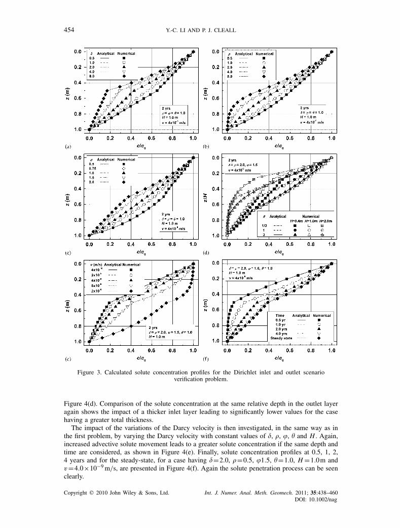
to illustrate the uniqueness of the solutions and the results of these analyses are presented below.Firstly, three series of analyses are performed, all with �=1, H =1.0m and v=4.0×10−9 m/s,

where one of �, �, � is varied with others remaining at unity. This allows the impact of the variationsof �, � and � to be investigated. Calculated solute concentration profiles at 2 years for these threeseries of analyses are shown in Figures 3(a)–(c), respectively, together with those obtained bythe numerical approach. The impact of the variation of the effective diffusion coefficients and theporosities between the two layers can be clearly seen with a distinct change in the concentrationgradient at the interface from Figures 3(a) and 3(c). This is due to the fact that the interfaceboundary conditions applied are dependent on the effective diffusion coefficients and the porosities,as shown in Equation (7). Such concentration gradient changes cannot be found in Figure 3(b) asthe interface boundary conditions are independent of the retardation factors.

A series of cases with �=2.0, �=0.5, �=1.5, v=4.0×10−9 m/s, varying total thicknesses(0.4, 1.0 and 2.0 m) and different ratios of thickness for the inlet and outlet layers (i.e. �= 1

3 ,1,3)are then considered. The calculated results at 2 years are shown in Figure 3(d). Comparison of thesolute concentration at the same relative depth in the outlet layer shows the impact of a thickerinlet layer leading to significantly lower values for the case having a greater total thickness. Thisis due to the increased time required to penetrate through a thicker inlet layer.

The impact of variations in Darcy velocity is then investigated by a series of cases with �=2.0,�=0.5, �=1.5, �=1.0, H =1.0m and varying Darcy velocity (4.0×10−10 m/s, 2.0×10−9 m/s,4.0×10−9 m/s, 8.0×10−9 m/s and 2.0×10−8 m/s). The advective effect of pore-water movementleads to a greater solute concentration for the case with a higher Darcy velocity if the same depthand time are considered, as shown in Figure 3(e). Finally, solute concentration profiles at 0.5, 1,2, 4 years and for the steady-state, for a case having �=2.0, �=0.5, �=1.5, �=1.0, H =1.0mand v=4.0×10−9 m/s, are presented in Figure 3(f) where the solute penetration process can beseen clearly.

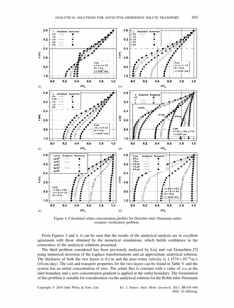
The second problem considers two layers that are defined to initially have a zero solute concen-tration. In this case, it is assumed that the solute concentration is fixed at the inlet boundaryand the solute concentration gradient is held at zero at the outlet boundary, which matches theDirichlet inlet–Neumann outlet scenario presented in Table I. The soil and transport properties forthe inlet layer for the first problem are also adopted here. Again a series of three analyses areperformed, all with �=1, H =1.0m and v=4.0×10−9 m/s, where one of �, �, � is varied withothers remaining at unity. The calculated results obtained by the analytical and numerical solutionsare shown in Figures 4(a)–(c). The impact of the variation in effective diffusion coefficients andporosities between the two layers is again clearly seen with a distinct change in the concentrationgradient at the interface. The impact of variation in effective diffusion coefficients (Figure 4(a)) isalso more complex than for variations in porosities and retardation factors, with a relative decreasein the lower layer effective diffusion coefficient leading to a relatively higher concentration in theupper regions and a relatively lower concentration in the lower regions. This is a result of theimpact of the lower boundary condition on the system increasing as the lower layers effectivediffusion coefficient increases.

As in the first problem a series of cases with �=2.0, �=0.5, �=1.5, v=4.0×10−9 m/s,varying total thicknesses (0.4, 1.0 and 2.0 m) and different ratios of thickness for the inlet andoutlet layers (i.e. �= 1

3 ,1,3) are then considered. The calculated results at 2 years are shown in



Figure 3. Calculated solute concentration profiles for the Dirichlet inlet and outlet scenarioverification problem.

Figure 4(d). Comparison of the solute concentration at the same relative depth in the outlet layeragain shows the impact of a thicker inlet layer leading to significantly lower values for the casehaving a greater total thickness.

The impact of the variations of the Darcy velocity is then investigated, in the same way as inthe first problem, by varying the Darcy velocity with constant values of �, �, �, � and H . Again,increased advective solute movement leads to a greater solute concentration if the same depth andtime are considered, as shown in Figure 4(e). Finally, solute concentration profiles at 0.5, 1, 2,4 years and for the steady-state, for a case having �=2.0, �=0.5, �1.5, �=1.0, H =1.0m andv=4.0×10−9 m/s, are presented in Figure 4(f). Again the solute penetration process can be seenclearly.



Figure 4. Calculated solute concentration profiles for Dirichlet inlet–Neumann outletscenario verification problem.

From Figures 3 and 4, it can be seen that the results of the analytical analysis are in excellentagreement with those obtained by the numerical simulations, which builds confidence in thecorrectness of the analytical solutions presented.

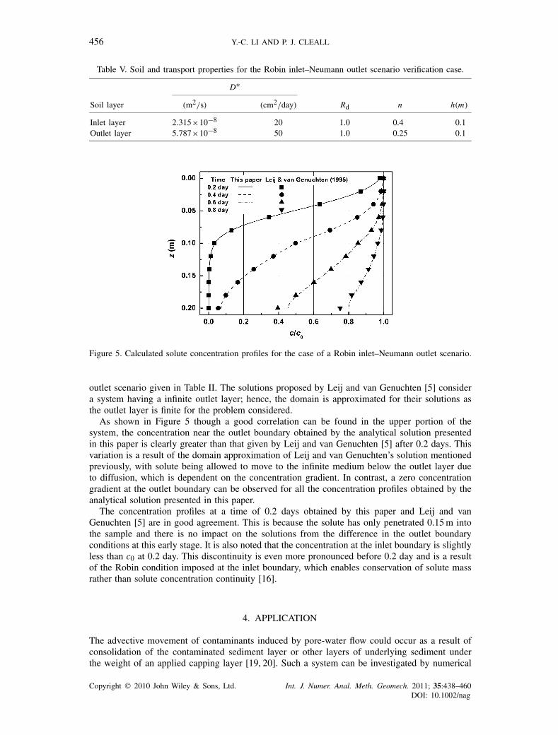
The third problem considered has been previously analyzed by Leij and van Genuchten [5]using numerical inversion of the Laplace transformations and an approximate analytical solution.The thickness of both the two layers is 0.1 m and the pore-water velocity is 1.1574×10−6 m/s(10 cm/day). The soil and transport properties for the two layers can be found in Table V and thesystem has an initial concentration of zero. The solute flux is constant with a value of vc0 at theinlet boundary and a zero concentration gradient is applied at the outlet boundary. The formulationof this problem is suitable for consideration via the analytical solution for the Robin inlet–Neumann



Table V. Soil and transport properties for the Robin inlet–Neumann outlet scenario verification case.

D∗

Soil layer (m2/s) (cm2/day) Rd n h(m)

Inlet layer 2.315×10−8 20 1.0 0.4 0.1Outlet layer 5.787×10−8 50 1.0 0.25 0.1

Figure 5. Calculated solute concentration profiles for the case of a Robin inlet–Neumann outlet scenario.

outlet scenario given in Table II. The solutions proposed by Leij and van Genuchten [5] considera system having a infinite outlet layer; hence, the domain is approximated for their solutions asthe outlet layer is finite for the problem considered.

As shown in Figure 5 though a good correlation can be found in the upper portion of thesystem, the concentration near the outlet boundary obtained by the analytical solution presentedin this paper is clearly greater than that given by Leij and van Genuchten [5] after 0.2 days. Thisvariation is a result of the domain approximation of Leij and van Genuchten’s solution mentionedpreviously, with solute being allowed to move to the infinite medium below the outlet layer dueto diffusion, which is dependent on the concentration gradient. In contrast, a zero concentrationgradient at the outlet boundary can be observed for all the concentration profiles obtained by theanalytical solution presented in this paper.

The concentration profiles at a time of 0.2 days obtained by this paper and Leij and vanGenuchten [5] are in good agreement. This is because the solute has only penetrated 0.15 m intothe sample and there is no impact on the solutions from the difference in the outlet boundaryconditions at this early stage. It is also noted that the concentration at the inlet boundary is slightlyless than c0 at 0.2 day. This discontinuity is even more pronounced before 0.2 day and is a resultof the Robin condition imposed at the inlet boundary, which enables conservation of solute massrather than solute concentration continuity [16].

4. APPLICATION

The advective movement of contaminants induced by pore-water flow could occur as a result ofconsolidation of the contaminated sediment layer or other layers of underlying sediment underthe weight of an applied capping layer [19, 20]. Such a system can be investigated by numerical



Table VI. Soil and transport properties for capping layer and contaminated sediment.

Soil layer D∗(m2/s) Rd n h (m)

Capping layer 9.8×10−10 1.0 0.38 0.6Sediment 9.4×10−10 2.0 0.45 0.4

approaches that consider some aspects of coupling consolidation and contaminant transport [21, 22].However, such approaches are relatively complex and often beyond practical implementation.

In this section, the analytical solution for the Robin inlet–Dirichlet outlet scenario presentedin this paper is applied to investigate such advective effects on contaminant penetration in acapped contaminated sediment system. A 0.4 m thick sediment is considered to be contaminatedby trichloropropane (TCP) and covered by a 0.6 m thick balsam sand capping layer to impedethe TCP from directly dispersing into an overlying surface water body. The soil and transportproperties for these two layers are as defined by Thoma et al. [23] and can be found in Table VI.The retardation factor of the sediment layer is 2.0 and TCP is assumed not to adsorb onto thebalsam sand. An initial concentration of TCP of 150mg/L is taken for the contaminated sedimentand zero for the capping layer.

During primary consolidation [24], the compression of the underlying sediment layers has arelatively high rate and a great amount of pore-water is extruded from these layers. Consequently,contaminant transport within the capping contaminated system during the primary consolidationis controlled simultaneously by advection and diffusion. Here, it is assumed that the pore-waterpenetrates the capping layer and contaminated layer with a constant velocity during the primaryconsolidation of a soft underlying sediment layer. The value of the pore-water velocity can becalculated based on the duration and the volume of pore-water squeezed in the primary consoli-dation that can be obtained by traditional consolidation analysis methods, i.e. Terzaghi’s theory ofconsolidation [11].

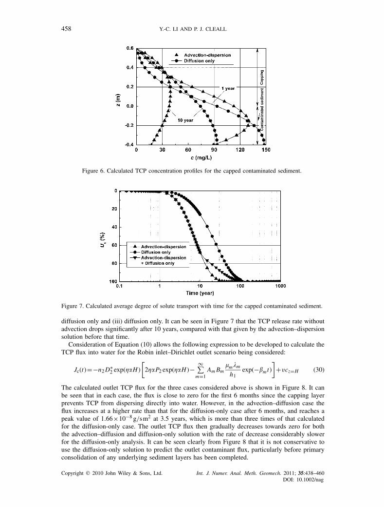
For the problem considered, it is assumed that the primary consolidation of the underlyingsediment layer is complete 10 years after the capping layer is placed and the associated pore-watervelocity is 1.5×10−9 m/s. A zero flux condition is assumed at the inlet boundary and a zeroconcentration at the outlet boundary to model the washing effect of the surface water. The presentedanalytical solution for the Robin inlet–Dirichlet outlet scenario in Table II is used to calculatethe TCP concentration profiles at elapsed times of 1 and 10 years, as illustrated in Figure 6.In addition, the results of a diffusion only analysis (considered here by setting the pore-watervelocity to a value approaching zero in the Robin inlet–Dirichlet outlet scenario analytical solution)are also shown in Figure 6. It can be observed clearly from the advection–dispersion concentrationprofiles that TCP is carried upward by the pore-water flow compared with when only diffusionis considered. Also the advection–dispersion concentration profiles have a peak value within thelayers rather than, as for the diffusion-only solution, at the bottom.

The acceleration of TCP release into the fresh water above the top boundary due to considerationof advection can be clearly observed in Figure 7, where the calculated average degree of solutetransport against time is shown. At the end of the primary consolidation, which is after an elapsedtime of 10 years, according to the advection–dispersion solution nearly 70% of TCP has dispersedinto water whereas only 26% has dispersed in the diffusion-only case.

During the time following primary consolidation, that is during secondary consolidation [24],consolidation occurs at a very slow rate and a relatively small amount of pore-water is extrudedout of the system. Contaminant transport in the capping sediment system is then controlled bydiffusion and the pore-water velocity can be assumed to be small. To consider this change in thepore-water velocity field the Robin inlet–Dirichlet outlet scenario analytical solution with the pore-water velocity set to a value approaching zero and the initial concentration distribution followingthat obtained by the advection–dispersion analytical solution at 10 years can be used. The results ofanalyses considering the system after 10 years are also shown in Figure 7 with three sets of resultsshown (i) advection–dispersion with a constant pore-water velocity throughout (from 0 to 1000years), (ii) advection–dispersion with a constant pore-water velocity for the first 10 years and then



Figure 6. Calculated TCP concentration profiles for the capped contaminated sediment.

Figure 7. Calculated average degree of solute transport with time for the capped contaminated sediment.

diffusion only and (iii) diffusion only. It can be seen in Figure 7 that the TCP release rate withoutadvection drops significantly after 10 years, compared with that given by the advection–dispersionsolution before that time.

Consideration of Equation (10) allows the following expression to be developed to calculate theTCP flux into water for the Robin inlet–Dirichlet outlet scenario being considered:

Jc(t)=−n2 D∗2 exp(�H )

[2�P2 exp(�H )−

∞∑m=1

Am Bm�mm

h1exp(−�mt)

]+vcz=H (30)

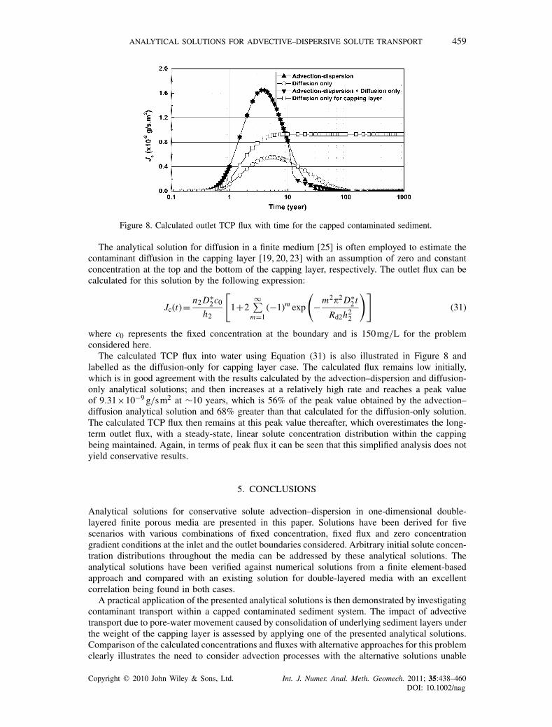
The calculated outlet TCP flux for the three cases considered above is shown in Figure 8. It canbe seen that in each case, the flux is close to zero for the first 6 months since the capping layerprevents TCP from dispersing directly into water. However, in the advection–diffusion case theflux increases at a higher rate than that for the diffusion-only case after 6 months, and reaches apeak value of 1.66×10−8 g/sm2 at 3.5 years, which is more than three times of that calculatedfor the diffusion-only case. The outlet TCP flux then gradually decreases towards zero for boththe advection–diffusion and diffusion-only solution with the rate of decrease considerably slowerfor the diffusion-only analysis. It can be seen clearly from Figure 8 that it is not conservative touse the diffusion-only solution to predict the outlet contaminant flux, particularly before primaryconsolidation of any underlying sediment layers has been completed.



Figure 8. Calculated outlet TCP flux with time for the capped contaminated sediment.

The analytical solution for diffusion in a finite medium [25] is often employed to estimate thecontaminant diffusion in the capping layer [19, 20, 23] with an assumption of zero and constantconcentration at the top and the bottom of the capping layer, respectively. The outlet flux can becalculated for this solution by the following expression:

Jc(t)= n2 D∗2c0

h2

[1+2

∞∑m=1

(−1)m exp

(−m2�2 D∗

2 t

Rd2h22

)](31)

where c0 represents the fixed concentration at the boundary and is 150mg/L for the problemconsidered here.

The calculated TCP flux into water using Equation (31) is also illustrated in Figure 8 andlabelled as the diffusion-only for capping layer case. The calculated flux remains low initially,which is in good agreement with the results calculated by the advection–dispersion and diffusion-only analytical solutions; and then increases at a relatively high rate and reaches a peak valueof 9.31×10−9 g/sm2 at ∼10 years, which is 56% of the peak value obtained by the advection–diffusion analytical solution and 68% greater than that calculated for the diffusion-only solution.The calculated TCP flux then remains at this peak value thereafter, which overestimates the long-term outlet flux, with a steady-state, linear solute concentration distribution within the cappingbeing maintained. Again, in terms of peak flux it can be seen that this simplified analysis does notyield conservative results.

5. CONCLUSIONS

Analytical solutions for conservative solute advection–dispersion in one-dimensional double-layered finite porous media are presented in this paper. Solutions have been derived for fivescenarios with various combinations of fixed concentration, fixed flux and zero concentrationgradient conditions at the inlet and the outlet boundaries considered. Arbitrary initial solute concen-tration distributions throughout the media can be addressed by these analytical solutions. Theanalytical solutions have been verified against numerical solutions from a finite element-basedapproach and compared with an existing solution for double-layered media with an excellentcorrelation being found in both cases.

A practical application of the presented analytical solutions is then demonstrated by investigatingcontaminant transport within a capped contaminated sediment system. The impact of advectivetransport due to pore-water movement caused by consolidation of underlying sediment layers underthe weight of the capping layer is assessed by applying one of the presented analytical solutions.Comparison of the calculated concentrations and fluxes with alternative approaches for this problemclearly illustrates the need to consider advection processes with the alternative solutions unable



to yield conservative results. Also, consideration of the different features of contaminant transportdue to varying pore-water velocity fields in primary consolidation and secondary consolidationstages is achieved via the use of non-uniform initial concentration distributions within the proposedanalytical solutions.

ACKNOWLEDGEMENTS

The work presented in this paper was funded by the Engineering and Physical Sciences Research Council,U.K. via project no. EP/C532651/2. This support is greatly appreciated.

REFERENCES

1. Rowe RK, Quigley RM, Brachman RWI, Booker JR. Barrier Systems for Waste Disposal Facilities. Taylor &Francis: Oxford, U.K., 2004.

2. Alniami ANS, Rushton KR. Dispersion in stratified porous media: analytical solutions. Water Resources Research1979; 15(5):1044–1048.

3. Shamir UY, Harleman DRE. Dispersion in layered porous media. Proceedings of ASCE, Journal of the HydraulicsDivision 1967; 93(HY5):237–260.

4. Leij FJ, Dane JH, van Genuchten MT. Mathematical analysis of one-dimensional solute transport in a layeredsoil profile. Soil Science Society of America Journal 1991; 55(4):944–953.

5. Leij FJ, van Genuchten MT. Approximate analytical solutions for solute transport in two-layer porous-media.Transport in Porous Media 1995; 18(1):65–85.

6. Liu C, Ball WP, Ellis JH. An analytical solution to the one-dimensional solute advection-dispersion equation inmulti-layer porous media. Transport in Porous Media 1998; 30(1):25–43.

7. Freeze RA, Cherry JA. Groundwater Modelling Groundwater Flow and Pollution (Theory and Applications ofTransport in Porous Media). D. Reidel Publishing Company: Dordrecht, Holland, 1987.

8. Bear J, Verruijt A. Modelling Groundwater Flow and Pollution (Theory and Application of Transport in PorousMedia). D. Reidel Publishing Company: Dordrecht, Holland, 1987.

9. Eriksson K, Estep D, Hansbo P, Johnson C. Computational Differential Equations. Cambridge University Press:Cambridge, New York, 1996.

10. Shackelford CD, Lee JM. Analyzing diffusion by analogy with consolidation. Journal of Geotechnical andGeoenvironmental Engineering (ASCE) 2005; 131(11):1345–1359.

11. Terzaghi K. Theoretical Soil Mechanics. Wiley: New York, 1943.12. Lee PKK, Xie KH, Cheung YK. A study on one-dimensional consolidation of layered systems. International

Journal for Numerical and Analytical Methods in Geomechanics 1992; 16(11):815–831.13. Xie KH. Theory of one dimensional consolidation of double-layered ground and its applications. Chinese Journal

of Geotechnical Engineering 1994; 16(5):26–38 (in Chinese).14. Chapra SC, Canale RP. Numerical Methods for Engineers (5th edn). McGraw-Hill Higher Education: Boston,

MA, 2006.15. Mikhailov MD, Ozisik MN, Vulchanov NL. Diffusion in composite layers with automatic solution of the

eigenvalue problem. International Journal of Heat and Mass Transfer 1983; 26(8):1131–1141.16. van Genuchten MT, Alves WJ. Analytical solutions of the one-dimensional convective–dispersive solute transport

equation. Technical Bulletin No. 1661, 1982.17. Cleall PJ, Seetharam SC, Thomas HR. Inclusion of some aspects of chemical behavior of unsaturated soil in

thermo/hydro/chemical/mechanical models. I: model development. Journal of Engineering Mechanics (ASCE)2007; 133(3):338–347.

18. Seetharam SC, Thomas HR, Cleall PJ. Coupled thermo/hydro/chemical/mechanical model for unsaturated soils—numerical algorithm. International Journal for Numerical Methods in Engineering 2007; 70(12):1480–1511.

19. Palermo MR, Clausner JE, Rollings MP, Williams GL, Myers TE, Fredette TJ, Randall RE. Guidance forsubaqueous dredged material capping. Technical Report DOER-1, U.S. Army Corps of Engineers, 1998.

20. Palermo MR, Maynord S, Miller J, Reible DD. Guidance for in-situ subaqueous capping of contaminatedsediments. EPA 905-B96–004, Great Lakes National Program Office, 1998.

21. Arega F, Hayter E. Coupled consolidation and contaminant transport model for simulating migration ofcontaminants through the sediment and a cap. Applied Mathematical Modelling 2008; 32(11):2413–2428.

22. Alshawabkeh AN, Rahbar N, Sheahan T. A model for contaminant mass flux in capped sediment underconsolidation. Journal of Contaminant Hydrology 2005; 78(3):147–165.

23. Thoma GJ, Reible DD, Valsaraj KT, Thibodeaux LJ. Efficiency of capping contaminated sediments in-situ.2. Mathematics of diffusion adsorption in the capping layer. Environmental Science and Technology 1993;27(12):2412–2419.

24. Terzaghi K, Peck RB, Mesri G. Soil Mechanics in Engineering Practice (3rd edn). Wiley: New York, NY, 1996.25. Carslaw HS, Jaeger JC. Conduction of Heat in Solids (2nd edn). Oxford University Press: Oxford, 1959.


Documents

Analytical solutions for advective–dispersive solute transport in double-layered finite porous media