ANALYTIC METHODS FOR DIOPHANTINE

PROBLEMS

by

Craig Valere Spencer

A dissertation submitted in partial fulfillmentof the requirements for the degree of

Doctor of Philosophy(Mathematics)

in The University of Michigan2008

Doctoral Committee:

Professor Trevor D. Wooley, University of Bristol, Co-ChairEmeritus Professor Donald J. Lewis, Co-ChairProfessor Jeffrey C. LagariasAssistant Professor Vilma M. MesaAssistant Professor Djordje Milicevic

c© Craig Valere Spencer 2008All Rights Reserved

dedicated to Verna Kisling, Marie Spencer, and the memory of Lyle Kisling and Eldon Spencer

ii

ACKNOWLEDGEMENTS

I would like to thank Trevor Wooley for his advice, help, funding, and patience.

Without his guidance, this thesis would not have been possible, and I would have

probably left Michigan after my second year. I consider myself very fortunate to

have been able to learn how to use the circle method and pursue math research from

Professor Wooley.

I would also like to thank Donald Lewis for stepping in during my last year of

graduate school as my advisor. He provided me we wonderful guidance and support

as I wrote this thesis and applied for jobs.

The material in Chapters III and IV of this thesis were written with Yu-Ru Liu.

I would like to thank Professor Liu for working with me, giving me advice about

research and jobs, and financing a visit to the University of Waterloo.

I would also like to thank all of my math instructors from the University of

Wisconsin-Stout, the USA/Canada Mathcamp, Carleton College, and the University

of Michigan. In particular, I have benefited greatly by studying under Jinho Baik,

Brian Conrad, Stephen DeBacker, Tina Garrett, Jerome William Hoffman, Mark

Krusemeyer, Jeffrey Lagarias, Djordje Milicevic, Hugh Montgomery, David Romano,

and Kannan Soundararajan. In addition, discussions at conferences with Andrew

Granville, Roger Heath-Brown, Henryk Iwaniec, Scott Parsell, Emmanuel Peyre,

and Lynne Walling have helped me select directions for my research. I am also

very grateful to Jeffrey Lagarias, Donald Lewis, Vilma Mesa, Djordje Milicevic, and

iii

Trevor Wooley for serving on my committee. I would like to thank James Hirschfeld

for providing a reference to [19] and Michael Lipnowski for finding an error in the

original proof of Theorem 4.1.

I have been fortunate to have the encouragement of very understanding friends

and family members. Dave Allen, Dave Anderson, Matt Bush, Suzy Dixon, Hualong

Feng, Jasun Gong, Wendy Grus, Mark Iwen, Kelly Kinser, Ryan Kinser, Joel Lepak,

Mike Lieberman, John Mackay, Jared Maruskin, Yogesh More, Kamilah Neighbors,

Andrew Ostergaard, Feng Rong, Sourya Shrestha, Charlotte Spencer, James Spencer,

Ryan Spencer, Suzanne Spencer, Ahmed Teleb, and Diane Vavrichek have put up

with my complaining and helped cheer me up when I have been stuck on problems. I

would also like to thank Jonathan Bober, Peng Gao, Leo Goldmakher, Hester Graves,

Rizwan Khan, Greg McNulty, Matthew Smith, and Ben Weiss for creating an active

learning environment at the University of Michigan for analytic number theory.

Lastly, I would like to thank my best friend, Stacey Doan. She has always been

there for me, and I cannot imagine my life without her.

iv

TABLE OF CONTENTS

DEDICATION . . . . . . . . . . . . . . . . . . . . . . . . . . . . . . . . . . . . . . . . . . ii

ACKNOWLEDGEMENTS . . . . . . . . . . . . . . . . . . . . . . . . . . . . . . . . . . iii

CHAPTER

I. Introduction . . . . . . . . . . . . . . . . . . . . . . . . . . . . . . . . . . . . . . . 1

1.1 Background . . . . . . . . . . . . . . . . . . . . . . . . . . . . . . . . . . . . 11.2 Notation . . . . . . . . . . . . . . . . . . . . . . . . . . . . . . . . . . . . . . 21.3 Diophantine Inequalities . . . . . . . . . . . . . . . . . . . . . . . . . . . . . 2

1.3.1 Diagonal Diophantine Inequalities in Function Fields . . . . . . . . 31.3.2 Diophantine Inequalities and Quasi-Algebraically Closed Fields . . 6

1.4 Additive Combinatorics . . . . . . . . . . . . . . . . . . . . . . . . . . . . . . 71.4.1 A Generalization of Roth’s Theorem in Function Fields . . . . . . . 81.4.2 A Generalization of Roth’s Theorem in Finite Abelian Groups . . . 10

1.5 The Manin Conjecture . . . . . . . . . . . . . . . . . . . . . . . . . . . . . . 12

II. Diophantine Inequalities in Function Fields . . . . . . . . . . . . . . . . . . . 14

2.1 Overview . . . . . . . . . . . . . . . . . . . . . . . . . . . . . . . . . . . . . . 142.2 The Davenport-Heilbronn Method for Function Fields . . . . . . . . . . . . . 162.3 A Weyl-Type Estimate . . . . . . . . . . . . . . . . . . . . . . . . . . . . . . 192.4 The Minor Arc . . . . . . . . . . . . . . . . . . . . . . . . . . . . . . . . . . . 242.5 The Major Arc . . . . . . . . . . . . . . . . . . . . . . . . . . . . . . . . . . . 262.6 The Solvability of λ1z

k1

+ · · · + λszks = 0 in K∞ . . . . . . . . . . . . . . . . 30

III. A Generalization of Roth’s Theorem in Function Fields . . . . . . . . . . . 32

3.1 Overview . . . . . . . . . . . . . . . . . . . . . . . . . . . . . . . . . . . . . . 323.2 Proof of Theorem 3.1 . . . . . . . . . . . . . . . . . . . . . . . . . . . . . . . 33

IV. A Generalization of Roth’s Theorem in Finite Abelian Groups . . . . . . . 39

4.1 Overview . . . . . . . . . . . . . . . . . . . . . . . . . . . . . . . . . . . . . . 394.2 Proof of Theorem 4.1 . . . . . . . . . . . . . . . . . . . . . . . . . . . . . . . 404.3 Proof of Corollary 4.2 . . . . . . . . . . . . . . . . . . . . . . . . . . . . . . . 47

V. The Manin Conjecture for x0y0 + · · · + xsys = 0 . . . . . . . . . . . . . . . . . . 49

5.1 Overview . . . . . . . . . . . . . . . . . . . . . . . . . . . . . . . . . . . . . . 495.2 The Minor Arcs . . . . . . . . . . . . . . . . . . . . . . . . . . . . . . . . . . 525.3 The Major Arcs . . . . . . . . . . . . . . . . . . . . . . . . . . . . . . . . . . 565.4 The Proof of Theorem 5.1 . . . . . . . . . . . . . . . . . . . . . . . . . . . . 65

v

APPENDIX . . . . . . . . . . . . . . . . . . . . . . . . . . . . . . . . . . . . . . . . . . . 70

BIBLIOGRAPHY . . . . . . . . . . . . . . . . . . . . . . . . . . . . . . . . . . . . . . . . 73

vi

CHAPTER I

Introduction

1.1 Background

A main theme in mathematics is the study of integer solutions to equations and

inequalities. These questions are called Diophantine problems in honor of Diophan-

tus of Alexandria’s contributions to the subject in the third century. The study of

such topics as the Fermat equation xn + yn = zn have spanned centuries, beginning

with the study of Pythagorean triples and concluding with the recent work of Taylor

and Wiles (see [41] and [46]). Once thought of as strictly an area of pure mathemat-

ics, Diophantine problems currently lie at the very center of applied fields such as

cryptography and coding theory.

One of the main tools for counting integer solutions to equations and inequalities is

the circle method. Stemming from work of Hardy and Littlewood in the 1920’s (see

[16]), the circle method serves as an interface between Diophantine problems and

harmonic analysis. Namely, detector functions from Fourier analysis can be used

to count integer solutions to Diophantine equations and inequalities. This thesis

explores various themes in number theory through the use of the circle method.

It should be noted that Chapters III and IV cover work completed with Yu-Ru

Liu. Furthermore, the material in Chapters II, III, IV, and V include work from [37],

1

2

[26], [25], and [36], respectively.

1.2 Notation

Although some notation changes from chapter to chapter, we now fix certain

notation which is used throughout the whole thesis. Let f(x) and g(x) be real-

valued functions of x, and suppose that g(x) only takes on positive values. If there

exists a constant c > 0 such that |f(x)| ≤ cg(x) for all x, we write f(x) ≪ g(x)

or f(x) = O(g(x)). If limx→∞ f(x)/g(x) = 0, we say that f(x) = o(g(x)

). If

limx→∞ f(x)/g(x) approaches a positive constant, then f(x) ∼ g(x). If f(x) is a

positive-valued function and f(x) ≪ g(x), we may also write g(x) ≫ f(x). Lastly,

whenever ǫ appears in a statement, we are asserting that the statement holds for any

ǫ > 0.

1.3 Diophantine Inequalities

In 1929, Oppenheim (see [31]) stated a weaker version of the following conjecture,

which became known as the Oppenheim conjecture.

Conjecture 1.1. Let Q(x1, . . . , xn) be a nondegenerate quadratic form. Suppose

that n ≥ 3, that Q(x) takes on both positive and negative values, and that there does

not exist a non-zero real number γ such that γQ(x) has only integral coefficients.

Then, for any δ > 0, there exists a non-trivial integral solution to the inequality

|Q(x1, . . . xn)| < δ.

This conjecture, which was eventually proved by Margulis in [29] via algebraic

group theory and ergodic theory, motivated many number theorists to study Dio-

phantine inequalities. In Chapters II, we study the solvability of diagonal Diophan-

tine inequalities in function fields via the Davenport-Heilbronn method.

3

1.3.1 Diagonal Diophantine Inequalities in Function Fields

Over 60 years ago, the Davenport-Heilbronn method (see [8]) was introduced to

study non-trivial integral solutions of diagonal quadratic inequalities. Let k and s be

positive integers with k > 1, and let δ be some fixed positive real number. Suppose

that λ1, . . . , λs are non-zero real numbers, not all in rational ratio. Let N0(P,λ)

denote the number of solutions x ∈ [−P, P ]s ∩ Zs that satisfy

|λ1xk1 + · · · + λsx

ks | < δ.

Plainly, in the case that k is an even number, we must impose the restriction that

the numbers λi do not all share the same sign in order to guarantee the existence of a

non-trivial solution of λ1zk1 +· · ·+λsz

ks = 0 in Rs. Davenport and Heilbronn proved in

[8] that if s > 2k, then N0(Pn,λ) ≫ P s−kn for a sequence (Pn)∞n=1 which increases to

infinity. This sequence is determined from the convergents of the continued fraction

expansion for an irrational number of the form λi/λj , and as a result, the sequence

(Pn)∞n=1 may be arbitrarily sparse. In the last decade, the Bentkus-Gotze-Freeman

version of the Davenport-Heilbronn method (see [3], [10], [11], and [47]) has been used

to establish an asymptotic formula for N0(P,λ), valid for all large enough values of

P , provided that

s ≥ k2(log k + log log k +O(1)),

and an asymptotic lower bound for N0(P,λ), valid for all large enough values of P ,

provided that

s ≥ k(log k + log log k + 2 + o(1)).

In Chapter II, we use the Bentkus-Gotze-Freeman version of the Davenport-Heilbronn

method to study the analogous problem in function fields.

4

In order to state our main result, it is first necessary to record some notation. Let

A = Fq[t] denote the ring of polynomials over Fq, the finite field of q elements. Let

K∞ = Fq((1/t)) be the completion of K = Fq(t) at the infinite place. In Chapter II,

we wish to exploit the basic observation that A behaves like Z, that K behaves like

Q, and that K∞ behaves like R.

Let k and s be positive integers with k > 1. Let p denote the characteristic of

Fq. Each non-zero element α in K∞ can be written as α =∑

i≤n aiti, where each ai

is an element in Fq and an 6= 0. We define ordα to be n and lead(α) to be an in

this situation. Furthermore, we define resα to be the coefficient of t−1 in such an

expansion, and we adopt the conventions that ord 0 = −∞ and lead(0) = 0. There

exists a natural non-Archimedean valuation 〈x〉 = qord x on K∞. For any real number

u, we let u denote qu. For a positive number x, we let Log x = max(1, log x). When

k has a base-p expansion k = a0 + a1p+ · · ·+ anpn with 0 ≤ ai ≤ p− 1 (0 ≤ i ≤ n),

we define γ(k) = γq(k) by

γ(k) = a0 + a1 + · · ·+ an.

Define the constant B = Bq(k) by

Bq(k) =

1, when k ≤ 2γ−2,

(1 − 2−γ(k))−1, when k > 2γ−2.

Let

sq,k = Bk(Log k + Log Log k + 2 +B Log Log k/Log k).

We are now in a position to state the main result from Chapter II.

Theorem 1.2. There exists a positive absolute constant C with the following prop-

erty. Suppose that k and s are natural numbers with

s ≥ sq,k + Ck√

Log Log k/Log k

5

and char(Fq) ∤ k. For z ∈ Fq((1/t)) and u ∈ R, let 〈z〉 = qord z and u = qu. Let τ

be some fixed integer, and let λ1, . . . , λs be fixed non-zero elements of K∞, not all in

Fq(t)-rational ratio. Suppose also that the equation

λ1zk1 + · · · + λsz

ks = 0

has a non-trivial solution z in Ks∞. Then, for all sufficiently large positive real num-

bers P , the number of Fq[t]-solutions N(P ; λ) of

(1.1) 〈λ1xk1 + · · · + λsx

ks〉 < τ ,

with 〈xi〉 ≤ P (1 ≤ i ≤ s), satisfies

N(P,λ) ≫ P s−k.

Here, the implicit constant depends on λ, τ, k, s, and q.

A few comments about the above theorem are in order. If p ∤ k, then γq(k) ≥ 2,

and it follows that Bq(k) satisfies 1 ≤ Bq(k) ≤ 4/3. Also, one should note that

our function sq,k corresponds to the quantity Gq(k) defined in [28] in the context of

Waring’s problem in function fields, and our work depends on mean value estimates

arising from the use of efficient differencing technology for the latter problem. By

incorporating any improvements to this machinery into the arguments of Chapter

II, one would be able to get comparable improvements in Theorem 1.2. In the case

that k < char(Fq), a combination of Proposition 13 of [23], the amplification method

discussed in Section 1 of [47], and the ideas in Chapter II would give a result similar

to Theorem 1.2 with s ≥ 2k +1. This bound would be stronger than that of Theorem

1.2 for small values of k. Also, by Lemma 2.12, the equation λ1zk1 + · · ·+λsz

ks = 0 has

a non-trivial solution z ∈ Ks∞ whenever s ≥ k2 + 1, whenever q > k4 and s ≥ 2k+ 1,

or whenever (k, q− 1) = 1 and s ≥ k+ 1. Lastly, it’s worth noting that the question

6

of finding solutions to (1.1), where each xi is a monic, irreducible polynomial in Fq[t],

has already been studied by Hsu in [20] through the use of the Davenport-Heilbronn

method. Hsu’s paper was restricted to the case that k < p and

s ≥

2k + 1, when 2 ≤ k < 11,

2[2k2 log k + k2 log log k + 2k2 − 2k] + 1, when k ≥ 11.

1.3.2 Diophantine Inequalities and Quasi-Algebraically Closed Fields

The theory of quasi-algebraically closed fields originated with work of Tsen (see

[43]) in 1933 and Lang (see [24]) in 1952, and historically, this theory has primarily

been used to study questions concerning the solvability of Diophantine equations and

of systems of Diophantine equations. It should be noted that the theory of quasi-

algebraically closed fields also provides information about Diophantine inequalities

in function fields.

For example, suppose that

G1(x), . . . , Gh(x) ∈(

Fq((1/t)))[x1, . . . , xs]

are forms of degree k in s > hk2 variables, and let M = maxλ ordλ, where λ ranges

over all of the coefficients of the h forms. Let

xi =

R∑

j=0

aijtj (1 ≤ i ≤ s).

For l ∈ {1, . . . , h}, the coefficients of t, t2, . . . , tkR+M in Gl(x1, . . . , xs) that are not

identically zero can be written as forms of degree k over Fq in variables (aij).

Thus, to find a non-trivial common solution to the system of inequalities

(1.2) ordGl(x1, . . . , xs) < 1 (1 ≤ l ≤ h),

7

it is enough to find a non-trivial solution (aij) to our system of at most h(kR +M)

forms over Fq of degree k in s(R + 1) variables. The theory of quasi-algebraically

closed fields guarantees (see [24, Theorem 3]) the existence of such a solution when-

ever

(1.3) s(R + 1) > hk(kR +M).

Since s > hk2, this inequality will be satisfied for large enough values of R, and hence,

there exists a non-trivial solution (x1, . . . , xs) ∈ Fq[t] to our system of inequalities

(1.2). In the case of a single quadratic form, this implies that only 5 variables are

needed to guarantee a non-trivial solution. Furthermore, when M > k, our inequality

(1.3) can be used to show that there exists a non-trivial solution (x1, . . . , xs) ∈ Fq[t]

to our system of inequalities (1.2) with

max1≤i≤s

ord xi ≤hk(M − k)

s− hk2.

Generalizations and applications of this theme can be found in the author and

Trevor Wooley’s manuscript [38].

1.4 Additive Combinatorics

For k ∈ N = {1, 2, . . .}, let D3([1, k]) denote the maximal cardinality of an integer

set A ⊆ {1, . . . , k} containing no non-trivial 3-term arithmetic progression. In a

fundamental paper [35], Roth proved that D3([1, k]) ≪ k/ log log k via an application

of the circle method. His result was later improved by Heath-Brown (see [18]) and

Szemeredi (see [40]) to D3([1, k]) ≪ k/(log k)α for some small positive constant α >

0. Recently, Bourgain (see [4]) proved that D3([1, k]) ≪ k(log log k)1/2/(log k)1/2,

which provides the best bound currently known. During the last few years, Gowers

has proved quantitative bounds for the more general question with n-term arithmetic

8

progressions (see [12] and [13]), and Green and Tao have also shown that there are

arbitrarily long arithmetic progressions of prime numbers (see [14] and [15]).

A main theme in additive combinatorics is that sets are either random or struc-

tured. Suppose that A ⊆ {0, . . . , k} has no non-trivial 3-term arithmetic progression.

When using the circle method, the set A is random if it is well-distributed throughout

residue classes for all small q, and A is structured if it is biased toward a particular

residue class modulo a small number q. Note that (x1, x2, x3) is a 3-term arithmetic

progression if and only if x1 − 2x2 + x3 = 0. The set A has |A| trivial solutions to

this equation of the form (a, a, a) and no non-trivial solutions.

When the set A is random, the circle method can be used to show that

|A|3

4k≈ #{(x1, x2, x3) ∈ A3 : x1 − 2x2 + x3 = 0} = |A|.

If the set A is structured, then it is biased toward an arithmetic progression P =

{x ∈ Z : x ≡ a (mod q)}, where q is relatively small and 0 ≤ a < q. Suppose that

|P ∩ A| = (1 + δ)|A|/q. Since

(qx1 + a) − 2(qx2 + a) + (qx3 + a) = 0 ⇔ x1 − 2x2 + x3 = 0,

we have a set {(x − a)/q : x ∈ P ∩ A} ⊆ {0, . . . , ⌊k/q⌋}, which has no non-trivial

3-term arithmetic progressions and is denser in {0, . . . , ⌊k/q⌋} than A is in {0, . . . , k}

by roughly a factor of (1 + δ).

In this thesis, we prove generalizations of Roth’s theorem in both function fields

and finite Abelian groups through the use of the circle method.

1.4.1 A Generalization of Roth’s Theorem in Function Fields

Let Fq[t] denote the ring of polynomials over the finite field Fq. For N ∈ N, let

SN denote the subset of Fq[t] containing all polynomials of degree strictly less than

9

N . For an integer s ≥ 3, let r = (r1, . . . , rs) be a vector of non-zero elements of Fq

satisfying r1 + · · ·+ rs = 0. A solution x = (x1, . . . , xs) ∈ SsN of r1x1 + · · ·+ rsxs = 0

is said to be trivial if xj1 = · · · = xjlfor some subset {j1, . . . , jl} ⊆ {1, . . . , s} with

rj1 + · · ·+ rjl= 0. Otherwise, we say a solution x is non-trivial. Let Dr(SN ) denote

the maximal cardinality of a set A ⊆ SN which contains no non-trivial solution of

r1x1 + · · ·+ rsxs = 0 with xi ∈ A (1 ≤ i ≤ s). In Chapter III, we prove the following

theorem.

Theorem 1.3. For N ∈ N,

Dr(SN ) ≪|SN |

(logq |SN |)s−2=

qN

N s−2.

Here, the implicit constant depends only on r.

In the special case that r′ = (1,−2, 1) and gcd(2, q) = 1, the number Dr′(SN)

denotes the maximal cardinality of a set A ⊆ SN which contains no non-trivial

3-term arithmetic progression. As a direct consequence of Theorem 1.3, we have

Dr′(SN ) ≪ |SN |/ logq |SN |. We note that this result is sharper than its integer

analogue proved by Bourgain. Our improvement comes from being able to provide

a better estimate for an exponential sum in Fq[t] than for the analogous exponential

sum in Z (see Lemma 3.2). In addition, when r′ = (1,−2, 1) and gcd(2, q) = 1, by

viewing SN as a vector space over Fp of dimension MN , where q = pM , one can also

derive the above bound for Dr′(SN ) from the result of Meshulam on finite Abelian

groups in [30, Theorem 1.2]. However, for a general r = (r1, . . . , rs), if ri ∈ Fq \ Fp

for some 1 ≤ i ≤ s, then Meshulam’s method can not be extended to bound Dr(SN ).

In order to prove Theorem 1.3, we employ a variant of the Hardy-Littlewood circle

method for Fq[t].

One can also obtain some information about irreducible polynomials from The-

10

orem 1.3. Let PN denote the set of all monic irreducible polynomials in Fq[t] of

degree strictly less than N , and let AN denote a subset of PN . By the prime number

theorem for Fq[t] (see [5, Theorem 2.2]), we have |PN | ≫ |SN |/ logq |SN |. For s ≥ 4,

Theorem 1.3 implies that for each r, there exists a positive constant c(r) such that

whenever |AN | ≥ c(r)|PN |/(logq |SN |)s−3, it follows that AN contains a non-trivial

solution of r1x1 + · · ·+ rsxs = 0 with xi ∈ AN (1 ≤ i ≤ s).

1.4.2 A Generalization of Roth’s Theorem in Finite Abelian Groups

For a natural number s ≥ 3, let r = (r1, . . . , rs) be a vector of non-zero integers

satisfying r1 + · · · + rs = 0. Given a finite Abelian group M , we can write

M ≃ Z/k1Z ⊕ · · · ⊕ Z/knZ,

where Z/kiZ is a cyclic group (1 ≤ i ≤ n) and ki|ki−1 (2 ≤ i ≤ n). We denote

by c(M) = n the number of constituents Z/kiZ of M . Moreover, we say that M is

coprime to r provided that (ri, k1) = 1 for all 1 ≤ i ≤ s.

A solution x = (x1, . . . , xs) ∈ Ms of r1x1 + · · · + rsxs = 0 is said to be trivial

if xj1 = · · · = xjlfor some subset {j1, . . . , jl} ⊆ {1, . . . , s} with rj1 + · · · + rjl

= 0.

Otherwise, we say that a solution x is non-trivial. For a finite Abelian group M

coprime to r, let Dr(M) denote the maximal cardinality of a set A ⊆ M which

contains no non-trivial solution of r1x1 + · · · + rsxs = 0 with xi ∈ A (1 ≤ i ≤ s).

Also, for n ∈ N, we denote by dr(n) the supremum of Dr(M)/|M | as M ranges over

all finite Abelian groups M with c(M) ≥ n and M coprime to r. In Chapter III, we

prove the following theorem.

Theorem 1.4. Let r = (r1, . . . , rs) be a vector of non-zero integers satisfying r1 +

· · · + rs = 0. There exists an effectively computable constant C(r) > 0 such that for

11

n ∈ N,

dr(n) ≤C(r)s−2

ns−2.

We note that in the special case that r′ = (1,−2, 1) and G is a finite Abelian

group of odd order, the number Dr′(G) denotes the maximal cardinality of a set

A ⊆ G which contains no non-trivial 3-term arithmetic progression. Moreover, the

constant C(r′) can be taken to be 2 in this case (see Remark 4.6). Hence, we can

deduce the result of Meshulam in [30, Theorem 1.2] which states that if G is a finite

Abelian group of odd order, then Dr′(G) ≤ 2|G|/c(G).

In the following corollary, we provide an application of Theorem 1.4.

Corollary 1.5. Let p be an odd prime and q = ph for some h ∈ N. For n ∈ N,

let PG(n, q) denote the projective space of dimension n over the finite field Fq of q

elements. For v ∈ N with v > 1, let Mv(n, q) denote the maximum cardinality of a

set A ⊆ PG(n, q) for which no (v + 1) points in A are linearly dependent over Fq.

Then, there exists an effectively computable constant C(p, v) > 0 such that

Mv(n, q) ≤C(p, v)

hv−1·

n∑

j=1

qj

jv−1+ 1.

An m-cap is a set of m points of PG(n, q) for which no three points are collinear.

In the special case that v = 2, the quantity M2(n, q) denotes the maximal value of

m for which there exists an m-cap in PG(n, q). For an odd prime p, we can take

C(p, 2) = 2 (see Remark 4.6). Hence, Corollary 1.5 implies the result of Storme,

Thas, and Vereecke in [39, Theorem 1.2] about the sizes of caps in finite projective

spaces.

For v ∈ N with v > 1, let Mv(n, q) denote the maximum cardinality of a set

A ⊆ PG(n, q) for which no (v + 1) points in A are linearly dependent over Fq, and

some (v+2) points in A are linearly dependent over Fq. In [19], Hirschfeld and Storme

12

provide a general discussion on Mv(n, q). We note that Mv(n, q) ≤ Mv(n, q). Hence,

Corollary 1.5 gives a bound for Mv(n, q) which is useful when n is sufficiently large.

1.5 The Manin Conjecture

For a number field k, a fundamental problem in arithmetic geometry is to describe

the set of k-rational points on a projective variety X(k) in terms of its geometric

invariants. Let X(k) denote a Fano variety with anticanonical height function H :

X(k) → R. For a suitably nice open subset U ⊆ X, the Manin conjecture states

that

#{x ∈ U(k) : H(x) ≤ B} ∼ aB(logB)b−1,

where a = a(X(k)) is a constant and b = b(X(k)) is the rank of the Picard group

of X(k). Furthermore, Peyre provides an interpretation for the constant a(X(k)) in

[32].

Although Batyrev and Tschinkel have found a counterexample (see [2]) to Manin’s

conjecture, many cases of the conjecture have been demonstrated through a variety

of techniques. For example, Franke, Manin, and Tschinkel originally proved this

conjecture for flag varieties (see [9]). In [1], Batyrev and Tschinkel verified that

the Manin conjecture holds for toric varieties. De la Breteche and Browning have

also shown that the asymptotic holds for many cases of del Pezzo surfaces (see, for

instance, [5] and [6]).

We consider the variety defined by x0y0 + · · · + xsys = 0 in Ps(Q) × Ps(Q). This

is a flag variety with anticanonical height function

H(x,y) = max0≤i,j≤s

|xiyj|s,

where we choose representatives x = (x0, . . . , xs) ∈ Zs+1 and y = (y0, . . . , ys) ∈ Zs+1

13

with gcd(x0, . . . , xs) = gcd(y0, . . . , ys) = 1. Let

N(B) = #{(x,y) ∈ Ps(Q) × Ps(Q) :x · y = 0, x0 · · ·xsy0 · · · ys 6= 0,

and H(x,y) < B}.

For the variety x0y0 + · · · + xsys = 0, the Manin conjecture predicts that N(B) ∼

κB logB, where κ is a constant.

The general case of the Manin conjecture for flag varieties was first proved in

[9] by Franke, Manin, and Tschinkel via deep results concerning the meromorphic

continuation of Eisenstein series. The result has also been studied by Thunder, Peyre,

and Robbiani in [42], [32], and [33], respectively. Thunder’s approach employs the

geometry of numbers and estimates for the number of lattice points in bounded

domains. Robbiani uses a complicated variant of a new form of the circle method

due to Heath-Brown (see [17]), and such an approach cannot be used for forms of

degree greater than three due to limitations of the underlying method. Furthermore,

Robbiani’s proof requires that s ≥ 3.

The purpose of Chapter V is to demonstrate that N(B) ∼ κB logB via a classical

form of the circle method. The motivation for this new proof is to provide a method

which has the potential of working in a more general setting. In Chapter V, we prove

the following theorem.

Theorem 1.6. For s ≥ 2 and B ≥ 2, we have

N(B) =

(s + 1

2s

)ζ(s)−2

(∞∑

q=1

φ(q)

qs+1

)(∫

X

dxdy

)B logB +O(B),

where

X = {(x,y) ∈ [−1, 1]2s : |x · y| ≤ 1}.

CHAPTER II

Diophantine Inequalities in Function Fields

2.1 Overview

In order to state our main result of this chapter, it is first necessary to record

some notation. Let A = Fq[t] denote the ring of polynomials over Fq, the finite field

of q elements. Let K∞ = Fq((1/t)) be the completion of K = Fq(t) at the infinite

place.

Let k and s be positive integers with k > 1. Let p denote the characteristic of

Fq. Each non-zero element α in K∞ can be written as α =∑

i≤n aiti, where each ai

is an element in Fq and an 6= 0. We define ordα to be n and lead(α) to be an in

this situation. Furthermore, we define resα to be the coefficient of t−1 in such an

expansion, and we adopt the convention that ord 0 = −∞. There exists a natural

non-Archimedean valuation 〈x〉 = qord x on K∞. For any real number u, we let u

denote qu. For a positive number x, we let Log x = max(1, log x). When k has a

base-p expansion k = a0 + a1p + · · · + anpn with 0 ≤ ai ≤ p − 1 (0 ≤ i ≤ n), we

define γ(k) = γq(k) by

γ(k) = a0 + a1 + · · ·+ an.

14

15

Define the constant B = Bq(k) by

(2.1) Bq(k) =

1, when k ≤ 2γ−2,

(1 − 2−γ(k))−1, when k > 2γ−2.

Let

(2.2) sq,k = Bk(Log k + Log Log k + 2 +B Log Log k/Log k).

We are now in a position to state the main result of this chapter.

Theorem 2.1. There exists a positive absolute constant C with the following prop-

erty. Suppose that k and s are natural numbers with

s ≥ sq,k + Ck√

Log Log k/Log k

and char(Fq) ∤ k. For z ∈ Fq((1/t)) and u ∈ R, let 〈z〉 = qord z and u = qu. Let τ

be some fixed integer, and let λ1, . . . , λs be fixed non-zero elements of K∞, not all in

Fq(t)-rational ratio. Suppose also that the equation

(2.3) λ1zk1 + · · · + λsz

ks = 0

has a non-trivial solution z in Ks∞. Then, for all sufficiently large positive real num-

bers P , the number of Fq[t]-solutions N(P ; λ) of

(2.4) 〈λ1xk1 + · · · + λsx

ks〉 < τ ,

with 〈xi〉 ≤ P (1 ≤ i ≤ s), satisfies

N(P,λ) ≫ P s−k.

Here, the implicit constant depends on λ, τ, k, s, and q.

This chapter is based on the author’s submitted manuscript [37].

16

2.2 The Davenport-Heilbronn Method for Function Fields

In this section, we set up the Davenport-Heilbronn Method for function fields. We

combine Hsu’s version of the Davenport-Heilbronn method (see [20]) with the ideas

of Bentkus and Gotze (see [3]) and those of Freeman (see [10] and [11]) in order to

prove Theorem 2.1.

Define a non-trivial additive character eq : Fq → C× by eq(a) = e2πi tr(a)/p, where

tr : Fq → Fp denotes the trace map. This character induces a map e : K∞ → C×

defined by e(α) = eq(resα). Let T be the compact additive subgroup of K∞ given

by T = {α ∈ K∞ : 〈α〉 < 1}, and note that we may normalize a Haar measure dα

on K∞ so that∫

Tdα = 1. By Lemma 2.2 of [20], for τ ∈ Z, if we define a function

χτ : K∞ → R by

(2.5) χτ (α) =

τ , when 〈α〉 < τ−1,

0, when 〈α〉 ≥ τ−1,

we obtain a method of detecting when 〈β〉 < τ for an element β ∈ K∞ by noting

that

(2.6)

∫

K∞

e(αβ)χτ (α) dα =

1, when 〈β〉 < τ ,

0, when 〈β〉 ≥ τ .

When R and P are positive numbers with R ≤ P , we define the set of R-smooth

polynomials A(P,R) to be the set of all x ∈ A satisfying both 〈x〉 ≤ P and the

property that whenever |x for an irreducible polynomial , then 〈〉 < R. We

now can define our classical Weyl sum

F (α) = F (α;P ) =∑

〈x〉≤P

e(αxk)

17

and our smooth Weyl sum

f(α) = f(α;P,R) =∑

x∈A(P,R)

e(αxk).

Let Fi(α) = F (λiα) for 1 ≤ i ≤ s, and let fj(α) = f(λjα) for 3 ≤ j ≤ s. It now

follows from (2.6) that the integral

(2.7)

∫

K∞

F1(α)F2(α)f3(α) · · ·fs(α)χτ (α) dα

counts the number of solutions x ∈ As of

〈λ1xk1 + · · ·+ λsx

ks〉 < τ

with 〈xi〉 ≤ P (i = 1, 2) and xj ∈ A(P,R) (3 ≤ j ≤ s). Thus, the integral in (2.7)

serves as a lower bound for N(P,λ). For the remainder of this chapter, whenever

R appears in a statement, implicitly or explicitly, we are asserting that there exists

a positive number η0 = η0(s, u, v, q, k; λ) such that the statement holds whenever

R = ηP, where 0 < η ≤ η0.

Let n denote the set of elements α of T satisfying the property that whenever a

and g are elements of A such that 〈gα− a〉 < P 1−k and g 6= 0, then 〈g〉 > P . We say

that a positive number u > 2k − 2 is accessible to the exponent k when there exists

a positive number δ for which

∫

n

|F (α, P )2f(α, P,R)u| dα≪ P u+2−k−δ.

By Lemma A.4, there exists a positive absolute constant C such that if

u+ 5 ≥ sq,k + Ck√

Log Log k/Log k,

then u is accessible to the exponent k. Hence, Theorem 2.1 is a consequence of the

following result.

18

Theorem 2.2. Suppose that k and s are natural numbers with char(Fq) ∤ k. Fur-

thermore, assume that u > 2k− 2 is accessible to the exponent k and that s ≥ u+ 5.

For z ∈ Fq((1/t)) and u ∈ R, let 〈z〉 = qord z and u = qu. Let τ be some fixed integer,

and let λ1, . . . , λs be fixed non-zero elements of K∞, not all in Fq(t)-rational ratio.

Suppose also that the equation

(2.8) λ1zk1 + · · · + λsz

ks = 0

has a non-trivial solution z in Ks∞. Then, for all sufficiently large positive real num-

bers P , the number of Fq[t]-solutions N(P ; λ) of

(2.9) 〈λ1xk1 + · · · + λsx

ks〉 < τ ,

with 〈xi〉 ≤ P (1 ≤ i ≤ s), satisfies

(2.10) N(P,λ) ≫ P s−k.

Here, the implicit constant depends on λ, τ, k, s, and q.

With the exception of Section 2.6, which investigates the solvability of λ1zk1 +

· · · + λszks = 0 in K∞, the remainder of this chapter is devoted to proving Theorem

2.2. In order to analyze the integral in (2.7), we split up the subset of K∞ for which

the integrand is non-zero into two parts. Let

S1(P ) = (Log P )1/8.

Define the major arc by

M = {α ∈ K∞ : 〈α〉 < S1(P )P−k}

and the minor arc by

m = {α ∈ K∞ : S1(P )P−k ≤ 〈α〉 < τ−1}.

19

Theorem 2.2 is proved by demonstrating that for large enough values of P , one has

(2.11)

∫

m

F1(α)F2(α)f3(α) · · ·fs(α)χτ (α) dα = o(P s−k)

and

(2.12)

∫

M

F1(α)F2(α)f3(α) · · ·fs(α)χτ(α) dα≫ P s−k.

We prove (2.11) in Section 2.4 (see Lemma 2.7) by combining mean value estimates

with a Weyl-type estimate. The mean value estimates depend on the efficient dif-

ferencing arguments in [28], and the Weyl-type estimate proved in Section 2.3 stems

from the ideas of Bentkus, Gotze, and Freeman in [3], [10], and [11]. We prove (2.12)

in Section 2.5 (see Lemma 2.10) by using a line of attack similar to that of [23] and

[28].

By multiplying each side of (2.9) by 〈t−j〉 for some sufficiently large integer j, we

may assume that τ < 1 and 0 < 〈λi〉 < 1 for 1 ≤ i ≤ s. Since λ1, . . . , λs are not all

in Fq(t)-rational ratio, there is no loss of generality in supposing that λ2/λ1 /∈ K.

2.3 A Weyl-Type Estimate

In this section, we mimic the work in Section 2 of [47] to show that when α ∈ m,

one has |F1(α)F2(α)| = o(P 2). Recall that n denotes the set of elements α of T

satisfying the property that whenever a and g are elements of A such that 〈gα−a〉 <

P 1−k and g 6= 0, then 〈g〉 > P . By Lemma A.5, there exists a small positive constant

ν = ν(q, k) such that

supα∈n

|F (α)| ≪ P 1−ν .

Our first lemma demonstrates that good Diophantine approximations are produced

by large Weyl sums.

20

Lemma 2.3. There is a positive constant c, depending at most on k and q, with the

following property. Suppose that P is a real number, sufficiently large in terms of k

and q, and suppose that δ is a positive number with P−ν/2 ≤ δ ≤ 1. Then, whenever

|F (α)| ≥ δP , there exist a and g in A such that (a, g) = 1, 1 ≤ 〈g〉 ≤ cδ−k, and

〈gα− a〉 ≤ cδ−kP−k.

Proof. Suppose that α is an element of K∞ such that |F (α)| ≥ δP , where δ satisfies

the hypothesis of the lemma. By Lemma 3 of [23], there exists a unique choice of a

and g in A such that g is monic, (a, g) = 1, 1 ≤ 〈g〉 ≤ P k−1, and 〈gα− a〉 < P 1−k.

Suppose that 〈g〉 > P . It follows that α ∈ n, implying that |F (α)| ≪ P 1−ν. When

P is sufficiently large in terms of k and q, one has

|F (α)| <1

2P 1−ν/2 ≤

1

2δP ,

which would contradict our hypothesis on δ. Hence, we may assume that 〈g〉 ≤ P .

In the latter circumstance, by Lemma A.1, we have

F (α) ≪ P (〈g〉+ P k〈gα− a〉)−1/k.

Thus, there exists a positive constant c such that

|F (α)| ≤ c1/kP (〈g〉 + P k〈gα− a〉)−1/k.

By recalling that δP ≤ |F (α)|, we conclude that

〈g〉+ P k〈gα− a〉 ≤ cδ−k,

and the lemma follows.

We now use the hypothesis that λ2/λ1 /∈ K to begin our study of the product

F1(α)F2(α) of Weyl sums.

21

Lemma 2.4. Suppose that S is a fixed real number with 0 < S < τ−1. Then, one

has

limP→∞

supS≤〈α〉<τ−1

P−2|F1(α)F2(α)| = 0.

Proof. Suppose that the lemma fails. We can then find a real number δ in (0, 1),

a sequence (Pn)∞n=1 of real numbers that increases monotonically to infinity, and a

sequence (αn)∞n=1 of elements in K∞ such that for all n, we have that S ≤ 〈αn〉 < τ−1

and |F1(αn;Pn)F2(αn;Pn)| ≥ δP 2n . Since |Fi(αn;Pn)| ≤ Pn for i ∈ {1, 2}, one has

|Fi(αn;Pn)| ≥ δPn for i ∈ {1, 2}. When n is large enough, say n ≥ r, we have that

P−ν/2n ≤ δ and that P = Pn is sufficiently large in the context of Lemma 2.3. By

Lemma 2.3, for i ∈ {1, 2} and n ≥ r, there exist elements ain and gin in A such that

(ain, gin) = 1, 1 ≤ 〈gin〉 ≤ cδ−k, and

〈ginλiαn − ain〉 ≤ cδ−kP−kn .

It follows from the inequality for 〈gin〉 that there are only finitely many possibilities

for such gin. For i ∈ {1, 2} and n ≥ r, by noting that

〈ain〉 ≤ 〈ginλiαn〉 + cδ−kP−k ≪ 1,

we conclude that there are only finitely many choices for ain. Thus, there are only

finitely many possibilities for the 4-tuples (a1n, g1n, a2n, g2n), and some 4-tuple, say

(a1, g1, a2, g2), occurs infinitely often.

When i ∈ {1, 2} and n ≥ r, we have

(2.13)⟨αn −

ain

ginλi

⟩≤ 〈ginλi〉

−1cδ−kP−kn ≪ P−k

n ,

and this implies that

⟨ a1n

g1nλ1−

a2n

g2nλ2

⟩≪ P−k

n .

22

Since (a1n, g1n, a2n, g2n) = (a1, g1, a2, g2) for infinitely many values of n, we conclude

that

a1

g1λ1

=a2

g2λ2

.

If a1 6= 0, then

λ2

λ1=a2g1

a1g2∈ K,

which provides a contradiction. If a1 = 0, by (2.13), there exists some large integer

m with 〈αm〉 < S, contradicting the fact that S ≤ 〈αn〉 < τ−1 for all n ∈ N. This

completes the proof of the lemma.

We now are in a position to prove our Weyl-type estimate.

Lemma 2.5. Suppose that S(P ) is a function on (0,∞) that increases monotonically

to infinity and satisfies 1 ≤ S(P ) ≤ P . Then, there exists a function T (P ) on (0,∞),

depending only on λ1, λ2, k, q, τ , and S(P ), that increases monotonically to infinity,

satisfies 1 ≤ T (P ) ≤ S(P ), and satisfies the property that

(2.14) supα

S(P )P−k≤〈α〉<τ−1

|F1(α)F2(α)| ≪ P 2T (P )−ν/(2k).

Proof. By Lemma 2.4, for each natural number n, we can find a positive number Pn

such that if P ≥ Pn and 1/n ≤ 〈α〉 < τ−1, then

P−2|F1(α)F2(α)| ≤1

n.

Furthermore, we can choose (Pn)∞n=1 to be an increasing sequence with S(Pn) ≥ n

for all n. Define T (P ) by setting

T (P ) =

n, when Pn ≤ P < Pn+1,

1, when P < P1.

23

If P ≥ Pn and T (P )−1 ≤ 〈α〉 < τ−1, then

P−2|F1(α)F2(α)| ≤1

n.

This implies that

(2.15) supα

T (P )−1≤〈α〉<τ−1

|F1(α)F2(α)| ≤ P 2T (P )−1.

Suppose now that P is sufficiently large in the context of Lemma 2.3. Note that

S(P )P−k ≤ T (P )−1, and assume that

S(P )P−k ≤ 〈α〉 < T (P )−1

and

|F1(α)| ≥ T (P )−ν/(2k)P .

Since

P−ν/2 ≤ T (P )−ν/(2k) ≤ 1,

by applying Lemma 2.3 with δ = T (P )−ν/(2k), there exist elements a and g of A such

that (a, g) = 1, 1 ≤ 〈g〉 ≤ cT (P )ν/2, and

〈gλ1α− a〉 ≤ cT (P )ν/2P−k.

Hence, by the triangle inequality,

〈a〉 ≪ 〈gλ1α〉 + T (P )ν/2P−k ≪ T (P )−1+ν/2 + T (P )ν/2P−k.

Since

limP→∞

(T (P )−1+ν/2 + T (P )ν/2P−k

)= 0,

it follows that a = 0 for large enough values of P . This implies that

〈α〉 ≪ 〈gλ1〉−1cT (P )ν/2P−k ≪ T (P )ν/2P−k,

24

and thus, for large enough values of P , we see that

〈α〉 < T (P )P−k ≤ S(P )P−k.

This contradicts the fact that 〈α〉 ≥ S(P )P−k. For P sufficiently large in terms of

λ1, λ2, k, q, and S(P ), we have therefore shown that whenever

S(P )P−k ≤ 〈α〉 < T (P )−1,

then

|F1(α)| < PT (P )−ν/(2k).

Hence,

(2.16) supα

S(P )P−k≤〈α〉<T (P )−1

|F1(α)F2(α)| ≪ P 2T (P )−ν/(2k).

The lemma now follows by combining (2.15) with (2.16).

2.4 The Minor Arc

In order to complete our work on the minor arc, we first need to establish a mean

value estimate for the smooth Weyl sum f(α).

Lemma 2.6. Suppose that u > 2k − 2 is accessible to the exponent k and that

s ≥ u+ 5. One has∫

T

|f(α)|s−2 dα≪ P s−2−k.

Proof. Let v = [s/2] − 2. By considering the underlying Diophantine equations, we

note that∫

T

|f(α)|2v+2dα≪

∫

T

|F (α)2f(α)2v| dα.

Since 2v ≥ s− 5 ≥ u, we may apply Lemma A.3 to establish that

∫

T

|F (α)2f(α)2v| dα≪ P 2v+2−k,

25

and this implies that∫

T

|f(α)|2v+2 dα≪ P 2[s/2]−2−k.

For even values of s, the proof of the lemma is now complete. If s is odd, the lemma

follows by noting that

∫

T

|f(α)|s−2 dα ≤ P

∫

T

|f(α)|2v+2 dα≪ P 2[s/2]−1−k.

We are now in a position to show that the minor arc contribution is o(P s−k),

thereby confirming (2.11).

Lemma 2.7. One has

∫

m

F1(α)F2(α)f3(α) · · ·fs(α)χτ (α) dα = o(P s−k).

Proof. By Holder’s inequality,

(2.17)

∫

m

F1(α)F2(α)f3(α) · · ·fs(α)χτ (α) dα≪

(supα∈m

|F1(α)F2(α)|

) s∏

i=3

I1/(s−2)i ,

where

Ii =

∫

〈α〉<τ−1

|fi(α)|s−2 dα

for 3 ≤ i ≤ s. Note that f(α + g) = f(α) for all α ∈ T and g ∈ A. By Lemma 2.6,

one has

∫

〈α〉<τ−1

|f(α)|s−2 dα =∑

〈x〉<τ−1

∫

〈α−x〉<1

|f(α)|s−2 dα

=∑

〈x〉<τ−1

∫

T

|f(α)|s−2 dα≪ P s−2−k.

For 3 ≤ i ≤ s, since 〈λi〉 < 1, we see that

(2.18) Ii = 〈λi〉−1

∫

〈α〉<〈λi〉τ−1

|f(α)|s−2 dα ≪

∫

〈α〉<τ−1

|f(α)|s−2 dα≪ P s−2−k.

26

By applying Lemma 2.5 with S(P ) = S1(P ), we obtain the bound

(2.19) supα∈m

|F1(α)F2(α)| = o(P 2).

The result now follows by combining (2.17), (2.18), and (2.19).

2.5 The Major Arc

We now wish to find an asymptotic for the major arc contribution. Let

F(α) = F1(α)F2(α)f3(α) · · ·fs(α)

and

G(α) = F1(α) · · ·Fs(α).

Since S1(P )P−k ≤ τ−1, one has

∫

M

F(α)χτ (α) dα = τ

∫

M

F(α) dα.

We first wish to compare this integral to the singular integral

Js,k =

∫

〈α〉<P 1−k

G(α) dα.

To do this, let ρ(u) denote the Dickman function, which is defined as the unique con-

tinuous function on [0,∞) that satisfies the differential-difference equation uρ′(u) =

−ρ(u− 1) (u > 1) with the initial condition ρ(u) = 1 (0 ≤ u ≤ 1).

Lemma 2.8. One has

∫

M

F(α) dα− ρ(P/R)s−2Js,k ≪ P s−k(Log P )−1/(8k).

Proof. Let P be large enough so that P ≥ 1 and

2P/ log(2P ) < R = ηP < P − log(P ).

27

For 3 ≤ i ≤ s, we deduce from Lemma A.2 that

fi(α) − ρ(P/R)Fi(α) ≪ P (Log P )−1/2(1 + P k〈λiα〉)

≪ P (Log P )−3/8

for α ∈ M. Hence,

F(α) − ρ(P/R)s−2G(α) ≪ P s(Log P )−3/8

for α ∈ M. Furthermore, by noting that the measure of M is O(P−k(Log P )1/8), one

has∫

M

F(α) dα− ρ(P/R)s−2

∫

M

G(α) dα≪ P s−k(Log P )−1/4.

By Lemma A.1, whenever 1 ≤ i ≤ s and 〈α〉 ≤ P 1−k, we have the bound

Fi(α) ≪ P (1 + P k〈λiα〉)−1/k ≪ P (1 + P k〈α〉)−1/k.

Therefore,∫

M

G(α) dα− Js,k ≪ P s

∫

T

(1 + P k〈α〉)−s/k dα,

where T = {α ∈ K∞ : S1(P )P−k ≤ 〈α〉}. Let V = logq(S1(P )). Since the measure of

the set of points α in T with 〈α〉 = qm is less than qm+1, we deduce that

∫

M

G(α) dα− Js,k ≪ P s∑

V −kP≤m

qm+1(1 + qkP+m)−s/k

≪ P s−kV 1−s/k ≪ P s−k(LogP )−1/(8k).

We have now established that

∫

M

F(α) dα− ρ(P/R)s−2Js,k ≪ P s−k(Log P )−1/(8k).

Since 0 < η < 1 and R = ηP , it follows that ρ(P/R) ≫ 1. Thus, we are left

to show that Js,k ≫ P s−k in order to get an asymptotic lower bound of the desired

form for the major arc contribution. To do this, we use ingredients from the proof

of Lemma 16 in [23].

28

Lemma 2.9. For sufficiently large values of P , one has Js,k ≫ P s−k.

Proof. By Lemma 1 of [23],

(2.20) Js,k =

∫

〈α〉<P 1−k

F1(α) · · ·Fs(α) dα = P 1−kW,

where W denotes the number of s-tuples (x1, x2, . . . , xs) in As with

(2.21) 〈λ1xk1 + · · ·+ λsx

ks〉 < P k−1

and 〈xi〉 ≤ P for 1 ≤ i ≤ s.

By our hypothesis in Theorem 2.2, we know that there exists a non-trivial solution

z ∈ Ks∞ for (2.8). Choose r such that 〈λrz

kr 〉 is maximal. Let d = ordλr and

w = lead(λr). For 1 ≤ i ≤ s, we define ai by

ai =

lead(zi), when 〈λizki 〉 = 〈λrz

kr 〉,

0, otherwise.

For 1 ≤ i ≤ s, let

mi =

[d− ordλi + k ord zr

k

],

and let n = [P ] − max1≤i≤smi. Suppose that P is large enough so that n +mi > 0

for 1 ≤ i ≤ s. For 1 ≤ i ≤ s, let xi be an element of A with xi = aitn+mi + yi, where

yi ∈ A and ord yi < n+mi. Let

xr = artn+mr + bn+mr−1t

n+mr−1 + · · · + b0,

where each bi is an element of Fq, and define the coefficients cl ∈ Fq via the relation

λ1xk1 + · · ·+ λsx

ks =

∞∑

l=−∞

cltl.

The inequality (2.21) is satisfied when cl = 0 for all l ≥ (k − 1)P. For 1 ≤ i ≤ s,

observe that

ordλi + k(n+mi) ≤ d+ k(n +mr)

29

with equality holding whenever 〈λizki 〉 = 〈λrz

kr 〉. Thus, the coefficient cl = 0 for

all l > d + k(n + mr). Furthermore, our choice of (a1, . . . , as) guarantees that

cd+k(n+mr) = 0. When

d+ (k − 1)(n+mr) ≤ l < d+ k(n +mr),

one has

cl = kwak−1r bl−d−(k−1)(n+mr) + hl,

where hl is an element of Fq depending at most on λ, a, bi with

i > l − d− (k − 1)(n+mr),

and yj with j 6= r.

Let yj be arbitrarily selected for each j 6= r. Since kwak−1r 6= 0, we can choose

bn+mr−1 so that cd+k(n+mr)−1 = 0. Similarly, we can now choose bn+mr−2 so that

rd+k(n+mr)−2 = 0. Continuing in this manner, it is possible to choose xr in such a

way that cl = 0 for all

l ≥ d+ (k − 1)(n+mr).

Since d is negative, one has

d+ (k − 1)(n+mr) < (k − 1)P,

and it follows that (2.21) holds for (x1, . . . , xs). Since yj was arbitrarily selected for

j 6= r, for sufficiently large values of P , it follows that W ≫ P s−1, and from (2.20),

we conclude that Js,k ≫ P s−k.

By combining Lemmas 2.8 and 2.9, we obtain the following result, which confirms

(2.12).

30

Lemma 2.10. For sufficiently large values of P , one has∫

M

F1(α)F2(α)f3(α) · · ·fs(α)χτ(α) dα≫ P s−k.

2.6 The Solvability of λ1zk1 + · · ·+ λsz

ks = 0 in K∞

Let ψ(q, k) denote the minimum integer such that for all n > ψ(q, k) and any

choice of a1, . . . , an ∈ Fq, the equation a1yk1 + · · ·+ any

kn = 0 has a non-zero solution

y ∈ Fnq . We now use the function ψ(q, k) to discuss the solvability of λ1z

k1 + · · · +

λszks = 0 in K∞, which is a necessary hypothesis in Theorems 2.1 and 2.2.

Lemma 2.11. Let λ1, . . . , λs be non-zero elements of K∞. Whenever char(Fq) ∤

k and s > kψ(q, k), there exists a non-trivial solution z ∈ Ks∞ of the equation

λ1zk1 + · · ·+ λsz

ks = 0.

Proof. Suppose that s > kψ(q, k). Note that for any l1, . . . , ls ∈ Z, we have

(2.22) λ1zk1 + · · ·+ λsz

ks = (λ1t

−kl1)(z1tl1)k + · · ·+ (λst

−kls)(zstls)k.

Hence, without loss of generality, we may assume that 0 ≤ ordλi < k for each

1 ≤ i ≤ s, and we can find an integer w with 0 ≤ w < k such that ordλi = w

for at least ⌈s/k⌉ distinct choices of i with 1 ≤ i ≤ s. By multiplying the equation

λ1zk1 + · · ·+λsz

ks = 0 by t−w, using (2.22) if necessary, and rearranging the indices if

required, there is no loss of generality in supposing that ordλi = 0 (1 ≤ i ≤ n) and

ordλj < 0 (n < j ≤ s), where n ≥ s/k > ψ(q, k). Therefore, there exist elements

y1, . . . , yn ∈ Fq, not all zero, such that

lead(λ1)yk1 + · · · + lead(λn)yk

n = 0.

By reordering the indices if necessary, we may assume that y1 6= 0. Let zi = yi

(2 ≤ i ≤ n) and zj = 0 (n < j ≤ s). Consider the function

f(z) = λ1zk + λ2z

k2 + λ3z

k3 + · · · + λsz

ks .

31

Since ord f(y1) < 0 and ord f ′(y1) = ord(kλ1yk−11 ) = 0, a variant of Hensel’s lemma

implies that there exists an element z1 ∈ K∞ such that ord(z1−y1) < 0 and f(z1) = 0.

The lemma now follows.

By Chevalley’s theorem (see Theorem 1 of Section 10.2 in [22]), we see that

ψ(q, k) ≤ k. When q > k4, it follows from the work of Weil (see [45]) that ψ(q, k) ≤ 2.

Furthermore, when (k, q − 1) = 1, the mapping x 7→ xk from Fq to Fq is a bijection,

implying that ψ(q, k) = 1. We summarize the results of this section in the following

lemma.

Lemma 2.12. Suppose that char(Fq) ∤ k, and let λ1, . . . , λs be non-zero elements of

K∞. The equation λ1zk1 + · · ·+λsz

ks = 0 has a non-trivial solution z ∈ Ks

∞ whenever

one of the following three conditions are met:

1. s ≥ k2 + 1,

2. q > k4 and s ≥ 2k + 1,

3. (k, q − 1) = 1 and s ≥ k + 1.

CHAPTER III

A Generalization of Roth’s Theorem in Function Fields

3.1 Overview

Let Fq[t] denote the ring of polynomials over the finite field Fq. For N ∈ N, let

SN denote the subset of Fq[t] containing all polynomials of degree strictly less than

N . For an integer s ≥ 3, let r = (r1, . . . , rs) be a vector of non-zero elements of Fq

satisfying r1 + · · ·+ rs = 0. A solution x = (x1, . . . , xs) ∈ SsN of r1x1 + · · ·+ rsxs = 0

is said to be trivial if xj1 = · · · = xjlfor some subset {j1, . . . , jl} ⊆ {1, . . . , s} with

rj1 + · · ·+ rjl= 0. Otherwise, we say a solution x is non-trivial. Let Dr(SN ) denote

the maximal cardinality of a set A ⊆ SN which contains no non-trivial solution of

r1x1 + · · · + rsxs = 0 with xi ∈ A (1 ≤ i ≤ s).

We will now state the main result of this chapter.

Theorem 3.1. For N ∈ N,

Dr(SN ) ≪|SN |

(logq |SN |)s−2=

qN

N s−2.

Here the implicit constant depends only on r.

Before proving Theorem 3.1, we recall the Fourier analysis of Fq[t]. Let K = Fq(t)

be the field of fractions of Fq[t], and let K∞ = Fq((1/t)) be the completion of K at

∞. We may write each element α ∈ K∞ in the shape α =∑

i≤v aiti for some v ∈ Z

32

33

and ai = ai(α) ∈ Fq (i ≤ v). If av 6= 0, we define ordα = v, and we write 〈α〉 for

qord α. We adopt the conventions that ord 0 = −∞ and 〈0〉 = 0. For a real number

R, we let R denote qR. Hence, if x is a polynomial in Fq[t], then 〈x〉 < N if and only

if the degree of x is strictly less than N . Consider the compact additive subgroup

T of K∞ defined by T ={α ∈ K∞ : 〈α〉 < 1

}. Given any Haar measure dα on K∞,

we normalize it in such a manner that∫

T1 dα = 1. Thus, if M is the subset of K∞

defined by M ={α ∈ K∞ : ordα < −N

}, then the measure of M, mes(M), is equal

to N−1.

We are now equipped to define the exponential function on Fq[t]. Suppose that

the characteristic of Fq is p. Let e(z) denote e2πiz , and let tr : Fq → Fp denote the

familiar trace map. There is a non-trivial additive character eq : Fq → C× defined for

each a ∈ Fq by taking eq(a) = e(tr(a)/p). This character induces a map e : K∞ → C×

by defining, for each element α ∈ K∞, the value of e(α) to be eq(a−1(α)). It is often

convenient to refer to a−1(α) as being the residue of α, an element of Fq that we

denote by resα. In this guise, we have e(α) = eq(resα). The orthogonality relation

underlying the Fourier analysis of Fq[t], established in [23, Lemma 1], takes the shape

∫

T

e(hα) dα =

1, when h = 0,

0, when h ∈ Fq[t] \ {0}.

This chapter is based on the author and Yu-Ru Liu’s submitted manuscript [26].

3.2 Proof of Theorem 3.1

ForN ∈ N and s ≥ 3, let r = (r1, . . . , rs), SN , andDr(SN) be defined as in Section

3.1. Write dr(N) = Dr(SN)/|SN |. For convenience, in what follows, we write D(SN)

in place of Dr(SN) and d(N) in place of dr(N). Hence, to prove Theorem 3.1, it is

equivalent to show that d(N) ≪ 1/N s−2.

34

For a set A ⊆ SN , let T (A) = Tr(A) denote the number of solutions of r1x1 +

· · · + rsxs = 0 with xi ∈ A (1 ≤ i ≤ s). Let 1A be the characteristic function of A,

i.e., 1A(x) = 1 if x ∈ A and 1A(x) = 0 otherwise. Define

fi(α) =∑

〈x〉<N

1A(x)e(αrix) =∑

x∈A

e(αrix).

Then, by the orthogonality relation for the exponential function, we have

(3.1) T (A) =

∫

T

f1(α)f2(α) · · ·fs(α) dα.

We estimate T (A) by dividing T into two parts: the major arc M defined by M =

{α : ordα < −N} and the minor arc m = T \ M = {α : −N ≤ ordα < 0}.

Lemma 3.2. Suppose that A ⊆ SN contains no non-trivial solution of r1x1 + · · · +

rsxs = 0 with xi ∈ A (1 ≤ i ≤ s). Then, we have

supα∈m

∣∣fi(α)∣∣ ≤ d(N − 1)N − |A|.

Proof. For α ∈ m, let W = W (α, ri) ={y ∈ SN : e(αriy) = 1

}. Since ord ri = 0

and −N ≤ ordα < 0, we can write ord(αri) = −l and αri =∑

j≤−l bjtj with −N ≤

−l ≤ −1, bj ∈ Fq (j ≤ −l), and b−l 6= 0. Then, for y = cN−1tN−1 + · · · + c0 ∈ SN ,

the polynomial y ∈W if and only if

res(αriy) = b−lcl−1 + b−l−1cl + · · ·+ b−NcN−1 = 0.

Therefore, we have that W ≃ FN−1q as a vector space over Fq.

Since ord(αri) ≥ −N , by [23, Lemma 7], we have

∑

〈x〉<N

e(αrix) = 0.

Hence,

card (W ) · |fi(α)| =

∣∣∣∣∑

y∈W

∑

〈x〉<N

d(N − 1)e(αrix) −∑

y∈W

∑

〈x〉<N

1A(x)e(αrix)

∣∣∣∣.

35

For y ∈W, since e(αriy) = 1 and y ∈ SN , we have by a change of variables that

∑

〈x〉<N

1A(x)e(αrix) =∑

〈x〉<N

1A(x)e(αri(x+ y)) =∑

〈x〉<N

1A(x− y)e(αrix).

It now follows that

card (W ) · |fi(α)| =

∣∣∣∣∑

〈x〉<N

(∑

y∈W

d(N − 1) −∑

y∈W

1A(x− y)

)e(αrix)

∣∣∣∣

≤∑

〈x〉<N

∣∣∣∣∑

y∈W

d(N − 1) −∑

y∈W

1A(x− y)

∣∣∣∣

=∑

〈x〉<N

∣∣∣d(N − 1) · card (W ) − card(W ∩ (x−A)

)∣∣∣.

Since r1 + · · ·+ rs = 0 and A contains no non-trivial solution of r1x1 + · · ·+ rsxs = 0

with xi ∈ A (1 ≤ i ≤ s), the setW∩(x−A) also contains no non-trivial solution of the

same equation. Since W ≃ SN−1 as a vector space over Fq and ri ∈ Fq (1 ≤ i ≤ s),

any invertible Fq-linear transformation from W to SN−1 maps W ∩(x−A) to a subset

of SN−1 which contains no non-trivial solution of r1x1 + · · ·+ rsxs = 0. This implies

that card (W ∩ (x−A)) ≤ d(N − 1) · card (W ). We may now conclude that

card (W ) · |fi(α)| ≤∑

〈x〉<N

(d(N − 1) · card (W ) − card

(W ∩ (x− A)

))

= d(N − 1) · card (W ) · N − card (W ) · card (A).

Thus, if α ∈ m, we have

|fi(α)| ≤ d(N − 1) · N − |A|.

This completes the proof of the lemma.

Now, we are ready to prove Theorem 3.1.

Proof. (of Theorem 3.1) Suppose that A ⊆ SN contains no non-trivial solution of

r1x1 + · · · + rsxs = 0 with xi ∈ A (1 ≤ i ≤ s). We suppose further that |A|/|SN | =

36

d(N). By (3.1), we have

T (A) =

∫

T

f1(α)f2(α) · · ·fs(α) dα

=

∫

M

f1(α)f2(α) · · ·fs(α) dα+

∫

m

f1(α)f2(α) · · ·fs(α) dα.

(3.2)

If α ∈ M and x ∈ SN , we have e(αrix) = 1. It follows that

(3.3)

∫

M

f1(α)f2(α) · · ·fs(α) dα = |A|s · mes(M) = d(N)s N s−1.

By the orthogonality relation for the exponential function,

∫

T

|f1(α)|2 dα = |A| =

∫

T

|f2(α)|2 dα.

Hence, by Cauchy’s inequality and Lemma 3.2, we have

∣∣∣∣∫

m

f1(α)f2(α) · · ·fs(α) dα

∣∣∣∣

≤ supα∈m

∣∣f3(α) · · ·fs(α)∣∣( ∫

T

|f1(α)|2 dα

)1/2(∫

T

|f2(α)|2 dα

)1/2

≤ d(N)(d(N − 1) − d(N)

)s−2N s−1.

(3.4)

By combining (3.2), (3.3), and (3.4), we obtain

T (A) ≥

∫

M

f1(α)f2(α) · · ·fs(α) dα−

∣∣∣∣∫

m

f1(α)f2(α) · · ·fs(α) dα

∣∣∣∣

≥(d(N)s − d(N)

(d(N − 1) − d(N)

)s−2)N s−1.

Since A contains no non-trivial solution of r1x1 + · · · + rsxs = 0 with xi ∈ A (1 ≤

i ≤ s), there exists a constant B = B(r) such that

T (A) ≤ B|A|s−2 = Bd(N)s−2N s−2.

Combining the above two inequalities, we have

d(N)s −Bd(N)s−2N−1 − d(N)(d(N − 1) − d(N)

)s−2≤ 0.(3.5)

37

We now claim that there exists a constant C = C(r) ≥ 1 such that for all N ∈ N,

d(N) ≤Cs−2

N s−2.

This statement follows by induction on N . Since d(N) ≤ 1, the cases where N ≤ C

are trivial. Let N > C, and suppose that d(N − 1) ≤ Cs−2(N − 1)2−s. We now

verify that d(N) ≤ Cs−2N2−s. Since N s−1(2N)−1/2 → 0 as N → ∞, without loss of

generality, we may assume that Cs−2 ≥ B1/2N s−1(2N)−1/2 for all N ∈ N. Hence, if

d(N)2 ≤ BN2N−1, since N ≥ 2N , we have

d(N) ≤ B1/2NN−1/2 ≤ B1/2N(2N )−1/2 ≤ Cs−2N2−s,

which gives the desired conclusion. Thus, in what follows, we assume that d(N)2 >

BN2N−1. Since Bd(N)s−2N−1 < d(N)sN−2 and N ≥ 2, by (3.5), we have

d(N)s2−1 < d(N)s(1 −N−2) < d(N)(d(N − 1) − d(N)

)s−2.

Let E = E(r) be the unique positive number satisfying Es−2 = 2−1. By the induction

hypothesis for d(N − 1), the above inequality implies that

(3.6) Ed(N)s−1s−2 + d(N) < d(N − 1) ≤

Cs−2

(N − 1)s−2.

We note that without loss of generality, we can assume that C ≥ E−1(2s−1 − 2).

Then by the binomial theorem, we have

N s−1 = (N − 1)s−1 +

(s− 1

1

)(N − 1)s−2 +

(s− 1

2

)(N − 1)s−3 + · · ·+

(s− 1

s− 1

)

≤ (N − 1)s−1 + (N − 1)s−2(2s−1 − 1)

≤ (N − 1)s−1 + (N − 1)s−2(CE + 1).

Then, it follows that

Cs−2

(N − 1)s−2≤ E

(Cs−2

N s−2

) s−1s−2

+Cs−2

N s−2.

38

We note that Exs−1s−2 +x is an increasing function of x. Thus, by combining the above

inequality with (3.6), we conclude that d(N) ≤ Cs−2N2−s. This completes the proof

of Theorem 3.1.

CHAPTER IV

A Generalization of Roth’s Theorem in Finite Abelian

Groups

4.1 Overview

For a natural number s ≥ 3, let r = (r1, . . . , rs) be a vector of non-zero integers

satisfying r1 + · · · + rs = 0. Given a finite Abelian group M , we can write

M ≃ Z/k1Z ⊕ · · · ⊕ Z/knZ,

where Z/kiZ is a cyclic group (1 ≤ i ≤ n) and ki|ki−1 (2 ≤ i ≤ n). We denote

by c(M) = n the number of constituents Z/kiZ of M . Moreover, we say that M is

coprime to r provided that (ri, k1) = 1 for 1 ≤ i ≤ s.

A solution x = (x1, . . . , xs) ∈ Ms of r1x1 + · · · + rsxs = 0 is said to be trivial

if xj1 = · · · = xjlfor some subset {j1, . . . , jl} ⊆ {1, . . . , s} with rj1 + · · · + rjl

= 0.

Otherwise, we say that a solution x is non-trivial. For a finite Abelian group M

coprime to r, let Dr(M) denote the maximal cardinality of a set A ⊆ M which

contains no non-trivial solution of r1x1 + · · · + rsxs = 0 with xi ∈ A (1 ≤ i ≤ s).

Also, for n ∈ N, we denote by dr(n) the supremum of Dr(M)/|M | as M ranges over

all finite Abelian groups M with c(M) ≥ n and M coprime to r.

We will now state the main result of this chapter.

39

40

Theorem 4.1. Let r = (r1, . . . , rs) be a vector of non-zero integers satisfying r1 +

· · · + rs = 0. There exists an effectively computable constant C(r) > 0 such that for

n ∈ N,

dr(n) ≤C(r)s−2

ns−2.

In the following corollary, we provide an application of Theorem 4.1.

Corollary 4.2. Let p be an odd prime and q = ph for some h ∈ N. For n ∈ N,

let PG(n, q) denote the projective space of dimension n over the finite field Fq of q

elements. For v ∈ N with v > 1, let Mv(n, q) denote the maximum cardinality of a

set A ⊆ PG(n, q) for which no (v + 1) points in A are linearly dependent over Fq.

Then, there exists an effectively computable constant C(p, v) > 0 such that

Mv(n, q) ≤C(p, v)

hv−1·

n∑

j=1

qj

jv−1+ 1.

Before proving Theorem 4.1 and Corollary 4.2, we introduce the Fourier transform

on a finite Abelian group M . Let M denote the character group of M . The Fourier

transform of a function g : M → C is the function g : M → C defined by

g(χ) =∑

x∈M

g(x)χ(−x).

Then, we have Parseval’s identity,

∑

χ∈M

|g(χ)|2 = |M |∑

x∈M

|g(x)|2.

This chapter is based on the author and Yu-Ru Liu’s preliminary manuscript [25].

4.2 Proof of Theorem 4.1

Let r1, . . . , rs be non-zero integers with r1 + · · · + rs = 0. For n ∈ N, let M be a

finite Abelian group coprime to r with c(M) ≥ n. For convenience, in what follows,

41

we write D(M) in place of Dr(M) and d(n) in place of dr(n). For a set A ⊆ M , we

denote by T (A) = Tr(A) the number of solutions of

r1x1 + · · ·+ rsxs = 0

with xi ∈ A (1 ≤ i ≤ s). For 1 ≤ i ≤ s, let riA = {rix : x ∈ A}, and let 1riA be the

characteristic function of riA, i.e., 1riA(x) = 1 if x ∈ riA and 1riA(x) = 0 otherwise.

Let fi = 1riA. We note that since M is coprime to r, the map from M to M defined

by x 7→ rix is a bijection. Thus, for χ ∈ M , we have

fi(χ) =∑

x∈M

1riA(x)χ(−x) =∑

x∈A

χ(−rix) (1 ≤ i ≤ s).

It follows that

∑

χ∈M

f1(χ)f2(χ) · · · fs(χ) =∑

x1∈A

· · ·∑

xs∈A

∑

χ∈M

χ(− (r1x1 + · · ·+ rsxs)

)

= |M | T (A).

(4.1)

Moreover, we define

h(χ) =∑

x∈M

d(n− 1)χ(−x).

Hence, h(χ) = d(n− 1)|M | if χ = χ0 and h(χ) = 0 otherwise. The function h(χ) is

a good approximation for fi(χ). More precisely, we have the following lemma.

Lemma 4.3. Let M be a finite Abelian group coprime to r with c(M) ≥ n. Suppose

that A ⊆ M contains no non-trivial solution of r1x1 + · · · + rsxs = 0 with xi ∈ A

(1 ≤ i ≤ s). Then we have

supχ∈M

|h(χ) − fi(χ)| = d(n− 1)|M | − |A|.

In particular, since h(χ) = 0 for χ 6= χ0, it follows that

supχ 6=χ0

∣∣fi(χ)∣∣ ≤ d(n− 1)|M | − |A|.

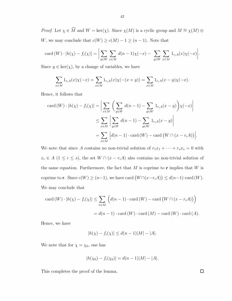
42

Proof. Let χ ∈ M and W = ker(χ). Since χ(M) is a cyclic group and M ∼= χ(M) ⊕

W , we may conclude that c(W ) ≥ c(M) − 1 ≥ (n− 1). Note that

card (W ) · |h(χ) − fi(χ)| =

∣∣∣∣∑

y∈W

∑

x∈M

d(n− 1)χ(−x) −∑

y∈W

∑

x∈M

1riA(x)χ(−x)

∣∣∣∣.

Since y ∈ ker(χ), by a change of variables, we have

∑

x∈M

1riA(x)χ(−x) =∑

x∈M

1riA(x)χ(−(x+ y)) =∑

x∈M

1riA(x− y)χ(−x).

Hence, it follows that

card (W ) · |h(χ) − fi(χ)| =

∣∣∣∣∑

x∈M

(∑

y∈W

d(n− 1) −∑

y∈W

1riA(x− y)

)χ(−x)

∣∣∣∣

≤∑

x∈M

∣∣∣∣∑

y∈W

d(n− 1) −∑

y∈W

1riA(x− y)

∣∣∣∣

=∑

x∈M

∣∣∣d(n− 1) · card (W ) − card(W ∩ (x− riA)

)∣∣∣.

We note that since A contains no non-trivial solution of r1x1 + · · · + rsxs = 0 with

xi ∈ A (1 ≤ i ≤ s), the set W ∩ (x − riA) also contains no non-trivial solution of

the same equation. Furthermore, the fact that M is coprime to r implies that W is

coprime to r. Since c(W ) ≥ (n−1), we have card(W∩(x−riA)

)≤ d(n−1)·card (W ).

We may conclude that

card (W ) · |h(χ) − fi(χ)| ≤∑

x∈M

(d(n− 1) · card (W ) − card

(W ∩ (x− riA)

))

= d(n− 1) · card (W ) · card (M) − card (W ) · card (A).

Hence, we have

|h(χ) − fi(χ)| ≤ d(n− 1)|M | − |A|.

We note that for χ = χ0, one has

|h(χ0) − fi(χ0)| = d(n− 1)|M | − |A|.

This completes the proof of the lemma.

43

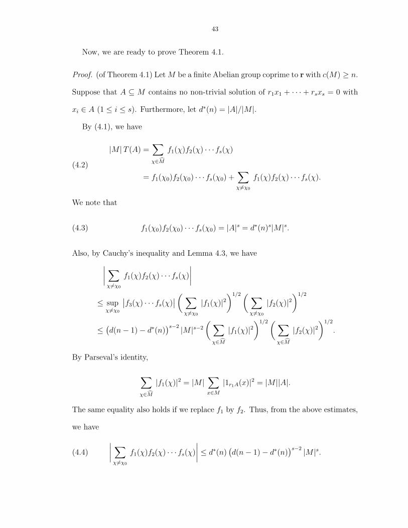
Now, we are ready to prove Theorem 4.1.

Proof. (of Theorem 4.1) LetM be a finite Abelian group coprime to r with c(M) ≥ n.

Suppose that A ⊆ M contains no non-trivial solution of r1x1 + · · · + rsxs = 0 with

xi ∈ A (1 ≤ i ≤ s). Furthermore, let d∗(n) = |A|/|M |.

By (4.1), we have

|M | T (A) =∑

χ∈M

f1(χ)f2(χ) · · ·fs(χ)

= f1(χ0)f2(χ0) · · ·fs(χ0) +∑

χ 6=χ0

f1(χ)f2(χ) · · ·fs(χ).

(4.2)

We note that

(4.3) f1(χ0)f2(χ0) · · · fs(χ0) = |A|s = d∗(n)s|M |s.

Also, by Cauchy’s inequality and Lemma 4.3, we have

∣∣∣∣∑

χ 6=χ0

f1(χ)f2(χ) · · ·fs(χ)

∣∣∣∣

≤ supχ 6=χ0

∣∣f3(χ) · · · fs(χ)∣∣( ∑

χ 6=χ0

|f1(χ)|2)1/2( ∑

χ 6=χ0

|f2(χ)|2)1/2

≤(d(n− 1) − d∗(n)

)s−2|M |s−2

(∑

χ∈M

|f1(χ)|2)1/2(∑

χ∈M

|f2(χ)|2)1/2

.

By Parseval’s identity,

∑

χ∈M

|f1(χ)|2 = |M |∑

x∈M

|1r1A(x)|2 = |M ||A|.

The same equality also holds if we replace f1 by f2. Thus, from the above estimates,

we have

(4.4)

∣∣∣∣∑

χ 6=χ0

f1(χ)f2(χ) · · · fs(χ)

∣∣∣∣ ≤ d∗(n)(d(n− 1) − d∗(n)

)s−2|M |s.

44

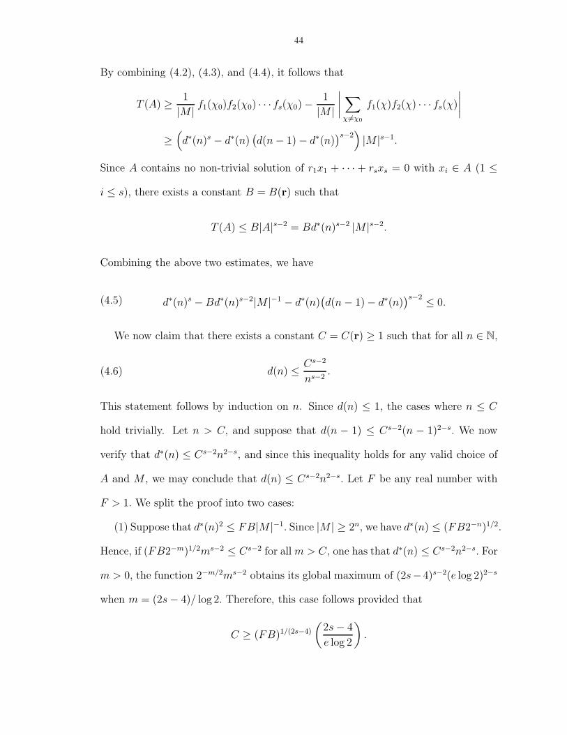
By combining (4.2), (4.3), and (4.4), it follows that

T (A) ≥1

|M |f1(χ0)f2(χ0) · · · fs(χ0) −

1

|M |

∣∣∣∣∑

χ 6=χ0

f1(χ)f2(χ) · · · fs(χ)

∣∣∣∣

≥(d∗(n)s − d∗(n)

(d(n− 1) − d∗(n)

)s−2)|M |s−1.

Since A contains no non-trivial solution of r1x1 + · · · + rsxs = 0 with xi ∈ A (1 ≤

i ≤ s), there exists a constant B = B(r) such that

T (A) ≤ B|A|s−2 = Bd∗(n)s−2 |M |s−2.

Combining the above two estimates, we have

d∗(n)s − Bd∗(n)s−2|M |−1 − d∗(n)(d(n− 1) − d∗(n)

)s−2≤ 0.(4.5)

We now claim that there exists a constant C = C(r) ≥ 1 such that for all n ∈ N,

(4.6) d(n) ≤Cs−2

ns−2.

This statement follows by induction on n. Since d(n) ≤ 1, the cases where n ≤ C

hold trivially. Let n > C, and suppose that d(n − 1) ≤ Cs−2(n − 1)2−s. We now

verify that d∗(n) ≤ Cs−2n2−s, and since this inequality holds for any valid choice of

A and M , we may conclude that d(n) ≤ Cs−2n2−s. Let F be any real number with

F > 1. We split the proof into two cases:

(1) Suppose that d∗(n)2 ≤ FB|M |−1. Since |M | ≥ 2n, we have d∗(n) ≤ (FB2−n)1/2.

Hence, if (FB2−m)1/2ms−2 ≤ Cs−2 for all m > C, one has that d∗(n) ≤ Cs−2n2−s. For

m > 0, the function 2−m/2ms−2 obtains its global maximum of (2s−4)s−2(e log 2)2−s

when m = (2s− 4)/ log 2. Therefore, this case follows provided that

C ≥ (FB)1/(2s−4)

(2s− 4

e log 2

).

45

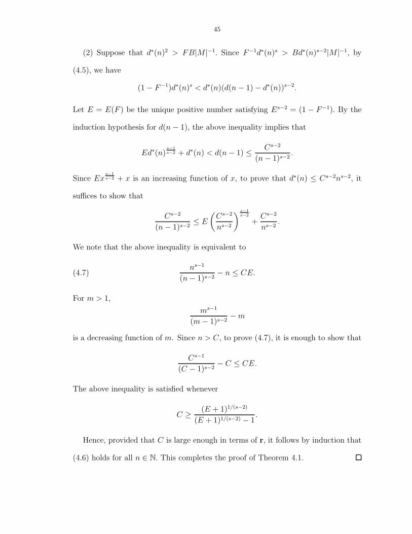
(2) Suppose that d∗(n)2 > FB|M |−1. Since F−1d∗(n)s > Bd∗(n)s−2|M |−1, by

(4.5), we have

(1 − F−1)d∗(n)s < d∗(n)(d(n− 1) − d∗(n))s−2.

Let E = E(F ) be the unique positive number satisfying Es−2 = (1 − F−1). By the

induction hypothesis for d(n− 1), the above inequality implies that

Ed∗(n)s−1s−2 + d∗(n) < d(n− 1) ≤

Cs−2

(n− 1)s−2.

Since Exs−1s−2 + x is an increasing function of x, to prove that d∗(n) ≤ Cs−2ns−2, it

suffices to show that

Cs−2

(n− 1)s−2≤ E

(Cs−2

ns−2

) s−1s−2

+Cs−2

ns−2.

We note that the above inequality is equivalent to

(4.7)ns−1

(n− 1)s−2− n ≤ CE.

For m > 1,

ms−1

(m− 1)s−2−m

is a decreasing function of m. Since n > C, to prove (4.7), it is enough to show that

Cs−1

(C − 1)s−2− C ≤ CE.

The above inequality is satisfied whenever

C ≥(E + 1)1/(s−2)

(E + 1)1/(s−2) − 1.

Hence, provided that C is large enough in terms of r, it follows by induction that

(4.6) holds for all n ∈ N. This completes the proof of Theorem 4.1.

46

Remark 4.4. We see from the above proof that our constant C = C(r) can be

computed explicitly. For any value of E such that 0 < E < 1, we may choose C to

be

max

{(B

1 − Es−2

)1/(2s−4)(2s− 4

e log 2

),

(E + 1)1/(s−2)

(E + 1)1/(s−2) − 1

},

where B = B(r) is chosen as in the proof of Theorem 1. For any choice of r =

(r1, . . . , rs), one can numerically choose E to minimize the above expression. We

note that

lims→∞

((E + 1)1/(s−2)

(E + 1)1/(s−2) − 1−

s− 2

log(E + 1)−

1

2

)= 0.

Thus, for fixed B, the constant C can be chosen in such a way that it grows like a

linear function in s.

Remark 4.5. If the vector r = (r1, . . . , rs) ∈ Zs satisfies the condition that there is

no proper subset {j1, . . . , jl} ( {1, . . . , s} with rj1 + · · · + rjl= 0, then a solution

x = (x1, . . . , xs) ∈ As is trivial if and only if x1 = · · · = xs. Hence, T (A) = |A|, and

in place of (4.5), we obtain the inequality

d∗(n)s − d∗(n)|M |2−s − d∗(n)(d(n− 1) − d∗(n)

)s−2≤ 0.

By an argument similar to the proof of Theorem 4.1, for any value of E such that

0 < E < 1, we may choose C to be

max

{(1

1 − Es−2

) 1(s−1)(s−2)

(s− 1

e log 2

),

(E + 1)1/(s−2)

(E + 1)1/(s−2) − 1

}.

We note that in this case, the constant C depends only on s. Moreover, we can

change the constant E as n varies in our proof, i.e., E = E(n) can be chosen to be

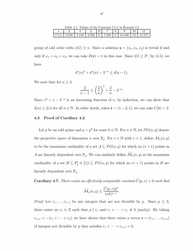
a function of n. Table 4.1 lists valid choices of C(s) for small values of s.

Remark 4.6. One can also optimize the choice of C = C(r) by utilizing the inequality

in (4.5) directly. Consider the special case that r = (1,−2, 1) andG is a finite Abelian

47

Table 4.1: Values of the Constant C(s) in Remark 4.5s 3 4 5 6 7 8 9 10 11

C(s) 2.050 3.138 4.766 6 7.598 9 10.436 12 13.277

group of odd order with c(G) ≥ n. Since a solution x = (x1, x2, x3) is trivial if and

only if x1 = x2 = x3, we can take B(r) = 1 in this case. Since |G| ≥ 3n, by (4.5), we

have

d∗(n)2 + d∗(n) − 3−n ≤ d(n− 1).

We note that for n ≥ 3,

2

n− 1≤

(2

n

)2

+2

n− 3−n.

Since x2 + x − 3−n is an increasing function of x, by induction, we can show that

d(n) ≤ 2/n for all n ∈ N. In other words, when r = (1,−2, 1), we can take C(r) = 2.

4.3 Proof of Corollary 4.2

Let p be an odd prime and q = ph for some h ∈ N. For n ∈ N, let PG(n, q) denote

the projective space of dimension n over Fq. For v ∈ N with v > 1, define Mv(n, q)

to be the maximum cardinality of a set A ⊆ PG(n, q) for which no (v + 1) points in

A are linearly dependent over Fq. We can similarly define Mv(n, q) as the maximum

cardinality of a set B ⊆ Fnq ⊕ {1} ⊆ PG(n, q) for which no (v + 1) points in B are

linearly dependent over Fq.

Corollary 4.7. There exists an effectively computable constant C(p, v) > 0 such that

Mv(n, q) ≤C(p, v)qn

(nh)v−1.

Proof. Let r1, . . . , rv−1 be any integers that are not divisible by p. Since p ≥ 3,

there exists an rv ∈ Z such that p ∤ rv and r1 + · · · + rv 6≡ 0 (mod p). By taking

rv+1 = −(r1 + · · · + rv), we have shown that there exists a vector r = (r1, . . . , rv+1)

of integers not divisible by p that satisfies r1 + · · · + rv+1 = 0.

48

Suppose that B ⊆ Fnq ⊕ {1} and no (v + 1) points in B are linearly dependent

over Fq. Let r = (r1, . . . , rv+1) be a vector of integers not divisible by p that satisfies

r1+· · ·+rv+1 = 0. If B contains a non-trivial solution of r1x1+· · ·+rv+1xv+1 = 0 with

xi ∈ B (1 ≤ i ≤ v+1), then there are (v+1) points in B that are linearly dependent

over Fq. Hence, by viewing Fnq as a finite Abelian group with nh constituents, we

can derive from Theorem 4.1 that

(4.8) Mv(n, q) ≤C(r)v−1 qn

(nh)v−1.

Define

C(p, v) = infr

{C(r)v−1

},

where r runs through all vectors (r1, . . . , rv+1) of integers not divisible by p with

r1 + · · ·+ rv+1 = 0. Then, by (4.8), the corollary follows.

We are now ready to prove Corollary 4.2, which states that

Mv(n, q) ≤C(p, v)

hv−1·

n∑

j=1

qj

jv−1+ 1.

Proof. (of Corollary 4.2) We note that an element of PG(n, q) can be written either

as (y, 1) with y ∈ Fnq or as (z, 0) with z ∈ PG(n− 1, q). Thus, for n ≥ 1, we have

(4.9) Mv(n, q) ≤ Mv(n, q) + Mv(n− 1, q).

We note that

(4.10) Mv(1, q) ≤ Mv(1, q) + 1.

By (4.9), (4.10), and Corollary 4.7, we have

Mv(n, q) ≤n∑

j=1

Mv(j, q) + 1 ≤C(p, v)

hv−1·

n∑

j=1

qj

jv−1+ 1.

The corollary now follows.

CHAPTER V

The Manin Conjecture for x0y0 + · · · + xsys = 0

5.1 Overview

We consider the variety defined by x0y0 + · · · + xsys = 0 in Ps(Q) × Ps(Q). This

is a flag variety with anticanonical height function

(5.1) H(x,y) = max0≤i,j≤s

|xiyj|s,

where we choose representatives x = (x0, . . . , xs) ∈ Zs+1 and y = (y0, . . . , ys) ∈ Zs+1

with gcd(x0, . . . , xs) = gcd(y0, . . . , ys) = 1. Let

N(B) = #{(x,y) ∈ Ps(Q) × Ps(Q) : x · y = 0, x0 · · ·xsy0 · · · ys 6= 0,

and H(x,y) < B}.(5.2)

For the variety x0y0 + · · · + xsys = 0, the Manin conjecture predicts that N(B) ∼

κB logB, where κ is a constant.

We first need to define some notation. Let x = (x0, . . . , xs) and y = (y0, . . . , ys) be

vectors lying in Rs+1. For the sake of concision, we write xi for (x0, . . . , xi−1, xi+1, . . . , xs)

and likewise yi for (y0, . . . , yi−1, yi+1, . . . , ys). Furthermore, for any vector u, we de-

fine ‖u‖∞ = max |ui|, where the maximum is taken over all components ui of u.

Let

X1 = {(x0,y0) ∈ R2s : ‖x0‖∞ ≤ 1, ‖y0‖∞ ≤ 1, and |x0 · y0| ≤ 1}.

49

50

We define the local density at infinity to be

(5.3) σ∞ =

∫

X1

dx0 dy0,

and the singular series to be

S =

∞∑

q=1

φ(q)

qs+1.

Note that for s ≥ 2, we have S ≪ 1.

In this chapter, we prove the following theorem.

Theorem 5.1. For s ≥ 2 and B ≥ 2, we have

N(B) =

(s+ 1

2s

)ζ(s)−2σ∞SB logB +O(B).

Let

W = {(x,y) ∈ (Z \ {0})2s+2 : y0 > 0, ‖y‖∞ ≤ y0 ≤ B1/2, and ‖x‖∞ ≤ B/y0}

and

N0(B) = #{(x,y) ∈ W : x · y = 0}.

In order to verify Theorem 5.1, we prove the following theorem.

Theorem 5.2. For s ≥ 2 and B ≥ 2, one has

N0(B) =1

2σ∞SBs logB +O(Bs).

Let e(α) = exp(2πα) and

(5.4) F(α) =∑

(x,y)∈W

e(αx · y).

Let δ > 0 be a small positive constant with δ < 1/10, and let Q = Bδ. We define

M(a, q) = {α ∈ R : |α− a/q| ≤ B−1Q}.

51

The major arcs are defined to be

M =⋃

1≤a≤q≤Q(a,q)=1

M(a, q),

and the minor arcs are

m =[B−1Q, 1 +B−1Q

)\ M.

Note that when 1 ≤ a1 ≤ q1 ≤ Q and 1 ≤ a2 ≤ q2 ≤ Q with (a1, q1) = (a2, q2) = 1,

we have M(a1, q1)∩M(a2, q2) 6= ∅ if and only if a1 = a2 and q1 = q2. Thus, the major

arcs M(a, q) that constitute M are disjoint. Since

∫

T

e(αn) dα =

1, when n = 0,

0, when n ∈ Z\{0},

where T = [0, 1), we have

N0(B) =

∫ 1+B−1Q

B−1Q

F(α) dα.

In order to prove Theorem 5.2, it now suffices to demonstrate that for B ≥ 2, one

has

(5.5)

∫

m

F(α) dα = O(Bs+ǫQ−1)

and

(5.6)

∫

M

F(α) dα =1

2σ∞SBs logB +O(Bs).

We prove (5.5) in Section 5.2 and (5.6) in Section 5.3. In Section 5.4, we derive

Theorem 5.1 from Theorem 5.2.

This chapter is based on the author’s preliminary manuscript [36].

52

5.2 The Minor Arcs

Our goal for this section is to prove (5.5). We first record a reciprocal sum estimate

and a version of Hua’s inequality. In this section, we write ‖α‖ for the fractional

part of α.

Lemma 5.3. Suppose that X and Y are real numbers with X ≥ 1 and Y ≥ 1. Also,

suppose that a ∈ Z, q ∈ N, and α ∈ R satisfy |α− a/q| ≤ q−2 and (a, q) = 1. Then,

∑

1≤y≤Y

min(XY

y, ‖αy‖−1

)≪ XY

(1

q+

1

X+

q

XY

)log(2Y q).

Proof. See [44, Lemma 2.2].

Lemma 5.4. One has

(5.7) #{(x, x′, y, y′) ∈ Z4 : 1 ≤ |xy| = |x′y′| ≤ B} ≪ B1+ǫ.

Proof. For a natural number n, let τ2(n) denote the number of positive integers that

divide n. A standard divisor function estimate (see, for example, the argument on

page 10 of [7]) shows that τ2(n) ≪ nǫ, and hence,

#{(x, x′, y, y′) ∈ Z4 : 1 ≤ |xy| = |x′y′| ≤ B} ≪∑

1≤n≤B

(τ2(n))2

≪∑

1≤n≤B

nǫ ≪ B1+ǫ.

With greater effort, in fact, one may obtain an upper bound for the left hand

side of (5.7) of the shape O(B(logB)3

)(see [21, Lemma 2.5]). We are now in a

position to show that the minor arc contribution is O(Bs+ǫQ−1), thereby confirming

(5.5). One difficulty that arises in the proof is that F(α) does not naturally break

apart into a product of s exponential sums owing to dependencies on y0. In order to

get around this, we employ a standard argument from the theory of Fourier analysis

53

to de-interlace the pairs (xi, yi) (see the appendix due to Montgomery in [48]). We

define

g(α, γ, η) =∑

x,y1≤|xy|≤B

e(αxy − γx− ηy).

Let

DR(γ) =∑

1≤|z|≤R

e(γz),

and note that for positive real numbers R and S with RS ≤ B, we have

(5.8)

∫

T2

g(α, γ, η)DR(γ)DS(η) dγ dη =∑

1≤|x|≤R1≤|y|≤S

e(αxy).

Lemma 5.5. For s ≥ 2, one has

∫

m

F(α) dα = O(Bs+ǫQ−1).

Proof. Denote by γ = (γ1, . . . , γs) and η = (η1, . . . , ηs) vectors lying in Ts. Let

G(α,γ,η) =∑

1≤y0≤B1/2

1≤|x0|≤B/y0

e(αx0y0)s∏

i=1

g(α, γi, ηi)Dy0(γi)DB/y0(ηi).

By using (5.8), we are able to rewrite F(α) as

(5.9) F(α) =

∫

Ts

∫

Ts

G(α,γ,η) dγ dη.

Let

C =[B−2s−2, 1 − B−2s−2

]s.

Using trivial estimates, we find that

(5.10) g(α, γ, η) ≪∑

x,y1≤|xy|≤B

1 ≪∑

1≤y≤B

B/y ≪ B logB

and

Dy0(γ)DB/y0(η) ≪ y0(B/y0) = B

54

uniformly in α, γ, and η. Hence, we have

(5.11) G(α,γ,η) ≪ B2s+1(logB)s+1 ≪ B2s+2

uniformly in α, γ, and η. The measure of (Ts × Ts) \ (C × C) equals the volume of

the boundary shell, which is O(B−2s−2). Hence, together with (5.9) and (5.11), we

obtain

(5.12)

∫

m

F(α) dα =

∫

m

∫

C

∫

C

G(α,γ,η) dγ dη dα +O(1).

When γ /∈ Z and R ≥ 1, one finds by summing the geometric progressions that

(5.13) DR(γ) =e(γ) − e(⌊R + 1⌋γ) + e(−⌊R⌋γ) − 1

1 − e(γ).

Let

D∗(γ,η) =s∏

i=1

(1

1 − e(γi)

)(1

1 − e(ηi)

).

By applying (5.13), we find that there exists a complex number ρ(B, y0,γ,η), inde-

pendent of x0 and of modulus at most 42s, such that

(5.14)

s∏

i=1

Dy0(γi)DB/y0(ηi) = ρ(B, y0,γ,η)D∗(γ,η)

for all (γ,η) ∈ C2. Hence, for all (γ,η) ∈ C2, we may write

(5.15) G(α,γ,η) = D∗(γ,η)h(α,B,γ,η)

(s∏

j=1

g(α, γj, ηj)

),

where

h(α,B,γ,η) =∑

1≤y0≤B1/2

ρ(B, y0,γ,η)∑

1≤|x0|≤B/y0

e(αx0y0).

By the triangle inequality, we find that

h(α,B,γ,η) ≤ 42s∑

1≤y0≤B1/2

∣∣∣∣∣∣∑

1≤|x0|≤B/y0

e(αx0y0)

∣∣∣∣∣∣

≪∑

1≤y0≤B1/2

max(B/y0, ‖αy0‖

−1)

55

uniformly in γ and η. By Dirichlet’s approximation theorem, for every α ∈ R, there

exist elements a, q ∈ Z such that 1 ≤ q ≤ BQ−1, (a, q) = 1, and |α−a/q| < q−1B−1Q.

If α ∈ m, for such a choice of a and q, we must have that q > Q and |α − a/q| <

q−1B−1Q ≤ q−2. Therefore, an application of Lemma 5.3 with X = Y = B1/2 implies

that

(5.16) h(α,B,γ,η) ≪ BQ−1 logB

uniformly in γ,η, and α ∈ m. From (5.10), (5.15), and (5.16), we may conclude that

∫

m

∫

C

∫

C

G(α,γ,η) dγ dη dα

≪ Bs−1Q−1(logB)s−1

∫

C

∫

C

∣∣D∗(γ,η)∣∣∫

m

2∏

j=1

|g(α, γj, ηj)| dαdγ dη.

(5.17)

On making use of orthogonality, it follows from Lemma 5.4 that

∫

T

|g(α, γ, η)|2 dα≪∑

x,x′,y,y′

1≤|xy|=|x′y′|≤B

1 ≪ B1+ǫ.

Hence, by Schwarz’s inequality, we find that

∫

m

2∏

j=1

|g(α, γj, ηj)| dα ≤2∏

j=1

(∫

T

|g(α, γj, ηj)|2 dα

)1/2

≪ B1+ǫ.

From (5.17), we now have that

(5.18)

∫

m

∫

C

∫

C

G(α,γ,η) dγ dη dα≪ Bs+ǫQ−1

∫

C

∫

C

∣∣D∗(γ,η)∣∣ dγ dη.

Observe that∫ 1−B−2s−2

B−2s−2

dβ

1 − e(β)≪

∫ 1−B−2s−2

B−2s−2

dβ

‖β‖≪ logB,

which implies that

(5.19)

∫

C

∫

C

∣∣D∗(γ,η)∣∣ dγ dη ≪ (logB)2s ≪ Bǫ.

56

Combining (5.12), (5.18), and (5.19) yields the upper bound

∫

m

F(α) dα≪ Bs+ǫQ−1.

This completes the proof of the lemma.

5.3 The Major Arcs

In order to prove (5.6), we first prove an auxiliary lemma. Throughout this section,

when α ∈ M(a, q), we write β = α− a/q.

Lemma 5.6. When α ∈ M(a, q), y ∈ Z, and X ≥ 1, we have

∑

1≤|x|≤X

e(αxy) = q−1

q∑

u=1

e

(a

quy

)∫ X

−X

e(βxy) dx+O(q(1 + |β|Xy)).

Proof. By splitting the sum into arithmetic progressions modulo q, we have

∑

1≤|x|≤X

e(αxy) =

q∑

u=1

e

(a

quy

) ∑

|x|≤Xx≡u (mod q)

e(βxy) +O(1)

=

q∑

u=1

e

(a

quy

) ∑

r∈Z

|qr+u|≤X

e(β(qr + u)y) +O(1)(5.20)

=

q∑

u=1

e

(a

quy

) ∑

q−1(−X−u)≤r≤q−1(X−u)

e(β(qr + u)y) +O(1).

The inner sum may be replaced with an integral by noting that from the mean value

theorem,

∑

q−1(−X−u)≤r≤q−1(−X−u)

e(β(qr + u)y) =

∫ (X−u)/q

(−X−u)/q

e(β(qr + u)y) dr

+O(1 + q−1X max

q−1(−X−u)≤r≤q−1(X−u)|βqy|

)

= q−1

∫ X

−X

e(βxy) dx+O(1 + |βXy|).

Therefore, we may conclude from (5.20) that

∑

1≤|x|≤X

e(αxy) = q−1

q∑

u=1

e

(a

quy

)∫ X

−X

e(βxy) dx+O(q(1 + |βXy|)

).

57

Define

V1 = {y ∈ Zs+1 : 1 ≤ |y1|, . . . , |ys| ≤ y0 ≤ B1/2}

and

X2 = {x ∈ Rs+1 : ‖x‖∞ ≤ B/y0}.

Let

(5.21) S(a, q,y) =∑

x (mod q)

(a

qx · y

)

and

(5.22) T (y) =

∫ B−1Q

−B−1Q

∫

X2

e(βx · y) dx dβ.

Lemma 5.7. For s ≥ 2, one has

∫

M

F(α) dα =∑

1≤a≤q≤Q(a,q)=1

∑

y∈V1

q−1−sS(a, q,y)T (y) +O(Bs).

Proof. For α ∈ M(a, q), by Lemmas 5.6, we have that

F(α) =∑

y∈V1

J(α, y0, y0) · · ·J(α, y0, ys),

where

J(α, y0, y) = q−1

q∑

u=1

e

(a

quy

)∫ B/y0

−B/y0

e(βxy) dx+O(q(1 + |β|B)).

Note that for α ∈ M(a, q), we have

q(1 + |β|B) ≪ qQ.

In addition, the trivial estimate |e(z)| ≤ 1 for z ∈ R yields

q−1

q∑

u=1

e

(a

quy

)∫ B/y0

−B/y0

e(βxy) dx≪ B/y0.

58

Therefore, we may write

∫

M

F(α) dα−∑

1≤a≤q≤Q(a,q)=1

∑

y∈V1

q−1−sS(a, q,y)T (y) ≪ E1 + E2,

where

E1 =∑

1≤a≤q≤Q(a,q)=1

∑

y∈V1

∫ B−1Q

−B−1Q

(qQ)s+1 dβ

and

E2 =∑

1≤a≤q≤Q(a,q)=1

∑

y∈V1

∫ B−1Q

−B−1Q

(qQ)(B/y0)s dβ.

Noting that the measure of the domain of integration is O(B−1Q), we observe that

E1 ≪ B−1Qs+2∑

1≤q≤Q

qs+2∑

1≤y0≤B1/2

ys0 ≪ B(s−1)/2Q2s+5,

and

E2 ≪ Bs−1Q2∑

1≤q≤Q

q2∑

1≤y0≤B1/2

1 ≪ Bs−1/2Q5.

Recalling that we chose Q to be Bδ and δ < 1/10, we may conclude that E1 +E2 ≪

Bs. This completes the proof of the lemma.

Let

(5.23) X3(y) = {x0 ∈ Rs : ‖x0‖∞ ≤ 1 and |x1y1/y0 + · · · + xsys/y0| ≤ 1}.

Lemma 5.8. For s ≥ 2, one has

T (y) = Bsy−1−s0

∫

X3(y)

dx0 +O

(Bs

Qs|y0 · · · ys|

).

Proof. Let

G(x,y) = x0 + x1y1

y0+ · · · + xs

ys

y0

and

X4 = {x ∈ Rs+1 : ‖x‖∞ ≤ 1}.

59

By a change of variables in the right hand side of (5.22), namely x → (B/y0)x and

β → B−1β, we have

T (y) = Bsy−1−s0

∫ Q

−Q

∫

X4

e(βG(x,y)) dxdβ.

Since∫ D

C

e(γx) dx≪ min(|D − C|, |γ|−1),

for γ 6= 0, it follows that when yi 6= 0 for 0 ≤ i ≤ s, we have

∫

|β|>Q

∫

X4

e(βG(x,y)) dxdβ ≪

∫

|β|>Q

ys0

|βs+1y1 · · · ys|dβ ≪

ys0

Qs|y1 · · · ys|.

Therefore, we have

T (y) = Bsy−1−s0

∫ ∞

−∞

∫

X4

e(βG(x,y)) dxdβ +O

(Bs

Qs|y0 · · · ys|

).

Let

X5(y, u) = {x0 ∈ Rs : ‖x0‖∞ ≤ 1 and |u− (x1y1/y0 + · · ·+ xsys/y0)| ≤ 1}.

Observing that∫ λ

−λ

e(βu) dβ =sin(2πλu)

πu

for u 6= 0 and making a change of variables, namely

x0 → (u− x1y1/y0 − · · · − xsys/y0),

we may conclude that

∫ ∞

−∞

∫

X4

e(βG(x,y)) dxdβ = limλ→∞

∫

X4

sin(2πλG(x,y))

πG(x,y)dx

= limλ→∞

∫ s+1

−s−1

ψ2(y, u)sin(2πλu)

πudu,(5.24)

where

ψ2(y, u) =

∫

X5(y,u)

dx0.

60

We note that if u is not in the interval

[− 1 − (|y1| + · · · + |ys|)/y0, 1 + (|y1| + · · ·+ |ys|)/y0

],

then X5(y, u) is empty, and hence ψ2(y, u) = 0. The latter values of u consequently

make no contribution in the last integral in (5.24). By the Fourier Integral Theorem,

we have that∫ ∞

−∞

∫

X4

e(βG(x,y)) dxdβ = ψ2(y, 0).

On noting from (5.23) that X5(y, 0) = X3(y), it now follows that

ψ2(y, 0) =

∫

X3(y)

dx0,

which completes the proof of our lemma.

It is convenient to have available the following technical lemma in order to more

concisely estimate the major arc contribution in Lemma 5.10.

Lemma 5.9. Let I0 = [−1, 1] and

I(z, y0, K) = {x ∈ R : |xz/y0 −K| ≤ 1}.

Suppose that 0 ≤ |y| − 1 ≤ |y′| ≤ |y| ≤ y0. Then, for any real number K, one has

∣∣∣∣∫

I0∩I(y′,y0,K)

dx−

∫

I0∩I(y,y0,K)

dx

∣∣∣∣ ≤ 4/|y|.

Proof. Since ∣∣∣∣∫

I0∩I(y′,y0,K)

dx−

∫

I0∩I(y,y0,K)

dx

∣∣∣∣ ≤ 2

it suffices to prove this lemma under the assumption that |y| > 2. By symmetry, we

may also assume that 1 < y′ ≤ y ≤ y0 and K ≥ 0. Observe that for z > 0, we have

I(z, y0, K) =

[y0(K − 1)

z,y0(K + 1)

z

].

61

We now divide our work into two cases: 0 ≤ K ≤ 1 and K > 1.

(i) Suppose that 0 ≤ K ≤ 1. The relation 1 < y′ ≤ y ≤ y0 implies that

y0(K − 1)

y′≤y0(K − 1)

y≤ 0 < 1 ≤

y0(K + 1)

y≤y0(K + 1)

y′.

Hence,

I0 ∩ I(y, y0, K) ⊆ I0 ∩ I(y′, y0, K),

and so∫

I0∩I(y,y0,K)

dx ≤

∫

I0∩I(y′,y0,K)

dx.

Furthermore, we have that

∫

I0∩I(y,y0,K)

dx = 1 + min

(1,y0(1 −K)

y

)

and that∫

I0∩I(y′,y0,K)

dx = 1 + min

(1,y0(1 −K)

y′

).

If

1 ≤y0(1 −K)

y,

then∫

I0∩I(y,y0,K)

dx = 2 =

∫

I0∩I(y′,y0,K)

dx.

If, on the other hand,

y0(1 −K)

y< 1,

then

0 ≤

∫

I0∩I(y′,y0,K)

dx−

∫

I0∩I(y,y0,K)

dx = min

(1,y0(1 −K)

y′

)−y0(1 −K)

y

≤y0(1 −K)

y′−y0(1 −K)

y

=y0(1 −K)(y − y′)

yy′≤y0(y/y0)

yy′

= 1/y′ ≤ 2/y.

62

(ii) Now suppose that K > 1. The relation 1 < y′ ≤ y ≤ y0 implies that

0 <y0(K − 1)

y≤y0(K − 1)

y′

and

1 ≤y0(K + 1)

y≤y0(K + 1)

y′.

Therefore,

I0 ∩ I(y′, y0, K) ⊆ I0 ∩ I(y, y0, K),

which implies that∫

I0∩I(y′,y0,K)

dx ≤

∫

I0∩I(y,y0,K)

dx.

Also, we see that

∫

I0∩I(y,y0,K)

dx = 1 − min

(1,y0(K − 1)

y

)

and∫

I0∩I(y′,y0,K)

dx = 1 − min

(1,y0(K − 1)

y′

).

If

1 ≤y0(K − 1)

y,

then∫

I0∩I(y,y0,K)

dx = 0 =

∫

I0∩I(y′,y0,K)

dx.

If, on the other hand,

y0(K − 1)

y< 1,

63

then

0 ≤

∫

I0∩I(y,y0,K)

dx−

∫

I0∩I(y′,y0,K)

dx = min

(1,y0(K − 1)

y′

)−y0(K − 1)

y

≤y0(K − 1)

y′−y0(K − 1)

y

=y0(K − 1)(y − y′)

yy′≤y0(y/y0)

yy′

= 1/y′ ≤ 2/y.

This completes the proof of our lemma.

Lemma 5.10. For s ≥ 2, one has

∫

M

F(α) dα =1

2σ∞SBs logB +O(Bs).

Proof. Let

V2(q) = {y ∈ Zs+1 : 1 ≤ |y1|, . . . , |ys| ≤ y0 ≤ B1/2 and q| gcd(y0, . . . , ys)}

and

V3(q) = {y ∈ Zs+1 : 1 ≤ |y1|, . . . , |ys| ≤ y0 ≤ q−1B1/2}.

Note that from (5.21),

S(a, q,y) =∑

x (mod q)

(aqx · y

)=

qs+1, when q | gcd(y0, . . . , ys),

0, when q ∤ gcd(y0, . . . , ys).

64

By Lemmas 5.7 and 5.8, we have

∫

M

F(α) dα− Bs∑

1≤a≤q≤Q(a,q)=1

∑

y∈V2(q)

y−1−s0

∫

X3(y)

dx0

≪ Bs +BsQ−s∑

1≤a≤q≤Q(a,q)=1

∑

y∈V2(q)

|y0 · · · ys|−1

≪ Bs +BsQ−s∑

1≤q≤Q

q−s∑

y∈V3(q)

|y0 · · · ys|−1

≪ Bs,

and hence, in view of the definitions of V2(q), V3(q), and X3(y), one has

(5.25)

∫

M

F(α) dα = Bs∑

1≤a≤q≤Q(a,q)=1

q−1−s∑

y∈V3(q)

y−1−s0

∫

X3(y)

dx0 +O(Bs).

Let

X6(y0) = {(x0,y0) ∈ R2s : ‖x0‖∞ ≤ 1, ‖y0‖∞ ≤ y0, and

|x1y1/y0 + · · ·+ xsys/y0| ≤ 1}.

Observe that for K ∈ R and y0 ≥ 1, by Lemma 5.9 and the mean value theorem, we

have

∑

1≤|y|≤y0

∫|x|≤1

|xy/y0−K|≤1

dx−

∫|x|≤1, |y|≤y0

|xy/y0−K|≤1

dx dy ≪∑

1≤|y|≤y0

4/|y|

≪ log(2y0).

We may iteratively apply the above inequality s times to exchange our sum over yi

for an integral over yi for each 1 ≤ i ≤ s. By carrying out this procedure and noting

that∫

X3(y)

dx0 ≤ 2s,

65

we obtain that

∑

y∈V3(q)

y−1−s0

∫

X3(y)

dx0 −∑

y0≤q−1B1/2

y−1−s0

∫

X6(y0)

dx0 dy0 ≪∑

y0≤q−1B1/2

log y0

y20

≪ 1.(5.26)

Furthermore, by making the change of variables y0 → y0y0 and recalling (5.3), one

has

(5.27)∑

y0≤q−1B1/2

y−1−s0

∫

X6(y0)

dx0 dy0 = σ∞∑

y0≤q−1B1/2

y−10 .

Combining (5.25), (5.26), and (5.27), we have now shown that

∫

M

F(α) dα = σ∞Bs∑

1≤a≤q≤Q(a,q)=1

q−1−s∑

y0≤q−1B1/2

y−10 +O

(Bs

∑

1≤q≤Q

q−s

)

= σ∞Bs∑

1≤a≤q≤Q(a,q)=1

q−1−s

(1

2logB − log q +O(1)

)+O(Bs).

=1

2σ∞B

s logB∑

1≤q≤Q

φ(q)

qs+1+O(Bs).

On observing that∑

1≤q≤Q

φ(q)

qs+1= S +O(Q1−s),

we now find that∫

M

F(α) dα =1

2σ∞SBs logB +O(Bs).

Theorem 5.2 now follows from Lemmas 5.5 and 5.10.

5.4 The Proof of Theorem 5.1

Now that we have completed our proof of Theorem 5.2, we are able to derive

Theorem 5.1. Let

U(B) = {(x,y) ∈ (Z \ {0})2s+2 : x · y = 0 and maxi,j

|xiyj| ≤ B}

66

and N1(B) = #U(B). We first prove two auxiliary lemmas. Then, we derive an

asymptotic formula for N1(B), and we conclude by applying our asymptotic formula

for N1(B) in combination with Mobius inversion to prove Theorem 5.1.

Lemma 5.11. For s ≥ 2, one has

#{

(x,y) ∈(Z ∩ [−B1/2, B1/2]

)2s+2: x · y = 0

}≪ Bs.

Proof. Note that

xy =1

4

((x+ y)2 − (x− y)2

)

and that the mapping L : Z2 → Z2, defined by L(x, y) = (x+ y, x− y), is injective.

Hence, by setting (ui, vi) = (xi + yi, xi − yi), the set

{(x,y) ∈

(Z ∩ [−B1/2, B1/2]

)2s+2: x · y = 0

}

injects into the set

{(u,v) ∈

(Z ∩ [−2B1/2, 2B1/2]

)2s+2: (u2

0 − v20) + · · ·+ (u2

s − v2s) = 0

}.

The size of the above set is equal to

∫

T

|H(B)|2s+2 dα,

where

H(B) =∑

0≤z≤2B1/2

e(αz2).

Since (2s+ 2) ≥ 6, it follows from Chapter 2 of [44] that

∫

T

|H(B)|2s+2 dα≪(2B1/2

)2s≪ Bs.

The lemma now follows.

67

Lemma 5.12. For s ≥ 2, B ≥ 2, and i ∈ {0, . . . , s}, one has

#{(x,y) ∈ U(B) : |yi| = maxj

|yj| ≤ B1/2 and max0≤k<i

|yk| < |yi|}

= σ∞SBs logB +O(Bs).

Proof. One can follow the argument of our proof of Theorem 5.2 mutatis mutandis

to show that

#{(x,y) ∈ U(B) : yi = maxj

|yj| ≤ B1/2 and max0≤k<i

|yk| < yi}

=1

2σ∞SBs logB +O(Bs).

The lemma now follows by noting that

x · y = 0 ⇔ x · (−y) = 0

in order to account for both positive and negative values of yi.

Lemma 5.13. For s ≥ 2 and B ≥ 2, one has

N1(B) = (2s+ 2)σ∞SBs logB +O(Bs).

Proof. We first split the set U(B) into 2s+2 regions. Note that for each point in this

set, either maxi |xi| ≤ B1/2 or maxj |yj| ≤ B1/2. The 2s+ 2 regions that we consider

are K0, . . . ,Ks,L0, . . . ,Ls, where

Ki = {(x,y) ∈ U(B) : |xi| = maxj

|xj | ≤ B1/2 and max0≤k<i

|xk| < |xi|}

and

Li = {(x,y) ∈ U(B) : |yi| = maxj

|yj| ≤ B1/2 and max0≤k<i

|yk| < |yi|}.

Observe that when 0 ≤ k < l ≤ s, we have Kk ∩ Kl = ∅ = Lk ∩ Ll. Furthermore, for

k, l ∈ {0, . . . , s}, the intersection of Kk and Ll lies inside the set

{(x,y) ∈(Z ∩ [−B1/2, B1/2]

)2s+2: x · y = 0},

68

and so by Lemma 5.11, the size of Kk ∩ Ll is O(Bs).

By applying Lemma 5.12, we see that each of our 2s+2 regions K0, . . . ,Ks,L0, . . . ,Ls

is of size

σ∞SBs logB +O(Bs).

Hence, we have

N1(B) = (2s+ 2)σ∞SBs logB +O(Bs).

We now prove Theorem 5.1.

Proof. (of Theorem 5.1)

Recall the definitions of H(x,y) and N(B) in (5.1) and (5.2), respectively. When

counting the points that contribute to N(B) and N1(B), note that the height of a

solution differs by a power of s. Furthermore, for (x,y) ∈ Ps(Q) × Ps(Q), the def-

inition of our anticanonical height function H(x,y) assumes that gcd(x0, . . . , xs) =

gcd(y0, . . . , ys) = 1. Also, for (x,y) ∈ Ps(Q) × Ps(Q), we have (x,y) = (x,−y) =

(−x,y) = (−x,−y). Let M(B) = N(Bs). Hence,

N1(B) = 4∞∑

i=1

∞∑

j=1

M

(B

ij

),

and by Mobius inversion, we have that

M(B) =1

4

∞∑

i=1

∞∑

j=1

µ(i)µ(j)N1

(B

ij

)

=

(s+ 1

2

)σ∞S

∑

i,jij≤B

µ(i)µ(j)

(B

ij

)s

log

(B

ij

)+O

∑

i,jij≤B

Bs

isjs

=

(s+ 1

2

)σ∞SBs logB

∑

i,jij≤B

µ(i)µ(j)

isjs+O

B

s∑

i,jij≤B

log(ij)

isjs

.

69

Note that

Bs∑

i,jij≤B

log(ij)

isjs≪ Bs

and that

∑

i,jij≤B

µ(i)µ(j)

isjs=

∑

1≤i≤B1/2

µ(i)

is

2

+O

∑

1≤k≤B

1

ks

∑

l>B1/2

1

ls

=(ζ(s)−1 +O

(B(1−s)/2

))2

+O(B(1−s)/2

).

= ζ(s)−2 + O(B(1−s)/2).

Hence, we have

M(B) =

(s+ 1

2

)ζ(s)−2σ∞SBs logB +O(Bs),

which implies that

N(B) = M(B1/s) =

(s+ 1

2s

)ζ(s)−2σ∞SB logB +O(B).

This completes the proof of Theorem 5.1.

APPENDIX

70

71

APPENDIX A

Statement of Results Used in Chapter II

In this appendix, we provide statements of the lemmas used in Chapter II which

are from the preprints [28] and [27] of Liu and Wooley. The notation here will be

consistent with that of Chapter II, and we will assume that char(Fq) ∤ k.

Let

U(a, g) =∑

〈r〉<〈g〉

e(ark/g).

Lemma A.1. (i) Suppose that α ∈ T and that α = a/g + β with a, g ∈ Fq[t],

0 ≤ 〈a〉 < 〈g〉 ≤ P , and 〈β〉 < 〈g〉−1P 1−k. Then, F (α;P ) = 〈g〉−1U(a, g)F (β;P ).

(ii) When 〈β〉 < P 1−k, one has F (β;P ) ≪ P (1 + P k〈β〉)−1/k.

(iii) When (a, g) = 1, one has U(a, g) ≪ 〈g〉1−1/k.

Proof. This is Lemma 4.1 of [28].

Lemma A.2. Let P and R be positive numbers with P ≥ 1 and 2P/ log(2P ) < R <

P − logP . Suppose that α ∈ T, that a and g are elements of Fq[t] with g monic and

(a, g) = 1, and write β = α − a/g. Then, whenever 〈g〉 ≤ R and 〈β〉 < P 1−k, one

has

f(α;P,R) − 〈g〉−1U(a, g)ρ(P/R)F (β;P ) ≪ 〈g〉P (log P )−1/2(1 + P k〈β〉).

Proof. This is Lemma 4.3 of [28].

72

Lemma A.3. Suppose that u > 2k − 2 is accessible to the exponent k and that v is

an integer with 2v ≥ u. Then, we have

∫

T

|F (α)2f(α)2v| dα≪ P 2v+2−k.

Proof. This is Lemma 6.2 of [28].

Lemma A.4. There exists a positive absolute constant C such that if

u+ 5 ≥ sq,k + Ck√

Log Log k/Log k,

then u is accessible to the exponent k.

Proof. This is a combination of Theorem 9.4, Corollary 13.3, and Lemma 14.1 of

[28].

Lemma A.5. There exists a small positive constant ν = ν(q, k) such that

supα∈n

|F (α)| ≪ P 1−ν .

Proof. This is a theorem in [27].

BIBLIOGRAPHY

73

74

BIBLIOGRAPHY

[1] V. V. Batyrev and Y. Tschinkel, Manin’s conjecture for toric varieties, J. Alg. Geom. 7 (1998),1553.

[2] V. V. Batyrev and Y. Tschinkel, Rational points on some Fano cubic bundles, C. R. Acad. Sci.Paris 323 (1996), 41-46.

[3] V. Bentkus and F. Gotze, Lattice point problems and distribution of values of quadratic forms,

Ann. Math. 150 (1999), 977-1027.

[4] J. Bourgain, On triples in arithmetic progression, Geom. Funct. Anal. 9 (1999), 968-984.

[5] R. de la Breteche and T. D. Browning, On Manin’s conjecture for singular del Pezzo surfaces

of degree four, I, Mich. Math. J. 55 (2007), 51-80.

[6] R. de la Breteche and T. D. Browning, On Manin’s conjecture for singular del Pezzo surfaces

of degree four, II, Math. Proc. Cambridge Phil. Soc. 143 (2007), 579-605.

[7] H. Davenport, Analytic methods for Diophantine equations and Diophantine inequalities, 2nded., Cambridge Univ. Press, Cambridge, 2005.

[8] H. Davenport and H. Heilbronn, On indefinite quadratic forms in five variables, J. LondonMath. Soc. 21 (1946), 185-193.

[9] J. Franke, Y. Manin, and Y. Tschinkel, Rational points of bounded height on Fano varieties,Invent. Math. 95 (1989), 421-435.

[10] D. E. Freeman, Asymptotic lower bounds and formulas for Diophantine inequalities, NumberTheory for the Millennium, Vol. 2 (Urbana, IL, 2000), A. K. Peters, Natick, MA, 2002, 57-74.

[11] D. E. Freeman, Asymptotic lower bounds for Diophantine inequalities, Mathematika 47 (2000),127-159.

[12] W. T. Gowers, A new proof of Szemeredi’s theorem, Geom. Funct. Anal. 11 (2001), 465-588.

[13] W. T. Gowers, A new proof of Szemeredi’s theorem for arithmetic progressions of length four,Geom. Funct. Anal. 8 (1998), 529-551.

[14] B. J. Green, Roth’s theorem in the primes, Ann. Math. 161 (2005), 1609-1636.

[15] B. J. Green and T. C. Tao, The primes contain arbitrarily long arithmetic progressions, toappear in Ann. Math.

[16] G. H. Hardy and J. E. Littlewood, A new solution of Waring’s problem, Q. J. Math. 48 (1919),272-293.

[17] D. R. Heath-Brown, A new form of the circle method, and its application to quadratic forms,J. Reine Angew. Math. 481 (1996), 149-206.

75

[18] D. R. Heath-Brown, Integer sets containing no arithmetic progressions, J. London Math. Soc.35 (1987), 385-394.

[19] J. Hirschfeld and L. Storme, The packing problem in statistics, coding theory and finite pro-jective spaces: update 2001. Finite geometries, Dev. Math. 3, Kluwer Acad. Publ., Dordrecht(2001), 201-246.

[20] C.-N. Hsu, Diophantine inequalities for the non-Archimedean line Fq((1/T )), Acta Arith. 97

(2001), 253-267.

[21] L. K. Hua, Additive theory of prime numbers, Amer. Math. Soc., Providence, 1965.

[22] K. Ireland and M. Rosen, A classical introduction to modern number theory, 2nd ed., Springer,New York, 1990.

[23] R. M. Kubota, Waring’s problem for Fq[x], Dissertationes Math. (Rozprawy Mat.) 117 (1974),60pp.

[24] S. Lang, On Quasi Algebraic Closure, Ann. Math. 55 (1952), 373-390.

[25] Y.-R. Liu and C. V. Spencer, A generalization of Roth’s theorem in finite Abelian groups (inpreparation).

[26] Y.-R. Liu and C. V. Spencer, A generalization of Roth’s theorem in function fields (submitted).

[27] Y.-R. Liu and T. D. Wooley, Vinogradov’s mean value theorem in function fields (in prepara-tion).

[28] Y.-R. Liu and T. D. Wooley, Waring’s problem in function fields (submitted).

[29] G. A. Margulis, Discrete subgroups and ergodic theory, Number Theory, Trace Formulas andDiscrete Groups (Oslo, 1987), Academic Press, Boston, 1989, 377-398.

[30] R. Meshulam, On subsets of finite Abelian groups with no 3-term arithmetic progressions, J.Combin. Theory Ser. A 71 (1995), 168-172.

[31] A. Oppenheim, The minima of indefinite quaternary quadratic forms, Proc. Nat. Acad. Sci.15 (1929), 724727.

[32] E. Peyre, Hauteurs et mesures de Tamagawa sur les varietes de Fano, Duke Math. J. 79 (1995),101-218.

[33] M. Robbiani, On the number of rational points of bounded height on smooth bilinear hypersur-

faces in biprojective space, J. Lond. Math. Soc. 63 (2001), 33-51.

[34] M. Rosen, Number theory in function fields, GTM 210, Springer (2002).

[35] R. F. Roth, On certain sets of integers, J. London Math. Soc. 28 (1953), 104-109.

[36] C. V. Spencer, The Manin-Peyre conjecture for x0y0 + · · · + xnyn = 0 (in preparation).

[37] C. V. Spencer, Diophantine inequalities in function fields (submitted).

[38] C. V. Spencer and T. D. Wooley, Diophantine inequalities and quasi-algebraically closed fields

(in preparation).

[39] L. Storme, J. Thas, and S. Vereecke, New upper bounds for the sizes of caps in finite projective

spaces, J. Geom. 73 (2002), 176-193.

[40] E. Szemeredi, Integer sets containing no arithmetic progressions, Acta Math. Hungar. 56

(1990), 155-158.

76

[41] R. Taylor and A. Wiles, Ring-theoretic properties of certain Hecke algebras, Ann. Math. 141

(1995), 553-572.

[42] J. L. Thunder, Asymptotic estimates for rational points of bounded height on flag varieties,Comp. Math. 88 (1993), 155-186.

[43] C. C. Tsen, Divisionalgebren uber Funktionenkorper, Gott. Nach. (1933), 335-339.

[44] R. C. Vaughan, The Hardy-Littlewood method, 2nd ed., Cambridge Univ. Press, Cambridge,1997.

[45] A. Weil, Numbers of solutions of equations in finite fields, Bull. Amer. Math. Soc. 55 (1949),497-508.

[46] A. Wiles, Modular elliptic curves and Fermat’s Last Theorem, Ann. Math. 141 (1995), 443-551.

[47] T. D. Wooley, On Diophantine inequalities: Freeman’s asymptotic formula, Bonner Math.Schriften 360 (2003), Article 30, 32pp.

[48] T. D. Wooley, Breaking classical convexity in Waring’s problem: sums of cubes and quasi-

diagonal behaviour, Invent. Math. 122 (1995), 421-451.