ANALYSIS OF TRENDS IN WATER-QUALITY DATA FOR WATER CONSERVATION AREA 3A, THE EVERGLADES, FLORIDA

By Harold C. Mattraw, Jr., U.S. Geological Survey, Daniel J. Scheidt, National Park Service, and Anthony C. Federico, South Florida Water Management District

U.S. GEOLOGICAL SURVEY

Water-Resources Investigations Report 87—4142

Prepared in cooperation with the

NATIONAL PARK SERVICE and theSOUTH FLORIDA WATER MANAGEMENT DISTRICT

Tallahassee, Florida 1987

DEPARTMENT OF THE INTERIOR DONALD PAUL HODEL, Secretary

U.S. GEOLOGICAL SURVEY Dallas L. Peck, Director

For additional information write to:

District ChiefU.S. Geological SurveySuite 3015227 North Bronough StreetTallahassee, Florida 32301

Copies of this report can be purchased from:

Books and Open-File Reports SectionU.S. Geological SurveyFedetal Center, Building 810Box 25425Denver, Colorado 80225

CONTENTS

Page

Abstract ------------------------------------------------------------- 1Introduction --------------------------------------------------------- 1

Purpose and scope ----------------------------------------------- 3Background ------------------------------------------------------ 4

Data processing and analysis ----------------------------------------- 7Water-quality data ---------------------------------------------- 7Discharge data base --------------------------------------------- 7Rainfall data base ---------------------------------------------- 7Constituent selection and merging of data files ----------------- 9Model selection with stepwise regression ------------------------ 10Model output with general linear models ------------------------- 15Seasonal Kendall test ------------------------------------------- 17

Results -------------------------------------------------------------- 19Evaluation with rainfall and discharge stepwise models ---------- 19Evaluation with rainfall stepwise model ------------------------- 19Trend results --------------------------------------------------- 22

Uncorrected concentrations --------------------------------- 22Model residuals -------------------------------------------- 22Apparent trends -------------------------------------------- 24

Monitoring considerations -------------------------------------------- 25Conclusions ---------------------------------------------------------- 28References ----------------------------------------------------------- 29Supplementary data I—VII:

I. Copy of memorandum of agreement between the U.S. Army Corps of Engineers, the South Florida Water Management District, and the National Park Service (1979) ----------------------------- 31

II. Card image formats of South Florida Water Management Districtwater-quality data set (WCAQW) and discharge data set -------- 33

III. Listing of TRANSPOSE program ----------------------------------- 34IV. Listing of MERGE program --------------------------------------- 34V. Listing of MAXR program with rainfall only independent

variable ----------------------------------------------------- 35VI. Listing of GLM program with Seasonal Kendall test attached ----- 36

VII. Residual plots for the 30 statistically significantregression models -------------------------------------------- 37

ILLUSTRATIONS

Page

Figures1-2. Maps showing the locations of:

1. The five Water Conservation Areas and Shark RiverSlough ----------------------------------------------- 2

2. The major inflow and outflow structures of WaterConservation Area 3A, and percentage of total flowfor 1978 --------------------------------------------- 4

3. Graph showing 30-day cumulative discharge and rainfall atstructure S-12A ------------------------------------------- 6

4. Schematic diagram of major data-processing steps in thetime-trend analysis --------------------------------------- 8

iii

5-8. Haps showing:5. The locations of the 33 rainfall collection stations

near Water Conservation Area 3A ---------------------- 116. Mean specific conductance at the 10 flow structures ---- 127. Mean orthophosphate concentration at the 10 flow

structures ------------------------------------------- 138. Mean nitrate concentration at the 10 flow structures --- 14

9-11. Graphs showing:9. Orthophosphate residuals from the model based on 30-day

antecedent precipitation (RF30T) at site RF182 versus predicted concentrations for inflow structure L—3 ---- 16

10. Orthophosphate residuals from the quadratic model based on the square of 30-day antecedent precipitation (RSQ30) at site RF182 versus predicted concentrations for inflow structure L—3 ----------------------------- 17

11. Comparison of nitrate and orthophosphate at inflow structure S—11B with two major upstream inflow structures, S6 and S7 -------------------------------- 26

12. Schematic representation of the components of anidealized water-quality monitoring network ----------- 27

TABLES

Page

Table 1. Sample collection location descriptions, total number of water-quality samples, and number suitable for trend analysis ------------------------------------------------- 9

2. Ten structures and most representative rainfall-collectionstations ------------------------------------------------- 10

3. Combinations of mathematical transformations used in modelconstruction --------------------------------------------- 10

4. Water quality-rainfall regression model equations for WaterConservation Area 3A ------------------------------------- 18

5. Correlation coefficients for discharge and rainfallwater-quality models for Water Conservation Area 3A ------ 20

6. Correlation coefficients for rainfall water-qualityregression models for Water Conservation Area 3A --------- 21

7. Significance level of Seasonal Kendall Trend test for water-quality concentrations for Water Conservation Area 3A -------------------------------------------------- 23

8. Significance level of Seasonal Kendall Trend tests on water-quality regression model residuals for Water Conservation Area 3A ------------------------------------- 24

9. Seasonal Kendall test and slope estimator for trendmagnitude at structure S-11B from 1978 through 1982 ------ 26

iv

ANALYSIS OF TRENDS IN WATER-QUALITY DATA FOR WATER CONSERVATION AREA 3A, THE EVERGLADES, FLORIDA

By Harold C. Mattraw, Jr. 1 , Daniel J. Scheidt2 , and Anthony C. Federico 3

ABSTRACT

Rainfall and water-quality data bases from the South Florida Water Man­ agement District were used to evaluate water-quality trends at 10 locations near or in Water Conservation Area 3A in The Everglades. The Seasonal Kendall test was applied to specific conductance, orthophosphate-phosphorus, nitrate- nitrogen, total Kjeldahl nitrogen, and total nitrogen regression residuals for the period 1978—82. Residuals of orthophosphate and nitrate quadratic models, based on antecedent 7-day rainfall at inflow gate S—11B, were the only two cons tituent-structure pairs that showed apparent significant (p less than 0.05) increases in constituent concentrations. Elimination of regression models with distinct residual patterns and data outliers resulted in 17 sta­ tistically significant station-water quality combinations for trend analysis. No water-quality trends were observed.

The 1979 Memorandum of Agreement outlining the water-quality monitoring program between the Everglades National Park and the U.S. Army Corps of Engi­ neers stressed collection four times a year at three stations and extensive coverage of water-quality properties. Trend analysis and other rigorous statistical evaluation programs are better suited to data monitoring programs that include more frequent sampling and that are organized in a water-quality data-management system. Pronounced areal differences in water quality suggest that a water-quality monitoring system for Shark River Slough in Everglades National Park include collection locations near the source of inflow to Water Conservation Area 3A.

INTRODUCTION

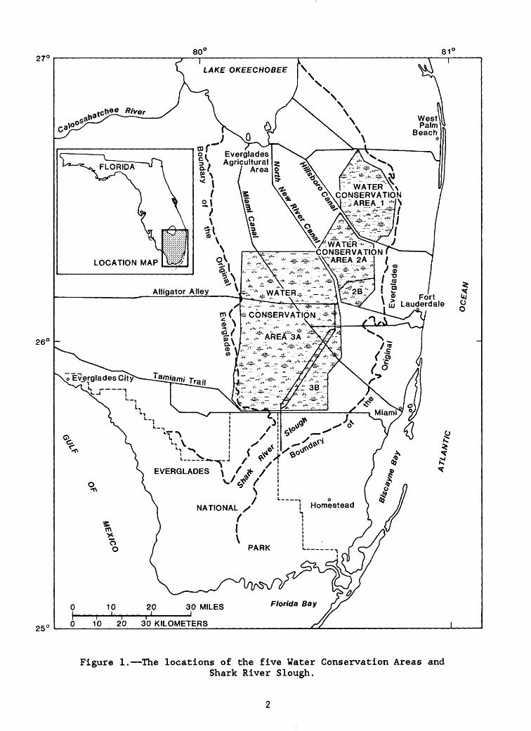
The historical Everglades extended from Lake Okeechobee south to the Gulf of Mexico prior to drainage methods introduced by man in the 20th century. During the wet season, from May through October, water flowed in a large sheet through this predominantly sawgrass marsh to the Gulf of Mexico. A major part of this historical marsh is currently (1987) delineated by five Water Conser­ vation Areas, which are shallow wetlands enclosed by levees during the 1950' s and 1960 's for water -management purposes. The largest, Water Conservation Area 3A (WCA— 3A) , releases water into the major undisturbed part of The Ever­ glades, the Shark River Slough, within Everglades National Park (fig. 1).

The schedule for releasing water and the quantity of water released to the park have undergone several changes. From 1970 to 1983, deliveries to Shark River Slough were managed by the South Florida Water Management District according to water-level regulation schedules set by the U.S. Army Corps of

•U.S. Geological Survey. 2 National Park Service.oSouth Florida Water Management District.

27<

26

25 C

LAKE OKEECHOBEE

WestPalm

Beach

Everglades Agricultural

Area

WATER \ CONSERVATION

AREA

WATER - - CONSERVATION

LOCATION MAP

Alligator AlleyFort

LauderdaleI* CONSERVATION ;*

oEverglades Cit

EVERGLADES

30 KILOMETERS

o _

Figure 1.—The locations of the five Water Conservation Areas andShark River Slough.

Engineers and a minimum monthly surface-water delivery schedule mandated by the U.S. Congress in 1970 (Public Law 91-282). Concurrently, Senate Report No. 91-895 charged the U.S. Army Corps of Engineers and the National Park Service with establishing water-quality requirements for maintaining the environment of the Everglades National Park. The water-quality standards for the released water were based on an upper control chart limit that reflected the true mean concentration, standard deviation, and sampling frequency (Rosendahl and Rose, 1979) for samples collected between 1970 and 1978 at S-12C and L—67A. The true mean is calculated from the arithmetic mean with an assumption of a normal concentration distribution (Bowker and Liberman, 1972). In 1979, the U.S. Army Corps of Engineers began water-quality monitoring near three inflow structures to the Everglades National Park to assure that water of acceptable quality was being delivered to the park. Water-quality informa­ tion at five inflow structures that supply WCA-3A were not part of the formal agreement but were included in the U.S. Army Corps of Engineers' monitoring program.

Concentrations of water-quality constituents could be below the standards established in 1979 but show an upward concentration trend that would indicate a probable future exceedance. Recognition of constituent trend increases would be useful in identifying sources and proposing mitigation solutions prior to significant ecological damage. In an attempt to evaluate any statis­ tically significant time trends in water quality, the National Park Service and the U.S. Geological Survey evaluated the water-quality data base used by the U.S. Army Corps of Engineers. Because of the data-collection frequency of four times per year, the U.S. Army Corps of Engineers and Everglades National Park agreed that evaluation of a semimonthly data set used by the South Florida Water Management District would be more appropriate for testing the application of trend analysis to water quality. Equally important to the trend evaluation were the existence of discharge and rainfall data bases stored in the computer by South Florida Water Management District.

Purpose and Scope

The purpose of this report is to present a description of the methods and results of a time-trend analysis of water-quality data from 10 water flow structures around WCA-3A (fig. 2). Another purpose is to consider the appli­ cability of this type of trend analysis to the current monitoring program as defined by the 1979 Memorandum of Agreement between the National Park Service, South Florida Water Management District, and the U.S. Army Corps of Engineers (Supplementary Data I). The test for trend used in this analysis is the Seasonal Kendall test (Hirsch and others, 1982). Specific conductance (COND) and concentrations of orthophosphate (P04 ), nitrate-nitrogen (N03 ), total Kjeldahl nitrogen (TKN) , and total nitrogen (TN) were tested for trends over the 5-year period 1978 through 1982. Many of the 10 flow structures tested had 24 samples per year.

The time-trend analysis included regression models that relate water- quality constituents and antecedent rainfall history for the 10 flow struc­ tures. Where the r-squared value indicated a regression relation representing greater than 5 percent of the concentration variation, the model residuals were tested for trend. Relations between antecedent discharge history and water-quality constituents also were defined by multiple regression models. Residuals from discharge-based regression models were not evaluated for trend because of flow control changes within the 5-year period.

EVERGLADES AGRICULTURAL AREA

S-6

\Lr3S-8

BIG CYPRESS BASIN

Park

EASTERNURBAN

COASTALZONE

EVERGLADES NATIONAL PARK

EXPLANATION

S-9 INFLOW STRUCTURE • AND NUMBER

O, PERCENT OF TOTAL V INFLOW , 1978

S-I5I OUTFLOW STRUCTURE D AND NUMBER

£L PERCENT OF TOTAL V OUTFLOW, 1978

024 MILESh-V-J024 KILOMETERS

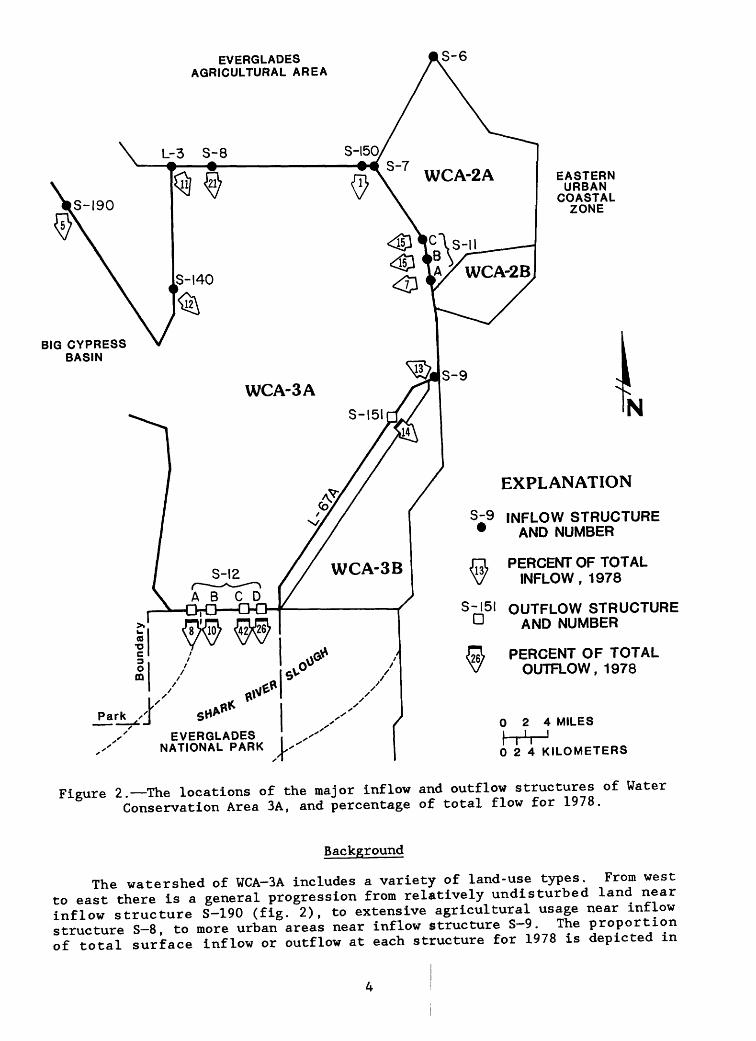
Figure 2.—The locations of the major inflow and outflow structures of Water Conservation Area 3A, and percentage of total flow for 1978.

Background

The watershed of WCA-3A includes a variety of land-use types. From west to east there is a general progression from relatively undisturbed land near inflow structure S-190 (fig. 2), to extensive agricultural usage near inflow structure S-8, to more urban areas near inflow structure S-9. The proportion of total surface inflow or outflow at each structure for 1978 is depicted in

figure 2, but the actual discharge is seasonal and varies annually on the basis of management decisions and rainfall. Total minimum discharge (260,000 acre-feet per year) through the four S—12 outflow gates on the south end of WCA—3A was guaranteed by congressional mandate (Public Law 91—282) until 1983, but could vary considerably among the four S—12 gates. South Florida Water Management District records for 1978 indicate the following inflow and outflow from WCA—3A, in acre-feet.

Inflow Outflow (in acre-feet)____ _____(in acre-feet)_______

S-8 260,163 S-151 90,543S-9 157,719 S-12A 54,590S-140 147,381 S-12B 64,714S-150 14,281 S-12C 271,878S-190 66,451 S-12D 168,807L-3 140,677 Outflow 650,532S-11A 86,364 Evapotrans- 2,169,360S-11B 188,766 pirationS-11C 180,322 Total out 2,819,892

Inflow 1,242,124Rainfall 1,629,749Total in 2,871,873

The largest source of inflow to WCA—3A is rainfall (approximately 50 to 80 percent), and the largest source of outflow for the 786-square-mile marsh is evapotranspiration (approximately 70 percent, or 2 million acre-feet). The mean residence time of water is 0.81 year for the shallow (ranging from dry to 2 feet, 6 inches) marsh. Because of the physical characteristics of WCA—3A, nitrogen and phosphorus are readily incorporated into marsh vegetation and are largely retained in the conservation area (74 and 96 percent, respectively) (Federico and others, in press).

The rainfall pattern over Water Conservation Area 3A varies seasonally with a 44.27-inch per year, 30-year moving average for the period 1952 through 1981 (Lin and others, 1984). The rainfall for the years 1978 through 1982 was 88, 83, 95, 106, and 121 percent of normal, respectively. This generally increasing rainfall component of the total inflow may affect water-quality concentration by dilution or by acting as a source for specific constituents.

The general annual rainfall pattern is highly seasonal with numerous examples of seasonal effects on concentration (Waller and Earle, 1975). Water-quality concentrations are serially dependent and the Seasonal Kendall test for trend was chosen in an attempt to employ a statistical technique that eliminates the effects of serial correlation.

An implicit assumption in the overall analysis is that the probability distribution of rainfall or discharge is unchanged through the 5-year evalua­ tion period. A conscious change in flow causes predicted values early or late in an evaluation period to be consistently higher or lower than observed values. Any water-quality model constructed as a function of discharge may inadvertently produce an apparent trend that is a result of flow control. The regression model produces a set of concentration residuals generally higher or lower than warranted; this causes an apparent trend because of the change in water management. In 1983, the National Park Service, the U.S. Army Corps of Engineers, and the South Florida Water Management District agreed to a con­ tinuous flow policy for water entering Shark River Slough. This anticipated

policy change is reflected in figure 3, which is a plot of the 30-day cumula­ tive rainfall and discharge at outflow structure S-12A for the 1978-82 evalua­ tion period. The last 6 months of 1982 show a definite increase of discharge over rainfall compared to previous years. Other examples of discharge pattern shifts appear throughout the period of record at all 10 flow structures. Therefore, regression models based on discharge, although constructed, were not considered in determining trends in model residuals.

170,

160,000

140,000

O

120,000

OCOD^f 100,000

LU O QC

IO 80,000

Q LU

60,000

40,000

20,000

I I I I I I I I I I I I I I I I I I I I I

O RAINFALL

• DISCHARGE

000000°

•0000000°kO

ill i i i i i i i i i i i i i i i i i i

- 250

LU

H200 J

150

- 100 >

-50 g

1978 1979 1980 1981 1982

Figure 3.—Thirty-day cumulative discharge and rainfall at structure S-12A.

DATA PROCESSING AND ANALYSIS

Parts of three data sets (water quality, discharge, and rainfall) were retrieved from the South Florida Water Management District computer onto a magnetic tape and loaded onto a U.S. Geological Survey PRIME 1 computer located In Tampa, Fla. These data sets were edited and transferred to the Amdahl computer in Reston, Va., which had a Statistical Analysis System (SAS) library. Additional editing, merging, model construction, and trend analyses were performed with SAS format routines run In batch mode from the Tampa PRIME. Figure 4 summarizes the major steps In reformatting the South Florida Water Management District data sets and for performing the statistical analyses.

Water-Quality Data

The water-quality data set (WCAQW) contained 22,242 card images repre­ senting 3,707 water-quality analyses, from the 10 flow structures, for the period 1978 through 1982. Each analysis was represented by the six-card format listed In Supplementary Data II. A sample code type was included on card six and provided the main mechanism for deleting samples that were related to quality assurance (replicates) and special collection techniques (flow-weighted sampling, bottom samples, and others). The number of samples retained for analysis at the 10 flow structures from the WCAQW water-quality set are listed In table 1. Inflow structures S—150, S—11A and C, and outflow structures S—12B and C were excluded from the analyses. Entries into the computer for samples that were collected twice monthly by standard grab-sample methods were retained for transfer to the Amdahl computer In Reston, Va. The program transferring the edited data files is termed IEBGENER (fig. 4).

Discharge Data Base

Dally discharge, In cubic feet per second, for the 10 flow structures was represented by 1,810 card Images that had three cards per month. The day of the month was Implicit In the column of the card. An example of the format is shown In Supplementary Data II. The 5-year period at a structure would be represented by 180 card Images. Each file was reviewed for missing and dupli­ cate records, corrected, and then transferred to an Amdahl computer In Reston, Va. A program was used to reassemble a discharge data file (for example, QS7 In fig. 4) that contained an explicit date. A listing of this program (TRANSPOSE) Is given In Supplementary Data III.

Rainfall Data Base

The South Florida Water Management District rainfall data files employed the same format of three cards per month, Implicit day, format used for the discharge data files. The 33 rainfall collection stations In the proximity of the 10 flow structures are shown In figure 5. All records had some missing data for the 5-year period. Table 2 lists the 10 flow structures and Identi­ fies the rainfall stations that are most representative of each structure. Parts of adjacent rainfall records were spliced into the primary rainfall station records to complete a continuous record at each rainfall station near the 10 flow structures. Imbedded in the rainfall records were seven alpha remark codes that Indicated missing or accumulated rainfall data. After editing, the remark codes were deleted, and the file transferred to the Amdahl and TRANSPOSED (fig. 4).

Use of brand, firm, or trade names in this report is for identification purposes only and does not constitute endorsement by the U.S. Geological Survey.

I———————SFWMD DATA (supplementary data II)———iRAINFALL (RF) DISCHARGE (Q) WATER QUALITY (QW)

|1 3 cards 1

i — -LOAD

Ll 3 cardsl LU[[

DDlftAC? frfllYIC - ———

6 cards] 1

LOAD

LJpLJ |LOAD

DATAJ (Q_DATA)

SEPARATE I

spliceSEPARATE SEPARATE

180 lines

(RFQS)

El

missiiiy record

—— 1180 lines

(o|7)

DIT-*- B.F.etc.

180 lines

CRFQS)— ——

DELETE: duplicates nonsurface

RETAIN: surface wa

3432 lines

(QWST)576 analyses

•*— EDIT

ter I

528 lines

(QWST)88 analyses

———— | ———

( IEBGENER (transfer)

———— AMDAHL

^TRANSPOSE (supplementary data III))

ZHT ^TTRF95 ) (QS7

n

< MERGE (supplementary data IV)

(MERGED S7 DATAJ up o

_______>^ *^<£_______ j

(MAX R) (supplementary data V) (MAX R)

— — —— —— — _

TABLE 5MODEL

SELECTION

— — —— .

TABLE 6

— ——— n

L.

GENERALIZED LINEAR MODEL/TREND ____(supplementary data VI)____

(SEASONAL KENDALT)» zn

CONCENTRATIONONLY

(table 7)

Figure 4.—Schematic diagram of major data-processing steps in thetime-trend analysis.

Table 1.—Sample collection location descriptions,, total number of water-quality samples, and number suitable for trend analysis

[SFWMD - South Florida Water Management District]

Samplecollectionlocation(flow

structure)

Total number

of samples in SFWMD data base

Number of samples suitable for trend analysis

Sample collection location description

S-190

L-3

S-8

S-140

S-7

S-11B

S-9

S-151

S-12D

S-12A

375

97

124

418

571

124

502

326

376

309

89 Discharge from S-190 in C-28 canal under State Road 84 bridge.

85 L—3 canal near the Deer Fence Canal bridge.

62 S-8 structure pumps water from theEverglades agricultural area into the Miami Canal. Upstream sample site.

101 S-140 pumping station near State Road 84. Upstream sample site.

88 S-7 pump station along State Road 27 that discharges to WCA—2A. Upstream sample site.

62 Gate structure on U.S. Highway 27 that releases water from WCA-2A to WCA-3A. Upstream sample^site.

108 S-9 pumps water into WCA-3A near U.S. Highway 27. Upstream sample site.

96 Gate structure on the Miami Canal that releases water from WCA—3A to WCA-3B. Upstream sample site.

116 Easternmost S-12 gate structure at U.S. Highway 41 that releases water from WCA-3A into the Shark River Slough. Upstream sample site.

90 Westernmost S-12 gate at U.S. Highway 41structure that releases water from WCA—3A into marshes and prairies of Everglades

________National Park. Upstream sample site._____

Constituent Selection and Merging of Data Files

The water-quality, discharge, and rainfall data files were stored on the Amdahl. The water-quality file contained 37 constituents in the format shown in Supplementary Data II. The five constituents (COND, P04 , N03 , TKN, and TN) were selected from statistical summaries of 37 constituents at the 10 flow structures. The South Florida Water Management District and Everglades National Park selected these five as being representative of many other con­ stituents or having particular ecological significance. Specific conductance

was selected because it integrates all the dissolved charged chemical constit­ uents . Previous work (Flora and Rosendahl, 1981) has shown significant rela­ tions between specific conductance and most of the major cations and anions in water in The Everglades. Specific conductance also may be used as an indi­ cator of the origin of water (that is, canal, marsh, or precipitation). Nitrogen and phosphorus are important to the types of plant growth in the marsh ecosystem (Swift, 1981). The general pattern of specific conductance, orthophosphate, and nitrate can be seen in figures 6 through 8, which show the 5-year mean concentrations at the 10 flow structures. Elevated concentrations of nitrogen and phosphorus and elevated specific conductance are related to agricultural activities in the Everglades Agricultural Area (fig. 2).

Table 2.—Ten flow structures and most representative rainfall-collection stations

Rainfall-Flow collection

structure______________________station

S-190 RF145L-3 RF182S-8 RF98S-140 RF145S-7 RF99

S-11B RF106 S-9 RF115 S-151 RF115 S-12D RF6054 S-12A_________________________RF6054

Water quality, discharge, and rainfall were merged into a single SAS data set (for example, MS7 in fig. 4) on the basis of water-quality sample date. An important feature of the MERGE program is the creation of three antecedent conditions for discharge and rainfall. The MERGE program is listed in Supple­ mentary Data IV. The three cumulative antecedent periods chosen were for 7, 14, and 30 days prior to the sample date.

Model Selection with Stepwise Regression

The cumulative antecedent discharge or rainfall are the independent variables used to construct regression models for the water-quality dependent variables. Both the independent and the dependent variables can be trans­ formed into a variety of complex functions. The simplest relation is linear concentration versus linear independent variable. Table 3 shows the matrix of simple relations tested.

Table 3.—Combinations of mathematical transformations usedin model construction

Water-quality Independent variables constituent ____(rainfall and discharge)

form

Linear Log

Linear

X X

Inverse

X X

Log

X X

Quadratic

X

10

RF76 RF220

A

ALLIGATOR ALLEY

CYPRESS

EXPLANATION

INFLOW STRUCTURE

OUTFLOW STRUCTURE

DAILY RAINFALL RECORDING GAGE

PERIODIC RAINFALL GAGE

GULF?OF

MEXICO^ 10 KILOMETERS

Figure 5.—The locations of the 33 rainfall collection stations nearWater Conservation Area 3A.

11

EVERGLADES AGRICULTURAL AREA

S-6

\

555

EASTERNURBANCOASTALZONE

EVERGLADES NATIONAL PARK

EXPLANATION

S-9 INFLOW STRUCTURE • AND NUMBER

S-I5I OUTFLOW STRUCTURE D AND NUMBER

674 MEAN SPECIFICCONDUCTANCE, IN MICROSIEMENS PER CENTIMETER 1978-82

024 MILEShrVJ024 KILOMETERS

Figure 6.—Mean specific conductance at the 10 flow structures

12

EVERGLADES AGRICULTURAL AREA

S-6

\

BIG CYPRESS BASIN

_ParJL^;jX s****EVERGLADES

NATIONAL PARK

EASTERNURBANCOASTALZONE

I '

N

EXPLANATION

S-9 INFLOW STRUCTURE • AND NUMBER

S-I5I OUTFLOW STRUCTURE a AND NUMBER

3 MEAN ORTHOPHOSPHATE CONCENTRATION, IN MICROGRAMS PER LITER, 1978-82

024 MILESh-^H024 KILOMETERS

Figure 7.—Mean orthophosphate concentration at the 10 flow structures

13

EVERGLADES AGRICULTURAL AREA

S-6

\

BIG CYPRESS BASIN

EASTERNURBAN

COASTALZONE

EVERGLADES NATIONAL PARK

N

EXPLANATION

S-9 INFLOW STRUCTURE ' AND NUMBER

S-I5I OUTFLOW STRUCTURE u AND NUMBER

100 MEAN NITRATECONCENTRATION, IN MICROGRAMS PER LITER, 1978-1982

024 MILESKV-J024 KILOMETERS

Figure 8.—Mean nitrate concentration at the 10 flow structures

14

The linear equation for orthophosphate-phosphorus (P0 4 ) at inflow struc­ ture L—3 would have the form:

(P04 ) - 0.0222(RF30T) - 0.034 (1)

where:

(P0 4 ) is orthophosphate-phosphorus concentration, in milligrams per liter,

(P0 4 ) > 0.004 (the detection limit), and

RF30T is antecedent 30-day cumulative rainfall, in inches.

The equation, for example, would predict a concentration of 0.188 mg/L (milligrams per liter) for 10 inches of rainfall in the previous 30 days (RF30T - 10). The relation had an r-squared value of 0.63, which means that 63 percent of the observed P0 4 concentration variation is explained by this simple relation between 30-day antecedent rainfall and orthophosphate concen­ tration. Each water-quality constituent at each structure had both a linear and log-transformed concentration regression model that had three or more forms of the independent rainfall and discharge variables (table 3). The water-quality constituent model for a particular site was the best single relation from 42 variations of concentration, rainfall, or discharge transfor­ mations. There are 50 final models representing the best stepwise regression model selected for each of the five water-quality constituents at each of the 10 flow structures.

An example of the type of stepwise regression program that was used to 'select the best independent variable (MAXR) is listed in Supplementary Data V. The approach is to allow the best single variable with the maximum r-squared value to be selected from the available independent variables.

Model Output with General Linear Models

The SAS stepwise model construction (MAXR) was used to find the single best independent variable. When this variable is defined, model construction is repeated with GLM (GLM is the SAS acronym for General Linear Models (Helwig and Council, 1979)) using only the best independent variable. The GLM program contains provisions for retaining predicted and residual values as output (Supplementary Data VI). A residual is the difference between the observed concentration and the concentration predicted by the model. In each case, a graph of residuals versus predicted concentrations was plotted to eliminate model output that had obvious patterns. Three major patterns in the residuals plot may occur (Daniel and Wood, 1971):

1. Pronounced departure of the residuals related to the size of the predicted value; this is usually wedge shaped.

2. A U-shaped pattern that indicates a curvilinear model relation would produce a better representation of the data.

3. A plot that indicates clustering of predicted values; high or low values (outliers) offset from the cluster may have an unwarranted effect on the slope of predictive equation.

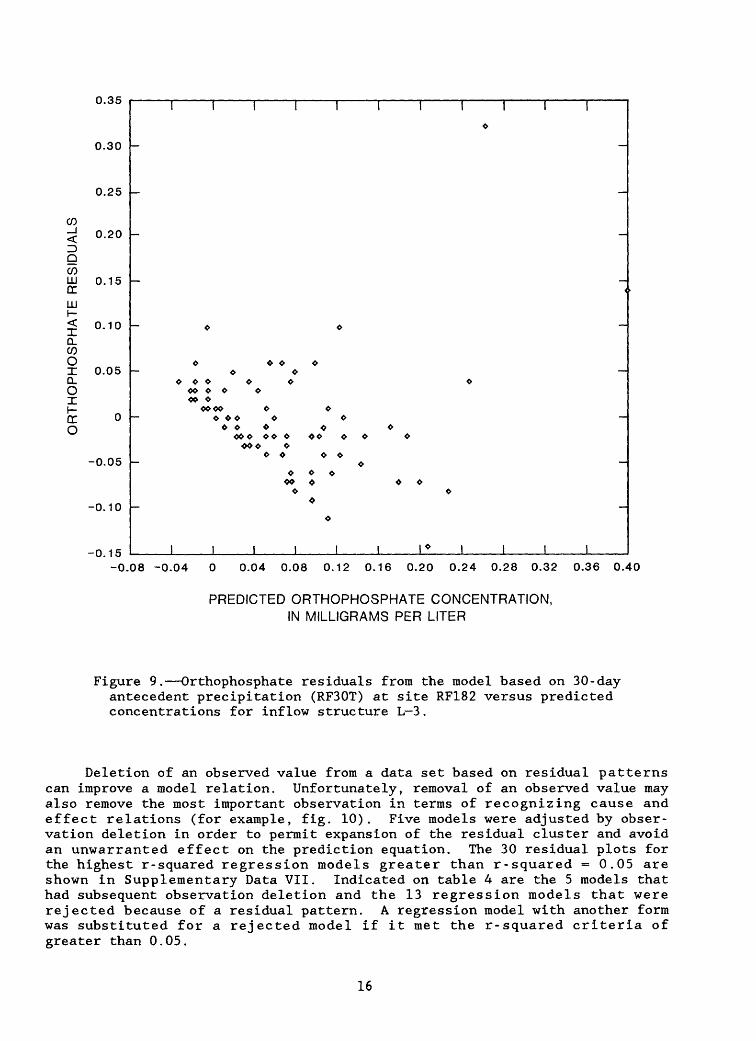
Figure 9 is a plot of P0 4 residuals from the model based on RF30T versuspredicted concentrations for structure L—3, whereas figure 10 is a plot of P0 4residuals from the Log (P04 ) - 0.001 (RSQ30) + 0.016 regression model.

15

CO_l<=>QCO LLJocLJJ

X Q. COoCL OIh- oc o

0.35

0.30

0.25

0.20

0.15

0.10

0.05

-0.05

-0.10

-0.15

<x> o o

ooo oo oo

o o

o o

J____I____I

-0.08 -0.04 0 0.04 0.08 0.12 0.16 0.20 0.24 0.28 0.32 0.36 0.40

PREDICTED ORTHOPHOSPHATE CONCENTRATION, IN MILLIGRAMS PER LITER

Figure 9.—Orthophosphate residuals from the model based on 30-day antecedent precipitation (RF30T) at site RF182 versus predicted concentrations for inflow structure L—3.

Deletion of an observed value from a data set based on residual patterns can improve a model relation. Unfortunately, removal of an observed value may also remove the most important observation in terms of recognizing cause and effect relations (for example, fig. 10). Five models were adjusted by obser­ vation deletion in order to permit expansion of the residual cluster and avoid an unwarranted effect on the prediction equation. The 30 residual plots for the highest r-squared regression models greater than r-squared = 0.05 are shown in Supplementary Data VII. Indicated on table 4 are the 5 models that had subsequent observation deletion and the 13 regression models that were rejected because of a residual pattern. A regression model with another form was substituted for a rejected model if it met the r-squared criteria of greater than 0.05.

16

CO

D QCOLUocLU

X Q. CO O I Q. O XI- oc O

0.30

0.25

0.20

0.15

0.10

0.05

-0.05

-0.10

-0.15

-0.20

o o o o

oo

00 O *- o oo0000 00 O Ooooooo o

o o o o o

0 0.05 0.10 0.15 0.20 0.25 0.30 0.35 0.40 0.45 0.50 0.55 0.60 0.65

PREDICTED ORTHOPHOSPHATE CONCENTRATION, IN MILLIGRAMS PER LITER

Figure 10.—Orthophosphate residuals from the quadratic model based on the square of 30-day antecedent precipitation (RSQ30) at site RF 182 versus predicted concentrations for inflow structure L-3.

Seasonal Kendall Test

The second major feature of GLM residuals is to permit output directly into the Seasonal Kendall test (Hirsch and others, 1982). Observed concentra­ tions for 50 structure-constituent combinations and 29 model residuals were tested for time trend.

17

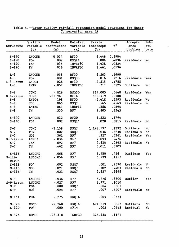
Table 4.—Water quality-rainfall regression model equations for WaterConservation Area 3A

Structure

S-190S-190S-190S-190

L-3L-3

L-3 -Re runL-3

S-8S-8-Rerun

S-8S-8S-8S-8

S-140S-140

S-7S-7S-7

S-7 -Re runS-7S-7

S-11BS-11B-RerunS-11BS-11BS-11B

S-9S-9-Rerun

S-9S-9

S-151

S-12DS-12D

Quality variable

(y)

LNCONDP04TKNTN

LNCONDP04LNP04LNTN

CONDCONDLNP04N03LNTKNTN

LNCONDP04

CONDP04N03LNN03TKNTN

LNCONDLNCOND

P04N03TN

LNCONDLNCONDP04N03

P04

CONDP04

Model coefficient

(m)

-0.034.002.035.036

-.058.001.028

-.052

-.826-21.94

.198

.065

.061

.530

-.032.002

-3.139.002.361

-.034.092.462

-.068-.056

.002

.021

.021

-.034-.027.000.025

9.275

-2.260.000

Rainfall variable

(x)

RF30RSQ14INVRF30INVRF30

RF30RSQ30RF30INVRF30

RSQ30RF14RF30RSQ7LNRF14RF7

RF30RSQ14

RSQ7RSQ7RF7RF7RF7RF7

RF7RF7

RSQ7RSQ7RSQ7

RF7RF7RSQ7RF7

RSQ14

RSQ14RF14

Y-axis intercept

(b)

6.446.004

1.4381.461

6.263.016

-4.815.711

869.003886.519-5.418

.565

.8882.803

6.232.020

1,198.537.034.327

7.0932.6353.011

6.9506.939

.001

.1022.627

6.7766.771.004.007

.005

691.819.003

r2

0.3904.4836.0534.0536

.5690

.7216

.4758

.0525

.0648

.0588

.3593

.4563

.0894

.3545

.3794

.3815

.1332

.6230

.5361

.2476

.0593

.3703

.456

.1157

.9570

.7403

.3698

.3600

.1010

.8801

.5407

.0573

.0887

.0543

Accept­ ance

problem

Residuals

Residuals

Outliers

Residuals

ResidualsResiduals

Residuals

OutliersResidualsResiduals

Residuals

Outliers

ResidualsResiduals

Outlier

Residuals

OutliersResidual

Sub­ sti­ tute

No

Yes

No

Yes

NoNo

No

NoNoYes

No

Yes

NoNo

Yes

No

NoNo

S-12A COND -23.318 LNRF30 326.)34 .1121

18

The Seasonal Kendall test is a nonparametric trend test based on Kendall's Tau test (Kendall, 1975). The seasonal provision permits comparison of data pairs from the same season (Supplementary Data VI). Season - 6 causes the median concentration from January and February 1978 to be compared (higher or lower) with January and February 1979. Other season — 6 time periods are March—April, May—June, July—August, September-October, and November—December. Adjacent time periods (pairs, for example, 1978—79, 1979—80, and so forth) are compared, and the number of intervals (nvals) would be 24 for a 5-year time span with 1 or more concentrations recorded for each 2-month segment. An increase between a pair is recorded as a plus (concordant) and a decrease as a minus (discordant) . The differences between the plus and minus pairs are tested for significance (p-level). The Seasonal Kendall test has an addi­ tional provision to calculate a slope based on the statistical distribution of the concordant pairs (Hirsh and others, 1982).

RESULTS

Evaluation with Rainfall and Discharge Stepwise Models

The initial model construction phase permitted a choice of three rainfall and three discharge independent variables. The linear, log, and inverse functions listed in table 3 were evaluated. The initial stepwise analysis of water quality included discharge as an independent variable, and the results are presented in table 5. Discharge entered the stepwise regression in 13 cases of 50 possible constituent-structure cases. Rainfall had the highest r-squared for 24 cases. The remaining 13 cases lacked significance; they had an r-squared less than 0.05.

Evaluation with Rainfall Stepwise Model

With the elimination of discharge as a possible independent variable, MAXR was revised to simultaneously evaluate linear, log, and inverse forms of rainfall history. An additional modification was the program statement set­ ting all P0 4 concentrations less than 0.004 to 0.004 mg/L. The reported detection limit for P0 4 was raised from 0.002 to 0.004 during the study period. This reporting change of the higher detection limit resulted in apparent significant P0 4 -trend increases at several structures. Supplementary Data V lists the SAS program used for evaluating the linear and log concentra­ tion versus the three transformations of antecedent cumulative rainfall (linear, log, and inverse).

An additional set of rainfall transformations was entertained with a simple quadratic model: RSQ30 - RF30T x RF30T. The r-squared comparison of the three evaluations is listed in table 6. The addition of the quadratic rainfall, independent variable, resulted in 14 models with a greater r-squared value than the other 6 independent rainfall variable forms evaluated by linear and log concentrations. An arbitrary level of 0.05 for r-squared was used as the lower limit for an acceptable concentration-rainfall model. Using this criteria, 20 of 50 water-quality-structure combinations had r-squared values less 0.05. This means that 20 water-quality-structure combinations failed to show a relation with 21 possible antecedent rainfall model choices (table 3).

19

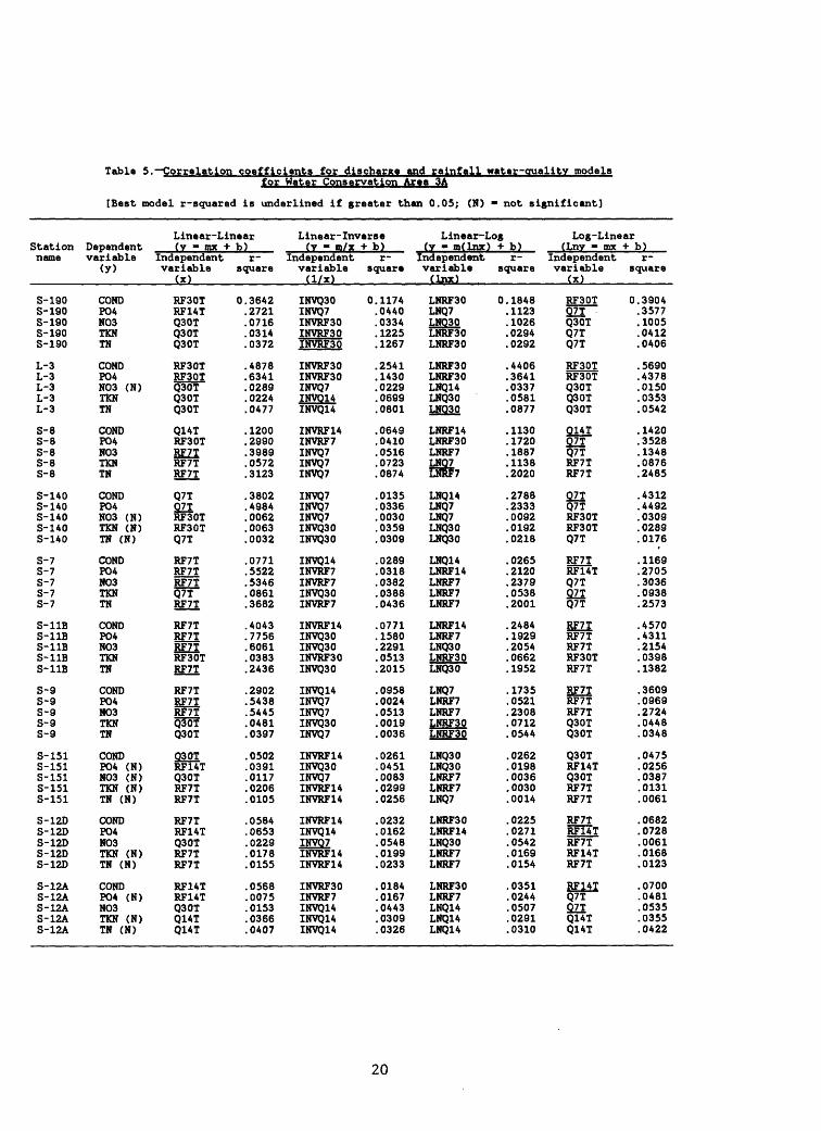
Table 5."Correlation coefficients for discharge and rainfall water-quality modelsfor Water Conservation Area 3A

[Best model r-squared is underlined if greater than 0.05; (N) m not significant]

Linear-LinearStationname

S-190S-190S-190S-190S-190

L-3L-3L-3L-3L-3

S-8S-8S-8S-8S-8

S-140S-140S-140S-140S-140

S-7S-7S-7S-7S-7

S-11BS-11BS-11BS-11BS-11B

S-9S-9S-9S-9S-9

S-151S-151S-151S-151S-151

S-12DS-12DS-12DS-12DS-12D

S-12AS-12AS-12AS-12AS-12A

Dependentvariable

(y)

CONDP04N03TKNTN

CONDP04N03 (N)TKNTN

CONDP04N03TKNTN

CONDP04N03 (N)TKN (N)TN (N)

CONDP04N03TKNTN

CONDP04N03TKNTN

CONDP04N03TKNTN

CONDP04 (N)N03 (N)TKN (N)TN (N)

CONDPO4N03TKN (N)TN (N)

CONDPO4 (N)N03TKN (N)TN (N)

(y - mx +Independentvariable

(x)

RF30TRF14TQ30TQ30TQ30T

RF30TRF30TQ30TQ30TQ30T

Q14TRF30TRF7TRF7TRF7T

Q7T2ZIRF30TRF30TQ7T

RF7TRF7TRF7TQ7TRF7T

RF7TRF7TRF7TRF30TRF7T

RF7TRF7TRF7TQ30TQ30T

Q30TRF14TQ30TRF7TRF7T

RF7TRF14TQ30TRF7TRF7T

RF14TRF14TQ30TQ14TQ14T

b)r~

square

0.3642.2721.0716.0314.0372

.4878

.6341

.0289

.0224

.0477

.1200

.2990

.3989

.0572

.3123

.3802

.4984

.0062

.0063

.0032

.0771

.5522

.5346

.0861

.3682

.4043

.7756

.6061

.0383

.2436

.2902

.5438

.5445

.0481

.0397

.0502

.0391

.0117

.0206

.0105

.0584

.0653

.0229

.0178

.0155

.0568

.0075

.0153

.0366

.0407

Linear-Inverse(y - m/x

Independentvariable(1/x)

INVQ30INVQ7INVRF30INVRF30INVRF30

INVRF30INVRF30INVQ7INVQ14INVQ14

INVRF14INVRF7INVQ7INVQ7INVQ7

INVQ7INVQ7INVQ7INVQ30INVQ30

INVQ14INVRF7INVRF7INVQ30INVRF7

INVRF14INVQ30INVQ30INVRF30INVQ30

INVQ14INVQ7INVQ7INVQ30INVQ7

INVRF14INVQ30INVQ7INVRF14INVRF14

INVRF14INVQ14INVQ7INVRF14INVRF14

INVRF30INVRF7INVQ14INVQ14INVQ14

+ b)r-

square

0.1174.0440.0334.1225.1267

.2541

.1430

.0229

.0699

.0801

.0649

.0410

.0516

.0723

.0874

.0135

.0336

.0030

.0359

.0309

.0289

.0318

.0382

.0388

.0436

.0771

.1580

.2291

.0513

.2015

.0958

.0024

.0513

.0019

.0036

.0261

.0451

.0083

.0299

.0256

.0232

.0162

.0548

.0199

.0233

.0184

.0167

.0443

.0309

.0326

Linear-Log(y - m(ln)

Independentvariable(Lnx)

LNRF30LNQ7LNQ30LNRF30LNRF30

LNRF30LNRF30LNQ14LNQ30LNQ30

LNRF14LNRF30LNRF7LNQ7LNRF7

LNQ14LNQ7LNQ7LNQ30LNQ30

LNQ14LNRF14LNRF7LNRF7LNRF7

LNRF14LNRF7LNQ30LNRF30LNQ30

LNQ7LNRF7LNRF7LNRF30LNRF30

LNQ30LNQ30LNRF7LNRF7LNQ7

LNRF30LNRF14LNQ30LNRF7LNRF7

LNRF30LNRF7LNQ14LNQ14LNQ14

x) + b)t r-

square

0.1848.1123.1026.0294.0292

.4406

.3641

.0337

.0581

.0877

.1130

.1720

.1887

.1138

.2020

.2788

.2333

.0092

.0192

.0218

.0265

.2120

.2379

.0538

.2001

.2484

.1929

.2054

.0662

.1952

.1735

.0521

.2308

.0712

.0544

.0262

.0198

.0036

.0030

.0014

.0225

.0271

.0542

.0169

.0154

.0351

.0244

.0507

.0291

.0310

Log-Linear(Lny « mx

Independentvariable

(x)

RF30T221""Q30TQ7TQ7T

RF30TRF30TQ30TQ30TQ30T

Q14TQ7TQ7TRF7TRF7T

221Q7TRF30TRF30TQ7T

RF7TRF14TQ7T221Q7T

RF7TRF7TRF7TRF30TRF7T

RF7TRF7TRF7TQ30TQ30T

Q30TRF14TQ30TRF7TRF7T

RF7TRF14TRF7TRF14TRF7T

RF14TQ7T221Q14TQ14T

+ b)r-

square

0.3904.3577.1005.0412.0406

.5690

.4378

.0150

.0353

.0542

.1420

.3528

.1348

.0876

.2485

.4312

.4492

.0309

.0289

.0176

.1169

.2705

.3036

.0938

.2573

.4570

.4311

.2154

.0398

.1382

.3609

.0969

.2724

.0448

.0348

.0475

.0256

.0387

.0131

.0061

.0682

.0728

.0061

.0168

.0123

.0700

.0481

.0535

.0355

.0422

20

Table 6.~~Correlation coefficients for rainfall water-quality regressionmodels for Water Conservation Area 3A

[Best model r-squared is underlined if greater than 0.05; (N) = not significant]

Structure

S-190S-190S-190S-190S-190

L-3L-3L-3L-3L-3

S-8S-8S-8S-8S-8

S-140S-140S-140S-140S-140

S-7S-7 S-7S-7S-7

S-11BS-11BS-11BS-11BS-11B

S-9S-9S-9S-9S-9

S-151S-151S-151S-151S-151

S-12DS-12DS-12DS-12DS-12D

S-12AS-12AS-12AS-12AS-12A

Variable

CONDP04N03 (N)TKNTN

CONDP04N03 (N)TKN (N)TN

CONDP04N03TKNTN

CONDP04N03 (N)TKN (N)TN (N)

CONDP04 N03TKNTN

CONDP04N03TKN (N)TN

CONDP04N03TKN (N)TN (N)

COND (N)P04N03 (N)TKN (N)TN (N)

CONDP04N03 (N)TKN (N)TN (N)

CONDP04 (N)N03 (N)TKN (N)TN (N)

Linear(v - m(x)

RF30T 0RF14TRF7TINVRF30INVRF30

RF30TRF30TRF7TINVRF30INVRF30

RF14TRF30TRF7TRF7TRF7T

RF30TRF30TRF30TRF30TINVRF7

RF7TRF7T RF7TRF7TRF7T

RF7TRF7TRF7TRF30TRF7T

RF7TRF7TRF7TRF30TRF30T

INVRF30RF14TLNRF7RF7TINVRF30

RF7TRF14TLNRF14INVRF14INVRF14

LNRF30RF14TLNRF14RF30TRF30T

r2

+ b)

.3642

.2722

.0073

.0534

.0536

.4878

.6335

.0148

.0242

.0252

.0588

.2972

.3990

.0573

.3124

.3341

.3103

.0062

.0063

.0014

.0773

.5536

.5346

.0569

.3681

.4042

.7773

.6063

.0384

.2436

.2901

.5779

.5446

.0270

.0145

.0191

.0402

.0177

.0206

.0205

.0585

.0543

.0191

.0202

.0269

.1121

.0101

.0328

.0289

.0319

LOR(Iny - m(x)

RF30T 0.RF30TLNRF7INVRF7INVRF14

RF30TRF30TINVRF30INVRF30INVRF30

RF14TRF30TRF14TLNRF14RF7T

RF30TRF30TLNRF30RF30TRF30T

RF7TRF14T RF14TRF7TRF7T

RF7TRFTfRF7TRF30TRF7T

RF7TRF7TRF7TRF30TLNRF30

INVRF30RF14TINVRF7INVRF30INVRF30

RF7TRF14TLNRF7INVRF14INVRF14

LNRF30RF14TLNRF14RF30TRF30T

r2

+ b)

39042513012603030293

56904758015704710525

05603593122808932484

37942698033502890131

11723106 244504932340

45695214215503981382

36092135272202480115

01880335039404150401

06820501011202020276

09670183036803020355

Quadratic

(v - m(x2 )

RSQ30RSQ14RSQ30RSQ30RSQ30

RSQ30RSQ30RSQ7RSQ30RSQ30

RSQ30RSQ30RSQ7RSQ7RSQ7

RSQ30RSQ14RSQ30R5Q30RSQ30

RSQ7RSQ7 RSQ7RSQ7RSQ7

RSQ14RSQ7RSQ7RSQ30RSQ7

RSQ14RSQ7RSQ7RSQ30RSQ30

RSQ14RSQ14RSQ30RSQ7RSQ14

RSQ14RSQ14RSQ7RSQ14RSQ14

RSQ30RSQ7RSQ30RSQ30RSQ30

r2

+ b)

0.3144.4828.0056.0031.0038

.3803

.7216

.0064

.0077

.0023

.0648

.3279

.4554

.0651

.3545

.2683

.3803

.0029

.0121

.0035

.1342

.6230

.5174

.0487

.3436

.3734

.9570

.7403

.0410

.3698

.2991

.8801

.4330

.0140

.0051

.0048

.0569

.0012

.0122

.0086

.0887

.0384

.0025

.0224

.0162

.0439

.0050

.0054

.0283

.0300'

21

The highest acceptable water-quality concentration-rainfall regression model was entered into the GLM procedure (Supplementary Data VI). The 30 regression models each produced a residuals versus predicted values plot (Supplementary Data VII) that was reviewed for patterns and outliers which might unnecessarily influence the model equation. Table 4 lists the 30 ini­ tial regression relations selected for WCA—3A. Thirteen models were rejected for patterns similar to that depicted in figure 10. Substitute model candi­ dates were selected from table 6. If the resulting residuals plot was free of patterns, it was used for further analysis. The five successful substitutes are indicated on table 4 as "rerun." An additional five models had serious outlier problems. Figure 10 depicts this basis for rejection also. After deleting the few data points that were isolated (outlier), the model was rerun (table 4). In most cases the new model relation was no longer significant at the 0.05 r-squared level. This left 17 models available for residual trend analysis.

Trend Results

Uncorrected Concentrations

The observed concentrations uncorrected for the influence of rainfall history were evaluated for time trends with Seasonal Kendall tests (Crawford and others, 1983). Season was set at six (Supplementary Data VI). Table 7 lists the results of the 50 tests with a significance level (p). None of the observed concentrations showed a statistically significant, p less than 0.05, time trend for the period 1978 through 1982.

The initial test for trend with observed concentration data yielded a significant increase in orthophosphate-phosphorus between 1978 and 1982 at 4 of the 10 sample locations. Review of concentration versus time plots indi­ cated that the generally low concentrations of 0.002 mg/L or greater abruptly increased to values equal to or greater than 0.004 in 1980. Discussion with the Water Quality Laboratory Section supervisor for the South Florida Water Management District confirmed a reporting change in orthophosphate phosphorus concentrations, with a revised detection limit from 0.002 mg/L to 0.004 mg/L beginning in 1980. Any analysis of water-quality trends must evaluate potential impacts of analytical procedure or reporting changes in the test period.

Model Residuals

The GLM regression models (table 4) are used to calculate a predicted concentration for each water-quality constituent. The residual is the ob­ served concentration minus the model predicted concentration. Figures 9 and 10 illustrate "residuals" plots for two models. The Seasonal Kendall proce­ dure tests the number of discordant and concordant residuals pairs to evaluate increasing or decreasing trends in time. Table 8 lists the trend results for the 17 statistically significant (r2 > 0.05) concentration model residuals. Initially, orthophosphate and nitrate residuals from station S-11B (table 4) showed the only statistically significant increase for the 5-year time period (p < 0.05). However, both had pronounced outliers and a distinctly linear shape to the model residuals, so substitute regression models were selected and analyzed for trend. The new regression model residuals based on log concentration and linear RF7 did not show evidence of trend (table 8).

22

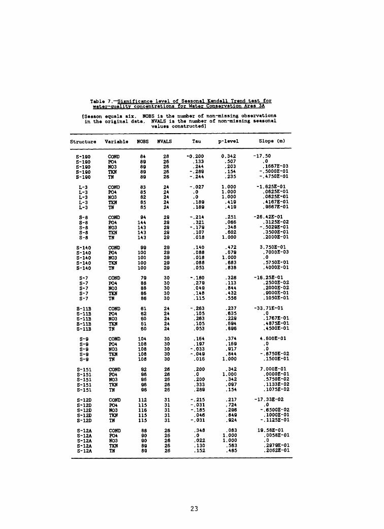
Table 7.—Significance level of Seasonal Kendall Trend test for water-quality concentrations for Water Conservation Area 3A

[Season equals six. NOBS is the number of non-missing observations in the original data. NVALS is the number of non-missing seasonal

values constructed]

Structure

S-190S-190S-190S-190S-190

L-3L-3L-3L-3L-3

S-8S-8S-8S-8S-8

S-1AOS-1AOS-1AOS-1AOS-1AO

S-7S-7S-7S-7S-7

S-11BS-11BS-11BS-11BS-11B

S-9S-9S-9S-9S-9

S-151S-151S-151S-151S-151

S-12DS-12DS-12DS-12DS-12D

S-12AS-12AS-12AS-12AS-12A

Variable

CONDPOAN03TKNTH

CONDPOAN03TKNTN

CONDPOAN03TKNTN

CONDPOAN03TKNTN

CONDPOAN03TKNTN

CONDPOAN03TKNTN

CONDPOAN03TKNTN

CONDPOAN03TKNTN

CONDPOAN03TKNTN

CONDPOAN03TKNTN

NOBS

8A89898989

8385828585

9A1AA1A31A31A3

99100100100100

7988888686

6162606160

10A108108108108

9296969696

112115116115115

8890908989

NVALS

2826262626

2A2A2A2A2A

2929292929

2929292929

3030303030

2A2A2A2A2A

3030303030

2626262626

3131313131

2626262626

Tau

-0.200.133.244

-.289-.2AA

-.027.0.0.189.189

-.21A.321

-.179.107.018

.140

.088

.018

.088

.053

-.180.279.049.148.115

-.263.105.263.105.053

. 16A

.197-.033-.OA9.016

.200

.0

.200

.333

.289

-.215-.031-.185.OA6

-.031

.3A8

.0

.022

.130

.152

p- level

0.3A2.507.203.ISA.235

1.0001.0001.000.419.419

.251

.066

.3A8

.6021.000

.A72

.6791.000.683.838

.326

.113

.844

.A32

.556

.237

.635

.229

.69A

.896

.37A

.169

.917

.8AA1.000

.3421.000.3A2.097.ISA

.217

.72A

.296

.849

.92A

.0831.0001.000.563.A85

Slope (m)

-17.50.0.1667E-03

-.5000E-01-.A750E-01

-1.625E-01.0625E-01.0625E-01.A167E-01.9667E-01

-26.A2E-01.3125E-02

-.5029E-01.3500E-01.2000E-01

3.750E-01.7000E-03.0.5750E-01.AOOOE-01

-16.25E-01.2500E-02.2000E-02.9000E-01.1050E-01

-33.71E-01.0.1767E-01.A875E-01.A500E-01

A.600E-01.0.0

-.8750E-02.1500E-01

7.000E-01.OOOOE-01.5750E-02.1133E-02.1075E-02

-17.33E-02.0

-.6500E-02.1000E-01

-.1125E-01

19.58E-01.0058E-01.0.2979E-01.2062E-01

23

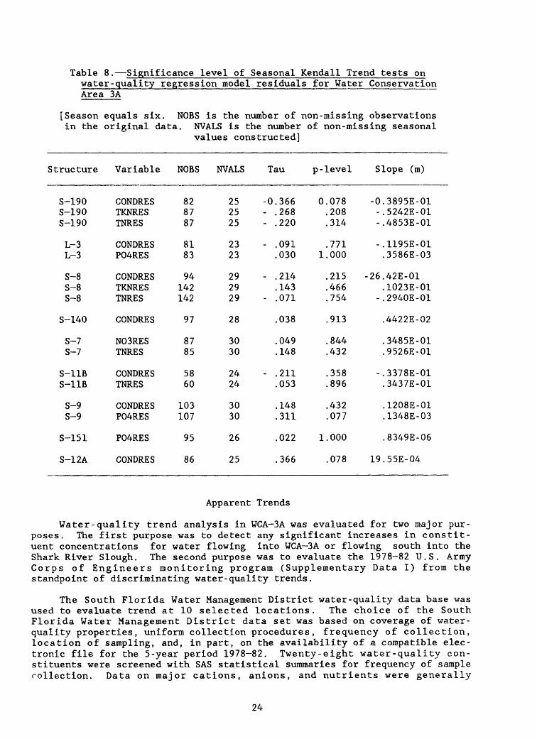
Table 8.—Significance level of Seasonal Kendall Trend tests on water-quality regression model residuals for Water Conservation Area 3A

[Season equals six. NOBS is the number of non-missing observations in the original data. NVALS is the number of non-missing seasonal

values constructed]

Structure Variable NOBS NVALS Tau p-level Slope (m)

S-190 CONDRES 82 25 -0.366 0.078 -0.3895E-01S-190 TKNRES 87 25 - .268 .208 -.5242E-01S-190 TNRES 87 25 - .220 .314 -.4853E-01

L-3 CONDRES 81 23 - .091 .771 -.1195E-01L-3 P04RES 83 23 .030 1.000 .3586E-03

S-8 CONDRES 94 29 - .214 .215 -26.42E-01S-8 TKNRES 142 29 .143 .466 .1023E-01S-8 TNRES 142 29 - .071 .754 -.2940E-01

S-140 CONDRES 97 28 .038 .913 .4422E-02

S-7 S-7

S-11B S-11B

S-9 S-9

S-151

S-12A

N03RES TNRES

CONDRES TNRES

CONDRES P04RES

P04RES

CONDRES

87 85

58 60

103 107

95

86

30 30

24 24

30 30

26

25

.049

.148

- .211 .053

.148

.311

.022

.366

.844

.432

.358

.896

.432

.077

1.000

.078

.3485E-01

.9526E-01

-.3378E-01 .3437E-01

.1208E-01

.1348E-03

.8349E-06

19.55E-04

Apparent Trends

Water-quality trend analysis in WCA—3A was evaluated for two major pur­ poses. The first purpose was to detect any significant increases in constit­ uent concentrations for water flowing into WCA-3A or flowing south into the Shark River Slough. The second purpose was to evaluate the 1978-82 U.S. Army Corps of Engineers monitoring program (Supplementary Data I) from the standpoint of discriminating water-quality trends.

The South Florida Water Management District water-quality data base was used to evaluate trend at 10 selected locations. The choice of the South Florida Water Management District data set was based on coverage of water- quality properties, uniform collection procedures, frequency of collection, location of sampling, and, in part, on the availability of a compatible elec­ tronic file for the 5-year period 1978-82. Twenty-eight water-quality con­ stituents were screened with SAS statistical summaries for frequency of sample collection. Data on major cations, anions, and nutrients were generally

24

available on a frequency of twice per month. Five representative constituents were selected to reduce the amount of data processing and resulting informa­ tion. Models based on 7-, 14-, and 30-day cumulative antecedent rainfall were constructed and the statistically significant models based on r-squared and residual patterns were tested for trend. Orthophosphate and nitrate residuals for 7-day antecedent rainfall at station S—11B were the only two apparent constituent structure pairs that had statistically significant increases.

Plots of the observed concentrations of nitrate and orthophosphate for the 1978-82 collection period at S-6, S-7, and S-11B are shown in figure 11. Unusually high nitrate concentrations were plotted in August 1981. The ex­ tremely high rainfalls that occurred prior to these sample dates reflect Tropical Storm Dennis. The rises in nitrate and orthophosphate concentration during July 1981 shown in figure 11 resulted from the conscious management decision to dewater WCA—2A in 1980 and the controlled burning of much of the area in 1980-81 by the Florida Game and Fresh Water Fish Commission (Worth, 1983). A dry, recently burned area was inundated as a result of more than 11 inches of rainfall on August 16—18, 1981. In addition, the Eastern Everglades Agricultural Area was drained to provide flood relief by pumping water through S-6 and S-7 into WCA-1 and WCA-2A. The high nutrient concentrations of these source waters for S—11B are shown in figure 11. The effects on concentrations were greatly diminished by the next sampling, September 15, 1981. The combi­ nation of a fresh source (the burned marsh area), an extraordinary rainfall (Tropical Storm Dennis) , and enriched agricultural inflow produced highly significant (r 2 - 0.957 for orthophosphate and r 2 - 0.740 for nitrate) quad­ ratic regression models (RSQ7) whose residuals had a significant (p < 0.05) upward trend for the 5-year period 1978-82. The Seasonal Kendall test had been set to season - 6, which means that equivalent 2-month period, median concentration residuals were tested for trend.

The U.S. Army Corps of Engineers sampled for water quality at three locations four times annually (Memorandum of Agreement, Supplementary Data I). The U.S. Army Corps of Engineers, South Florida Water Management District, and National Park Service agreement specified that samples be collected in Octo­ ber, January, April, and July during the period 1978-82. The three locations were all adjacent to Everglades National Park boundaries. The South Florida Water Management District S—11B data were edited to determine whether less frequent sampling would also detect an apparent trend. Samples collected at times approximating the months agreed upon were retained and trend analysis for concentrations and model residuals performed. The trend test was repeated at both season - 6 and season — 4. The results presented in table 9 show no detection of trend with quarterly samples. Changing season from 6 to 4 did not change the lack of significance of either concentration or model residual trends at S-11B.

MONITORING CONSIDERATIONS

The trend analysis approach is almost ideally suited to the South Florida Water Management District computer-based water-quality data management system. The frequency of collection used by South Florida Water Management District is often twice monthly for many important water-quality constituents. This frequent data collection facilitates testing relations with other variables, such as the antecedent rainfall used in this analysis. The South Florida Water Management District water-quality file contains chemical analyses from many locations throughout the district. This widely distributed areal cover­ age provides a distinct advantage in any attempt to analyze water quality superimposed on a complex, highly managed flow system.

25

1978 1979 1980 1981

YEARS

1982

0.80

0.64

0.48

0.32

0.30

0.24

0.18

0.12

0.06

00

A_ J

_l U.UU

LLJ 0.40Q_CO 0.30

< 0.20

<2 0.10

— ' o

I I 1 I 1

-

-

I , I,

S-7

|M i 1

_I

-

IT -

, 1 "

S-11B

1978 1979 1980 1981

YEARS

1982

Figure 11.—Comparison of nitrate and orthophosphate at inflow structure S—11B with two major upstream inflow structures, S6 and S7.

Table 9.—Seasonal Kendall test and slope estimator for trend magnitude at structure S-11B from 1978 through 1982

[NOBS is the number of non-missing observations in the original data. NVALS is the number of non-missing seasonal values constructed]

Variable Season NOBS NVALS Tau p-Level Slope

P04 P04RES

N03 N03RES

2121

1919

1616

1414

0.080.080

.111

.222

0.854.869

.840

.546

0.1000E-29 .1593E-05

.5271E-02

.1301E-01

P04 P04RES

N03 N03RES

2121

1919

1919

1717

.091

.0

.294

.059

.8341.000

.3901.000

1000E-29 2587E-04

5000E-02 6459E-02

26

Several aspects of the South Florida Water Management District water- quality monitoring network correspond to components of an idealized network similar to that shown in figure 12. Wide geographic distribution enhances identification of a chemical constituent close to the source of the constit­ uent. The combination of extensive coverage of water-quality constituents, frequent sample collection, and rapid chemical analyses increases the lead time for affecting contaminant containment or dispersal. A frequent sample collection program also permits a water-quality data base that provides a more robust statistical analysis of changes (trend analysis) and the factors such as antecedent rainfall or discharge that might influence change.

ECOLOGICAL PERSPECTIVE

EXTENSIVE PARAMETER COVERAGE

WIDER FREQUENTGEOGRAPHIC SAMPLEDISTRIBUTION COLLECTION

WETLAND \ RESEARCH/

RESOURCE CONSTRAINTS

CONTINUINGDATA

ANALYSIS

/CONTAMINANTS VMANAGEMENT/

RAPID CHEMICAL ANALYSIS

EXPLANATION

-^- MAJOR PATHWAY

->- ALTERNATIVE PATHWAY

DATA MANAGEMENT SYSTEM

Figure 12.—Schematic representation of the components of an idealized water-quality monitoring network.

The U.S. Army Corps of Engineers data-collection effort included analyses for 36 water-quality constituents and 21 individual pesticides. Extensive coverage on a watershed like the Shark River Slough provides resource managers with information on changes from a wide variety of sources in the basin. The cost of extensive coverage on a frequent sample-collection interval is exces­ sive and diverts laboratory facilities and personnel resources from other responsibilities. The idealized water-quality monitoring network would use water-quality surrogates for extensive coverage. This approach was agreed to in the 1979 Memorandum of Agreement by specifying daily samplings for dis­ solved oxygen, specific conductance, and pH. The twice monthly collection of nutrients and other constituents by South Florida Water Management District accomplishes a similar goal. The revised Memorandum of Agreement of 1984 incorporated the concepts of more frequent sample collection, more sample collection locations, and fewer types of chemical analyses.

27

Many of the objectives of an idealized water-quality monitoring network depend on two attributes that are facilitated by current laboratory technol­ ogy; rapid chemical analyses and storage of the results in an accessible computerized data-management system. The U.S. Army Corps of Engineers results could not be readily analyzed because four different types of data storage and retrieval were used in the 5-year period covered by the 1979 Memorandum of Agreement. Rapid access to the analytical results of any monitoring system facilitates recall of previous results and testing for change. Continuing data analysis not only recognizes change but permits revisions to the judi­ cious use of surrogates and allows sample collection adjustments to more clearly characterize water-quality changes.

Ecological perspective is a component of the idealized water-quality monitoring network to the extent that the network sampling strategy may be revised. Judgments of sampling location, frequency, parameter coverage, type of data analysis, and use of surrogates, all depend on understanding how the entire ecological system functions. This understanding needs to be revised by a continuing data analysis of the network. ^ series of research programs, external to the monitoring network, designed to determine the biogeochemical processes that operate in southern Florida would enhance a reevaluation of sampling strategy.

CONCLUSIONS

The specific approach of model construction and Seasonal Kendall trend analysis is but one type of continuing data analysis. The trend analysis approach is applied to a single constituent and station versus time and cannot address the marked concentration gradient that exists across the water conser­ vation flow system. The trend analysis of samples from 10 flow structure locations around WCA—3A leads to a number of conclusions:

• It is possible to amend the Seasonal Kendall trend procedure used by the U.S. Geological Survey to a more generalized approach for data sets with other data formats.

• The application of model construction and Seasonal Kendall test for trend to the South Florida Water Management District data bases was successful.

• Antecedent rainfall and water-quality constituent regression models were constructed for 10 flow stations. Only 17 statistically significant regression models from 350 possible combinations were available for trend analysis.

• No trends for specific conductance, orthophosphate-phosphorus, nitrate- nitrogen, total Kjeldahl nitrogen, or total nitrogen were detected by the Seasonal Kendall test for the 1978—82 time period at the 10 flow struc­ tures .

• An apparent trend for orthophosphate-phosphorus and nitrate-nitrogen ini­ tially seen at S—11B was not accepted because of the influence of out­ liers. Elimination of outliers eliminated the statistical significance of the apparent trend.

• Monthly or more frequent sample collection is highly desirable for trend analysis.

28

• Although pronounced areal differences in water quality exist around Water Conservation Area 3A, no water-quality trends were detected adjacent to the agricultural areas for the 1978-82 time period.

• Discharge was excluded from the evaluation of models because specific changes were made in the release strategy during the evaluation period. If water release followed a consistent set of rules during an evaluation period, then discharge could be a basis for trend evaluation.

The S-12 outflow structures yielded the fewest statistically significant regression models, possibly because the flow regulation was independent of rainfall and the Conservation Area which contributes flow is a large flood pool that is independent of short term (30 days or less) rainfall.

On the basis of this analysis, certain aspects of an ideal water-quality monitoring network for the Shark River Slough can be defined. These include:

• A computerized data-management system is needed for this and many other rigorous evaluation programs.

• Each station has distinguishable water-quality characteristics that suggest that the number of sample locations is important and that lumping of inflow data needs to be done cautiously in any evaluation effort.

• Location of sampling sites away from Shark River Slough and closer to source areas of nutrients and other chemical constituents affords early identification of problems and possible ameliorative response.

• Coordination between the Everglades National Park, South Florida Water Management District, and U.S. Army Corps of Engineers is highly desirable for any water-quality monitoring network for Shark River Slough.

REFERENCES

Bowker, A.H., and Liberman, G.J., 1972, Engineering statistics, (2d ed.):Englewood, N.J., Prentice-Hall, Inc., p. 475-481.

Crawford, C.G. , Slack, J.R., and Hirsch, R.M. , 1983, Nonparametric tests fortrends in water-quality data using the statistical analysis system: U.S.Geological Survey Open-File Report 83-550, 102 p.

Daniel, Cuthbert, and Wood, F.S., 1971, Fitting equations to data: New York,Wiley-Interscience, 342 p.

Federico, A.C., Millar, P.S., and Davis, F.E., in press, Water quality andnutrient loading analysis of the Water Conservation Areas, 1978-1983:South Florida Water Management District Technical Publication 87-X.

Flora, M.D., and Rosendahl, P.C. , 1981, The response of specific conductanceto environmental conditions in the Everglades National Park, Florida:Water, Air, and Soil Pollution, v. 16, p. 159-175.

Helwig, J.T., and Council, K.A. , eds., 1979, The SAS user's guide, 1979 edi­ tion: Gary, N.C., SAS Institute, Inc., 494 p.

Hirsch, R.M., Slack, J.R., and Smith, R.A., 1982, Techniques of trend analysisfor monthly water-quality data: Water Resources Research, v. 18, no. 1,p. 107-121.

Kendall, M.G. , 1975, Rank correlation methods: London, Charles Griffin andCo., Ltd., 202 p.

29

Lin, Steve, Lane, Jim, and Marban, Jorge, 1984, Meteorological and hydrologi- cal analysis of the 1980-1982 drought: South Florida Water Management District Technical Publication 84-7, 42 p.

Rosendahl, P.C., and Rose, P.W. , 1979, Water quality standards: Everglades National Park: Environmental Management, v. 3, no. 6, p. 483-491.

Swift, D.R., 1981, Preliminary investigations of periphyton and water quality relationships in the Everglades Water Conservation Areas: South Florida Water Management District Technical Publication 81-5, 124 p.

Waller, B.C., and Earle, J.E., 1975, Chemical and biological quality of water in part of The Everglades, southeastern Florida: U.S. Geological Survey Water-Resources Investigations 56-75, 157 p.

Worth, Dewey, 1983, Preliminary environmental responses to marsh dewatering and reduction in water regulation schedule in Water Conservation Area 2A: South Florida Water Management District Technical Publication 83-6, 63 p.

30

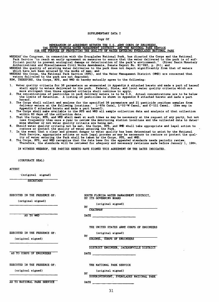
SUPPLEMENTARY DATA I

Copy Of

MEMORANDUM OF AGREEMENT BETWEEN THE U.S. ARMY CORPS OF ENGINEERS. THE SOUTH FLORIDA WATER MANAGEMENT DISTRICT. AND THE NATIONAL PARK SERVICE

FOR THE PURPOSE OF PROTECTING THE QUALITY OF WATER ENTERING EVERGLADES NATIONAL PARK

WHEREAS*the Congress, in connection with the Everglades National Park, has directed the Corps and the National Park Service "to reach an early agreement on measures to assure that the water delivered to the park is of suf­ ficient purity to prevent ecological damage or deterioration of the park's environment." (River Basin Monetary Authorizations and Miscellaneous Civil Works Amendments, Senate Report No. 91—895, p. 24); and

WHEREAS the quality of existing water deliveries to the park does not depart significantly from that of waters which have not been altered by the works of man; and

WHEREAS the Corps, the National Park Service (NFS), and the Water Management District (WMD) are concerned that waters delivered to the park are not degraded;

NOW, THEREFORE, the Corps, NPS, and WMD do hereby mutually agree to the following:

1. Water quality criteria for 36 parameters as enumerated in Appendix A attached hereto and made a part of hereof shall apply to waters delivered to the park. Federal, State, and local water quality criteria which are more stringent than those appended criteria shall continue to apply.

2. The concentrations of pesticides in park delivery waters is to be 0.0. Actual concentrations are to be below the limits of detection. A listing of pesticides is shown in Appendix B attached hereto and made a part hereof.

3. The Corps shall collect and analyze for the specified 36 parameters and 21 pesticide residues samples from delivery waters at the following locations: L~67A Canal, L~31~W Canal, and C~111 Canal. (See map in Appendix C attached hereto and made a part hereof).

4. The Corps shall make available to the NPS and WMD all sample collection data and analysis of that collection within 60 days of the collection date.

5. That the Corps, NPS, and WMD shall meet at such times as may be necessary at the request of any party, but not less frequently than once a year to review the monitoring station locations and the collected data to deter­ mine whether or not water quality criteria are being met.

6. Should water quality criteria not be met, the Corps, NPS, and WMD shall take appropriate and legal action to restore or protect the quality of water entering the Park.

7. In the event that a clear and present danger to water quality has been determined to exist by the NationalPark Service, appropriate actions or such legal process as may be necessary to restore or protect the qual­ ity of water entering the Park shall be taken by the Corps, NPS, and WMD.

8. The Corps, NPS, and WMD recognize that the data base for the appended standards needs periodic review.Therefore, the standards will be reviewed for adequacy and necessary revisions made before January 1, 1984.

IN WITNESS WHEREOF, THE PARTIES HERETO HAVE SIGNED THIS AGREEMENT ON THE DATES INDICATED.

(CORPORATE SEAL)

ATTEST

{original signed)

SECRETARY

EXECUTED IN THE PRESENCE OF:

(original signed)

AS TO WMD

SOUTH FLORIDA WATER MANAGEMENT DISTRICT, BY ITS GOVERNING BOARD

BY(original signed)

CHAIRMAN

DATE

EXECUTED IN THE PRESENCE OF:

(original signed)

AS TO CORPS OF ENGINEERS

THE UNITED STATES ARMY CORPS OF ENGINEERS

(original signed)BY _______________________________

COLONEL, CORPS OF ENGINEERS

DISTRICT ENGINEER, JACKSONVILLE DISTRICT

DATE

EXECUTED IN THE PRESENCE OF:

(original signed)

AS TO NATIONAL PARK SERVICE

BY

THE NATIONAL PARK SERVICE

(original signed)

SUPERINTENDENT, EVERGLADES NATIONAL PARK

DATE

31

SUPPLEMENTARY DATA I.——Copy Of: OF ENGINEERS. THE SOUTH FLORIDA

BETWEEN THE U.S. ARMY CORPSAND THE NATIONAL

SERVICE THE PURPOSE OFNATIONAL PARK—Continued

WATER ENTERING EVERGLADES

APPENDIX A

Parameter

Turbidity, JTUColor, PCUSpec. Conductance (umho)DO, mg/LBOD, mg/LNH4, mg/L, as NN02, mg/L, as NN03, mg/L, as NOrgN, mg/L, as NTotal N, mg/L, as NP04, mg/L, as PTotal P, mg/L, as PTOC, mg/LTIC, mg/LpH, UnitsAlkalinity, mg/L, as CaC03TDS, mg/LHardness, mg/L, as CaC03Non carb Hard, mg/LCalcium, mg/LMagnesium, mg/LSodium, mg/LPotassium, mg/LChloride, mg/LSulfate, mg/LFluoride, mg/LArsenic, Mg/LCadmium, pg/LChromium, pg/LCobalt, MS/LCopper, pg/LIron, pg/LLead, pg/LManganese, pg/LZinc, jig/LMercury, pg/L

Mean concentration 1970-1978

X

4.4465.56573.65.181.42.089.0128.16

1.521.8.008.033

32.740.47.8

176.9344.81741958.311.3472.977.619.7

.357.82.23.51.22.4

1224.210.519.6

.07

Upper limit 1L

11124647

4.530.240.040.72.1

I 2.90.020.24

51607.6-8.0269566330548625935

143540.7

20102058

2701324720.5

Annual mean not to exceed this value. All parameters measured quarterly (October, January, April, and July) except Dissolved Oxygen, Specific Conductance, and pH, which are to be measured daily.

APPENDIX B

Pesticides Allowable Concentration of Zero 1 (Sampled Semiannually)

Parameter

AldrinLindane

ChlordaneDDDDDEDDT

DieldrinEndrinEthion

ToxapheneHeptachlor

Heptachlor EPCB

MalathionParathionDiazinon

Methyl Parathion2, 4, 5 - T

SilvexTrithion

Methyl Trithion

Samples to be taken in water column until concentrations in sediment are established.

32

SUPPLEMENTARY DATA II.--Card image formats of South Florida Water Management District water-quality data set (WCAQW)and discharge data set.

Station number iDatel

1 1

CAMB0163L3 1.0478 .

I Orthophosphate 1 Phosphorus 1

1445 .000CAMB0163L3CAMB0163L3 .004 [CAMB0163L3CAMB0163L3CAMB0163L3CAMB0259L3 11878.

.024t

(Nitrate19

1600.000.000

CAMB0259L3CAMB0259L3 .004 .004

0.000.067

J .040

17 200109010

[Conductance 1

6.7001

i

470.00

|1.200|

0

142.

7.300

.190 1.230100

TotalKjeldahlNitrogen

*• [Sample Type CodeoTooo.016.020

18 800041010

9.100

1.010

490.000

CAMB0259L31

42

7.7004

.000 1.020

.800

>- NextSample

CAMB0259L3CAMB0259L3 19

Daily discharge (cubic feet

L378011L378012

34

L378013 192L378021L378022L378023L378031L378032L378033

000000

.000

per

15

194000000

second) in three card per

06

010

143 133000000

000000

08

118000000

08

114000000

month

05

134000000

format with implicit date.

06

132000000

1 46 69

95 900 00 0

0 00 00 0

95

0

Data File Name: WCAQW

Content: Water quality data at S-7, S-8, S-9, S-11B, S-12A, S-12D, S-140, L-3, L-28, S-151 for period 1978 through 1982.

Input Format:

(Comment)

(hours, min)(meters)(°C)

(fieldmeasure­ment)

(totaldissolvedP)

(dissolvedorganic P)

(particulateP)

(totalorganiccarbon)

VariableName

STATIONMONTHDAYYEARTIMEDEPTHTEMPDO

SECONDLABCONDPHTURBCOLOROP04TP04

TDP04

DORGP04

PARTP

TOTORGCN02N03

RecordNo,

11111111

1112222

2

2

2

233

ColumnsBegin

918202225334149

57657317253341

49

57

65

731725

End

1219212328404856

64728024324048

56

64

72

802432

FieldWidth

41224888

8888888

8

8

8

888

Type

AFFFFFFF

FFFFFFF

F

F

F

FFF

(Comment)

(NOx + NH4)

(dissolvedTKN)

(TKN-NH4)

(hardness)

VariableName

INORGNH4TKN

TDKNORGNTOTALNCAMGKNASI02S04CLALKHARD

RecordNo.

333

333444444445

ColumnsBegin

334149

576573172533414957657217

End

404856

647280243240485664728024

FieldWidth

888

888888888888

Type

FFF

FFFFFFFFFFFF

(total dissolved:cadmiumchromiumcoppermanganeseleadstrontiumzinc)

1 -discharge,2-nodischarge

sample type

TDISSCDTDISSCRTDISSCUTDISSMNTDISSPBTDISSSRTDISSZN

DSCHSAMTYP

5555555

66

25334149576573

1725

32404856647280

2432

8888888

88

FFFFFFF

FF

Equivalent Fortran Format: (8X,A4,3F2,F4.0,4X,6F8.3/16X,8F8.3/16X,8F8.3/16X, 8F8.3/16X.8F8.3/16X.3F8.3

Note on Sample Type (SAMTYP): delete all observations with SAMTYP • 9. These represent duplicate analyses. All other values represent valued data.

Number of card images: 22.242

33

SUPPLEMENTARY DATA III.—Listing of TRANSPOSE program written by Sharon Watkins, U.S. Geological Survey.

//AG41CAR5 JOB (account number,MATTR,3,10).'MATTRAW.// CLASS-T//* $$DIR <TPA>TALLAHASSEE>STUDIES>HMATTRAW>SFWMD// EXEC SAS//DISCH DD DSN-AG41CAR.QL3.DATA,DISPHDLD,UNIT-ONLINE//OUTR DD DSN-AG41CAR.FLOW,DISP-OLD,// UNIT-ONLINE//SYSIN DD *DATA Q;INFILE DISCH*

INPUT YEAR1 10-11 M01 12-13 615 (V1-V10) (10*6.)#2 615 (V11-V20) (10*6.)#3 615 (V21-V31) (10*6.);

PROC TRANSPOSE PREFIX-Q OUT-QPRIME; VAR V1-V31;BY YEAR1 M01;

PROC MATRIX; DUMMY-J(1860,1); DO 1-1 TO 5; Dp J-l TO 12; DO K-l TO 31;DUMMY((((((I-

END; END;

END;OUTPUT DUMMY OUT-DATES (RENAME-(COL1-DATE)); DATA OUTR.QL3;MERGE QPRIME DATES; IF Ql- . THEN DELETE; DROP NAME_ ROW;

PROC PRINT ; /*

SUPPLEMENTARY DATA IV.—Listing of MERGE program written by Sharon Watkins,U.S. Geological Survey.

//AG41CAR5 JOB (account number.MATTR,5,10),'MATTRAW', // CLASS-S//*$$DIR <TPA>TALLAHASSEE>STUDIES>HMATTRAW // EXEC SAS//DISCH DD DSN-AG41CAR.FLOW,DISP-OLD //GLADES DD DSN-AG41CAR.S7.DATA,DISP-OLD //RAIN DD DSN-AG41CAR.FLOW,DISP-OLD //MRG DD DSN-AG41CAR.FLOW,DISPHDLD //SYSIN DD * DATA ONE;SET RAIN.RF99;RF7T-LAG(RF1 )+LAG2(RF1HLAG3(RFD+LAG4 (RF1 )+LAG5(RF1 )HJM56(RF1 )+LAG7 (RF1); RF14T-RF7T+LAG8(RF1)+LAG9(RF1)-I-LAG10(RF1)+LAG11(RF1)+LAG12(RF1)+ LAG13(RF1)-I-LAG14(RF1);RF30T-RF14T+LAG15(RF1)+LAG16(RF1)+LAG17(RFD+LAG18(RF1)+LAG19(RF1)+ LAG20(RFl)-l-LAG21(RFl)-l-LAG22(RFl)+LAG23(RFl)-l-LAG24(RFl)+LAG25(RFl)+LAG26(RFl)+ LAG27 (RF1 )+LAG28 (RF1 )+LAG29 (RF1 )-l-LAG30 (RF1); DATA TWO;SET DISCH.QS7;Q7T-LAG(Q1)+LAG2(Ql)+LAG3(Ql)+LAG4(Ql)+LAG5(Ql)+LAG6(Ql)+LAG7(Ql); IF Q7T-0 THEN DO; Q7T-2;

END;Q14T-Q7T+LAG8(Q1)-I-LAG9(Q1)+LAG10(Q1)-I-LAG11(Q1)+LAG12(Q1)+ LAG13(Q1)-I-LAG14(Q1);Q30T-Q14T+LAG15(Ql)+LAG16(Ql)+LAG17(QlHLAG18(Ql)+LAG19(Ql)+ LAG20(Ql)+LAG21(Ql)+LAG22(Ql)+LAG23(Ql)+LAG24(Ql)+LAG25(Ql)+LAG26(Ql)+ LAG27(Q1)+LAG28(Q1)-I-LAG29(Q1)+LAG30(Q1); i DATA THREE;INFILE GLADES; INPUT ID $ 9-12 M01 18-19 DATE 20-21 YEAR1 22-23 COND 57-64#2 P04 33-40#3 N03 25-32 TKN 49-56 TN 73-80#6;PROC SORT; BY YEAR1 M01 DATE;DATA MRG.MS7; MERGE ONE TWO THREE; BY YEARl M01 DATE!IF (COND-. & P04-. & N03-. & TKN-. & TN-.) THEN DELETE;OUTPUT MRG.MS7;/*

34

SUPPLEMENTARY DATA V.—Listing of MAXR program with rainfall only independentvariable

//AG41CAR5 JOB (account number,MATTR,3,10),'MATTRAW', // CLASS-C//* $$DIR <TLH>TALLAHASSEE>STUDIES>HMATTRAW>STEP // EXEC SAS//MRG DD DSN-AG41CAR.FLOW,DISP-OLD,UNIT-ONLINE //SYSIN DD * DATA ONE; SET MRG.ML3;

IF RF7T-0.00 THEN DO;RF7T-0.01;

END;IF RF14T-0.00 THEN DO;RF14T-0.02;

END;IF RF30T-0.00 THEN DO;RF30T-0.03;

END;IF P04-0.002 THEN DO;

P04-0.004; END;

LNRF7-LOG(RF7T); LNRF14-LOG(RF14T); LNRF30-LOG(RF30T); INVRF7-1/RF7T; INVRF14-1/RF14T; INVRF30-1/RF30T; LNCOND-LOG(COND); LNP04-LOG(P04); LNN03-LOG(N03); LNTKN-LOG(TKN); LNTN-LOG(TN); DATR=MDY(M01,DATE,YEAR1); JULIAN-JULDATE(DATR); DOY^MOD(JULIAN,1000);IF MOD(YEAR1,4)-0 THEN DECTIME-1900+YEARl+(DOY/366); ELSE DECTIME-1900+YEARl+(DOY/365); PROC SORT;BY JULIAN; PROC STEPWISE; MODEL LNCOND-LNRF7 LNRF14 LNRF30 RF7T RF14T RF30T INVRF7 INVRF14 INVRF30/

MAXR STOP-1; DATA TWO; SET ONE; PROC STEPWISE; MODEL LNP04-LNRF7 LNRF14 LNRF30 RF7T RF14T RF30T INVRF7 INVRF14 INVRF30/MAXR STOP-1;

DATA THREE;SET TWO; PROC STEPWISE; MODEL LNN03-LNRF7 LNRF14 LNRF30 RF7T RF14T RF30T INVRF7 INVRF14 INVRF30/MAXR STOP-1;

DATA FOUR;SET THREE; PROC STEPWISE; MODEL LNTKN-LNRF7 LNRF14 LNRF30 RF7T RF14T RF30T INVRF7 INVRF14 INVRF30/MAXR STOP-1;

DATA FIVE;SET FOUR; PROC STEPWISE; MODEL LNTN-LNRF7 LNRF14 LNRF30 RF7T RF14T RF30T INVRF7 INVRF14 INVRF30/MAXR STOP-1;

/*

35

SUPPLEMENTARY DATA VI.—Listing of GLM program with Seasonal Kendall test attached

//AG41CAR5 JOB (account number,MATTR,3,10),'MATTRAW', // CLASS-C//* $$DIR <TLH>TALLAHASSEE>STUDIES>HMATTRAW>GLM //PROCLIB DD DSN-WRD.FRQCLIB,DISP-SHR // EXEC WRDSAS,DSN1-NULLFILE,DSN2-NULLFILB //MRG DD DSN-AG4ICAR.FLOW,DISP-OLD,UNIT-ONLINE //SYSIN DD * OPTIONS NOOVP NODATE; DATA ONE; SET MRG.MS11B;

IF RF7T-0.00 THEN DO;RF7T-0.01;

END;IF RFUT-0.00 THEN DO;RF14T-0.02;

END;IF RF30T-0.00 THEN DO;RF30T-0.03;

END;IF P04-0.002 THEN DO;

P04-0.004; END;

LNCOND-LOG(COND); RSQ7-RF7T*RF7T; DATR-WDY(M01,DATE,YEAR1); JULIAN-JULDATE(DATR); DOY-MODC JULIAN, 1000);IF MOD(YEAR 1,<O-0 THEN DECTIME-1900+YEARl+(DOY/366); ELSE DECTIME-1900+YEAR1+CDOY/365); PROC SORT;BY JULIAN; PROC GLM;MODEL LNCOND-RF7T; OUTPUT OUT-B

PREDICTED-CONDPRED RESIDUAL-CONDRES; PROC SEASKEN SEASON-6; VAR DECTIME COND CONDRES;

PROC PLOT NOLEGEND; PLOT CONDRES*DECTIME CONDRES*CONDPRED;

TITLE1 GLM RESIDUALS VERSUS DECTIME FOR SUB; PLOT LNCOND*DECTIME-'0' CONDFRED*DECTIME-'P' / OVERLAY;

TITLE1 OBSERVED AND PREDICTED CONDUCTANCE VERSUS DECTIME FOR SUB; DATA TWO; SET ONE; PROC GLM; MODEL P04-RSQ7; OUTPUT OUT-B

PREDICTED-POWERED RESIDUAL-P04RES; PROC SEASKEN SEASON-6; VAR DECTIME P04 P04RES;

PROC PLOT NOLEGEND; PLOT P04RES*DECTIME P04RES*P04PRED;

TITLE1 GLM RESIDUALS VERSUS DECTIME FOR SUB; PLOT P04*DECTIME-'0' P04PRED*DECTIME-'P I / OVERLAY;

TITLE1 OBSERVED AND PREDICTED ORTHOPHOSPHATE VERSUS DECTIME FOR SUB; DATA THREE;SET TWO; PROC GLM; MODEL N03-RSQ7;

OUTPUT OUT-BPREDICTED-N03PRED RESIDUAL-N03RES; PROC SEASKEN SEASON-6;

VAR DECTIME N03 N03RES; PROC PLOT NOLEGEND;

PLOT N03RES*DECTIME N03RES*N03PRED; TITLE1 GLM RESIDUALS VERSUS DECTIME FOR SUB;

PLOT N03*DECTIME-'0' N03PRED*DECTIME-'P' / OVERLAY;TITLE1 OBSERVED AND PREDICTED NITRATE VERSUS DECTIME FOR SUB;

DATA FOUR;SET THREE;PROC SEASKEN SEASON-6; VAR DECTIME TKN;

PROC PLOT NOLEGEND; PLOT TKN*DECTIME;

TITLE1 TOTAL KJELDAHL NITROGEN VERSUS DECTIME FOR SUB; DATA FIVE;SET FOUR; PROC GLM;

MODEL TN-RSQ7; OUTPUT OUT-B

PREDICTED-TNPRED RESIDUAL-TNRES; PROC SEASKEN SEASON-6;

VAR DECTIME TN TNRES; PROC PLOT NOLEGEND; PLOT TNRES*DECTIME TNRES*TNPRED;

TITLE1 GLM RESIDUALS VERSUS DECTIME FOR SUB; PLOT TN*DECTIME-'0' TNPRED*DECTIME-'P' / OVERLAY;

TITLE1 OBSERVED AND PREDICTED TOTAL NITROGEN VERSUS DECTIME FOR SUB; PLOT RF7T*DECTIME RSQ7*DECTIME; /* //

36

SUPPLEMENTARY DATA VII.—Residual plots for the 30 statistically significantregression models.

Residual versus predicted:

Conductance for S190Orthophosphate for S190Total Kjeldahl nitrogen for S190Total nitrogen for S190Conductance for L3Orthophosphate for L3Total nitrogen for L3Conductance for S8Orthophosphate for S8Nitrate for S8Total Kjeldahl nitrogen for S8Total nitrogen for S8Conductance for S140Orthophosphate for S140Conductance for S7Orthophosphate for S7Nitrate for S7Total Kjeldahl nitrogen for S7Total nitrogen for S7Conductance for SUBOrthophosphate for SUBNitrate for SUBTotal nitrogen for SUBConductance for S9Orthophosphate for S9Nitrate for S9Orthophosphate for S151Conductance for S12DOrthophosphate for S12DConductance for S12A

37

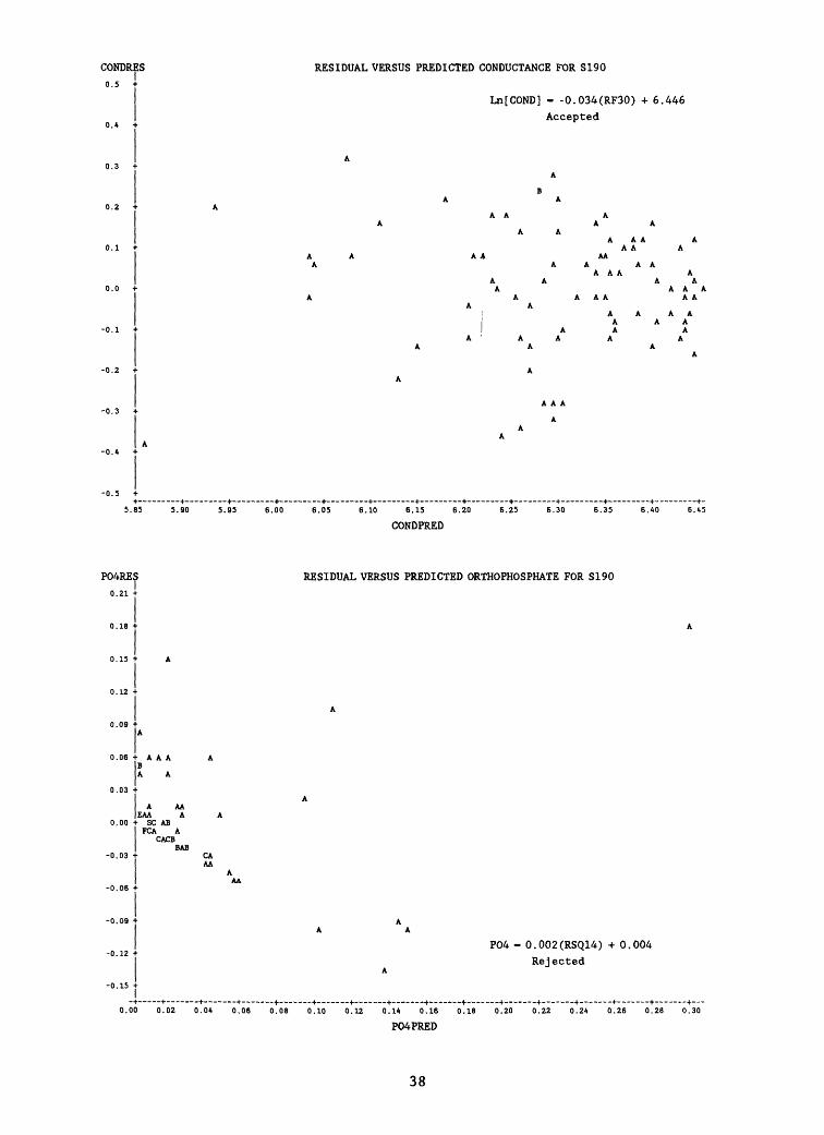
CONDRES

0.5 +

RESIDUAL VERSUS PREDICTED CONDUCTANCE FOR S190

Ln[COND] - -0.034(RF30) + 6.446

Accepted

A A A AA A A

AA A A AA A A A

A AA A A

A A A A

A A A A A A A

A A A

A

5.65 5.90 5.95 6.00 6.05 6.10 6.15

CONDPRED

6.20 6.25 6.30 5.35 6.40

P04RES

0.21

0.00

A A A ABA A

A AAEAA A

• SC AB FCA A

CACBBAB

CA AA

RESIDUAL VERSUS PREDICTED ORTHOPHOSPHATE FOR S190

P04 - 0.002(RSQ14) +0.004 Rejected

0.00 0.02 0.04 0.06 0.08 0.10 0.12 0.14 0.16 0.18 0.20 0.22 0.24 0.26 0.28 0.30

P04PRED

38

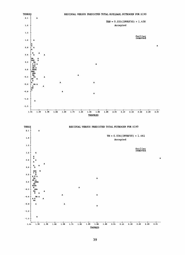
TKNRES 2.1 + A

o.o

BA A BAB A

• BA AAA AAA AB A

• BCBA BAA

AEABA

• CA DB A

A A

• AA AA

AB A

RESIDUAL VERSUS PREDICTED TOTAL KJELDAHL NITROGEN FOR S190

TKN - 0.035(INVRF30) + 1.438

Accepted

Outlier removed

1.44 1.50 1.56 1.62 1.68 1.74 1.80 1.86 1.92 1.98 2.04 2.10 2.16 2.22 2.28 2.34

TKNPRED

TNRES 2.1 + A

1.2 + A

A A

0.9 + A A

A A0.6 + B

0.3

-0.3

AAA B C B

B B B A

BA AB A

0.0 + ABBADA

BCAAB

ABAEA A

B A

-0.6 + BA AA A A AA

RESIDUAL VERSUS PREDICTED TOTAL NITROGEN FOR S190

TN - 0.036(INVRF30) + 1.461

Accepted

Outlier removed

1.44 1.50 1.56 1.62 1.68 1.74 1.80 1.86 1.92 1.98 2.04 2.10 2.16 2.22 2.28 2.34

TNPRED

39

CONDRES

-0.3

-0.7 +

RESIDUAL VERSUS PREDICTED CONDUCTANCE FOR L3A A

A

AAA A

A A A A

A AAA A

AA A

A BAA A

A A A A A A

BA

A A

Ln(COND) - -0.058(RF30) + 6.263

Accepted

5.2 5.3 5.4 5.5 5.6 5.7 5.8

CONDPRED

6.0 6.1 5.2 6.3

P04RES

0.30

-0.05

AA A A

A

A BB

RESIDUAL VERSUS PREDICTED ORTHOPHOSPHATE FOR L3

A

P04 - 0.001(RSQ30) +0.016

Rejected

Ln(P04) - 0.028(RF30) - 4.815

Accepted

BBA AA AAA A A A

0.00 + DBACHCA AA A A A

CBBAA A A C A

A A AAB

-0.20_+—————+———————+..

0.00 0.05 0.10 0.15 0.20 0.25 0.30 0.35 0.40 0.45 0.50 0.55 0.60

P04PRED

40AU.S. GOVERNMENT PRINTING OFFICE: l 9 8 7.5 3 o.l 0 VS 0 o o 8

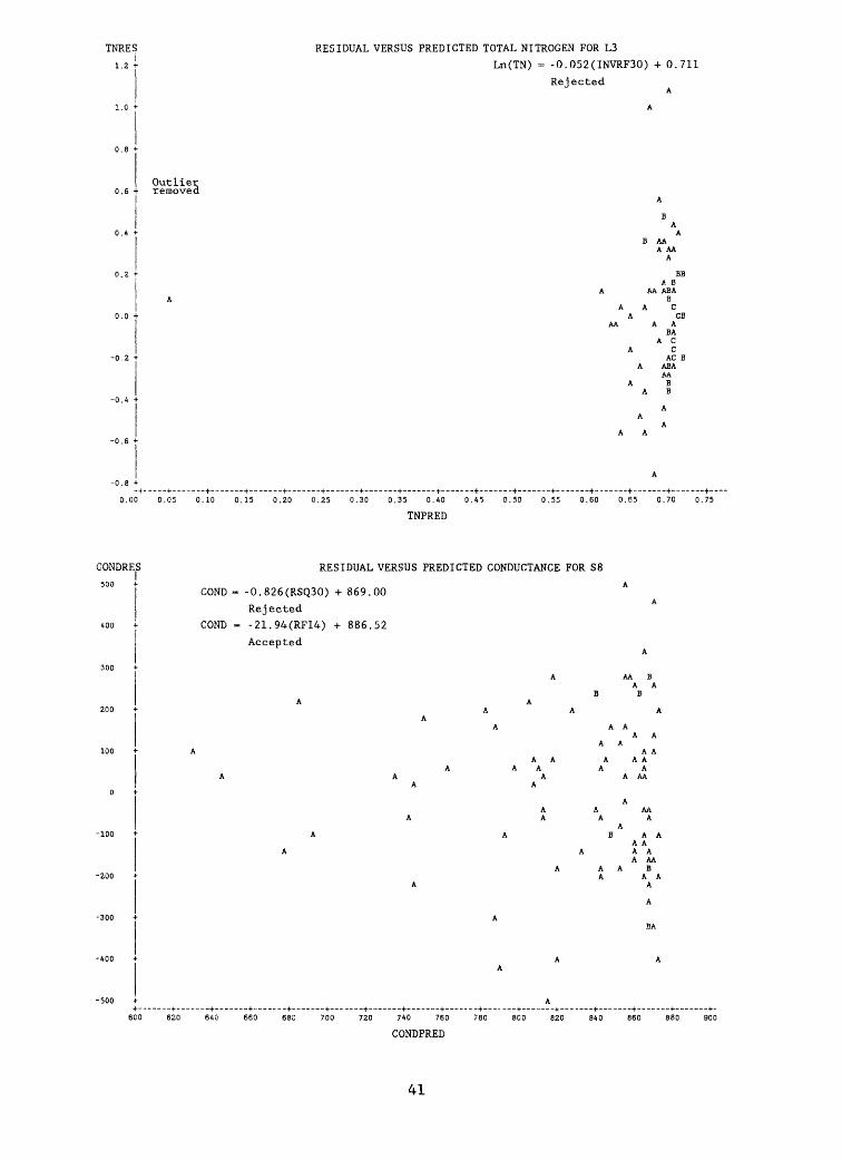
TNRES

1.2

RESIDUAL VERSUS PREDICTED TOTAL NITROGEN FOR L3

Ln(TN) - -0.052(INVRF30) + 0.711

Rejected

Outlier .6 + removed

B AAA AA

A

A B A AA ABA

B A A C

A CBAA A A

BAA C

A CAC B

A ABAAA

A B A B

A A

A

0.00 0.05 0.10 0.15 0.20 0.25 0.30 0.35 0.40 0.45 0.50 0.55 0.60 0.65 0.70 0.75

TNPRED

CONDRES500 +

RESIDUAL VERSUS PREDICTED CONDUCTANCE FOR S8

COND - -0.826(RSQ30) + 869.00

Rejected

COND - -21.94(RF14) + 886.52

Accepted

A A A A

AA

AA B A A

A AA A

A AA A

A A AA A

A AA

A A AA A A A

A B A A

A A A A A

A AA A A A B

A A A A

A

BA

600 620 640 660 680 700 720 740 760 780 800 820 840 860 880 900

CONDPRED

41

P04RES5 •*-

RESIDUAL VERSUS PREDICTED ORTHOPHOSPHATE FOR S8

Ln(P04) - 0.198(RF30) - 5.418

Rejected

* AA * *A A A A

A AA A A AA A A

B A A A AAAAA A AA A A A

A B AA A A A

A A A A AA A A A A A A

A A A A AA AD A

BBBC A A A B A CB BA

A ACC A A A AA A DC A A

AA AAA

A A A

-5 •*-—+————_-+—. — _—+—— — — _+—-6,0 -5.7 -5.* -5.1 -4.5 -it.2 -3.9

P04PRED

-3.G -3.3 -3.0 -2.7 -2.* -2.1

N03RES

4.0

-0.5 ••

AA

AA

BA A BAA A BAA A

BB A BOB A B

EA A D AHCAB AA KCAA A

JCAA A A CB AA

A AA

AA A

RESIDUAL VERSUS PREDICTED NITRATE FOR S8

N03 - 0.065(RSQ7) + 0.565

Rej ected

2.0 Z.It 2.f

N03PRED

42

TKNRES

1.50

1.25

0.00 + A A B C

-0.25

-0.50

RESIDUAL VERSUS PREDICTED TOTAL KJELDAHL NITROGEN FOR S8

Ln(TKN) - 0.061(LNRF14) +0.888 Accepted

A AA A AA B

A A B A A AA A

A B A A A A A AA

A AB A

BAA AAAAA ACAAA

A A A A A A A AAA

AAA A A A

A AAA A A

AAAA

A A A

A A

A A

,68 0.71 0.74 0.77 0.80 0.83 0.88 0.89 0.92 0.95 0.98 1.01 1.04

TKNPRED

TNRES

7 +RESIDUAL VERSUS PREDICTED TOTAL NITROGEN FOR S8

TN - 0.530(RF7) + 2.803

Accepted

A A AAA A

A A A

A

A ABA A

A A A AA A B A

A A BA A

A B A A CBA C A A C A A A AA A AA

CAA A AA BA A B A A B A A

AA A

A A

2.6 3.0 3.4 3.8 4.2 4.6 5.0

TNPRED

5.4 5.8 6.2 6.6 7.0

43

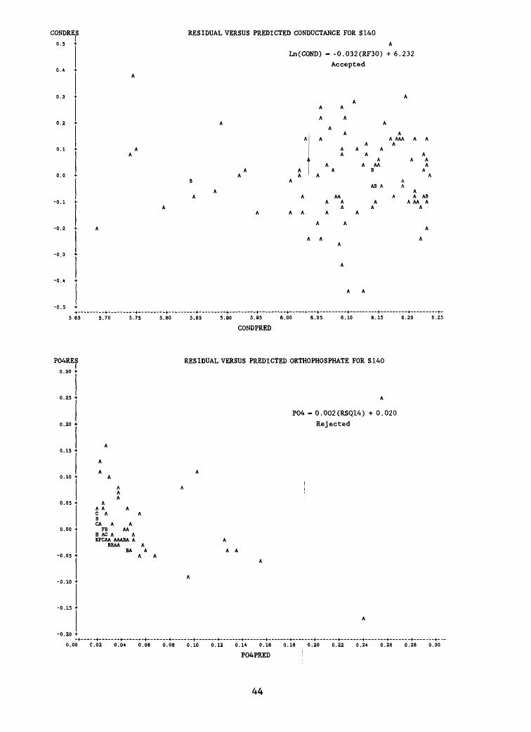
CONDRES

0.5 i

RESIDUAL VERSUS PREDICTED CONDUCTANCE FOR S140

A

Ln(COND) - -0.032(RF30) +6.232

Accepted

A A

A A

A

A A

A

A

A A

A A A A A

AA AA

B

AS A

A AAA A A A

AA A

AA

AAA A

A A

A

A A

AA AS

A AA A A

5,65 5.70 5.75 5.80 5.85 5.90 5.95

CONDPRED

6.00 6.05 6.10 6.15 6.20

P04RES0.30

A A A

AA A C A B CA A

FBH AC A A KFCAA AAABA A

BBAA A BA A

A

AA

RESIDUAL VERSUS PREDICTED ORTHOPHOSPHATE FOR S140

P04 - 0.002(RSQ14) +0.020

Rejected

0.00 C.02 0.0* 0.06 0.08 0.10 0.12 0.14 0.16 0.18 0.20 0.22 0.2* 0.26 0.28 0.30

P04PRED I

44

CONDRES

600 +

RESIDUAL VERSUS PREDICTED CONDUCTANCE FOR S7

COND - -3.139(RSQ7) +1,198.54

Rejected

Outliers removed

AAABAA

A E AACAA

AAE AB

C A

AABD AAA

AB

AA A

A

A A

500 550 600 650 700 750 800 850 900 950 1000 1050 1100 1150 1200 1250

CONDPRED

P04RES

0.40 +

0.20

B A A

AD B A CA A

ECFA M N A QE

B A

AA

-0.10 +-+—————+———————+-_

0.00 0.05 0.10

RESIDUAL VERSUS PREDICTED ORTHOPHOSPHATE FOR S7

P04 - 0.002(RSQ7) + 0.034

Rejected

0.15 0.20 0.30

P04PRED

0.50

45

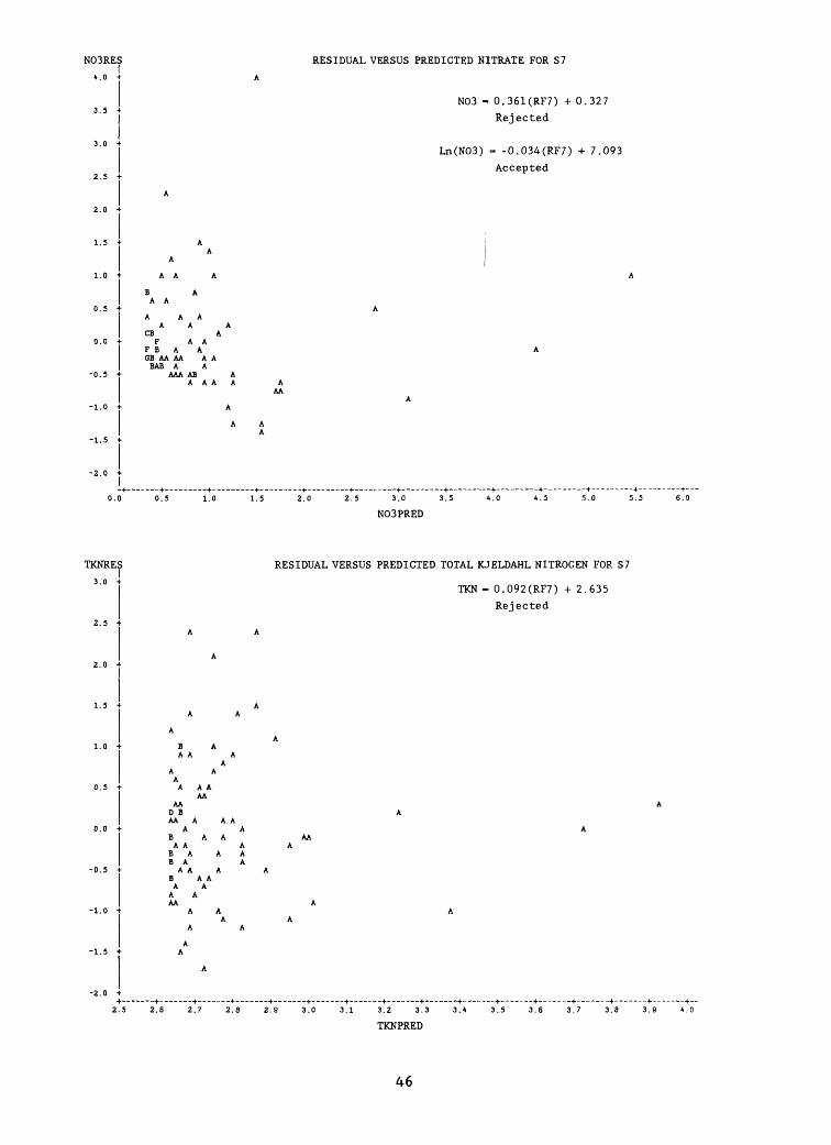
N03RES

4.0 +

RESIDUAL VERSUS PREDICTED NITRATE FOR S7

N03 - 0.361(RF7) + 0.327

Rejected

Ln(N03) - -0.034(RF7) + 7.093

Accepted

A

A A

A A

A A AA A A

CB AF A A

F B A A GB AA AA A A

BAB A AAAA AB A

A A A A A AA

A A A

2.5 3.0 3.5

N03PRED

TKNRES

3.0

RESIDUAL VERSUS PREDICTED TOTAL KJELDAHL NITROGEN FOR S7

TKN - 0.092(RF7) + 2.635

Rejected

B A A

A A AAA

AA D B AA A

A A B A A

A A

A A B A B A

A A B A A

A A A A AA

A

2.6 2.7 2.8 2.9 3.0 3.1 3.2 3.3 3.4 3.5 3.6 3.7 3.8 3.9 4.0

TKNPRED

46

TNRESI

5 +

RESIDUAL VERSUS PREDICTED TOTAL NITROGEN FOR S7 A

TN - 0.462(RF7) + 3.011

Accepted

A A A

AA

AAA A A A A A A B A A A 4 fl A A

BA AABC A A ABA A A B B A A

BA B A

2.0 2.5 3.0 3.5 *.0 4.5 5.0 5.5 6.0

TNPRED

5.5 7.0 7.5 8.0 8.5 9.0 9.5

CONDRESI

0.7 +

RESIDUAL VERSUS PREDICTED CONDUCTANCE FOR SUB

0.5

0.4 +

0.3

0.2

0.1

0.0 +

|-0.1 +

-0.2 +

-0.3 +

-0.4

-0.5

-0.6

-0.7

-0.8

-0.9 ••

Ln(COND) - -0.068(RF7) +6.95

Rejected

Ln(COND) - -0.056(RF7) + 6.94

Accepted

Outliers removed

AA AAA

AA ABAB A

A AA AE A A A

A A A A

6.33 6.39 6.51 6.57 6.63 6.87

CONDPRED

47

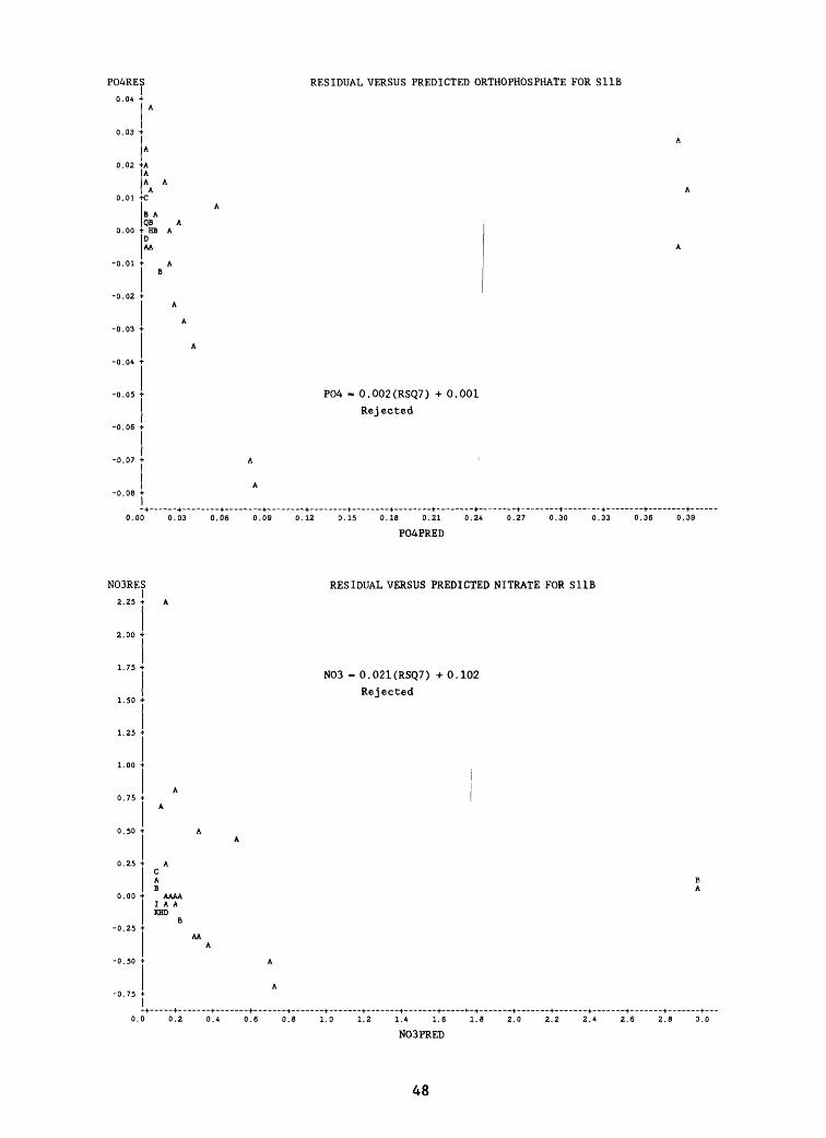
P04RES

o.o* +

0.02 +A AA A

A0.01 C

B AQB A

0.00 HB A D AA

-0.01 A

RESIDUAL VERSUS PREDICTED ORTHOPHOSPHATE FOR SUB

-0.07 -t-

-0.08 I

0.00

P04 - 0.002(RSQ7) + 0.001

Rejected

0.03 0.06 0.09 0.12 0.15 0.18 0.21 0.2A 0.27 0.30 0.33 0.36 0.39

P04PRED

N03RES

2.25 + A

AC A B

AAAA I A A KHD

B

RESIDUAL VERSUS PREDICTED NITRATE FOR SUB

N03 - 0.021(RSQ7) +0.102

Rejected

0.0 0.2 O.A 0.6 0.8 1.0 1.2 l.A 1.6 1.1

N03PRED2.0 2.2 2.A 2.6 2.8 3.0

48

TNRES RESIDUAL VERSUS PREDICTED TOTAL NITROGEN FOR SUB

TN - 0.021(RSQ7) + 2.627

Accepted

ABA

A

CBA

BAAA

AB AA A

BAAD

B A

-2.0 +

2.5 2.7 2.9 3.1 3.3 3.5 3.7 3.9 4.1 4.3 4.5 4.7 4.9 5.1 5.3 5.5

TNPRED

CONDRES

0.15 +

RESIDUAL VERSUS PREDICTED CONDUCTANCE FOR S9

A

Outlier removed

Ln(COND) - -0.034(RF7) + 6.776 Rejected

Ln(COND) - -0.027(RF7) +6.771 Accepted

-0.25 + I

A A A A

A A A A A

A A AB B A AAA

A AA AMD A B

A A AC A A B

A AA CD

ABAAAA

A A C A

AA

A AB B A AA

6.30 6.34 6.38 6.42 6.46 6.50 6.54 6.58 6.62 6.66 6.70

CONDPRED6.74 6.78

49

P04RES0.0150 +

0.0000

0.0025 + C A A F AA D

ZA SAE

E

AA

A A

-0.0100_t—————t— — ————4.—

0.00 0.01 0.02

RESIDUAL VERSUS PREDICTED ORTHOPHOSPHATE FOR S9

P04 - 0.001(RSQ7) +0.004

Accepted

0.05

P04PRED

0.08

N03RES RESIDUAL VERSUS PREDICTED NITRATE FOR S9

A A A AA

A A A AB A

A A A A UFDA A

CFB A A FBA

CCAA A AA

AAAA A

A A

N03 - 0.025(RF7) +0.007

Rejected

-4-0.00 0.03 0.06 0.09 0.12 0.15 0.18 0.21 0.^4 0.27 0.30 0.33 0.36 0.39

N03PRED

50

P04RES

0.040 +

0.035 •

AA

A A

AA

B A A A

A AMTGBGECA A CA ACB A AA

RESIDUAL VERSUS PREDICTED ORTHOPHOSPHATE FOR S151

P04 - 9.275(RSQ14) +0.005

Accepted

0.005 0.006 0.007 0.008 0.009 0.010 0.011 0.012 0.013 0.014 0.015 0.016 0.017

P04PRED

CONDRES

500 +

RESIDUAL VERSUS PREDICTED CONDUCTANCE FOR S12D

COND - -2.260(RSQ14) + 691.82

Rejected

AA

A AA B

BBABBA

B AAB A A

A B AAE

AACAAD

DAAA BD

ABA AA BB

AA A

A A AA

D

A AA

B A

A AC B

-500 ++_— -+____+_._—+____+ ._—+____+___...,._— _+——+_ — _+.___+..._+____+_ — _+_ — _+—_.+._—+——+. — .+——_+_——+———+_ — _+_——+_

220 240 260 280 300 320 340 360 380 400 420 440 460 480 500 520 540 560 580 600 620 640 660 680 700

CONDPRED

Outlier removed

51

P04RES

0.050

0.045

-0.005 •

-0.010

|0.003C

RESIDUAL VERSUS PREDICTED ORTHOPHOSPHATE FOR S12DA

P04 - 0.001(RF14) +0.003

Rejected

A AQCFBCBCEFCDA BEE BDCAC AACCBB

A A

A A A B

0.0075

P04PRED

0.0111 0.0120

CONDRED

300

RESIDUAL VERSUS PREDICTED CONDUCTANCE FOR S12A

A

COND - -23.318(L,nRF30) + 326.73

Accepted

A

A A AAA A A

BAAA A A BA AA A A

A A AA AA AAA A A B A AB

A A A A A A A

AAA AA

A

200 210 220 230 240 250 260 270 280 290 300 310 320 330 340 350 360 370 380 390 400 410 420 430 440

CONDPRED

52