Analysis of the dynamic stiffness of a soil-pile system ...Analysis of the dynamic stiffness of a soil-pile system using Abaqus Master of Science Thesis in the Master’s Programme

Analysis of the dynamic stiffness

of a soil-pile system using Abaqus Master of Science Thesis in the Master’s Programme Geo and Water Engineering

DAVID RUDEBECK Department of Civil and Environmental Engineering Division of GeoEngineering

Geotechnical Engineering Research Group

CHALMERS UNIVERSITY OF TECHNOLOGY Göteborg, Sweden 2010 Master’s Thesis 2010:125

MASTER’S THESIS 2010:125

Analysis of the dynamic stiffness

of a soil-pile system using Abaqus

Master of Science Thesis in the Master’s Programme Geo and Water Engineering

DAVID RUDEBECK

Department of Civil and Environmental Engineering Division of GeoEngineering

Geotechnical Engineering Research Group CHALMERS UNIVERSITY OF TECHNOLOGY

Göteborg, Sweden 2010

Analysis of the dynamic stiffness of a soil-pile system using Abaqus Master of Science Thesis in the Master’s Programme Geo and Water Engineering DAVID RUDEBECK

© DAVID RUDEBECK, 2010

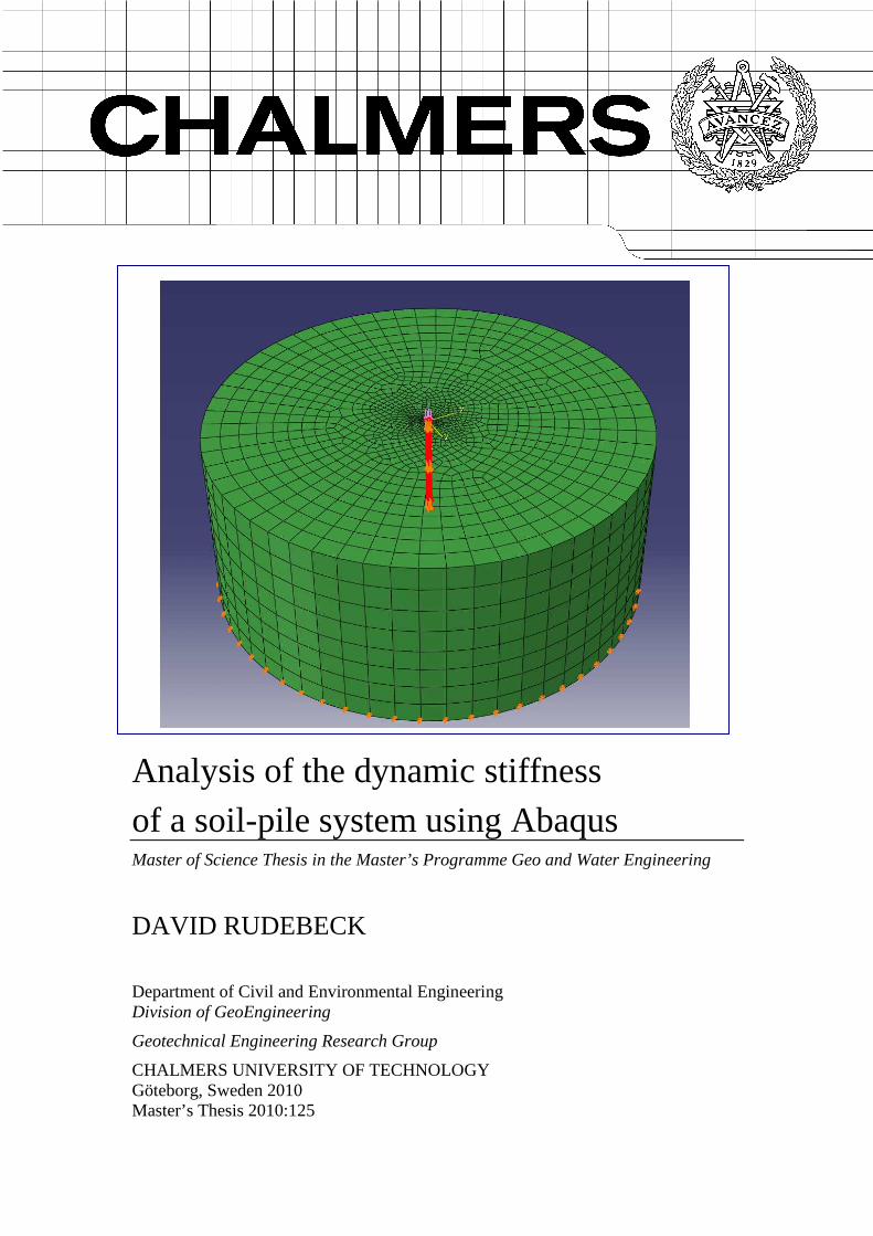
Examensarbete / Institutionen för bygg- och miljöteknik, Chalmers tekniska högskola 2010:125 Department of Civil and Environmental Engineering Division of GeoEngineering Geotechnical Engineering Research Group Chalmers University of Technology SE-412 96 Göteborg Sweden Telephone: + 46 (0)31-772 1000 Cover: Illustration of an Abaqus model simulating the response of a dynamically loaded 2x2 pile group Chalmers Reproservice Göteborg, Sweden 2010:125

I

II

Analysis of the dynamic stiffness of a soil-pile system using Abaqus Master of Science Thesis in the Master’s Programme Geo and Water Engineering DAVID RUDEBECK Department of Civil and Environmental Engineering Division of GeoEngineering Geotechnical Engineering Research Group Chalmers University of Technology

ABSTRACT

The football stadium of Gamla Ullevi was built and opened in 2009. The arena is established on 55-85 metres of clay with cohesion piles reaching a depth of 44 metres. Jumping audiences at football games resulted in soil bound vibrations bringing surrounding buildings into motion. This has brought an interest in the field of geo dynamics. The objective of this thesis is to study the soil-pile interaction of a foundation subjected to a dynamic load. As a basis for the analysis, the soil has been assumed to be linear elastic and the loading is described as harmonic. For the analysis FE models have been developed in Abaqus to simulate a vertical cyclic load of 5 kN at the head of each cohesion pile. A pile load of 5 kN is in the range of the dynamic load caused by a jumping audience at Gamla Ullevi. The amplitude of vertical displacement of the pile head as a function of the loading frequency is set as output of the model. The frequency was varied between 0-10 Hz, measured frequencies at the stadium where close to 2 Hz. From this the soil-pile stiffness could be obtained. Results from the model are verified by comparison with a response curve for a damped harmonic oscillator. Also comparisons between a single pile and a pile group are made and the dynamic response is also compared with the static case. Furthermore, a study has been carried out to determine to what extent variations in soil depth affect the soil-pile response. The study has indicated that the horizontal surroundings of the pile have greater impact on the soil-pile stiffness than the vertical surroundings, which represents the distance to the bedrock.

Key words: Abaqus, Complex-harmonic analysis, Dynamic response, Linear elastic model, Soil-pile system.

III

Analys av den dynamiska styvheten i ett jord-pålsystem användandes Abaqus Examensarbete inom Geo and Water Engineering DAVID RUDEBECK Institutionen för bygg- och miljöteknik Avdelningen för Geologi och geoteknik Forskningsgruppen för Teknisk geologi och Geoteknik Chalmers tekniska högskola

SAMMANFATTNING

Fotbollsarenan Gamla Ullevi stod klar för invigning 2009. Anläggningen grundlades på ett 55-85 meter mäktigt lerlager på kohesionspålar till ett djup av 44 meter. Kort därefter framkom det att hoppande publik vid fotbollsmatcher orsakade markbundna vibrationer som framkallade svängningar i kringliggande byggnader. Detta har aktualiserat ämnet geodynamik. Denna examensrapport syftar till att studera interaktionen jord-påle i en grund som utsätts för en dynamisk last. En parameterstudie har utförts för att bestämma på vilket sätt det vertikala avståndet mellan kohesionpåle och berggrund påverkar den dynamiska jord-pålestyvheten. Två grundläggande antaganden för analysen var att beskriva jorden som linjärelastisk och att lasten appliceras harmoniskt. I studien har finita elementmodeller utvecklats i mjukvaran Abaqus i syfte att simulera en vertikal cyklisk last på 5 kN på toppen av en kohesionspåle. Pållasten ligger inom spannet för den dynamiska lasten som en hoppande publik på Gamla Ullevi orsakar. Som output från modellen anges deflektionens amplitud som funktion av lastfrekvensen. Denna varierar mellan 0 – 10 Hz, uppmätta värden från arenan visade att hoppfrekvensen låg nära 2 Hz. Med hjälp av storleken på lasten och deflektionen kan den dynamiska styvheten för jord-pålesystemet beräknas. Resultatet från modellen har jämförts med en responskurva för en dämpad harmonisk oscillator. Jämförelser har gjorts mellan en enskild påle och en pålgrupp. På liknande sätt har jämförelser gjorts mellan den dynamiska och den statiska responsen. Vidare har en studie utförts för att studera på vilket sätt avståndet mellan påle och berggrund påverkar den dynamiska jord-pålestyvheten. Studien indikerade att utformningen av den horisontella omgivningen har större påverkan på jord-pålestyvheten än den vertikala omgivningen, dvs. avståndet till berggrunden.

Nyckelord: Abaqus, komplex harmonisk analys, dynamisk respons, linejärelastisk model, jord-pålesystem.

CHALMERS, Civil and Environmental Engineering, Master’s Thesis 2010:125 IV

Contents ABSTRACT II

SAMMANFATTNING III

CONTENTS IV

ACKNOWLEDGEMENTS VI

NOTATIONS AND ABBREVIATIONS VII

1 INTRODUCTION 1

1.1 Background 1

1.2 Objective 1

1.3 Delimitations 1

1.4 Methodology 2

2 SITE CHARACTERIZATION 3

2.1 Field tests 4

2.2 Laboratory tests 5

3 DYNAMICS OF A SOIL-PILE SYSTEM 6

3.1 Linear elastic soil model 6

3.2 Basic Equation of Dynamic Behavior 6

3.3 Dynamic stiffness functions 7

3.4 Modelling of soil properties 7

3.4.1 Poisson’s ratio 8

3.4.2 Cohesion 8

3.4.3 Isotropy 8

3.4.4 Elastic modulus 8

3.5 Wave motions 9

3.5.1 Pressure wave 9

3.5.2 Shear wave 10

3.5.3 Rayleigh wave 11

3.6 Damping 11

3.6.1 Material damping 11

3.6.2 Geometrical damping 13

3.6.3 Permeability 14

3.6.4 Non-reflecting boundaries 14

3.6.5 Nodal damping 15

3.6.6 Damped harmonic oscillator response curve 16

4 ANALYSIS USING ABAQUS 17

4.1 FEM in general 17

CHALMERS Civil and Environmental Engineering, Master’s Thesis 2010:125 V

4.2 Model development 17

4.2.1 Defining the model geometry 17

4.2.2 Assigning material properties 19

4.2.3 Assigning interaction properties 19

4.2.4 Applying loads and boundary conditions 20

4.2.5 Designing the mesh 20

4.3 FEM output 21

4.4 Dynamic soil-pile stiffness 24

4.5 Influence of soil depth 24

5 DISCUSSION ON RESULTS FROM ANALYSIS 27

5.1 Suggestions of further studies 28

6 CONCLUSIONS 29

REFERENCES 30

APPENDICES 32

CHALMERS, Civil and Environmental Engineering, Master’s Thesis 2010:125 VI

Preface and acknowledgements This master thesis is a project carried out at the Department of Civil and Environmental Engineering, Division of Geo Engineering, Geotechnical Engineering Research Group, Chalmers University of Technology, Sweden. Claes Alén (Chalmers University of Technology), Bernhard Gervide Eckel (Norconsult), Jimmy He (Norconsult) and Gunnar Widén (Akustikon) have been supervising the project. Examiner is Claes Alén.

The project has been initiated and financed by Norconsult which also has provided data from previous site investigations. Computer software has been provided by the Department of Civil and Environmental Engineering at Chalmers University of Technology.

The project was originally initiated as a task for two students in which the author and Petros Fekadu were appointed. Parts of the material for this report has been produced in collaboration with him. In a later part of the project the thesis was split into two separate theses due to time constraints. Hence this thesis is based on the same material as the report made by Petros but has been revised by the author to reach this final result.

I would like to thank my teacher and examiner Claes Alén for his helping contributions to the thesis. I would also like to thank the supportive people at Norconsult. Bengt Askmar and Bernhard Gervide Eckel supported in facility provision and gave constructive feedbacks. Jimmy He provided ideas and challenging geotechnical questions and Gunnar Widén contributed by giving guidance with regard to wave motions. Also, thanks to other employees at Norconsult that has offered their help during the work.

Göteborg, June 2010

David Rudebeck

CHALMERS Civil and Environmental Engineering, Master’s Thesis 2010:125 VII

Notations and Abbreviations

Roman upper case letters

A deflection amplitude

C damping matrix

D damping factor

Dc nodal damping coefficient

E elastic modulus

∆E elastic modulus difference

F force

G shear modulus

H hysteretic damping coefficient

K dynamic stiffness

M mass matrix

P pressure

R radius

X displacement

Roman lower case letters

a areas

a0 dimensionless frequency

c wave speed

c’ cohesion

cij frequency dependent damping coefficient

cp velocity of the P-wave

cs velocity of the S-wave

cu undrained shear strength

f frequency

i √�1

k dynamic stiffness

r radius

s element side area

� displacement

�� velocity

�� acceleration

CHALMERS, Civil and Environmental Engineering, Master’s Thesis 2010:125 VIII

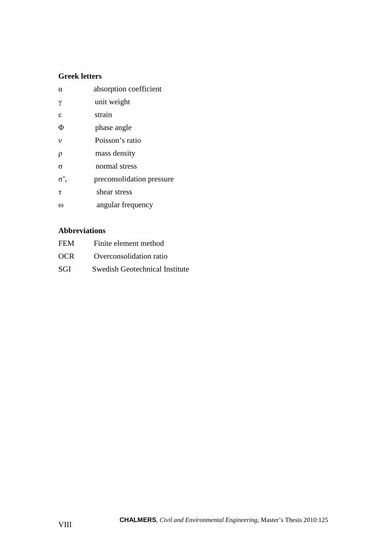
Greek letters

α absorption coefficient

γ unit weight

ε strain

Φ phase angle

ν Poisson’s ratio

ρ mass density

σ normal stress

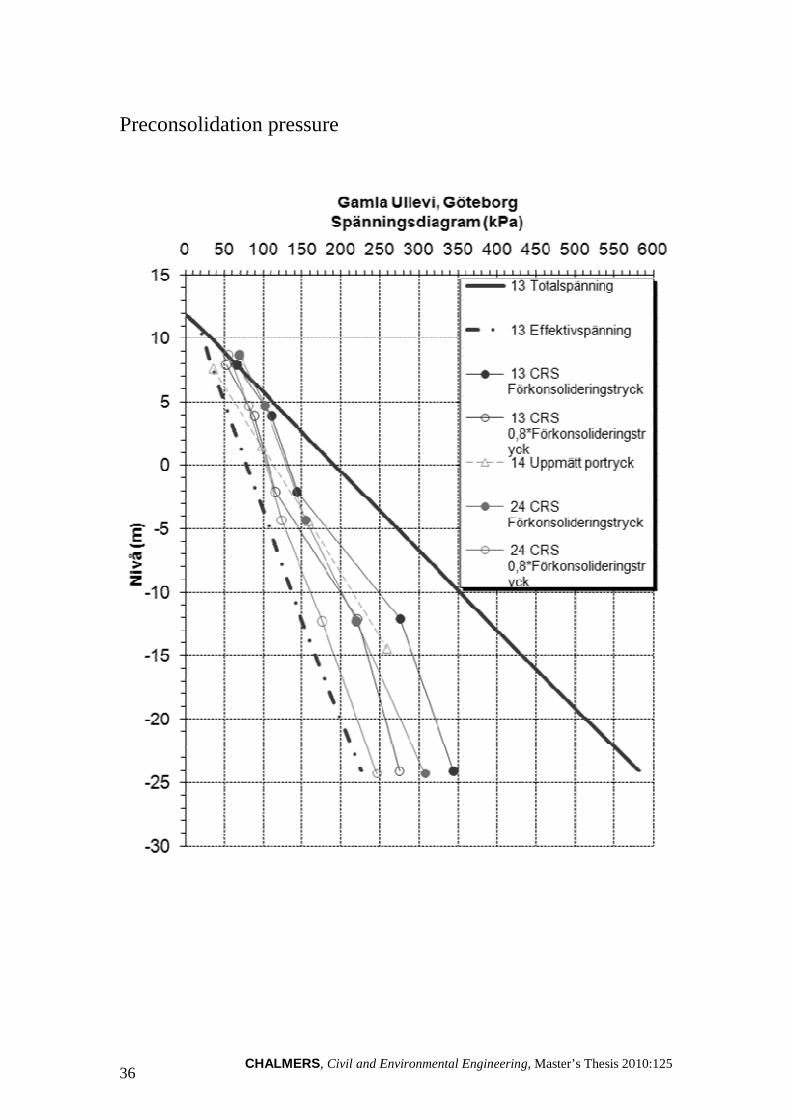
σ’ c preconsolidation pressure

τ shear stress

ω angular frequency

Abbreviations

FEM Finite element method

OCR Overconsolidation ratio

SGI Swedish Geotechnical Institute

CHALMERS, Civil and Environmental Engineering, Master’s Thesis 2010:125 1

1 Introduction

1.1 Background The phenomenon of ground vibrations in deep layers of clay has been known and experienced in Gothenburg a number of times during the last decades. In 2009 a new football stadium, Gamla Ullevi, was completed and ready for hosting domestic and international football games. In April the same year it was discovered that cyclic loadings on the standings created vibrations in the surrounding clay. Nearby buildings were exposed to horizontal vibrations up to 11.5 mm/s. This has initiated an interest in the field of soil dynamics.

Most buildings in the area, including Gamla Ullevi, are constructed on a foundation of cohesion piles. This makes them subjected to soil borne wave motions. Hence there is a need for prediction of dynamic soil-pile behaviours. Today there is little knowledge about the interaction between piles and the Gothenburg clay.

1.2 Objective The objective of this master’s thesis is to analyze the dynamic stiffness of an interacting soil-pile foundation. This is done by simulating the dynamic response of the system using complex harmonic analysis. Separate results are presented for a single pile and a pile group with input data from the construction and the soil at Gamla Ullevi. In the analysis, studies will be conducted on soil depths to determine their specific impact on the dynamic response. The results will be evaluated with harmonic oscillation response curves as references.

1.3 Delimitations The thesis focuses on predicting the dynamic stiffness of a soil-pile system considering both single pile and pile group cases. In addition, static stiffness is determined for comparison. The vertical stiffness is studied, hence inclusion of the lateral stiffness is recommended for further studies.

The location in consideration is Gamla Ullevi where the geotechnical condition is clay to depths of 55-85 meters with soil parameters varying with depth. The thesis considers concrete piles since that was used at the construction site.

In the real scenario, piles are subjected to different loading conditions such as vertical forces, horizontal forces and moments. However, the predominant component is the vertical loading in the Gamla Ullevi case. Thus, this study is limited to consider the dynamic vertical force which could reasonably represent practical situations.

Depending on the amount of stress, soil can exhibit different stress-strain behaviours such as elastic and plastic. A previous study states that plasticity is known to reduce the stiffness of the soil-pile system (Maheshwari 1997). But the study is limited to


such an elastic model with a linear case by subjecting the system to a small amplitude of cyclic loading.

Analysis of dynamic stiffness involves multidisciplinary and comprehensive procedures which may be geotechnical and non-geotechnical in nature. However, the thesis is principally concerned in analysis of the geotechnical matters, viz., the soil and the foundation.

1.4 Methodology The work encompasses numerous methods and steps to carry out the task systematically. It entails literature survey, incorporation of available data, modeling the scenario and handling of FEM software.

First, a literature survey was made to obtain general knowledge in the subject relevant to carry out the following work in the project. This included an understanding in geo dynamics and FEM software.

Site investigation data was gathered to receive all pertinent properties of the soil at the specific location. The main source of information was a report made by Gatubolaget containing a compilation of site investigations carried out in the area. The most recent investigation was done by Gatubolaget in 2006. The dynamic soil properties were then incorporated in the linear elastic soil model.

Afterwards, a realistic scenario was conceptualized and a model of the soil-pile system was produced. This was accomplished for both single pile and pile group cases and serves as a bridge between the input data and the FEM analyses. FEM results were compiled, checked for verification and analysed.

The finite element method (FEM) software Abaqus was used to analyze the problem. The models are developed and simulated in Abaqus to perform complex harmonic analyses in three dimensions. The results of the thesis are produced by the FEM analysis with 3D program modelling. From the simulation, vertical displacement values for different cases are chosen as output. The results are evaluated against harmonic oscillation response curves. Then comparisons are made and conclusions are drawn.

CHALMERS, Civil and Environmental Engineering

2 Site characterizationThe Gamla Ullevi arena is constructed on a foundation consisting of nearly 1200 cohesion piles reaching a depth of 44 meters. The the site and the framework consists of concrete columns and beams. The roof is a steel construction made by welded Iattachment. (Figure 2.1)

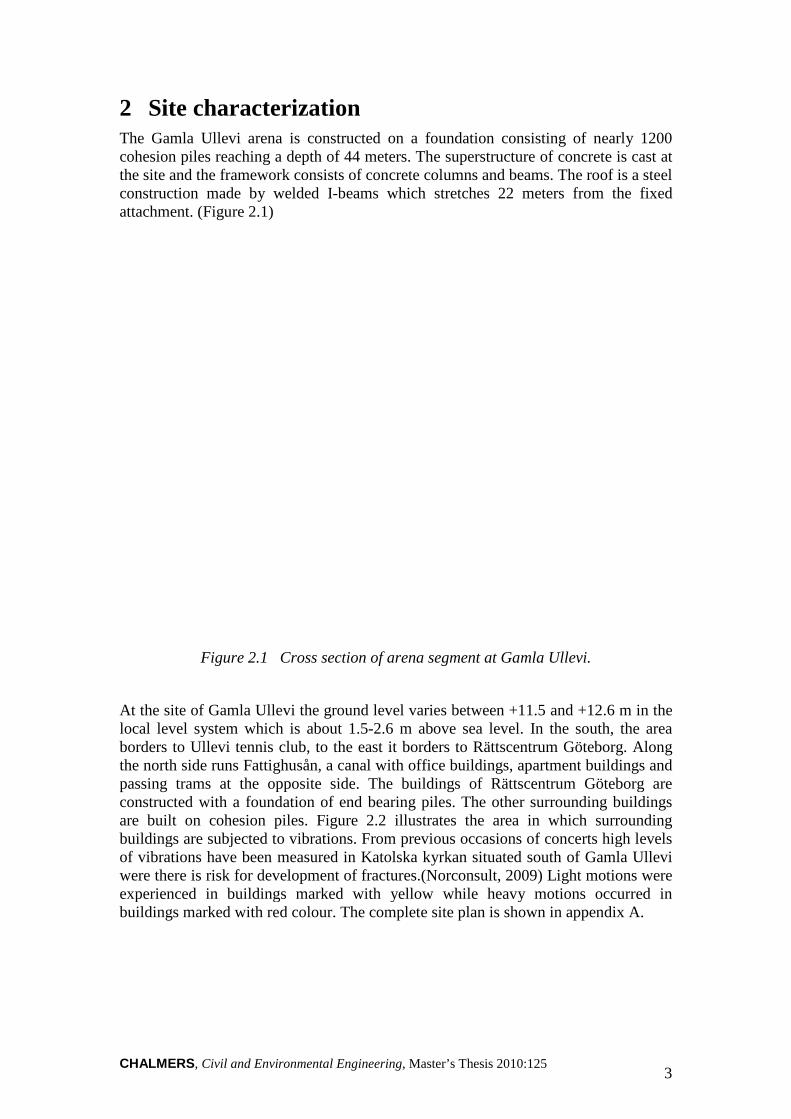
Figure 2.1 Cross section of arena segment at Gamla Ullevi.

At the site of Gamla Ullevi the ground level varies between +11.5 and +12.6 m local level system which is about 1.5borders to Ullevi tennis club, to the east it borders to Rättscentrum Göteborgthe north side runs Fattighusånpassing trams at the opposite sideconstructed with a foundation of end bearing piles. The other surrounding buildings are built on cohesion piles. buildings are subjected to vibrations. of vibrations have been measured in Katolska kyrkanwere there is risk for development of fractures.experienced in buildings marked buildings marked with red

Civil and Environmental Engineering, Master’s Thesis 2010:125

Site characterization arena is constructed on a foundation consisting of nearly 1200

piles reaching a depth of 44 meters. The superstructure of concretethe site and the framework consists of concrete columns and beams. The roof is a steel construction made by welded I-beams which stretches 22 meters from the fixed

Cross section of arena segment at Gamla Ullevi.

At the site of Gamla Ullevi the ground level varies between +11.5 and +12.6 m which is about 1.5-2.6 m above sea level. In the south, the area

borders to Ullevi tennis club, to the east it borders to Rättscentrum Göteborgruns Fattighusån, a canal with office buildings, apartment buildings and at the opposite side. The buildings of Rättscentrum Göteborg are

constructed with a foundation of end bearing piles. The other surrounding buildings cohesion piles. Figure 2.2 illustrates the area in which surrounding

buildings are subjected to vibrations. From previous occasions of concerts high levels of vibrations have been measured in Katolska kyrkan situated south of Gamla Ullevi

here is risk for development of fractures.(Norconsult, 2009) Light motions were experienced in buildings marked with yellow while heavy motions occur

red colour. The complete site plan is shown in appendix A.

3

arena is constructed on a foundation consisting of nearly 1200 superstructure of concrete is cast at

the site and the framework consists of concrete columns and beams. The roof is a steel beams which stretches 22 meters from the fixed

Cross section of arena segment at Gamla Ullevi.

At the site of Gamla Ullevi the ground level varies between +11.5 and +12.6 m in the In the south, the area

borders to Ullevi tennis club, to the east it borders to Rättscentrum Göteborg. Along with office buildings, apartment buildings and

centrum Göteborg are constructed with a foundation of end bearing piles. The other surrounding buildings

illustrates the area in which surrounding certs high levels

situated south of Gamla Ullevi Light motions were

yellow while heavy motions occurred in The complete site plan is shown in appendix A.

CHALMERS4

Figure

In a report made by Norconsult in 2009 varying depths between 52filling material and dry crust. The filling material consists of sand, gravel, stones acrushed bricks. The top 10 meters as “very soft”. (Gatubolaget, 2006)

2.1 Field tests Data from field tests have been Gatukontoret carried out tests

- Static penetration performed at- Compilation of undisturbed soil samples in - Measurements of ground water surface level from an open pipe- Compilation of disturbed soil samples using helical auger.- Seismic investigations

(Gatukontoret, 1985

A more recent investigation investigations. It was carried out by Gatubolaget on behalf of HIGAB to provide geotechnical information to

Fattighusån

Gamla Ullevi

Ullevi tennis club

Katolska kyrkan

CHALMERS, Civil and Environmental Engineering, Master’s Thesis

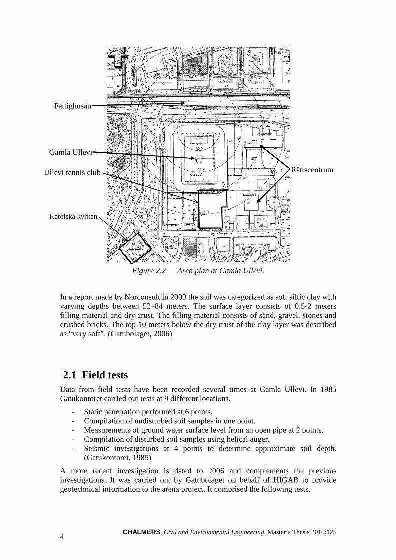
Figure 2.2 Area plan at Gamla Ullevi.

In a report made by Norconsult in 2009 the soil was categorized as soft silticvarying depths between 52–84 meters. The surface layer consists of 0.5filling material and dry crust. The filling material consists of sand, gravel, stones a

10 meters below the dry crust of the clay layer was described (Gatubolaget, 2006)

have been recorded several times at Gamla Ullevi. Gatukontoret carried out tests at 9 different locations.

performed at 6 points. Compilation of undisturbed soil samples in one point. Measurements of ground water surface level from an open pipe Compilation of disturbed soil samples using helical auger.

smic investigations at 4 points to determine approximate soil depth.(Gatukontoret, 1985)

investigation is dated to 2006 and complementsinvestigations. It was carried out by Gatubolaget on behalf of HIGAB to provide

to the arena project. It comprised the following tests.

, Master’s Thesis 2010:125

il was categorized as soft siltic clay with The surface layer consists of 0.5-2 meters

filling material and dry crust. The filling material consists of sand, gravel, stones and layer was described

several times at Gamla Ullevi. In 1985

at 2 points.

4 points to determine approximate soil depth.

and complements the previous investigations. It was carried out by Gatubolaget on behalf of HIGAB to provide

the arena project. It comprised the following tests.

Rättscentrum


- Static penetration test, performed at 3 points. - Cone penetration test, carried out at 3 points - Field vane shear test at 2 points - Pore pressure measurements by a piezometer in 4 levels at one station.

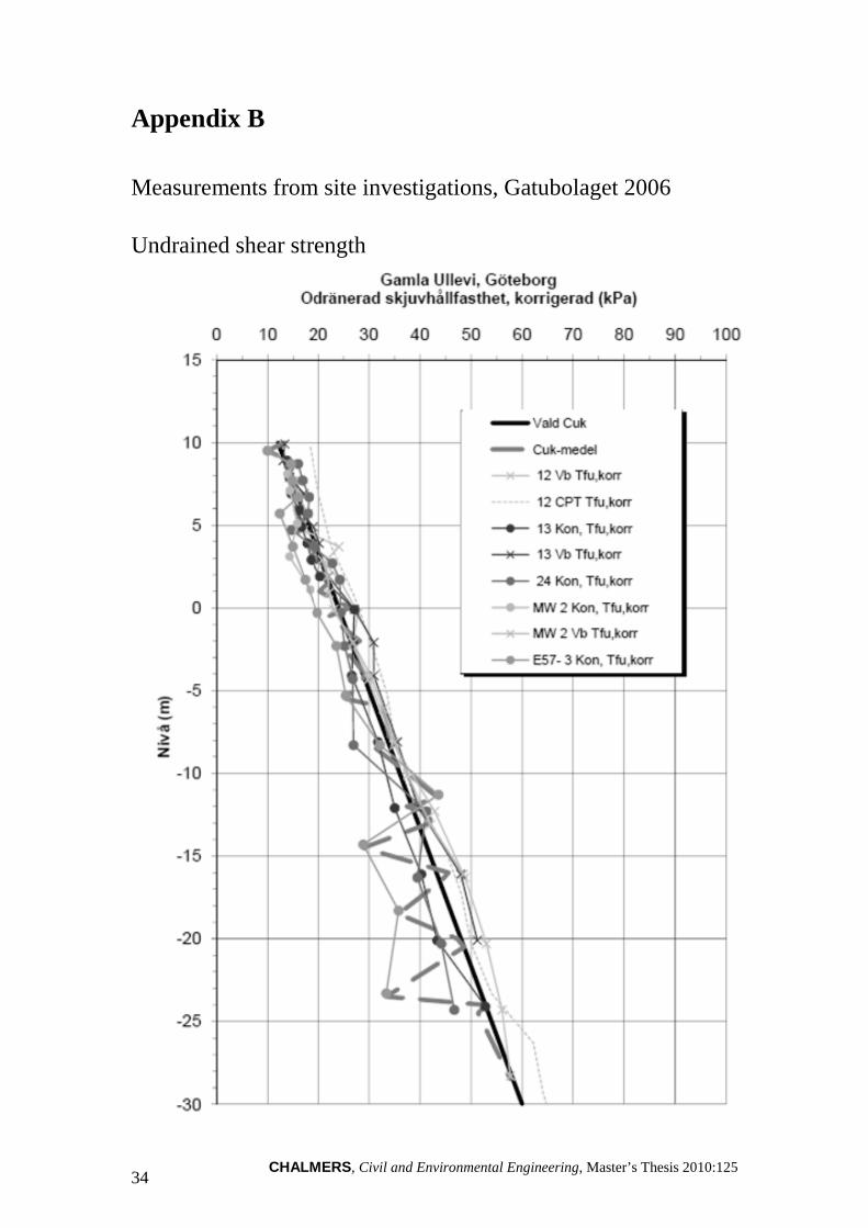
Based on the results from the site investigations a representative value for the undrained shear stress was determined to:

cu = 12 kPa at top of clay layer, increasing with depth + 1.2 kPa/m.

(Gatubolaget, 2006)

2.2 Laboratory tests In 1985 the geotechnical laboratory of the roadwork department studied a number of disturbed and undisturbed soil samples in the area of Gamla Ullevi. The disturbed samples were studied to determine the soil types.

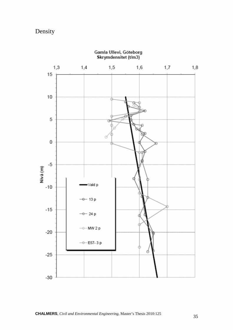
Odometer tests were carried out on samples from three depths, 10 m, 20 m, and 30 m below the ground surface. Other tests were also carried out on the undisturbed soil samples regarding density, moisture content, liquid limit, consolidation ratio (CRS), sensitivity and shear strength. A selection of the results is presented below.

- Density: 1560 – 1800 kg/m3

- Moisture content: 32 %, dry crust 45-100 %, clay 20 %, filling material.

- OCR: 1.3 - 1.9, decreasing with depth.

In addition to the geotechnical investigation, a number of analyses were carried out to determine the content of different metals and chemicals in the soil. (Gatukontoret, 1985)

Complete results of the tests are presented in graphs and tables in appendix B.


3 Dynamics of a soil-pile system If a structure´s long-term response to applied loads is sought, a static analysis has to be performed. However, if the loading has a short duration as in the cases of machine vibrations, compaction, pile driving, wave loading and earthquakes, the loading is dynamic in nature. Thus, a dynamic analysis ought to be made.

Dynamic stiffness of soil including both elastic stiffness and damping can be represented by a complex quantity of data. Thus, it needs to use software capable of running complex-harmonic analyses. In the complex data, the real part represents the spring stiffness and the imaginary part represents damping. (Maheshwari, 2005)

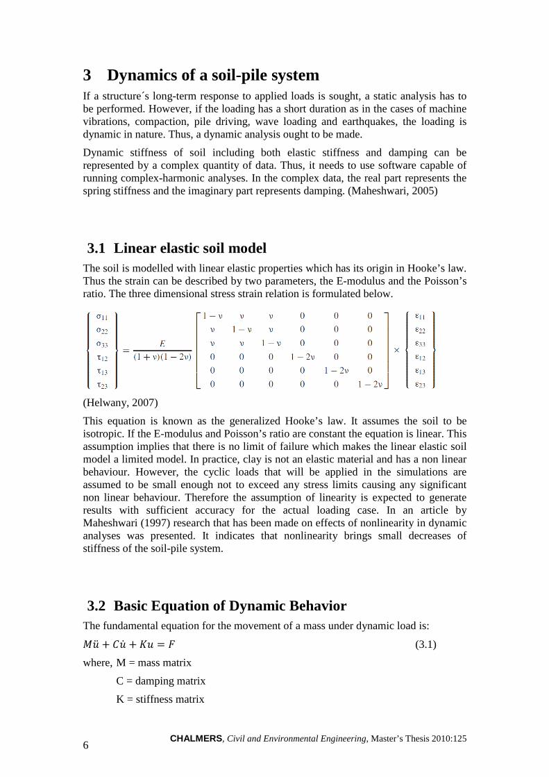
3.1 Linear elastic soil model The soil is modelled with linear elastic properties which has its origin in Hooke’s law. Thus the strain can be described by two parameters, the E-modulus and the Poisson’s ratio. The three dimensional stress strain relation is formulated below.

(Helwany, 2007)

This equation is known as the generalized Hooke’s law. It assumes the soil to be isotropic. If the E-modulus and Poisson’s ratio are constant the equation is linear. This assumption implies that there is no limit of failure which makes the linear elastic soil model a limited model. In practice, clay is not an elastic material and has a non linear behaviour. However, the cyclic loads that will be applied in the simulations are assumed to be small enough not to exceed any stress limits causing any significant non linear behaviour. Therefore the assumption of linearity is expected to generate results with sufficient accuracy for the actual loading case. In an article by Maheshwari (1997) research that has been made on effects of nonlinearity in dynamic analyses was presented. It indicates that nonlinearity brings small decreases of stiffness of the soil-pile system.

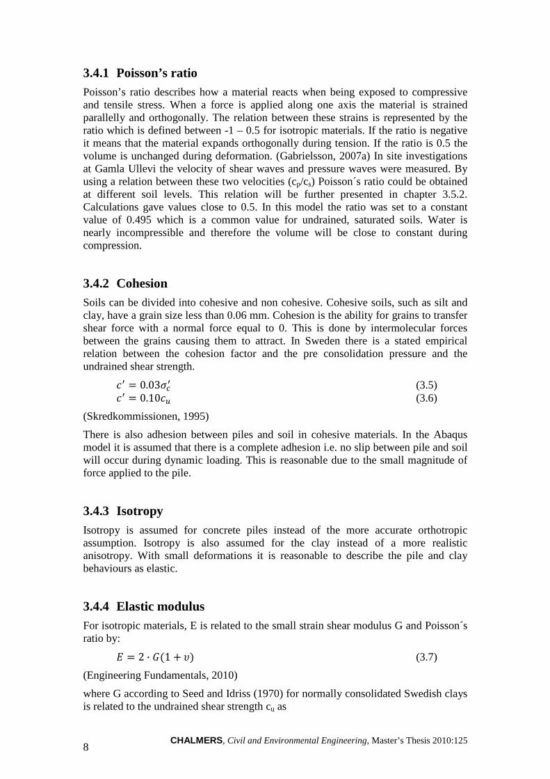
3.2 Basic Equation of Dynamic Behavior The fundamental equation for the movement of a mass under dynamic load is:

�� (3.1)

where, M = mass matrix

C = damping matrix

K = stiffness matrix


�� = acceleration

�� = velocity

� = displacement

F = applied load (Brinkgreve et.al, 2006)

The basic difference between static and dynamic analyses is the inclusion of the inertial forces �� in the equation of equilibrium. In this case the mass matrix represents the mass of the soil. Hence in a static analysis the internal forces arise only from the deformation of the structure while in a dynamic analysis the internal forces contain contributions created by both the motion and the deformation of the structure.

3.3 Dynamic stiffness functions Requested output of the FE-models is the vertical displacement of the pile head. The vertical displacement is calculated as a complex response which means that there is a phase relation between the force velocity and the particle velocity. The dynamic stiffness is then calculated as a function of the applied force and the vertical displacement of the pile head. (Ewins, 1984)

��

� (3.2)

where K = dynamic stiffness (N/m) F = force (N) X = displacement (m)

The dynamic stiffness matrix for a harmonic excitation is frequency dependent and can be written as:

�� (3.3)

where kij = frequency dependent dynamic stiffness (N/m) cij = frequency dependent damping coefficient (N/m) a0 = dimensionless frequency

The dimensionless frequency can be expressed using the following relation:

��

�� (3.4)

Where ω = angular velocity (rad/s) d = pile diameter (m) cs = soil shear wave velocity (m/s) (Maeso, Aznárez, García, 2004a)

3.4 Modelling of soil properties During the development of the FE-model a number of assumptions had to be made in order to describe the non-linear soil properties at the site in the linear model. These properties are presented below together with the assumptions made when implementing them in the model.


3.4.1 Poisson’s ratio Poisson’s ratio describes how a material reacts when being exposed to compressive and tensile stress. When a force is applied along one axis the material is strained parallelly and orthogonally. The relation between these strains is represented by the ratio which is defined between -1 – 0.5 for isotropic materials. If the ratio is negative it means that the material expands orthogonally during tension. If the ratio is 0.5 the volume is unchanged during deformation. (Gabrielsson, 2007a) In site investigations at Gamla Ullevi the velocity of shear waves and pressure waves were measured. By using a relation between these two velocities (cp/cs) Poisson´s ratio could be obtained at different soil levels. This relation will be further presented in chapter 3.5.2. Calculations gave values close to 0.5. In this model the ratio was set to a constant value of 0.495 which is a common value for undrained, saturated soils. Water is nearly incompressible and therefore the volume will be close to constant during compression.

3.4.2 Cohesion Soils can be divided into cohesive and non cohesive. Cohesive soils, such as silt and clay, have a grain size less than 0.06 mm. Cohesion is the ability for grains to transfer shear force with a normal force equal to 0. This is done by intermolecular forces between the grains causing them to attract. In Sweden there is a stated empirical relation between the cohesion factor and the pre consolidation pressure and the undrained shear strength.

�� 0.03�� (3.5)

�� 0.10� (3.6)

(Skredkommissionen, 1995)

There is also adhesion between piles and soil in cohesive materials. In the Abaqus model it is assumed that there is a complete adhesion i.e. no slip between pile and soil will occur during dynamic loading. This is reasonable due to the small magnitude of force applied to the pile.

3.4.3 Isotropy Isotropy is assumed for concrete piles instead of the more accurate orthotropic assumption. Isotropy is also assumed for the clay instead of a more realistic anisotropy. With small deformations it is reasonable to describe the pile and clay behaviours as elastic.

3.4.4 Elastic modulus For isotropic materials, E is related to the small strain shear modulus G and Poisson´s ratio by:

! � 2 · $%1 � &' (3.7)

(Engineering Fundamentals, 2010)

where G according to Seed and Idriss (1970) for normally consolidated Swedish clays is related to the undrained shear strength cu as


(

�)* 500 (3.8)

Combining (3.7) and (3.8) the elastic modulus can be expressed as

! � 1000 · %1 � &' (3.9)

As can be seen above, the estimation of the elastic modulus is based on empirical relations to the shear modulus and Poison’s ratio. The shear modulus can be estimated by field tests e.g. cone penetration test or standard penetration test (SPT).

3.5 Wave motions The definition of a wave is a motion around a state of equilibrium. In soil it can be caused by tectonic movement resulting in earth tremors or in more extreme cases, earthquakes. In this case the vibrations are caused by vertical cyclic loads on the surface that dislocates the soil particles from equilibrium. If the impact is large enough the dislocation can be permanent which densifies the soil. In the field of ground improvement the technique of dynamic compaction is a commonly used method to densify soil. The force magnitude in this case is limited to 5 kN on undrained soil. Under these circumstances no permanent dislocation of soil particles will occur.

Vibrations are commonly described as harmonic motions also referred to as sinus vibrations. ,%-' � A sin%2- � Φ' (3.10) Where x(t) = deflection (m) A = deflection amplitude (m) ω = angular frequency (rad/s) t = time (s) Φ = phase angle (rad)

In this relation a wave can be described with two parameters, amplitude and angular frequency.

There are mainly three wave types that are studied in dynamic soil tests. The pressure wave (P-wave), shear wave (S-wave) and the surface bound Rayleigh wave are described below. (Möller, Larsson, Bengtsson, Moritz. 2000)

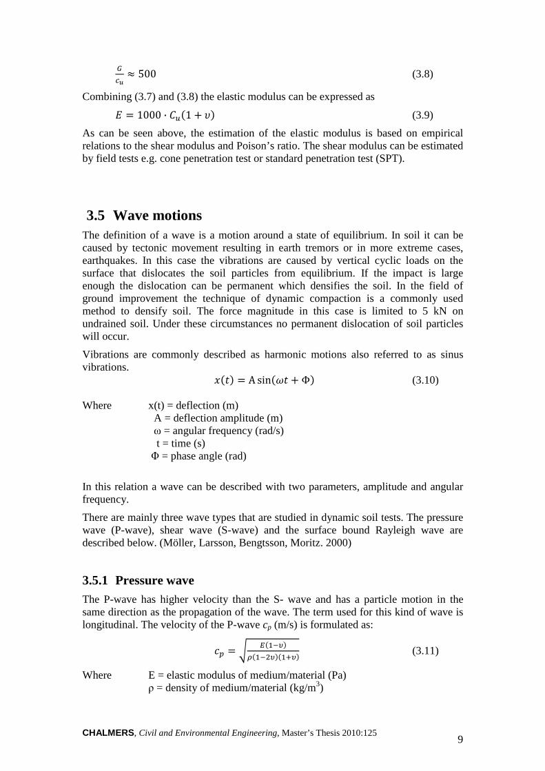
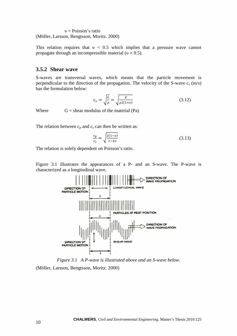
3.5.1 Pressure wave The P-wave has higher velocity than the S- wave and has a particle motion in the same direction as the propagation of the wave. The term used for this kind of wave is longitudinal. The velocity of the P-wave cp (m/s) is formulated as:

�4 � 5 6%789':%78;9'%7<9' (3.11)

Where E = elastic modulus of medium/material (Pa) ρ = density of medium/material (kg/m3)


υ = Poisson’s ratio (Möller, Larsson, Bengtsson, Moritz. 2000) This relation requires that υ < 0.5 which implies that a pressure wave cannot propagate through an incompressible material (υ = 0.5).

3.5.2 Shear wave S-waves are transversal waves, which means that the particle movement is perpendicular to the direction of the propagation. The velocity of the S-wave cs (m/s) has the formulation below:

�= � 5(: � 5 6

:;%7<9' (3.12)

Where G = shear modulus of the material (Pa)

The relation between cp and cs can then be written as:

�>�� 5;%789'

78;9 (3.13)

The relation is solely dependent on Poisson’s ratio.

Figure 3.1 illustrates the appearances of a P- and an S-wave. The P-wave is characterized as a longitudinal wave.

Figure 3.1 A P-wave is illustrated above and an S-wave below.

(Möller, Larsson, Bengtsson, Moritz. 2000)


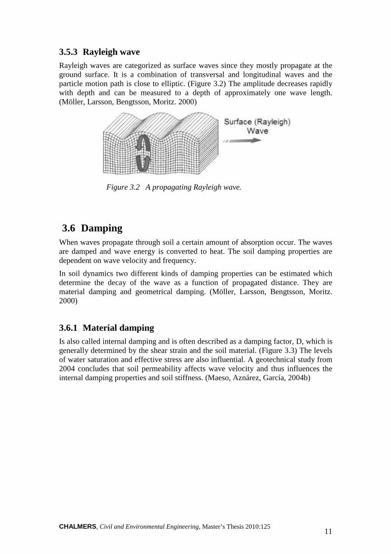
3.5.3 Rayleigh wave Rayleigh waves are categorized as surface ground surface. It is a combination ofparticle motion path is close to elliptic.with depth and can be measured to a depth of (Möller, Larsson, Bengtsson, Moritz. 2000

Figure 3.2

3.6 Damping When waves propagate through soil a certain amount of absorption occur. The waves are damped and wave energy is converted to dependent on wave velocity and frequency.

In soil dynamics two different kinds of damping properties can be estimated which determine the decay of the wave material damping and geometrical damping. 2000)

3.6.1 Material dampingIs also called internal damping and is often described as a damping factor, D, which is generally determined by the shear strain and the soil materialof water saturation and effective stress are also influential. 2004 concludes that soil permeability affects wave velocity and thus influenceinternal damping properties and soil stiffness.


Rayleigh waves are categorized as surface waves since they mostly propagate at the

urface. It is a combination of transversal and longitudinal waveparticle motion path is close to elliptic. (Figure 3.2) The amplitude decreases rapidly with depth and can be measured to a depth of approximately one wave lengt

, Larsson, Bengtsson, Moritz. 2000)

A propagating Rayleigh wave.

When waves propagate through soil a certain amount of absorption occur. The waves are damped and wave energy is converted to heat. The soil damping properties are

wave velocity and frequency.

In soil dynamics two different kinds of damping properties can be estimated which determine the decay of the wave as a function of propagated distance. They are

ng and geometrical damping. (Möller, Larsson, Bengtsson, Moritz.

Material damping Is also called internal damping and is often described as a damping factor, D, which is

determined by the shear strain and the soil material. (Figure of water saturation and effective stress are also influential. A geotechnical study from

soil permeability affects wave velocity and thus influenceinternal damping properties and soil stiffness. (Maeso, Aznárez, García,

11

waves since they mostly propagate at the transversal and longitudinal waves and the

The amplitude decreases rapidly one wave length.

When waves propagate through soil a certain amount of absorption occur. The waves ping properties are

In soil dynamics two different kinds of damping properties can be estimated which distance. They are

, Larsson, Bengtsson, Moritz.

Is also called internal damping and is often described as a damping factor, D, which is . (Figure 3.3) The levels

A geotechnical study from soil permeability affects wave velocity and thus influences the

García, 2004b)


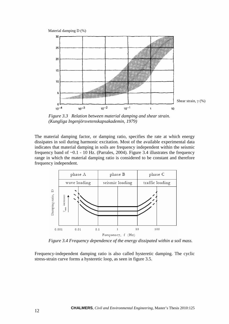
Figure 3.3 Relation between material damping and shear strain. (Kungliga Ingenjörsvetenskapsakademin, 1979)

The material damping factor, or damping ratio, specifies the rate at which energy dissipates in soil during harmonic excitation. Most of the available experimental data indicates that material damping in soils are frequency independent within the seismic frequency band of ~0.1 - 10 Hz. (Parrales, 2004). Figure 3.4 illustrates the frequency range in which the material damping ratio is considered to be constant and therefore frequency independent.

Figure 3.4 Frequency dependence of the energy dissipated within a soil mass.

Frequency-independent damping ratio is also called hysteretic damping. The cyclic stress-strain curve forms a hysteretic loop, as seen in figure 3.5.

Material damping D (%)

Shear strain, γ (%)


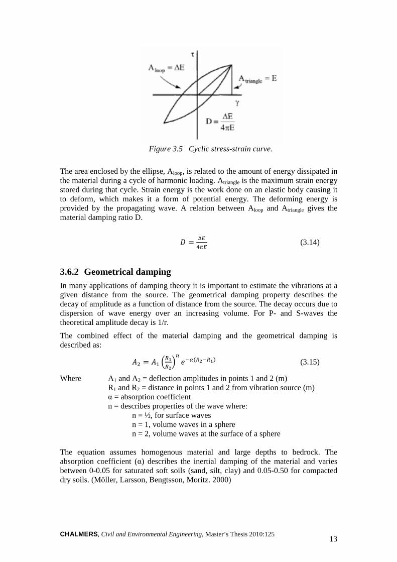
Figure 3.5 Cyclic stress-strain curve.

The area enclosed by the ellipse, Aloop, is related to the amount of energy dissipated in the material during a cycle of harmonic loading. Atriangle is the maximum strain energy stored during that cycle. Strain energy is the work done on an elastic body causing it to deform, which makes it a form of potential energy. The deforming energy is provided by the propagating wave. A relation between Aloop and Atriangle gives the material damping ratio D.

? � ∆6AB6 (3.14)

3.6.2 Geometrical damping In many applications of damping theory it is important to estimate the vibrations at a given distance from the source. The geometrical damping property describes the decay of amplitude as a function of distance from the source. The decay occurs due to dispersion of wave energy over an increasing volume. For P- and S-waves the theoretical amplitude decay is 1/r.

The combined effect of the material damping and the geometrical damping is described as:

C; � C7 DEFEGHI J8K%EG8EF' (3.15)

Where A1 and A2 = deflection amplitudes in points 1 and 2 (m) R1 and R2 = distance in points 1 and 2 from vibration source (m) α = absorption coefficient

n = describes properties of the wave where: n = ½, for surface waves

n = 1, volume waves in a sphere n = 2, volume waves at the surface of a sphere The equation assumes homogenous material and large depths to bedrock. The absorption coefficient (α) describes the inertial damping of the material and varies between 0-0.05 for saturated soft soils (sand, silt, clay) and 0.05-0.50 for compacted dry soils. (Möller, Larsson, Bengtsson, Moritz. 2000)


3.6.3 Permeability In an article written by Maeso, Aznárez and Garcis (2004c) the dynamic stiffness coefficients were computed by constructing a three-dimensional boundary element model. They found that the dissipation constant b, which is inversely proportional to the permeability k, affects the dynamic response significantly. High values of b imply greater difficulty in the fluid transit through the solid skeleton compared to low values of b. High values are obtained in clays and low values in loose sands.

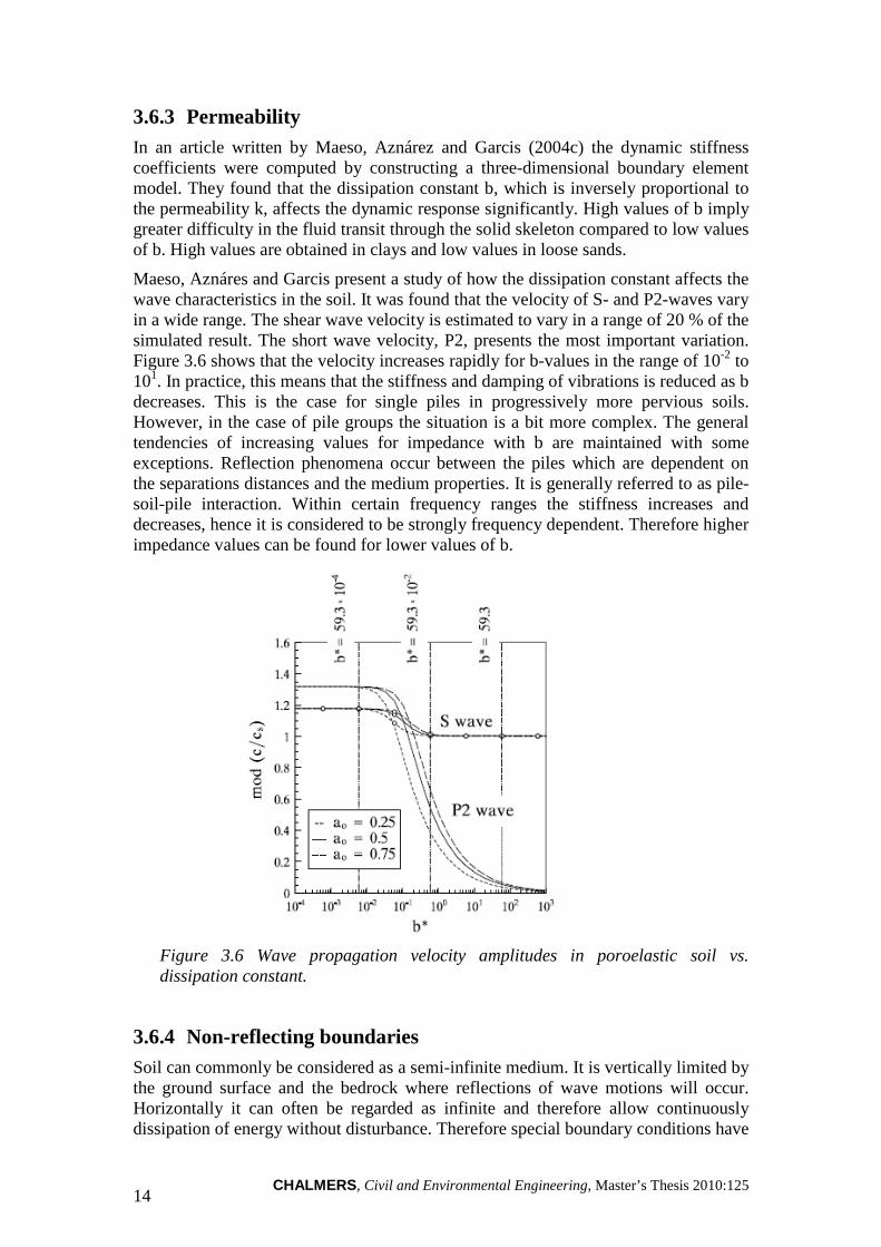
Maeso, Aznáres and Garcis present a study of how the dissipation constant affects the wave characteristics in the soil. It was found that the velocity of S- and P2-waves vary in a wide range. The shear wave velocity is estimated to vary in a range of 20 % of the simulated result. The short wave velocity, P2, presents the most important variation. Figure 3.6 shows that the velocity increases rapidly for b-values in the range of 10-2 to 101. In practice, this means that the stiffness and damping of vibrations is reduced as b decreases. This is the case for single piles in progressively more pervious soils. However, in the case of pile groups the situation is a bit more complex. The general tendencies of increasing values for impedance with b are maintained with some exceptions. Reflection phenomena occur between the piles which are dependent on the separations distances and the medium properties. It is generally referred to as pile-soil-pile interaction. Within certain frequency ranges the stiffness increases and decreases, hence it is considered to be strongly frequency dependent. Therefore higher impedance values can be found for lower values of b.

Figure 3.6 Wave propagation velocity amplitudes in poroelastic soil vs. dissipation constant.

3.6.4 Non-reflecting boundaries Soil can commonly be considered as a semi-infinite medium. It is vertically limited by the ground surface and the bedrock where reflections of wave motions will occur. Horizontally it can often be regarded as infinite and therefore allow continuously dissipation of energy without disturbance. Therefore special boundary conditions have


been defined in the outer surface nodes to counteract reflections in the FE-model. The reflections would otherwise disturb the result of the deflection amplitude of the wave motions. A further description of the non-reflecting boundaries is presented below.

3.6.5 Nodal damping As previously stated, damping of the outer nodes is arranged to prevent reflections from the horizontal surface of the soil model. Thereby an amplitude can be obtained that is undisturbed by reflected horizontal waves. Calculation of the nodal damping coefficient is based on the theory of equilibrium between the soil wave force and the damping force. The nodal damping coefficient is specified as force per velocity (N/(m/s)) where the velocity is the relative motion between two nodes. (Abaqus manual, 2010)

� � 56: (3.16)

CI � =

; (3.17)

� CIL� (3.18) Where c = wave speed (m/s) E = elastic modulus (Pa) ρ = density (kg/m3) s = element side area (m2) An = node area (m2) C = nodal damping coefficient (N/(m/s))

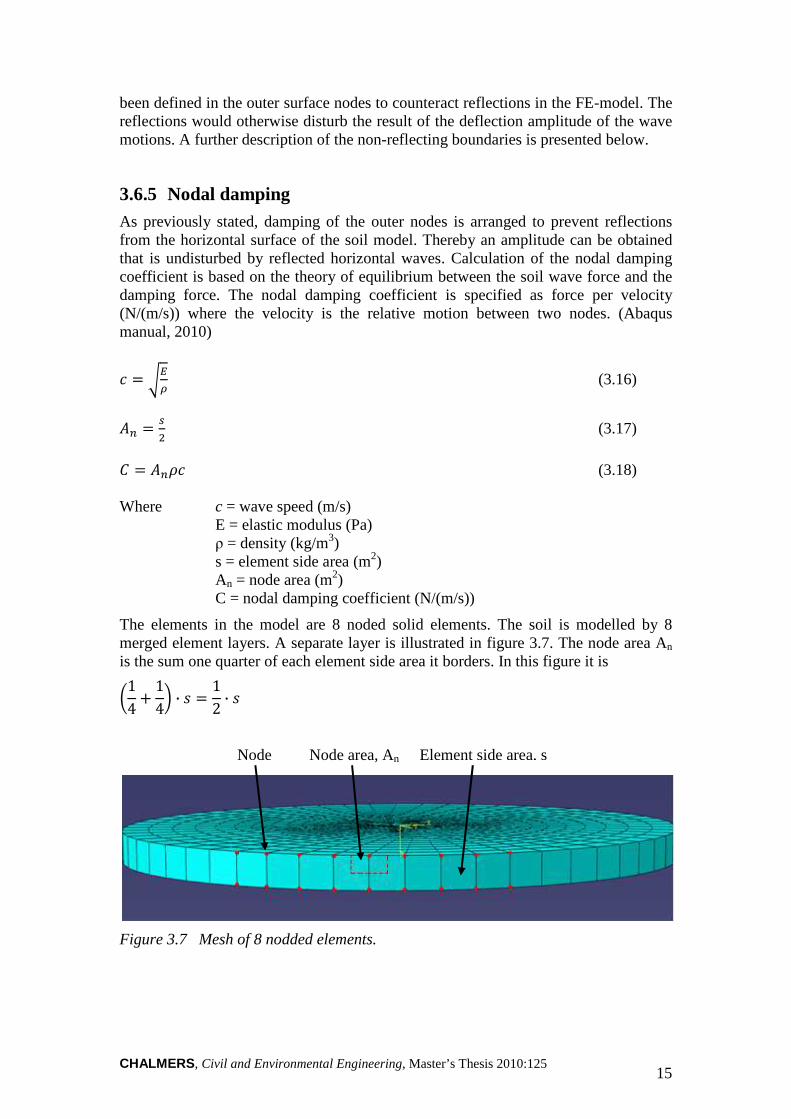
The elements in the model are 8 noded solid elements. The soil is modelled by 8 merged element layers. A separate layer is illustrated in figure 3.7. The node area An is the sum one quarter of each element side area it borders. In this figure it is

M14 � 1

4O · P � 12 · P

Figure 3.7 Mesh of 8 nodded elements.

Node area, An Node Element side area, s

CHALMERS16

3.6.6 Damped harmonic oscillatorAs previously stated, the soilThis makes it possible to describe it as a system of springs and dampers subjected to a vertical force. Figure 3.8 dynamic response of this damped harmonic oscillator3.9. At a frequency of 0 Hz the load is static. The dynamic response is normalized against the static response. by the static displacement. The xeigenfrequency of the system. D, or D

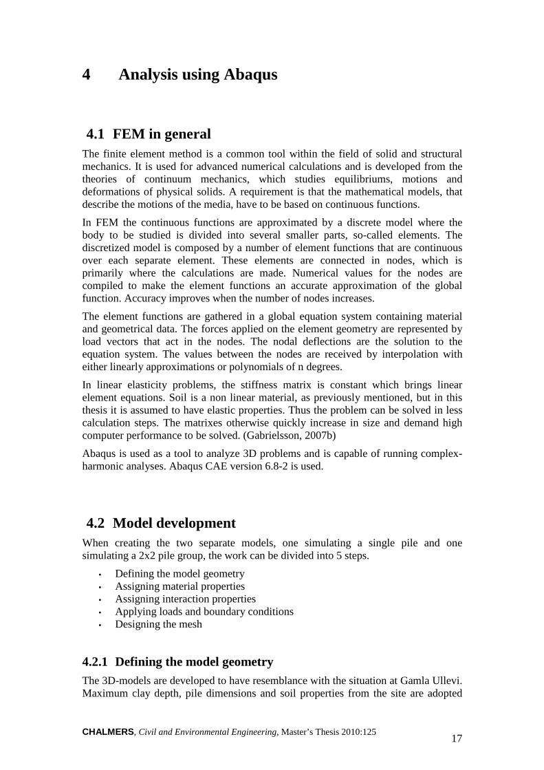
This graph is used for comparison and validation of the response curves obtained from the simulations of the pile head displacements. an increasing displacement up to the natural frequency of the system where the amplitude peaks. At higher frequencies the amplitude decreases and closes to zero.

Figure 3.

Figure 3.9. A normalized 1971)


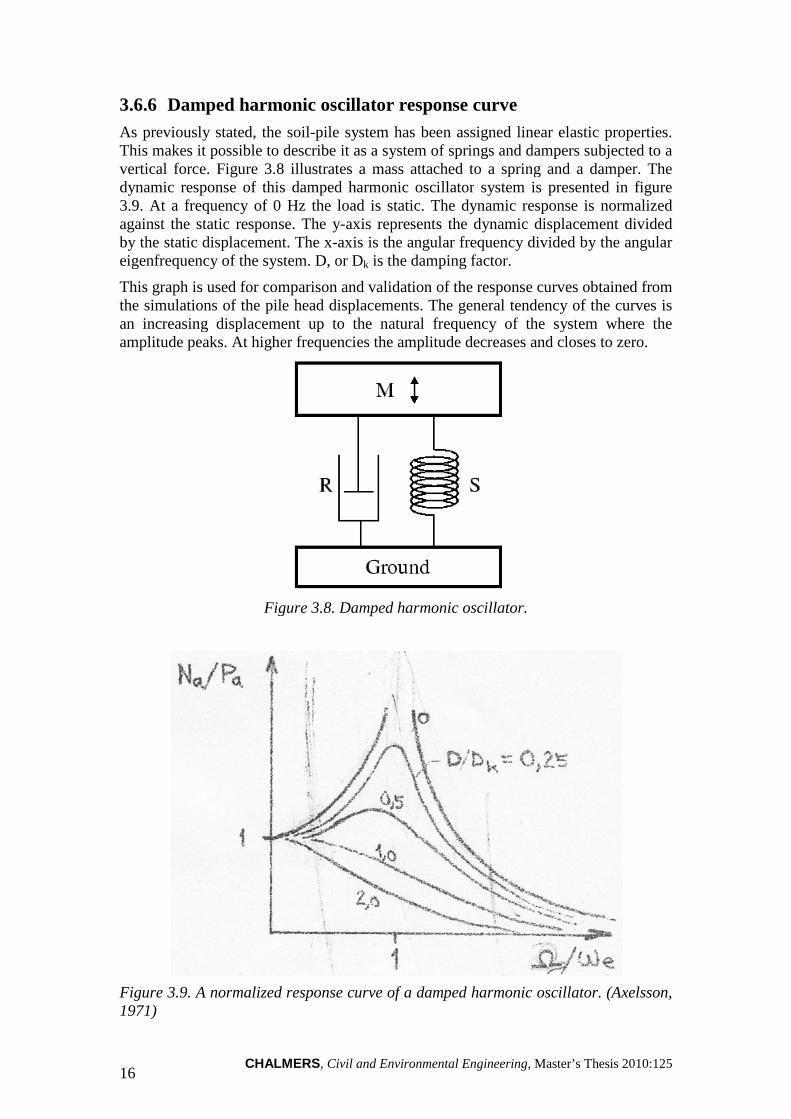
Damped harmonic oscillator response curve As previously stated, the soil-pile system has been assigned linear elastic properties. This makes it possible to describe it as a system of springs and dampers subjected to a

illustrates a mass attached to a spring and a damper.this damped harmonic oscillator system is presented in

At a frequency of 0 Hz the load is static. The dynamic response is normalized against the static response. The y-axis represents the dynamic displacement divided

the static displacement. The x-axis is the angular frequency divided by the angular eigenfrequency of the system. D, or Dk is the damping factor.

This graph is used for comparison and validation of the response curves obtained from pile head displacements. The general tendency

an increasing displacement up to the natural frequency of the system where the amplitude peaks. At higher frequencies the amplitude decreases and closes to zero.

Figure 3.8. Damped harmonic oscillator.

response curve of a damped harmonic oscillator.


pile system has been assigned linear elastic properties. This makes it possible to describe it as a system of springs and dampers subjected to a

a mass attached to a spring and a damper. The system is presented in figure

At a frequency of 0 Hz the load is static. The dynamic response is normalized axis represents the dynamic displacement divided

axis is the angular frequency divided by the angular

This graph is used for comparison and validation of the response curves obtained from of the curves is

an increasing displacement up to the natural frequency of the system where the amplitude peaks. At higher frequencies the amplitude decreases and closes to zero.

curve of a damped harmonic oscillator. (Axelsson,


4 Analysis using Abaqus

4.1 FEM in general The finite element method is a common tool within the field of solid and structural mechanics. It is used for advanced numerical calculations and is developed from the theories of continuum mechanics, which studies equilibriums, motions and deformations of physical solids. A requirement is that the mathematical models, that describe the motions of the media, have to be based on continuous functions.

In FEM the continuous functions are approximated by a discrete model where the body to be studied is divided into several smaller parts, so-called elements. The discretized model is composed by a number of element functions that are continuous over each separate element. These elements are connected in nodes, which is primarily where the calculations are made. Numerical values for the nodes are compiled to make the element functions an accurate approximation of the global function. Accuracy improves when the number of nodes increases.

The element functions are gathered in a global equation system containing material and geometrical data. The forces applied on the element geometry are represented by load vectors that act in the nodes. The nodal deflections are the solution to the equation system. The values between the nodes are received by interpolation with either linearly approximations or polynomials of n degrees.

In linear elasticity problems, the stiffness matrix is constant which brings linear element equations. Soil is a non linear material, as previously mentioned, but in this thesis it is assumed to have elastic properties. Thus the problem can be solved in less calculation steps. The matrixes otherwise quickly increase in size and demand high computer performance to be solved. (Gabrielsson, 2007b)

Abaqus is used as a tool to analyze 3D problems and is capable of running complex-harmonic analyses. Abaqus CAE version 6.8-2 is used.

4.2 Model development When creating the two separate models, one simulating a single pile and one simulating a 2x2 pile group, the work can be divided into 5 steps.

• Defining the model geometry • Assigning material properties • Assigning interaction properties • Applying loads and boundary conditions • Designing the mesh

4.2.1 Defining the model geometry The 3D-models are developed to have resemblance with the situation at Gamla Ullevi. Maximum clay depth, pile dimensions and soil properties from the site are adopted

CHALMERS18

into the models. The elements are 8Geometrical dimensions are presented below.

• Cylindrical soil body: depth 84 m, radius: 100 m.• Pile: length 44m, square cross section of 0.27

Both single pile and pile group are situated in the center of the cylinder.The soil is divided into 8 of 2x2 piles with equal spacing

Figure 4.1. Cylindrical soil body with


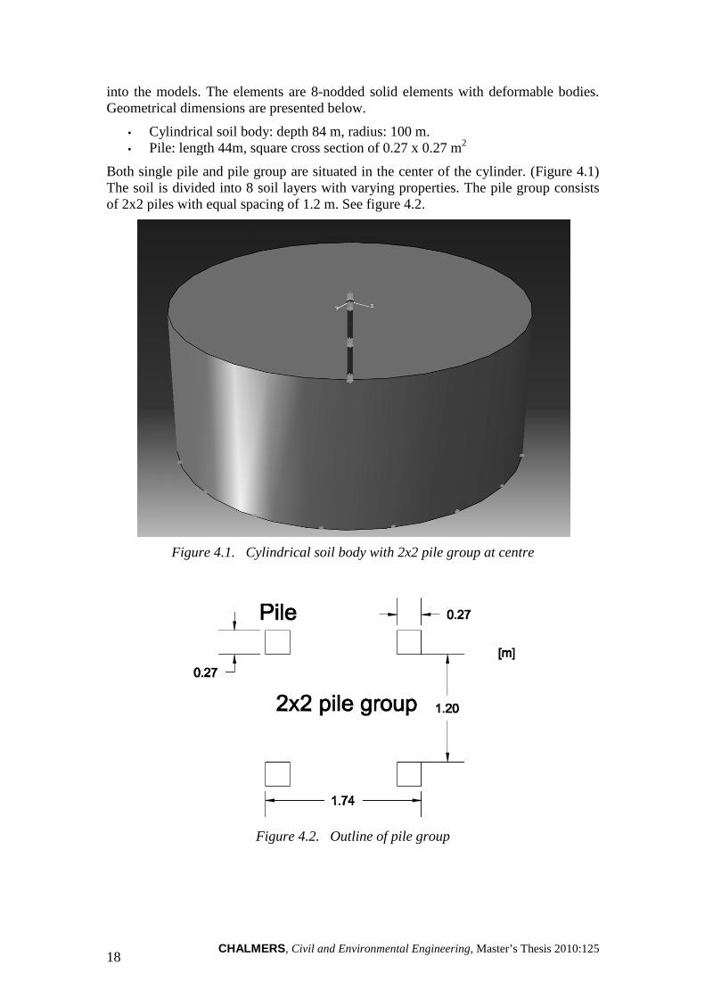
The elements are 8-nodded solid elements with deformable bodies. Geometrical dimensions are presented below.

Cylindrical soil body: depth 84 m, radius: 100 m. ile: length 44m, square cross section of 0.27 x 0.27 m2

Both single pile and pile group are situated in the center of the cylinder. soil layers with varying properties. The pile group consists

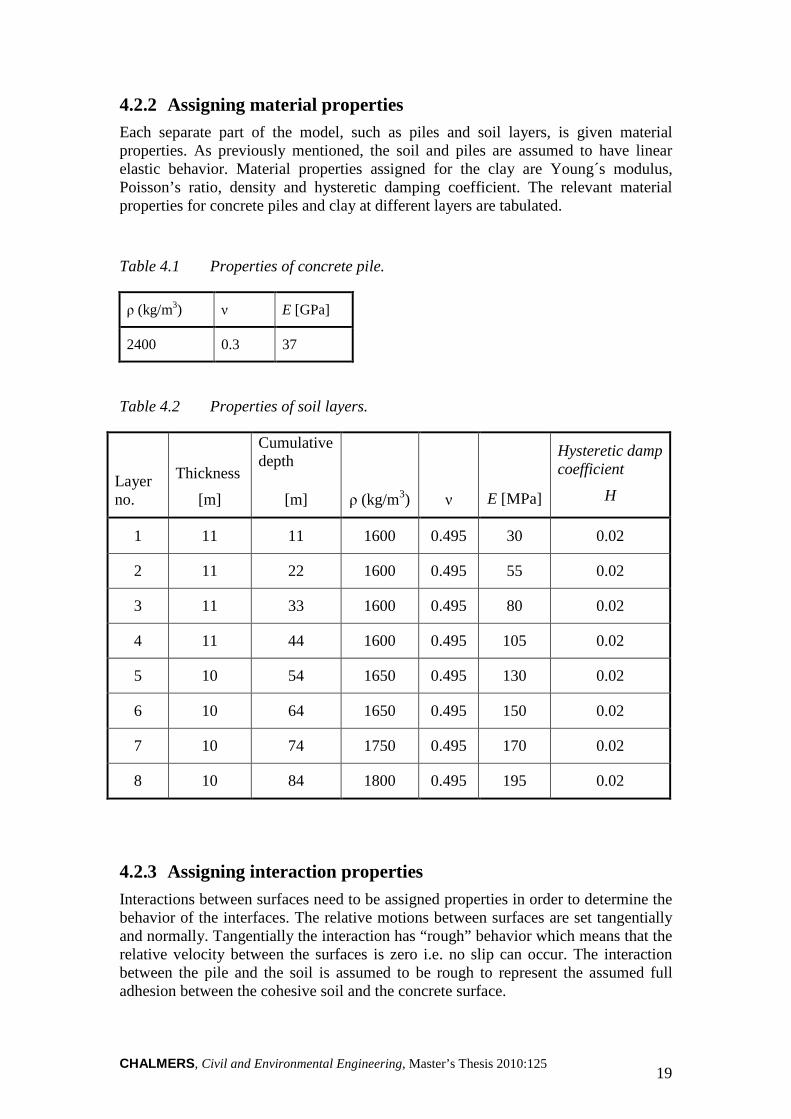
of 2x2 piles with equal spacing of 1.2 m. See figure 4.2.

Figure 4.1. Cylindrical soil body with 2x2 pile group at centre

Figure 4.2. Outline of pile group


nodded solid elements with deformable bodies.

Both single pile and pile group are situated in the center of the cylinder. (Figure 4.1) The pile group consists

at centre


4.2.2 Assigning material properties Each separate part of the model, such as piles and soil layers, is given material properties. As previously mentioned, the soil and piles are assumed to have linear elastic behavior. Material properties assigned for the clay are Young´s modulus, Poisson’s ratio, density and hysteretic damping coefficient. The relevant material properties for concrete piles and clay at different layers are tabulated.

Table 4.1 Properties of concrete pile.

ρ (kg/m3) ν E [GPa]

2400 0.3 37

Table 4.2 Properties of soil layers.

Layer no.

Thickness

[m]

Cumulative depth

[m] ρ (kg/m3)

ν

E [MPa]

Hysteretic damp coefficient

H

1 11 11 1600 0.495 30 0.02

2 11 22 1600 0.495 55 0.02

3 11 33 1600 0.495 80 0.02

4 11 44 1600 0.495 105 0.02

5 10 54 1650 0.495 130 0.02

6 10 64 1650 0.495 150 0.02

7 10 74 1750 0.495 170 0.02

8 10 84 1800 0.495 195 0.02

4.2.3 Assigning interaction properties Interactions between surfaces need to be assigned properties in order to determine the behavior of the interfaces. The relative motions between surfaces are set tangentially and normally. Tangentially the interaction has “rough” behavior which means that the relative velocity between the surfaces is zero i.e. no slip can occur. The interaction between the pile and the soil is assumed to be rough to represent the assumed full adhesion between the cohesive soil and the concrete surface.


Normally the contact is set to “hard” which implies that a contact constrain is applied when the clearance between two surfaces is zero and a positive pressure is established. Separation occurs when the contact pressure between the surfaces is zero or becomes negative. Then the contact constrain is removed.

4.2.4 Applying loads and boundary conditions The jumping audience at Gamla Ullevi subjected the foundation to a dynamic load near 2 Hz. Many of the attendants were not capable of keeping a common jumping rate. Hence the load was not applied as cyclic impulses but according to a harmonic distribution. This is characterized in the FE-model by applying a direct-solution steady-state dynamic analysis where the steady-state harmonic response is calculated using mass, damping and stiffness matrices of the system. In the analysis a frequency range of 0-10 Hz is specified together with a linear frequency spacing. This is to find possible trends or resonance effects in a wider frequency range. The magnitude of the dynamic load is set, as previously mentioned, to 5 kN.

The nodes at the lower boundary surface of the soil are fixed (zero displacement and rotation) in order to model the bedrock. This generates reflecting waves which has to be considered when the results from the simulations are being analyzed. If waves are allowed to reflect the system can maintain standing waves and then has one or several eigenfrequencies.

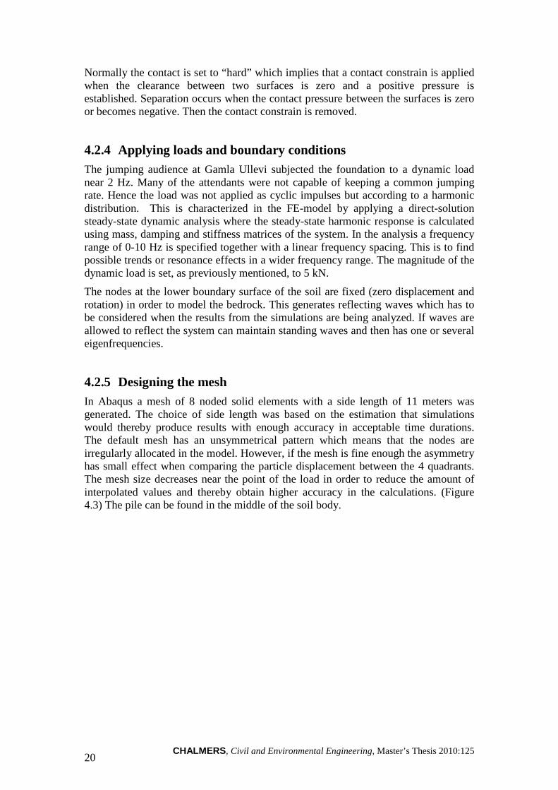
4.2.5 Designing the mesh In Abaqus a mesh of 8 noded solid elements with a side length of 11 meters was generated. The choice of side length was based on the estimation that simulations would thereby produce results with enough accuracy in acceptable time durations. The default mesh has an unsymmetrical pattern which means that the nodes are irregularly allocated in the model. However, if the mesh is fine enough the asymmetry has small effect when comparing the particle displacement between the 4 quadrants. The mesh size decreases near the point of the load in order to reduce the amount of interpolated values and thereby obtain higher accuracy in the calculations. (Figure 4.3) The pile can be found in the middle of the soil body.


Figure 4.3. Generated mesh, single pile

4.3 FEM output Below is a presentation of response curves obtained from the simulated loading cases. The y-axis represents the vertical displacement in frequency range of 0-10 Hz.

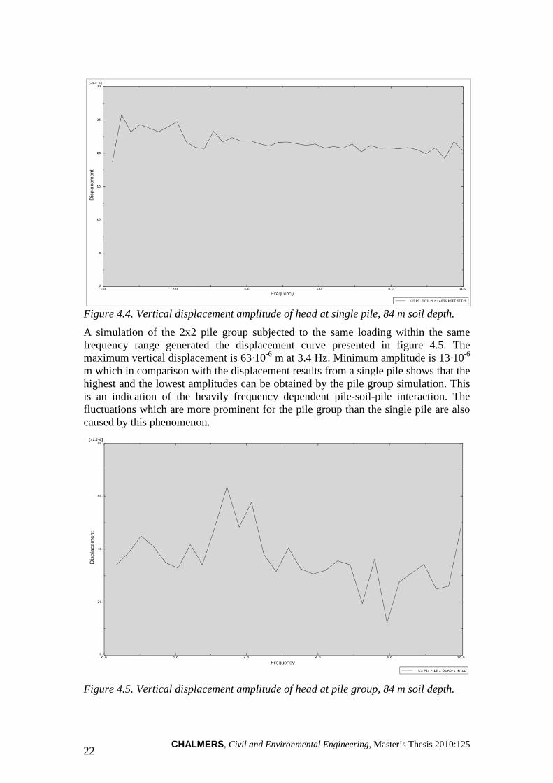
Simulation of a dynamic load on a below in figure 4.4. The frequency range is 0displacement is 25·10-6 m which cawhere the curve exhibits highest fluctuations. The general tendencydisplacement amplitude towards higher frequencies. frequency can be considered as uniform

In comparison with the damped oscillation curve in figure 3.10 no eigenfreqbe found in figure 4.4 within expected to occur from vertical the bedrock.


Figure 4.3. Generated mesh, single pile

Below is a presentation of response curves obtained from the simulated loading cases.

axis represents the vertical displacement in 10-6 m. The x-axis represents the 10 Hz.

dynamic load on a single pile resulted in the displacement curve seen The frequency range is 0-10 Hz and the maximum vertical

m which can be found in the range 0.5-2.1 Hz.where the curve exhibits highest fluctuations. The general tendency

amplitude towards higher frequencies. The amplitudes for each specific frequency can be considered as uniform with values between 20·10-6 m

In comparison with the damped oscillation curve in figure 3.10 no eigenfreqwithin the generated frequency range. The resonance effect is vertical P-waves generated from the pile and reflect

21

Below is a presentation of response curves obtained from the simulated loading cases. axis represents the

single pile resulted in the displacement curve seen the maximum vertical

Hz. This is also where the curve exhibits highest fluctuations. The general tendency is decreasing

s for each specific m to 25·10-6 m.

In comparison with the damped oscillation curve in figure 3.10 no eigenfrequency can The resonance effect is

reflected against

CHALMERS22

Figure 4.4. Vertical displacement amplitude of

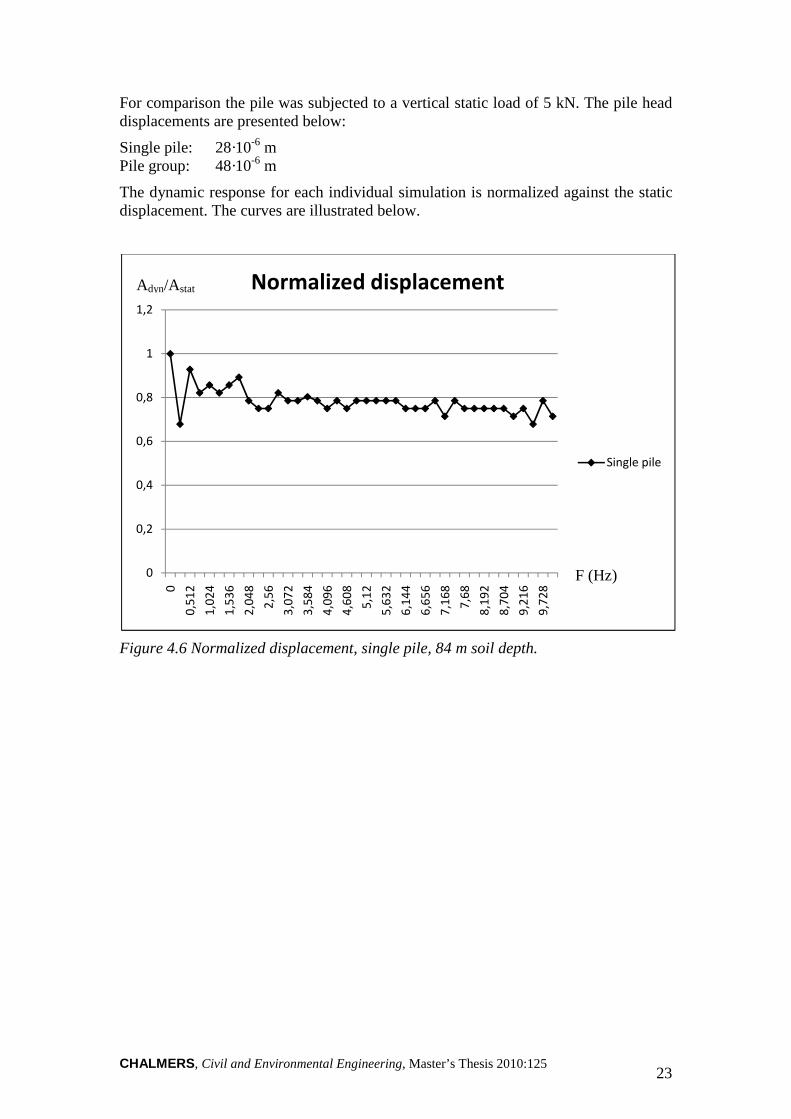
A simulation of the 2x2 frequency range generated maximum vertical displacement is 6m which in comparison with the displacement results from a single pile shows that the highest and the lowest amplitudes can be obtained by the pile group simulation. This is an indication of the heavily frequency dependefluctuations which are more prominent for the caused by this phenomenon.

Figure 4.5. Vertical displacement amplitude of head at pile group


cal displacement amplitude of head at single pile, 84 m soil depth

pile group subjected to the same loading within the same frequency range generated the displacement curve presented in figure 4.5.maximum vertical displacement is 63·10-6 m at 3.4 Hz. Minimum amplitude is 1m which in comparison with the displacement results from a single pile shows that the highest and the lowest amplitudes can be obtained by the pile group simulation. This

heavily frequency dependent pile-soil-pile interaction.fluctuations which are more prominent for the pile group than the single pile are also caused by this phenomenon.

Figure 4.5. Vertical displacement amplitude of head at pile group, 84 m soil depth


, 84 m soil depth.

within the same the displacement curve presented in figure 4.5. The

Minimum amplitude is 13·10-6 m which in comparison with the displacement results from a single pile shows that the highest and the lowest amplitudes can be obtained by the pile group simulation. This

pile interaction. The pile group than the single pile are also

, 84 m soil depth.


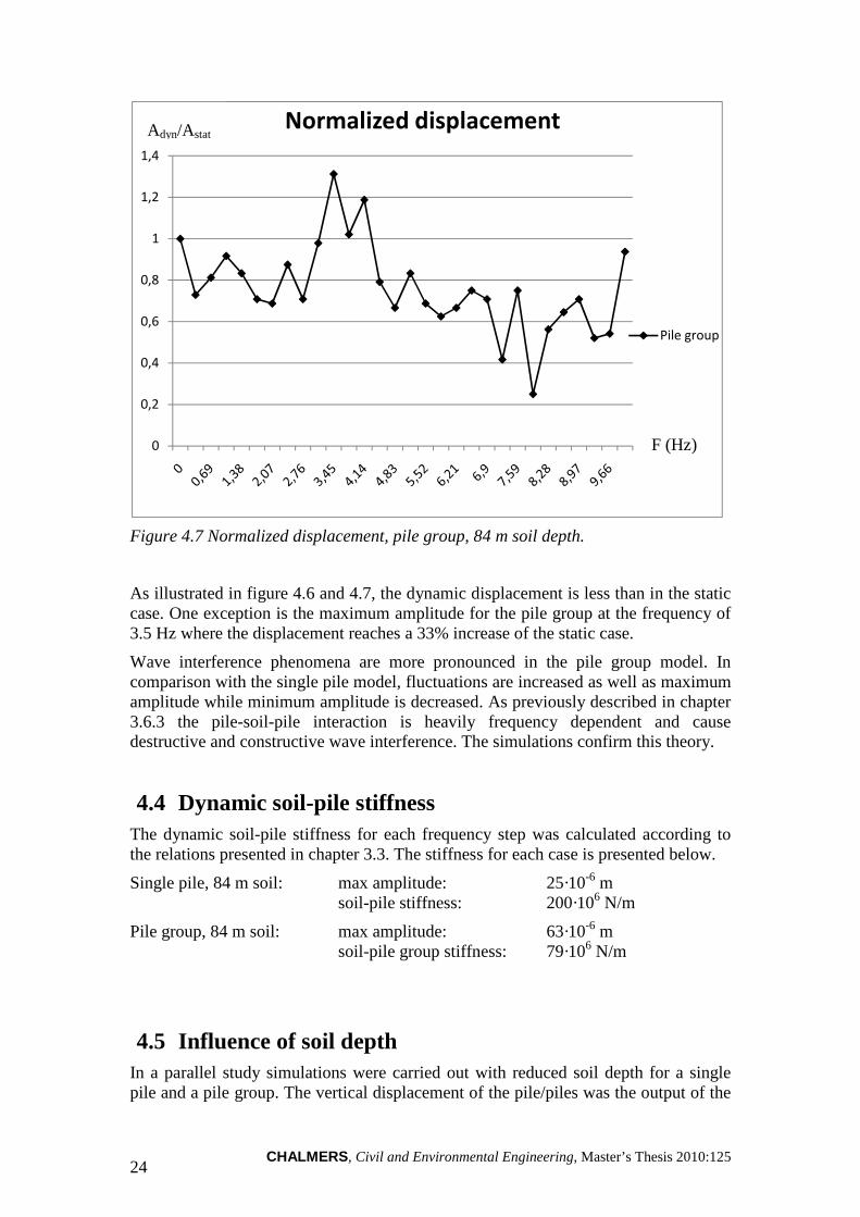
For comparison the pile was subjected to a vertical static load of 5 kN. The pile head displacements are presented below:

Single pile: 28·10-6 m Pile group: 48·10-6 m

The dynamic response for each individual simulation is normalized against the static displacement. The curves are illustrated below.

Figure 4.6 Normalized displacement, single pile, 84 m soil depth.

0

0,2

0,4

0,6

0,8

1

1,2

0

0,5

12

1,0

24

1,5

36

2,0

48

2,5

6

3,0

72

3,5

84

4,0

96

4,6

08

5,1

2

5,6

32

6,1

44

6,6

56

7,1

68

7,6

8

8,1

92

8,7

04

9,2

16

9,7

28

Normalized displacement

Single pile

Adyn/Astat

F (Hz)


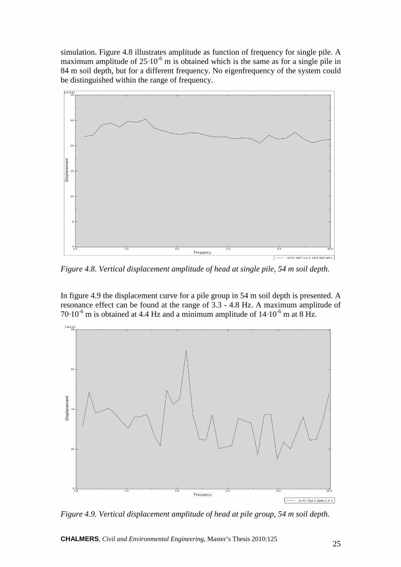
Figure 4.7 Normalized displacement, pile group, 84 m soil depth.

As illustrated in figure 4.6 and 4.7, the dynamic displacement is less than in the static case. One exception is the maximum amplitude for the pile group at the frequency of 3.5 Hz where the displacement reaches a 33% increase of the static case.

Wave interference phenomena are more pronounced in the pile group model. In comparison with the single pile model, fluctuations are increased as well as maximum amplitude while minimum amplitude is decreased. As previously described in chapter 3.6.3 the pile-soil-pile interaction is heavily frequency dependent and cause destructive and constructive wave interference. The simulations confirm this theory.

4.4 Dynamic soil-pile stiffness The dynamic soil-pile stiffness for each frequency step was calculated according to the relations presented in chapter 3.3. The stiffness for each case is presented below.

Single pile, 84 m soil: max amplitude: 25·10-6 m soil-pile stiffness: 200·106 N/m

Pile group, 84 m soil: max amplitude: 63·10-6 m soil-pile group stiffness: 79·106 N/m

4.5 Influence of soil depth In a parallel study simulations were carried out with reduced soil depth for a single pile and a pile group. The vertical displacement of the pile/piles was the output of the

0

0,2

0,4

0,6

0,8

1

1,2

1,4

Normalized displacement

Pile group

Adyn/Astat

F (Hz)


simulation. Figure 4.8 illustrates amplitude as function of frequency formaximum amplitude of 25·1084 m soil depth, but for a different frequency. be distinguished within the

Figure 4.8. Vertical displacement amplitude of head at single pile

In figure 4.9 the displacement curve for a pile group resonance effect can be found70·10-6 m is obtained at 4.4 Hz and a minimum amplitude of 14

Figure 4.9. Vertical displacement am


Figure 4.8 illustrates amplitude as function of frequency formaximum amplitude of 25·10-6 m is obtained which is the same as for a s84 m soil depth, but for a different frequency. No eigenfrequency of the system could

the range of frequency.

Vertical displacement amplitude of head at single pile, 54 m soil depth

In figure 4.9 the displacement curve for a pile group in 54 m soil depth resonance effect can be found at the range of 3.3 - 4.8 Hz. A maximum amplitude of

is obtained at 4.4 Hz and a minimum amplitude of 14·10-6 m

Figure 4.9. Vertical displacement amplitude of head at pile group, 54 m soil depth.

25

Figure 4.8 illustrates amplitude as function of frequency for single pile. A m is obtained which is the same as for a single pile in

No eigenfrequency of the system could

, 54 m soil depth.

in 54 m soil depth is presented. A A maximum amplitude of

at 8 Hz.

4 m soil depth.


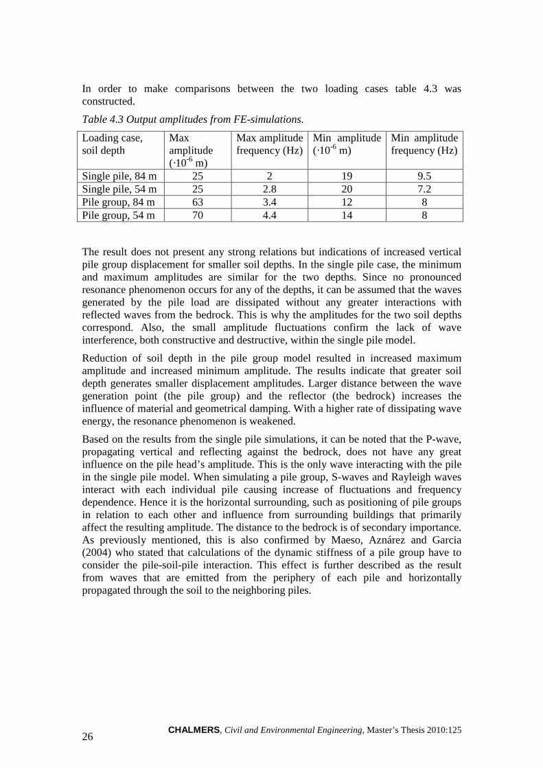
In order to make comparisons between the two loading cases table 4.3 was constructed.

Table 4.3 Output amplitudes from FE-simulations.

Loading case, soil depth

Max amplitude (·10-6 m)

Max amplitude frequency (Hz)

Min amplitude (·10-6 m)

Min amplitude frequency (Hz)

Single pile, 84 m 25 2 19 9.5 Single pile, 54 m 25 2.8 20 7.2 Pile group, 84 m 63 3.4 12 8 Pile group, 54 m 70 4.4 14 8

The result does not present any strong relations but indications of increased vertical pile group displacement for smaller soil depths. In the single pile case, the minimum and maximum amplitudes are similar for the two depths. Since no pronounced resonance phenomenon occurs for any of the depths, it can be assumed that the waves generated by the pile load are dissipated without any greater interactions with reflected waves from the bedrock. This is why the amplitudes for the two soil depths correspond. Also, the small amplitude fluctuations confirm the lack of wave interference, both constructive and destructive, within the single pile model.

Reduction of soil depth in the pile group model resulted in increased maximum amplitude and increased minimum amplitude. The results indicate that greater soil depth generates smaller displacement amplitudes. Larger distance between the wave generation point (the pile group) and the reflector (the bedrock) increases the influence of material and geometrical damping. With a higher rate of dissipating wave energy, the resonance phenomenon is weakened.

Based on the results from the single pile simulations, it can be noted that the P-wave, propagating vertical and reflecting against the bedrock, does not have any great influence on the pile head’s amplitude. This is the only wave interacting with the pile in the single pile model. When simulating a pile group, S-waves and Rayleigh waves interact with each individual pile causing increase of fluctuations and frequency dependence. Hence it is the horizontal surrounding, such as positioning of pile groups in relation to each other and influence from surrounding buildings that primarily affect the resulting amplitude. The distance to the bedrock is of secondary importance. As previously mentioned, this is also confirmed by Maeso, Aznárez and Garcia (2004) who stated that calculations of the dynamic stiffness of a pile group have to consider the pile-soil-pile interaction. This effect is further described as the result from waves that are emitted from the periphery of each pile and horizontally propagated through the soil to the neighboring piles.


5 Discussion on results from the analysis In the Gamla Ullevi case FEM was used as a tool to investigate the vibration amplitudes at the football stadium caused by the jumping audience. This helped in evaluating the expected reduction effect by a number of different measures. The model represented an idealized and simplified loading case e.g. by excluding lateral loads. Time constraints for the project prevented the development of a complete model of the site. Hence, the simulation results should be primarily considered as indicators of expected vibrations. For this particular loading case it was a valuable tool since no analytical solution could be found during the literature study for this thesis. Since there is a lack of previously verified solutions the FE models were evaluated by comparing the results to a normalized response curve of a damped harmonic oscillator. The FE program chosen for this thesis was Abaqus and in order to further verify the results additional models could be developed in other FE programs e.g. Plaxis 3D.

This thesis is intended to function as a guideline for geotechnicians when modeling foundations in soils sensitive to dynamic loading. The results compiled from the analysis bring increased knowledge of dynamic loading cases in soil and the pile-soil-pile interaction experienced in the pile group case. The output from the FE program is specific for this case but is used to verify and to point out the importance of considering the pile-soil-pile interaction when vibrations in structures are studied. Other wave generating activities can be found such as train and tram movements which make vibrations a common phenomenon in the Gothenburg area.

The FE models were developed and run in the 3D simulation program Abaqus. The average time duration for one simulation of 50 calculation points was 20 minutes. Abaqus capability of running models in three dimensions makes it possible to simulate complex and realistic loading cases. FE programs can therefore function as an effective tool for engineers involved in construction projects. If the models are developed by experienced staff the time requirement for compilation of these results should be acceptable.

In the case of Gamla Ullevi, the analysis showed the complex nature of dynamic loading. The frequency corresponding to the maximum deflection amplitude is heavily dependent on the surrounding area which requires extensive work in FE modeling. Thus it is difficult to predict the eigenfrequency of a system of this size. The accuracy of the results is dependent on the chosen element size. The element size used in this study was adjusted to measure up to the capacity of the computers. Also the number of calculation points within the chosen frequency range affects the quality of the result.

More studies need to be carried out in this subject and a number of suggestions to help improve the knowledge in this topic are presented next.


5.1 Suggestions of further studies As a first step a number of assumptions were made to reduce the amount of parameters in the analysis. This made the FE model manageable and easier to get an overview of. However, it is undetermined to what extent these parameters affect the dynamic stiffness.

Isotropy

The analysis included assumptions that the soil and the piles had isotropic properties. It would be of interest to compare the results with a similar analysis that includes the anisotropic behavior of soil and the orthotropic properties of the piles.

Nonlinearity

In this thesis, the analysis is limited to linear dynamics by assuming the load to be small enough not to induce nonlinear behaviors. Nevertheless, nonlinear behaviors can be induced if the load is large enough. The contingency of when a nonlinear analysis is required increases the uncertainty of the simulated output. It would be of interest to investigate what magnitudes of loading that require the nonlinear analysis.

Permeability

In order to increase the accuracy of the simulated results additional soil parameters should be included in the analysis. As mentioned in chapter 3.6.3 the soil-pile stiffness is influenced by the soil permeability. High permeability produces lower values of soil-pile stiffness. This is an example of one relation that is not yet incorporated within the Abaqus software.

Lateral loads

Practically, a pile is subjected to lateral actions even though the predominant type of loading is an axial force. To get a complete view of the Gamla Ullevi case lateral loads should be included. There are occasions when lateral loads can be considerable e.g. on coastal structures where water waves and wind loads are prominent. In such cases the dynamic lateral stiffness becomes a factor to consider in the pile design.

Pile-soil-pile interaction In this analysis the pile-soil-pile interaction was studied between piles within the same pile group. Further studies of this interaction should include interaction between two or more pile groups. It is an interesting topic to analyze how the number of piles, the dimensioning of piles and the distance between the pile groups affect the deflection amplitude of the foundation.


6 Conclusions

In a simulated comparison between a 2x2 pile group and a single pile subjected to a dynamic load the pile group was found to exhibit lowest soil-pile stiffness at a specific frequency. Within a frequency interval of 0-10 Hz the pile group also displayed the highest soil-pile stiffness and greater fluctuations which makes the stiffness heavily frequency dependent. This is due to the pile-soil-pile interaction that occurs within the pile group.

Simulations showed that the vertical distance between the piles and the bedrock has little influence on the displacement amplitude of the pile head. The maximum amplitude for a single pile was unchanged and the corresponding frequency varied 0.8 Hz. Instead variations of the horizontal surrounding were found to have greater impact on the displacement amplitude. It also affected the frequency at which resonance occurred.

Accuracy of the output from the simulations can be improved through further investigations. This includes further development of the model by implementing additional material parameters e.g. soil permeability and assign anisotropic properties to the soil and orthotropic properties to the piles. The outcome of the result is also dependent on the chosen element size and the number of increments chosen within the frequency interval.

The analysis included simulations using the FE software Abaqus in which a number of 3D models were developed. One simulation of 50 calculation points in a frequency interval of 0-10 Hz had an average time duration of 20 minutes. FE programs were found to be a useful tool in investigations concerning dynamic loads on structure foundations.


References

Axelsson K. (1971) Introduktion till byggnadsdynamiken. Chalmers tekniska högskola, Göteborg. pp 8

Brinkgreve, Broere & Waterman. (2006) Plaxis 2D Dynamics manual version 9.0. Delft, Netherlands.

Engineering Fundamentals (2010) http://www.efunda.com (2010-06-08)

Ewins D.J. (1984) Modal Testing: Theory and Practice. Brüel & Kjaer, Letchworth, England. pp. 26-27.

Gabrielsson J. (2007a) Numerisk simulering av stabilitet för vägbank på sulfidjord – jämföerelser med fältmätning. Luleå tekniska universitet, Sverige. pp. 18-19.

Gabrielsson J. (2007b) Numerisk simulering av stabilitet för vägbank på sulfidjord – jämföerelser med fältmätning. Luleå tekniska universitet, Sverige. pp. 8-10.

Gatubolaget. (2006) Rapport över geotekniska och markmiljöundersökningar för Fotbollsarenan, Heden 705:14 m fl. Göteborg, Sweden

Helwany S. (2007) Applied soil mechanics with abaqus applications. John Wiley & Sons,Inc., Hoboken, New jersey.pp. 23

Hügel, Henke, Kinzler. (2008) High-performance Abaqus simulations in soil mechanics. Hamburg University of Technology, Germany. pp. 4

Kungliga Ingenjörsvetenskapsakademin (IVA) (1979) Jord- och bergdynamik. Meddelande 225. Stockholm, Sverige.

Kramer S.L. (1996) Geotechnical earthquake engineering. 3ed. Prentice Hall, Inc., Upper Saddle River, New Jersey.

Maheshwari, B.K. & Watanabe, H. (2005) Dynamic analysis of pile foundations. Saitama University, Japan. Paper


Maheshwari, B.K. & Watanabe, H. (1997) Nonlinear dynamic analysis of pile foundation. Japan, Saitama University. Paper

Norconsult AB. (2009) Göteborg/HIGAB Gamla Ullevi, Vibrationer – PM beträffande vibrationskontroll. pp 8-10.

Skredkommisionen (1995) Anvisningar för släntstabilitetsutredning. Rapport 3:95. Linköping, Sverige. pp. 5.26

Maeso O., Aznárez J., García F. (2004a) Dynamic impedances of piles and groups of piles in saturated soils. Computers and Structures, No. 83, January 2005, pp. 773.

Maeso O., Aznárez J., García F. (2004b) Dynamic impedances of piles and groups of piles in saturated soils. Computers and Structures, No. 83, January 2005, pp. 775, 780.

Maeso O., Aznárez J., García F. (2004c) Dynamic impedances of piles and groups of piles in saturated soils. Computers and Structures, No. 83, January 2005, pp. 776-777.

Möller B., Larsson R., Bengtsson P-E., Moritz L. (2000) Geodynamik i praktiken. Information 17. Statens geotekniska institute (SGI) Linköping, Sverige. pp. 10-15

Parrales R. (2004) Different definitions of energy dissipation in geological materials. Lund Institute of Technology, Sweden.

Seed H. B., Idriss I. M. (1970) Soil Moduli and Damping Factors for Dynamic Response Analyzes. Report No. EERC 70-10, University of California, Berkeley.

Simulia (2010) Abaqus version 6.8 documentation. USA.

Telford, Geldart, Sheriff, Keys (1978) Applied Geophysics. New York, U.S.A. Cambridge University Press. pp. 251.


Appendices

Appendix A - Site plan of Gamla Ullevi

Appendix B – Measurements from site investigation, Gatubolaget 2006


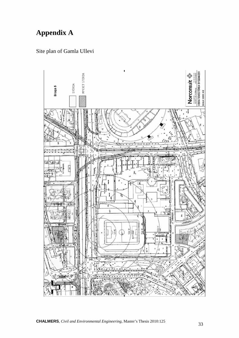
Appendix A

Site plan of Gamla Ullevi


Site plan of Gamla Ullevi

33

CHALMERS34

Appendix B

Measurements from s

Undrained shear strength


Measurements from site investigations, Gatubolaget 2006

Undrained shear strength


Gatubolaget 2006


Density

Civil and Environmental Engineering, Master’s Thesis 2010:125 35

CHALMERS36

Preconsolidation pressure


Preconsolidation pressure


Documents

Analysis of the dynamic stiffness of a soil-pile system ...Analysis of the dynamic stiffness of a soil-pile system using Abaqus Master of Science Thesis in the Master’s Programme